chapter 16: the analysis of variance...

Chapter 16: The Analysis of Variance (ANOVA)

This handout is downloadable at www.migomendoza.weebly.com

Chapter 16: The Analysis of Variance

(ANOVA)

Recall:

In the last two chapters we dealt with situations in which we have one independent variable with two levels. In many instances, however, we may have an independent variable with three or more levels. Pre-Example 1:

Suppose we are interested in determining if there is a significant difference in the per capita income between residents of Canada, the United States, and Mexico. Question:

From there, what will be our research and null hypothesis?

Research Hypothesis: "There will be a significant difference in the average per capita income between citizens of Canada,

the United States, and Mexico." Null Hypothesis: "There will be no significant difference in the average per capita income between citizens of Canada,

the United States, and Mexico." Question:

What will be our independent variable? How many levels and what are they? What is our dependent variable?

Answer: Our independent variable is "Country" and the three different countries represent three

levels. The dependent variable is the average income for each country's citizens. Note:

In our dependent variable, income for each country's citizens can be measured using quantitative type of data. That is, ratio.

Question: Given all of this, which statistical test can we use?

Danger Here: A lot of beginning statisticians say using three separate independent-sample t-tests would

fit. They are right. Those three comparisons are inclusive of all of the comparisons that could be made between the three countries, but using three different t-tests creates a problem.

Keeping that in mind, think what might happen if we used three independent-sample t-tests to test our hypothesis. In essence, we would be using an alpha value of .05 three different times in order to test one overall hypothesis. Obviously, this is going to greatly inflate our possibility of making a Type I error.

http://www.migomendoza.weebly.com/



Lesson 16.1: The Brief History of ANOVA and Ronald Fisher

Ronald Fisher

He is an agronomist who developed the analysis of variance or, as it is most always abbreviated, ANOVA. The Brief History of ANOVA

Fisher is originally an astronomer who began working in 1919 as a biologist for an agricultural station in England. He greatly contributed to the fields of genetics and statistics. His list of accomplishments in statistics and genetics is so great and his awards are so impressive that he was even knighted by Queen Elizabeth in 1952.

Fisher felt that the only way to accurately investigate significant differences between groups was to look at the variance of scores within each of the levels of the independent variable as well as the variance between the different groups. Understanding the ANOVA Pre-Example 2:

"There will be a significant difference in achievement between students studying math in a

lecture-based classroom, students studying math in a technology-based classroom, and students

studying math in a classroom where both lecture and technology are used." Question:

What is our independent variable? How many levels and what are they? What is our dependent variable? Can we collect a quantitative data from our dependent variable? Answer:

The independent variable is "instructional type" and there are three levels-"lecture, technology, and a combination of both." The dependent variable is achievement. Yes, we can collect quantitative data, that is, ratio. Hint:

In problems involving three or more levels of independent variable, it is advisable to state a nondirectional hypothesis since it would be difficult to state one null hypothesis that would cover all of the different combinations we could possibly check.

Lesson 16.2: The Different Types of ANOVAs

(1) One-Way ANOVA (2) Factorial ANOVA (3) Multivariate ANOVA

There are several types of ANOVA. The selection of type of ANOVA to use is based on the

number of independent variables, the number of dependent variables, and the type of data collected. NOTE:

If your dependent variables represent nonparametric data, you will be using one of the nonparametric ANOVAs. Suffice it to say that nonparametric ANOVAs exist.




Type 1: One-Way ANOVA

It is the most elementary ANOVA. When we say something is "one way," we mean there is only one independent variable and one dependent variable. The independent variable can have three or more levels, and the dependent variable represents quantitative data. Type 2: Factorial ANOVA

When we say an ANOVA is "factorial," we simply mean there is more than one independent variable and only one dependent variable. One of the most common ways we refer to factorial ANOVA is by stating the number of independent variables.

(1) Three-Way ANOVA If we have a three-way ANOVA, we are saying we have a factorial ANOVA with three

independent variables. (2) Two-Way ANOVA

If we have a two-way ANOVA, we are saying we have a factorial ANOVA with two independent variables.

(3) Four-Way ANOVA If we have a four-way ANOVA, we are saying we have a factorial ANOVA with four

independent variables. NOTE:

Sometimes we take it a step further and tell the reader the number of levels within each of the independent variables. Pre-Example 3:

Let's say we had a two-way ANOVA where the independent variables were "college class" and "gender" and we are interested in using it to determine if there is a significant difference in achievement. Question:

How many levels do we have in "college class" independent variable? How about "gender" independent variable? Do you know?

In order to be as clear as possible, someone performing research using this particular ANOVA might call it a "4 X 2 (four by two) ANOVA” rather than just a factorial ANOVA. NOTE:

The great thing about using this annotation is we can tell exactly how many measurements we are going to make by multiplying the two numbers together. Thus, here we would be collecting eight measurements (𝟒 𝒙 𝟐 = 𝟖).

Table 16.1 Cells for Gender and Class for Factorial ANOVA




Pre-Example 4: We might have a three-way ANOVA where we are collecting data about:

(1) the gender of a child; (2) whether or not the child went to kindergarten; and (3) the number of parents in the home.

Task:

Based on this information, construct a null hypothesis. Null Hypothesis: "There is no significant difference in achievement of first graders in their gender, whether or not

they went to kindergarten, and the number of parents in their home." Question:

Based on the information given, what kind of factorial ANOVA can we have? Answer:

Here, we would have a three-way ANOVA because we have three independent variables. Question:

How many levels do we have in "gender" independent variable? "kindergarten attendance" independent variable? "number of parents" variable? Use this information to provide an annotation for our factorial ANOVA. Answer:

This three-way ANOVA could also be called a 2 X 2 X 2 ANOVA because gender has two levels, male or female; kindergarten attendance has two levels, yes or no; and number of parents in the home has two levels, in this case one or two parents.

Table 16.2 Cells for Gender and Number of Parents for Factorial ANOVA

Type 3: Multivariate ANOVA

This is a type of ANOVA where we have more than one dependent variable, regardless of the number of independent variables. It is also called as MANOVA (multivariate analysis of variance). Pre-Example 5:

Suppose we have three groups of students and we want to measure their intrinsic motivation and achievement.




Question: How many independent variables do we have? How many levels? How many dependent

variables? Answer:

In this case, we have one independent variable (i.e., group of students) with three levels and two dependent variables (i.e., gender and intrinsic motivation). Do you know?

The multivariate analysis of variance, because of all the interactions that multiple independent and dependent variables create, can be a complicated test to compute, analyze, and interpret.

Lesson 16.3: Assumptions to Make When Using Any ANOVA

(1) Random Samples (2) Independence of Scores (3) Normal Distribution of Data (4) Homogeneity of Variance

Do you know?

Unfortunately, even when we have the right number of independent and dependent variables and we are collecting the right type of data, sometimes the ANOVA is not the appropriate test to work with. The ANOVA, in fact, works under four major assumptions. Assumption 1: Random Samples

If our dependent variable scores represent a sample of a larger population, then it should be a random sample. Other typed of samples, especially where the researcher picks subjects because of ease or availability, can make the results of the ANOVA not generalizable to other samples or situations. Assumption 2: Independence of Scores

The scores collected are independent of one another. For example, if you are collecting data from school children, this means the score that one child gets is not influenced by, or dependent on, the score received by another child. Assumption 3: Normal Distribution

Each sample or population studied needs to be somewhat normally distributed. As we saw in t-test, this does not mean a perfect bell-shaped distribution is required, but there has to be a certain degree of "normality" for the underlying calculations to work correctly. Assumption 4: Homogeneity of Variance

The "homogeneity of variance" is required. This means that the degree of variance within each of the samples should be about the same. Question:

How will you control assumptions 1 an 2? How will you control assumptions 3? How will you control assumption 4?




Lesson 16.4: Calculating the ANOVA

The computations for the ANOVA are very straightforward. Fisher demonstrated that, in

order to test hypothesis using a one-way analysis of variance, one needed to understand four things:

(1) Total Variance (2) Total Degrees of Freedom (3) Mean Square (4) F Value

Total Variance

The total variance in the data is the sum of the (a) within-group variance and the (b) between-groups variance. Total Degrees of Freedom

This is the sum of the within-group degrees of freedom and the between-groups degrees of freedom. Mean Square

The mean square values for the within-group and between-groups variance. The F Value

The F value that can be calculated using the data from the first three steps. Example 16.1

Suppose we are interested in looking at the effect of different types of medication on headache relief. Here we have three levels: "Pill 1, Pill 2, and Pill 3." The dependent variable, which we will call "time to relief," shows the number of minutes that elapse between the time the pill is taken and the time the headache symptoms are relieved.

Table 16.3 Amount of Time for Pill Type

Calculating the Total Variance

The total variance includes three values:

(1) Total Sum of Squares; (2) The Between Sum of Squares; and (3) The Within Sum of Squares.




Table 16.4 The Computation of Sums of Squares

𝑥1 𝑥12 𝑥2 𝑥2

2 𝑥3 𝑥32

8 6 8

8 6 9

7 5 2

3 4 8

5 2 2

∑ 𝑥1 = ∑ 𝑥12 = ∑ 𝑥2 = ∑ 𝑥2

2 = ∑ 𝑥3 = ∑ 𝑥32 =

The Total Sum of Squares

The total sum of squares is abbreviated as 𝑆𝑆𝑡𝑜𝑡𝑎𝑙 and can be calculated using this formula:

where:

∑ 𝑥2 is the sum of squares of all of individual scores in the dataset. ∑ 𝑥 is the square of sum of all of individual scores in the dataset.

𝑁 is the number of the population. Task 1:

Compute the Total Sum of Squares.

𝑺𝑺𝒕𝒐𝒕𝒂𝒍 85.73

The Between Sum of Squares

The between sum of squares also has a rather lengthy formula:

where: ∑ 𝑥1 is the sum of individual scores in the first group.

∑ 𝑥2 is the sum of individual scores in the second group. ∑ 𝑥3 is the sum of individual scores in the third group.

∑ 𝑥 is the sum of individual scores from first group to third group. 𝑛1 is the number of samples in the first group.

𝑛2 is the number of samples in the second group. 𝑛3 is the number of samples in the third group.

𝑁 is the number of population in the dataset. Task 2:

Compute for the Between Sum of Squares.




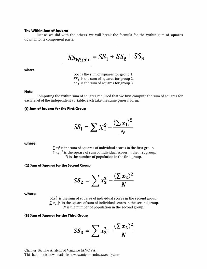
The Within Sum of Squares

Just as we did with the others, we will break the formula for the within sum of squares down into its component parts.

where:

𝑆𝑆1 is the sum of squares for group 1. 𝑆𝑆2 is the sum of squares for group 2. 𝑆𝑆3 is the sum of squares for group 3.

Note:

Computing the within sum of squares required that we first compute the sum of squares for each level of the independent variable; each take the same general form: (1) Sum of Squares for the First Group

where:

∑ 𝑥12 is the sum of squares of individual scores in the first group.

[∑ 𝑥1 ]2 is the square of sum of individual scores in the first group. 𝑁 is the number of population in the first group.

(2) Sum of Squares for the Second Group

𝑺𝑺𝟐 = ∑ 𝒙𝟐𝟐 −

(∑ 𝒙𝟐)𝟐

𝑵

where:

∑ 𝑥22 is the sum of squares of individual scores in the second group.

[∑ 𝑥2 ]2 is the square of sum of individual scores in the second group. 𝑁 is the number of population in the second group.

(3) Sum of Squares for the Third Group

𝑺𝑺𝟑 = ∑ 𝒙𝟑𝟐 −

(∑ 𝒙𝟑)𝟐

𝑵




where:

∑ 𝑥32 is the sum of squares of individual scores in the third group.

[∑ 𝑥3 ]2 is the square of sum of individual scores in the third group. 𝑁 is the number of population in the third group.

A Shortcut

There is an easier way to compute the total sum of squares; all you need to do is add the between sum of squares to the within sum of squares.

𝑺𝑺𝑻𝒐𝒕𝒂𝒍 = 𝑺𝑺𝑩𝒆𝒕𝒘𝒆𝒆𝒏 + 𝑺𝑺𝑾𝒊𝒕𝒉𝒊𝒏 Challenge: From there, derive the other formulae. Note:

That means if we know only two of the values, we can easily compute the third. For example, if we know the total sum of squares and the sum of squares between, we can insert them into the following formula and solve in terms of the other variable. Hint:

The computation of between sum of squares is the most tedious. Because of that, it is much easier to compute the total sum of squares and the within sum of squares and use those to compute the between sum of squares value.

Lesson 16.5: Computing the Degrees of Freedom

For the ANOVA, however, you have to compute three different degrees of freedom values:

(1) one for between groups; (2) one for within groups; (3) and a total degrees of freedom.

(1) Computing the Degrees of Freedom for the Between Groups

The between-groups degrees of freedom are equal to the number of levels of the independent variable, minus one.

𝑑𝑓𝐵𝑒𝑡𝑤𝑒𝑒𝑛 𝐺𝑟𝑜𝑢𝑝𝑠 = 𝐼𝑉𝑙𝑒𝑣𝑒𝑙𝑠 − 1 (2) Computing the Degrees of Freedom for the Within Groups

The within-groups degrees of freedom are equal to the total number of data items minus the number of levels in the independent variable.

𝑑𝑓𝑊𝑖𝑡ℎ𝑖𝑛 𝐺𝑟𝑜𝑢𝑝𝑠 = 𝑁 − 𝐼𝑉𝑙𝑒𝑣𝑒𝑙𝑠 (3) Computing the Total Degrees of Freedom

The total degrees of freedom are equal to the within-group degrees of freedom plus the between-groups degrees of freedom.




𝑑𝑓𝑇𝑜𝑡𝑎𝑙 = 𝑑𝑓𝐵𝑒𝑡𝑤𝑒𝑒𝑛 𝐺𝑟𝑜𝑢𝑝𝑠 + 𝑑𝑓𝑊𝑖𝑡ℎ𝑖𝑛 𝐺𝑟𝑜𝑢𝑝𝑠 Task 3:

Compute for the degrees of freedom for between-groups, degrees of freedom for within-group, and the total degrees of freedom.

Lesson 16.6: Computing the Mean Square

Mean Square

The mean square is one of the primary components needed to compute the F value. It is the sum of the between-groups mean square and the within-group mean square. Formula for Computing Between-Groups Mean Square

𝑀𝑒𝑎𝑛 𝑆𝑞𝑢𝑎𝑟𝑒𝐵𝑒𝑡𝑤𝑒𝑒𝑛 𝐺𝑟𝑜𝑢𝑝𝑠 =𝑆𝑆𝑏𝑒𝑡𝑤𝑒𝑒𝑛

𝑑𝑓𝑏𝑒𝑡𝑤𝑒𝑒𝑛 𝑔𝑟𝑜𝑢𝑝𝑠

where:

𝑆𝑆𝑏𝑒𝑡𝑤𝑒𝑒𝑛 is the sum of squares of between groups.

𝑑𝑓𝑏𝑒𝑡𝑤𝑒𝑒𝑛 𝑔𝑟𝑜𝑢𝑝𝑠 is the degrees of freedom of between groups.

Formula for Computing Within-Group Mean Square

𝑀𝑒𝑎𝑛 𝑆𝑞𝑢𝑎𝑟𝑒𝑊𝑖𝑡ℎ𝑖𝑛 𝐺𝑟𝑜𝑢𝑝𝑠 =𝑆𝑆𝑤𝑖𝑡ℎ𝑖𝑛

𝑑𝑓𝑤𝑖𝑡ℎ𝑖𝑛 𝑔𝑟𝑜𝑢𝑝𝑠

where:

𝑆𝑆𝑤𝑖𝑡ℎ𝑖𝑛 is the sum of squares for within group.

𝑑𝑓𝑤𝑖𝑡ℎ𝑖𝑛 𝑔𝑟𝑜𝑢𝑝𝑠 is the degrees of freedom for within group.

Task 4:

Compute for the Between-Groups Mean Square and Within-Group Mean Squares.

Lesson 16.7: Computing the F Value

F Value

It was derived from the last name of Ronald Fisher. The F value can be calculated using the formula:

𝐹 𝑣𝑎𝑙𝑢𝑒 =𝑀𝑒𝑎𝑛 𝑆𝑞𝑢𝑎𝑟𝑒𝑏𝑒𝑡𝑤𝑒𝑒𝑛 𝑔𝑟𝑜𝑢𝑝𝑠

𝑀𝑒𝑎𝑛 𝑆𝑞𝑢𝑎𝑟𝑒𝑤𝑖𝑡ℎ𝑖𝑛 𝑔𝑟𝑜𝑢𝑝𝑠




Table 16.5 Inferential Statistics from the ANOVA

Lesson 16.8: Determining the Area under the Curve for F Distribution

Like the z (i.e., normal) distribution and the t distribution, we get the critical value of F from a table related to its distribution.

Table 16.5 Critical Values of F Table

Question:

What did you observe in the Critical Values of F Table? Is it similar to that of t and z table?

There is only one small difference. First, you can see the two degrees of freedom values we have talked about. The horizontal row across the top shows you the "between-groups degrees of freedom," and the vertical column on the left shows you the "within-group degrees of freedom."




Lesson 16.9: The F Distribution

The F Distribution is certainly a lot different from the normal curves we have been using up

to this point. First, there are non plotted values less than zero; this is explained by the fact that we are using the variance which, as you know, can never be less than zero.

When Fisher first developed the F distribution, he discovered that the particular shape of the distribution depends on the "within" and "between" degrees of freedom. Take a lot at the figure below:

Figure 16.1 Creating the F Distribution

Figure 16.2 Changed in the Shape of the F Distribution Based on the Sample Sizes




Question:

What did you observe at the F distribution of 𝑑𝑓 = 5,22 ? 𝑑𝑓 = 10,20 ? and 𝑑𝑓 = 10,10 ? Answer:

As you can see, the larger the between groups degrees of freedom, shown on the horizontal axis, the more the distribution is skewed to the right; the more degreed of freedom you have for within groups, shown on the vertical axis, the more peaked the distribution will be. Task 4:

Construct the F distribution and plot the F value and the critical value of F. Question:

How can we test our hypothesis? Reject the Null Hypothesis

If our computed value of F falls to the right of the critical value, we reject the null hypothesis. Fail to Reject the Null Hypothesis

If our computed value of F is equal to or to the left of the critical value of F, then we do not reject the null hypothesis. Question:

Based on our F distribution are we going to reject our null hypothesis or did we fail to reject our null hypothesis? Answer:

In this case it means we cannot reject the null hypothesis; obviously, there is no significant difference in headache relief time between the three types of pills.

Lesson 16.10: The p Value for an ANOVA

The same empirical rule apply, that is, if the p value is less than our alpha value we reject

our null hypothesis, while if the p value is greater than or equal to our alpha value then we fail to reject our null hypothesis.

Table 16.6 Inferential Statistics from the ANOVA




Thus, the decision to reject the null hypothesis is supported by a p value of .603 (i.e., greater

than our alpha value). This simply means there are no significant differences between any of the combinations of pills: Pill 1 compared to Pill 2, Pill 1 compared to Pill 3 or Pill 2 compared to Pill 3. Question:

If we reject the null hypothesis how do we know where the difference lies? Answer:

You'll see that when we reject a null hypothesis, we have to take it a step further. We'll use tools called Post-Hoc Tests to help determine where the difference actually lies.

Lesson 16.11: The Effect Size for the ANOVA Eta-Squared

It is the effect size for the analysis of variance. Since, all we are doing is investigating the effect of the independent variable on the dependent variable we need to determine the effect size. Formula for Effect Size:

𝜂2 =𝑆𝑆𝑏𝑒𝑡𝑤𝑒𝑒𝑛

𝑆𝑆𝑇𝑜𝑡𝑎𝑙

where:

𝑆𝑆𝑏𝑒𝑡𝑤𝑒𝑒𝑛 is the between sum of squares.

𝑆𝑆𝑇𝑜𝑡𝑎𝑙 is the total sum of squares.

Task 5:

Compute the effect size using the formula. Question:

So, with an effect size of .08 what can we therefore conclude? Conclusion:

This supports our decision not to reject the null hypothesis. Apparently, the type of pill you take does not make a lot of difference. At the same time, a person with a really bad headache might look at the mean scores and choose Pill 2; while it is not significantly faster, it is somewhat faster. Example 16.2. The Case of Multiple Means of Math Mastery

We are going to use our six-step model and, again, we will do all of the calculations manually.

A schoolteacher has a large group of children in her math class. The class us equally

distributed in terms of gender, ethic breakdown, and academic achievement levels. The teacher

is a progressive graduate student and has learned in one of her classes that computer-assisted

instruction (CAI) may help children realize higher achievement in mathematics.




The teacher decides to divide he class into three equal groups; the first group will receive

a lecture, the second will use computer-assisted instruction, and the last group will receive a

combination of both. The teacher is interested in finding out, after a semester of instruction, if

there is any difference in achievement. She can then use the six-step model in her investigation. STEP 1: Identify the Problem

In this case, a problem or opportunity for research clearly exists. The teacher wants to know if using technology will help increase achievement in her class. Question:

Does this meet our criteria for a good problem? Is the problem interesting to the researcher?

Yes, she is interested in the problem. Is the scope of the problem manageable by the researcher?

Yes, the scope of the problem is manageable; she would simply need to collect grades from each of her students. Does the researcher have the knowledge, time and resources needed to investigate the problem?

Yes, the teacher definitely has the knowledge, time, and resources needed to investigate the problem. Can the problem be researched through the collection and analysis of numeric data?

Yes, she can collect numeric data representing her students' grades. Does investigating the problem have theoretical or practical significance?

Yes, investigating the problem has theoretical or practical significance. Is it ethical to investigate the problem?

Yes, it is ethical to investigate the problem. Statement of the Problem:

"This study will investigate the effect of technology on the achievement, both alone and in

combination with lecture, of students in a math class." STEP 2: State a Hypothesis Note:

Because of the shape of the distribution, we will only state nondirectional hypothesis. Research Hypothesis: "There will be a significant difference in levels of achievement between students taking math in a

lecture group, students taking math in a CAI group, and students getting a combination of CAI

and lecture."




Null Hypothesis: "There will be no significant difference in levels of achievement between students taking math in

a lecture group, students taking math in a CAI group, and students getting a combination of CAI

and lecture." STEP 3: Identify the Independent Variable Question:

What is our independent variable? How many levels? What are the levels of independent variable? Answer:

The independent variable is "type of instruction" or "instructional method," and there are three levels: students in the lecture group, students in the CAI group, and students using a combination of lecture and CAI. STEP 4: Identify and Describe the Dependent Variable Question:

What is our dependent variable? Can we gather quantitative data from our dependent variable? Answer:

The dependent variable is achievement. Let's assume she'll be using a final grade based on exams, homework, and quizzes.

Table 16.8 The Final Grade Data for Instructional Type

STEP 5: Choose the Right Statistical Test

Here we have one independent variable with three levels and one dependent variable

where the data are quantitative. In this case, it appears we need to use an analysis of variance (ANOVA).




STEP 6: Computation and Data Analysis to Test the Hypothesis STOP:

Before we commit ourselves to an ANOVA, however, let's go back and think about the assumption we talked about earlier: the homogeneity of variance. REMEMBER:

We need to have about the same amount of variance within each of the samples. Question:

What will happen if there is a significant difference exists in variances within each of the samples? Answer:

It is important that we consider this because, if the degree of variance is significantly different between the groups, the calculations underlying the ANOVA could be thrown off and would affect the validity of our results. Question:

How can we know if there is no significant difference exists in variances within each of our samples? Answer:

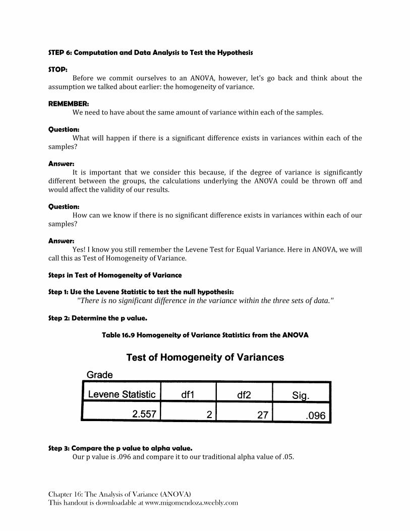
Yes! I know you still remember the Levene Test for Equal Variance. Here in ANOVA, we will call this as Test of Homogeneity of Variance. Steps in Test of Homogeneity of Variance Step 1: Use the Levene Statistic to test the null hypothesis:

"There is no significant difference in the variance within the three sets of data."

Step 2: Determine the p value.

Table 16.9 Homogeneity of Variance Statistics from the ANOVA

Step 3: Compare the p value to alpha value.

Our p value is .096 and compare it to our traditional alpha value of .05.




Step 4: Draw a conclusion. Since our p value is greater than our alpha value, this means we fail to reject our null

hypothesis. That is, there is no significant difference in the degree of variance within our three sets of data. Question:

What will happen if our p value was less than .05? Can we still use ANOVA? Answer:

If the p value was less than .05, hence we reject the null hypothesis we have for the test of homogeneity of variances. Thus, we might need to revert to the ANOVA's nonparametric equivalent; the Kruskal-Wallace H test. Keep in Mind:

The difference in the variances between the groups has to be very, very large in order for us to reject the null hypothesis for the test of homogeneity of variances, hence use Kruskal-Wallace H test.

Table 16.9 The Computation of Sums of Squares

𝑥1 𝑥12 𝑥2 𝑥2

2 𝑥3 𝑥32

80 84 90

82 86 92

78 84 94

76 82 90

80 88 100

72 90 94

82 92 94

88 88 96

74 86 92

68 84 94

∑ 𝑥1 = ∑ 𝑥12 = ∑ 𝑥2 = ∑ 𝑥2

2 = ∑ 𝑥3 = ∑ 𝑥32 =

Task 1:

Compute the Total Sum of Squares. Total Sum of Squares

1680.0000 Task 2:

Compute the Within Sum of Squares. Within Groups Sum of Square

460.8000 Task 3:

Determine the Between Sum of Squares.




Between Groups Sum of Squares 1,219.2000

Task 4:

Determine the degrees of freedom of between-groups. df of between-groups

2 Task 5:

Determine the degrees of freedom of within-group. df of within groups

27 Task 6:

Determine the total degrees of freedom. Total degrees of freedom

29 Task 7:

Compute the Between-Groups Mean Square. Computed Mean Square of Between Groups

609.600 Task 8:

Compute the Within-Group Mean Square. Computed Mean Square of Within Groups

17.067 Task 9:

Compute the F value. F Value

35.719 Task 10:

Determine the Critical F value. Critical F value:

3.35 Task 11:

Construct an F distribution, plot our F value and critical value of F, and make a intelligent conclusion.




Conclusion: Our computed value of F (i.e., 35.719) falls very far to the right of our critical value of F (i.e.,

3.35); there is a significant difference between the three groups. Task 12:

Test the Hypothesis using the p value.

Table 16.10 Inferential Statistics from the ANOVA.

Conclusion:

Our p value of .0000 (less than our alpha value of .05) tell us that there is a significant difference between the three groups. This supported our conclusion when we test our hypothesis using the F value and the critical value of F. Task 13:

Compute the value of Eta-Squared. Eta-Squared (Effect Size)

.726. Conclusion:

This value supports our decision. According to Cohen, we have a large effect size. STOP:

Here we have somewhat of a conundrum; we have rejected the null hypothesis and can feel assured that a significant difference exists between the groups. The questions that arise, however, are "Which groups are different? Is the CAI group different from Lecture? Is the Lecture group

different from Combination group? Is the Combination group different from the CAI group?

How can we figure this out?" Answer:

Yes, I know you still recall the Post-Hoc Test.

Lesson 16.12: The Post-Hoc Comparisons

As we said earlier, in order to determine which groups are significantly different, we could

use separate t-tests to compare the lecture and CAI groups, the lecture and combination groups, and the CAI and combination groups. Remember, however, that approach is not statistically sound.




This would mean that you would have a separate alpha value for each of the t-tests, which, of course, would greatly inflate the Type I error rate. Instead of doing that, we can use a set of tools called multiple comparison tests to help us make a more sound decision. The Multiple-Comparison Tests

These tests do exactly what their name implies. They make a comparisons between the levels of an ANOVA and tell us which are significantly different from one another. Note:

We won't get into the manual calculations; suffice it to say that they are a modified version of the independent t-test that controls for the inflated Type I error rate. Bonferroni Test

There are situations that require a specific multiple-comparison test, but these do not arise that often. For our purposes, one of the most commonly used multiple-comparison tests is the Bonferroni Test. The procedure is easy to understand, and it gives the researcher a good estimate of the probability that any two groups are different while, at the same time controlling for Type I and Type II errors.

Table 16.11 Multiple-Comparison Tests Following the ANOVA

Interpreting the Results of Multiple-Comparison Tests (Bonferroni Test) The Mean Difference

We can see here we are given statistics representing it and its relationship to the other levels of the independent variable. There is one quirk, however: because of the total number of possible comparisons, part of the table is redundant. Note:

The positive and negative sign doesn't matter. We take the absolute value and interpret these as they are. Meaning, greater than or less than differences exist.




The Asterisk Next to Each Mean Difference Value This indicates that the mean difference is significant when alpha equals .05.

The p Values

We can see the p value between each of these; this means the two groups in that given comparison are significantly different from one another. Again, the p value supports the significant difference shown by the asterisks next to all mean difference comparisons. Final Conclusion:

The use of a combination of lecture and CAI results in achievement scores significantly higher than either lecture alone or CAI alone. At the same time, the use of CAI is significantly more effective than the use of lecture alone. The teacher should use these information to plan future class sessions accordingly.

Let's Practice: Direction: Using the six-steps research model solve the given case below.

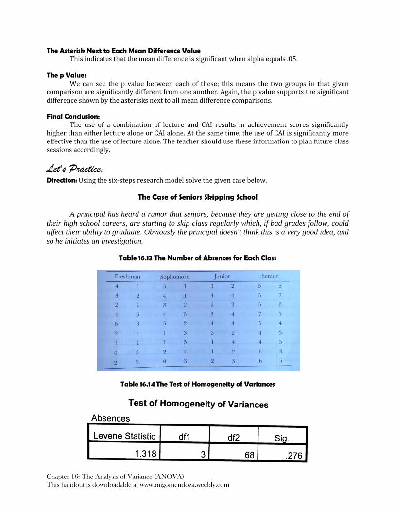
The Case of Seniors Skipping School

A principal has heard a rumor that seniors, because they are getting close to the end of

their high school careers, are starting to skip class regularly which, if bad grades follow, could

affect their ability to graduate. Obviously the principal doesn't think this is a very good idea, and

so he initiates an investigation.

Table 16.13 The Number of Absences for Each Class

Table 16.14 The Test of Homogeneity of Variances




Table 16.15 Multiple-Comparison Tests Following the ANOVA


chapter 16: the analysis of variance...

Documents