C H A P T E R

16

Advanced Reinforcement LearningNathaniel D. DawBox 16.1: Yael Niv

O U T L I N E

Introduction 299

The RL Formalism 300Markov Decision Processes 300Values, Policies, and Optimal Policies 300

Learning 301Learning Rules 301Learning Rates and Uncertainty 302

Rewards and Punishments 306The Subjectivity of Reward 306The Construction of Reward 306Punishment and Avoidance 307Dopamine and Punishment 307

States, Stimuli, and Perceptual Uncertainty 308Theory: Partial Observability and Perceptual

Inference 310From Perception to Decision 311POMDPs and Neuroscience 312

Actions 313Vigor, Opportunity Costs, and Tonic Dopamine 313Action Hierarchies, Action Sequences, and

Hierachical RL 314Multi-Effector Action 316

Conclusion 317

References 317

INTRODUCTION

This chapter takes a deeper look at reinforcementlearning (RL) theories and their role in neuroeco-nomics. The previous chapter described a prominentand well-studied hypothesis about a neural andcomputational mechanism for learning to chooserewarding actions, centered on the midbrain dopaminesystem and its targets, particularly in the striatum(Houk et al., 1995; Montague et al., 1996; Schultz et al.,1997). That chapter described how the phasic firing ofdopamine neurons appears to report a prediction errorthat would be appropriate for updating expectationsabout long-term future reward. It described the evi-dence that this signal may drive learning about actionpreferences, by affecting plasticity at synapses onto themedium spiny neurons of striatum, which have alsolong been believed to be involved in movement initia-tion and execution. Psychologically, as detailed inChapter 21, this mechanism appears to implement awell-studied category of behavior known as habitual

learning. Computationally, the dopamine responseclosely resembles the prediction error from temporal-difference (TD) learning, an algorithm for learnedoptimal control from computer science. Because of thiscorrespondence, this theory offers a direct line fromthe hypothesized neural and psychological mechan-isms to normative considerations about how an efficientagent should choose, a particularly important level ofunderstanding from a neuroeconomic perspective.

Working outward from the relatively secure core ofdopamine and TD learning, this chapter considersextensions and areas of current investigation. In partic-ular, after reviewing the RL theories in greater formaldetail than the preceding chapter, we consider a num-ber of problems that arise in matching up the theory’sabstract elements � learning updates, rewards, states,and actions � to more realistic ones relevant to anexperimental or real-world situation faced by a biologi-cal organism. We approach these questions startingfrom the normative, computational perspective � howan optimizing agent should learn � and in each case

299Neuroeconomics. DOI: http://dx.doi.org/10.1016/B978-0-12-416008-8.00016-4 © 2014 Elsevier Inc. All rights reserved.

review theory from the computational study of RL thatcan serve as a framework for conceptualizing how thebrain might approach the problem. In each of theseexamples, the resulting theory preserves the TD pre-diction error mechanism at the heart of a more com-plex and realistic account.

THE RL FORMALISM

Markov Decision Processes

We begin by detailing, more formally than in theprevious chapter, the problem solved by RL algorithmssuch as temporal-difference learning (Bertsekas andTsitsiklis, 1996; Sutton and Barto, 1998). Laying outthese formalisms will allow us to expose the corre-spondence between abstract elements of the theoryand aspects of real-world decisions by biologicalorganisms. Making different parts of this mappingbetween theory and experiment work raises a numberof questions and necessitates a number of elaborations,which are ultimately the topics of this chapter and ofmuch current research in neuroeconomics.

RL algorithms have primarily been developed(within computer science) to identify optimal decisionsin a formal class of tasks known as Markov decision pro-cesses (MDPs). MDPs are a class of decision-problemstripped down enough to be amenable to fairlystraightforward mathematical analysis, while still cov-ering a broad range of tasks and preserving a numberof the elements of nontrivial real world decisions. Thecore elements of an MDP are a set of situations orstates, S, and a set of actions, A, plus a specification oftransitions (how states and actions lead to other states)and rewards.

Within the framework of MDPs, the “world” haswhat are called discrete dynamics (as opposed to contin-uous time dynamics): The world’s state takes on a newvalue from S at each timestep, t (we write this as arandom variable st, st11, etc.). At each timestep, theagent also chooses an action at from A and receives areward rt, which measures the utility received on thattimestep. We take the reward to be a real number andassume that it is a function of the state and (for nota-tional simplicity) deterministic: rt5 r(st).

The actions are important because they influencethe evolution of the state, and hence the obtainedrewards. Specifically, the state at any time t1 1, st11, isa (probabilistic) function of the preceding state, st, andaction, at, determined by a transition distributionPðst11jst; atÞ. The most important simplifying assump-tion of the MDP � the Markov property for which it isnamed � is that this state transition probabilitydepends only upon the current state and action; condi-tional on these, the new state is independent of all

earlier states and actions. Rewards also obey theMarkov property, since they depend only on the cur-rent state and, conditional on this, are independent ofany earlier history. By constraining the relationshipsbetween events across time, the Markov conditionalindependence property simplifies analysis, learning,and decision making and is key to RL algorithms. (Inparticular, it allows formulating the Bellman equation,Equations 2 and 3 below.) But as we will discuss laterin the chapter, it also raises some difficulties relatingRL states to the sensory experiences of organisms,which typically do not obey the Markov property.

Despite these limitations, many decision tasks canbe characterized as MDPs, including Tetris, Americanfootball, and elevator scheduling (see Sutton andBarto, 1998, for many examples). Modeled as MDPs,different decision problems correspond to differentstate and action sets, and different transition andreward functions over them.

Values, Policies, and Optimal Policies

We are now in a position to evaluate decisionsbased on how much reward they obtain. As discussedin the previous chapter, the key complication fordecision making in this setting is that each action haslong-term consequences for the decision-maker’sreward prospects, via its influence on the successorstate, st11, and thence indirectly on all subsequentstates and rewards. Accordingly, just as a particularchoice of play in American football may not itself scorepoints but may set up field position that influencessubsequent scoring potential, to choose actions in anMDP we must take account of both the immediate anddeferred consequences of actions.

Let us define the decision variable � the quantitywe wish our choices to optimize � as the expectedcumulative, discounted future reward. This quantity,called the state-action value function, depends not onlyon the current state and action, but also on the actionswe take in subsequent states. First, let us define a pol-icy π(s) as any mapping from states to actions. Wewrite the value of taking an action in a state, and thenfollowing some policy π thereafter:

Qπðst; atÞ5E½rt 1 γrt11 1 γ2rt12 1 γ3rt13. . .jst; at;π�ð16:1Þ

Here, elaborating the similar equations in the previ-ous chapter, we have discounted future rewards expo-nentially in their delay by the discounting parameterγ# 1. We have also used the notation E½�jst; at;π� tostand in for the complicated expectation over all possi-ble future sequences of states and rewards given thestarting state and action, and the policy π.

300 16. ADVANCED REINFORCEMENT LEARNING

NEUROECONOMICS

We can make that expectation over future statesmore explicit by rewriting Equation 16.1 in recursiveform (the Bellman equation; Bellman, 1957):

Qπðst; atÞ5 rðstÞ1 γX

st11AS

Pðst11jst; atÞQπðst11;πðst11ÞÞ

ð16:2ÞThis form of the value function expresses the series of

rewards from Equation 16.1 as the first, r(st), plus all therest. The trick is that the cumulative value of “all therest” is also given by the value function, but evaluated atthe successor state st11. This value is discounted andaveraged over possible successors according to theirprobabilities. Thus the value function is defined in termsof the recursive relationship between the values at differ-ent states. See the previous chapter for a more detaileddiscussion of such recursions and their relevance to neu-roeconomics; our main goal here is to characterize whatit means to choose optimally in this setting.

Since the expected future value at each state is afunction of the policy π, we need to consider optimal-ity over policies rather than actions individually. As itturns out, for any MDP there exists at least one deter-ministic optimal policy π� which is globally best in thesense that at every state, its expected future rewardQ�ðs;π�ðsÞÞ is at least as good as that for any other pol-icy. (See, e.g., Puterman, 1994, for details.) We candefine the optimal value function, and its associatedpolicy, again recursively by using a form of theBellman equation that explicitly chooses the best actionin each state on the right side of the equation:

Q�ðst; atÞ5 rðstÞ1 γX

st11AS

Pðst11jst; atÞ maxat11AA

Q�ðst11; at11Þ

ð16:3Þ

The optimal policy, π�ðsÞ5 arg maxa½Q�ðs; aÞ�, is thengiven by the assignment, to each state, of the highest-valued action. That the optimal value function defines theoptimal policy is a formal instantiation of the intuitivestrategy of choosing actions by predicting their long-runrewards, which occupied much of the previous chapterand underlies much theorizing about the role of dopa-mine. After all, the difficulty in selecting actions in anMDP is that they have long-term effects. However, theseconsequences are exactly what the value functionQ� mea-sures. If you can learn it, then selecting the best action in astate is as simple as comparing its value between candi-dates and choosing the best.

In the rest of this chapter, we attempt to put elementsof this abstract theory back into a biological and psy-chological context. We begin with mechanisms for pre-diction learning, and then consider the real worldcounterparts of the main components of MDP’s:rewards, states, and actions.

LEARNING

Learning Rules

The basic strategy assumed by RL theories in neuro-science is that organisms learn state-action values bytrial and error, and use these as decision variables toguide choice. Starting from Equation 16.3, two impor-tant approaches present themselves.

The first is the one described in the previous chap-ter, and widely associated with dopamine. This is tomaintain internal estimates of Q(s, a) for all states andactions, and update these according to a temporal-difference prediction error (Sutton, 1988). We definethe prediction error as the extent Equation 16.3 fails tohold in a particular state-action-state sequence, by tak-ing the difference between the two sides of the equa-tion and replacing the expectation over possiblesuccessor states with the st11 actually observed:

δt 5 rt 1 γ maxat11AA

Qtðst11; at11Þ2Qtðst; atÞ ð16:4Þ

We can use this prediction error with the updaterule Qt11ðst; atÞ5Qtðst; atÞ1α � δt to improve our esti-mates, and ultimately (under various technical condi-tions) to converge on the true optimal values Q�. Thisversion of the algorithm is called Q-learning (Watkinsand Dayan, 1992). A few variations on this theme aresometimes seen in the literature. For instance, a relatedtemporal-difference algorithm called SARSA can bederived from the form of the Bellman equation inEquation 16.2, thereby replacing the max over actionsin Equation 16.4 with the action actually taken, inorder to learn the policy-specific rather than the opti-mal state-action values (Rummery and Niranjan, 1994).Another variant, called the actor-critic, is based on theBellman equation for the state value V (seeChapter 15), and learns both a state value functionVπðsÞ and a corresponding action selection policy π(s)(Barto, 1995). Here, the values and the policy are bothupdated by a temporal-difference prediction error sim-ilar to Equation 16.4. Importantly, all these threeapproaches share the essential strategy of learningtheir decision variables using a temporal-differenceprediction error based on some form of the Bellmanequation. (More can be learned about each in Suttonand Barto’s classic textbook, Sutton and Barto, 1998.)

Owing to their roots in the Bellman equation, thekey feature of these theories is that they use their ownestimates of the reward expected from a stateðQtðst11; at11Þ in Equation 16.4) to train the reward pre-dictions for the states that preceded it. As discussedextensively in Chapter 15, this feature, called bootstrap-ping, has a number of important echoes in behavioraland neural data, including the anticipatory responses

301LEARNING

NEUROECONOMICS

of dopamine neurons. Thus, although there have beensome efforts to distinguish which particular version ofthe temporal-difference prediction error best corre-sponds to the dopamine response (Morris et al., 2006;Roesch et al., 2007), the larger point is that the sort ofempirical and computational considerations discussedin the previous chapter connect the dopaminergic sys-tem to this family of RL algorithms. Collectively, thesealgorithms are known as model-free RL.

A distinctly different approach to RL, which doesnot involve prediction errors similar to dopaminergicresponses but may also be relevant in neuroeconomics,is to focus on learning the state transition and rewardfunctions, Pðst11jst; atÞ and r(st), which together definean MDP. This approach is called model-based RLbecause those two functions constitute an “internalmodel” or characterization of the task contingencies.Equation 16.3 defines the values Q� in terms of thesequantities (and Q�, in turn, defines the optimal policy),and so given the model you can use Equation 16.3 tocompute the values and derive a policy. The transitionand reward distributions are fairly straightforward tolearn: it is easy to directly observe an example of a one-step state transition or reward, and to average manysuch examples to estimate the functions. (In contrast,you can’t easily collect samples of long-run state-actionvalues Q since they accumulate rewards that unfoldover many steps. This is why learning Q directly via themodel-free methods above requires bootstrapping orother tricks.) The flip side of the simplicity in learningan internal model is computational complexity in usingit: in order to recover the predicted long-run values, itis necessarily to explicitly evaluate Equation 16.3. Tosee how this can be done, note that Q� is on both sidesof Equation 16.3; if you substitute the right hand side ofthe equation into itself for Q� repeatedly, you “unroll”the recursion into a series of nested sums taking expec-tations over the series of future states and rewards. Thestandard algorithm for computing values from the tran-sition and reward models, called value iteration, essen-tially corresponds to evaluating this expectationstepwise (Sutton and Barto, 1998).

Although model-free RL has received the majorityof attention in neuroscience, due to its relationshipwith the dopamine system, there has been an increas-ing understanding that the brain also uses model-based methods (Daw et al., 2005). This is the primarytopic of Chapter 21.

Note a confusing terminological issue: as used incomputer science and neuroscience � and in this book� the term “reinforcement learning” refers broadly tolearning in the context of decision problems, and com-prises many particular sorts of learning including boththe model-free and model-based approaches discussedabove. Economists, in contrast, sometimes use the term

“reinforcement learning” to refer more specifically toone particular approach to learning, essentially themodel-free strategy.

Learning Rates and Uncertainty

At the heart of model-free RL as used in theories ofdopamine is the concept of value learning by anerror-driven update, e.g. Qt11ðst; atÞ5Qtðst; atÞ1Qtðst; atÞ1αUδt. As discussed in Chapter 15, such a ruleseems sensible, at least informally: it fractionallynudges the prediction Q in the direction that reducesthe prediction error δ. But can we rationalize this proce-dure on more formal grounds? And in particular, canwe give some principled interpretation to the so-fararbitrary learning rate parameter α?

It is familiar in economics and computer science toframe learning in terms of statistical reasoning. On thisview, learning some quantity (here, Q) from a series ofnoisy observations is really just a statistical estimationproblem. That is, if we specify formal assumptionsabout the statistical structure of the noise, then ourestimates given our observations at each step (in effect,the learning rule) follow directly from the rules ofprobability (Dayan and Long, 1998). In particular,learning at each step requires combining what we pre-viously knew about the value with new evidence fromthe current observation. The rules of probability deter-mine how optimally to weight such sources of infor-mation when combining them, in effect, determiningthe appropriate step size α (Dayan et al., 2000; Kakadeand Dayan, 2002).

To flesh out how these ideas relate to error-drivenlearning, we sketch a statistical counterpart (Kakadeand Dayan, 2002) to the Rescorla�Wagner rule(Rescorla and Wagner, 1972; Equation 16.1 fromChapter 15) for classical conditioning. This is a simplerexample than TD in an MDP, but preserves many keyelements. In this setting, we encounter a series of trialsindexed k, each with a stimulus sk followed by an asso-ciated reward rk. We attempt to predict only the imme-diate reward given the state; here there is noaccumulation of predicted rewards across trials, whichis mainly what makes this example moretractable than the full MDP situation.

To reason statistically about this problem, we mustmake some assumptions about the noise. Assume thatthere is some true reward contingency, Vk(s), associ-ated with each stimulus, but that this is unknown andnot directly observed because the obtained rewardsare corrupted by Gaussian noise:

rk 5VkðskÞ1 εk ð16:5Þwhere εkBNð0;σrÞ.

302 16. ADVANCED REINFORCEMENT LEARNING

NEUROECONOMICS

Set up this way, the problem of reward prediction isjust the problem of noisy measurement. If I have previ-ously observed a number of rewards following stimu-lus, s, then I can estimate Vk(s), but only up to alimited degree of accuracy (conversely, with someuncertainty) due to the measurement noise. One way tocharacterize such uncertainty is as a distribution, whichassigns a probability (e.g., a degree of belief) to eachpossible value of V being the correct one conditionalon the previously observed stimuli and rewards. Theestimation problem here is constructed to ensure thatthese distributions will take the form of Gaussians, i.e.,at each step, for each stimulus, s, we can expressPðVkðsÞjo1. . .ok21; s1. . .sk21Þ as NðμkðsÞ;σkðsÞÞ.

The distribution (formally, the posterior distribution)describing our estimates about V has both a meanvalue μkðsÞ, and a variance σ2

kðsÞ, the latter characteriz-ing uncertainty as the spread of belief away from themean. This approach therefore generalizes the sorts oflearning rules we have considered thus far to accountexplicitly for uncertainty about the learned estimate.

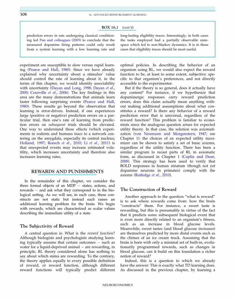
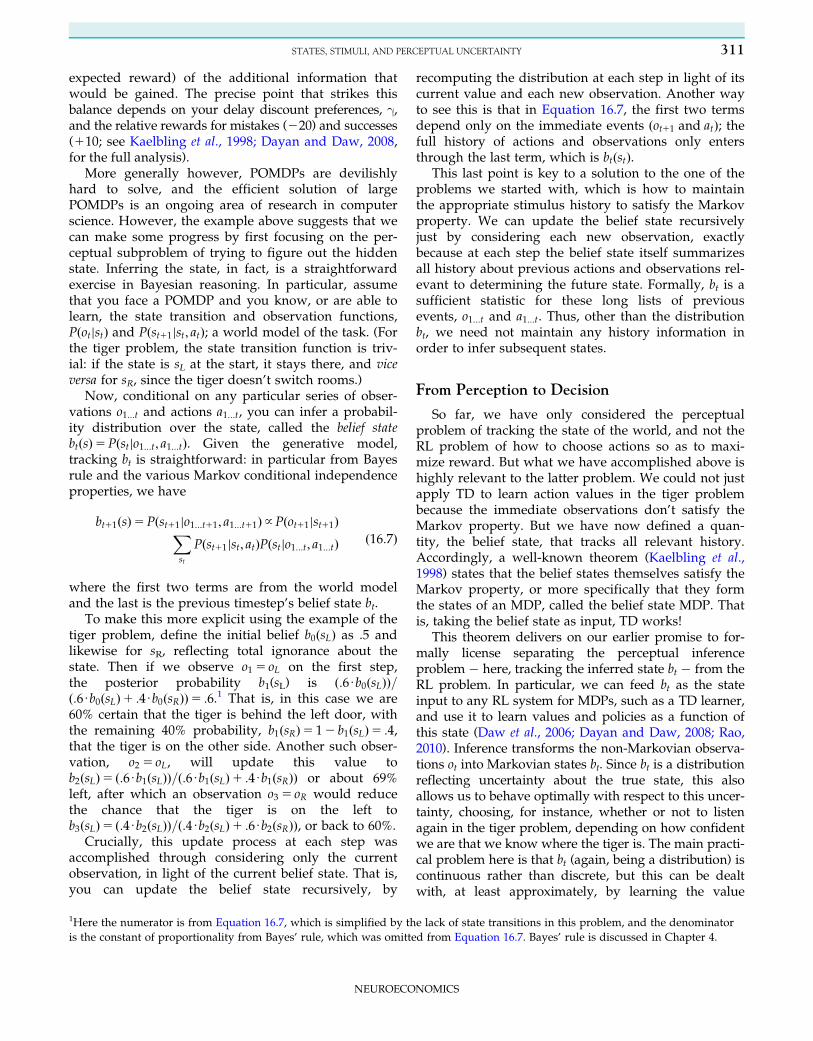
If we now observe a new trial with a stimulus sk andreward rk, then the new posterior distribution overVk(sk) is given by the laws of probability, specificallyBayes’ rule. We are combining two uncertain sources ofinformation about the value, one being the previousestimate, and the other (from Equation 16.5) the new,noisy measurement. Intuitively, the weight given toeach of these information sources in determining theupdated posterior depends on their relative uncertainty(Figure 16.1). If I was sure already, a single noisy mea-surement won’t move my belief much; conversely, ifthe measurement is much more precise than my previ-ous beliefs, then it will largely replace them. This is an

instance of a principle of Bayesian cue combination thatis also prominent in other areas of psychology, such asperception, where it is often used to describe optimalcombination between different modalities such asvision and audition (Knill and Pouget, 2004).

Formally, applied to this problem, Bayes’ rule (togetherwith identities for manipulating Gaussian distributions)implies update equations for the mean and variance ofour posterior distribution given each new observation.Strikingly, the rule for the mean estimate, μkðskÞ takesexactly the familiar form of an error-driven update:μk11ðskÞ5μkðskÞ1κkUδk, with prediction errorδk 5 rk 2μk.

It is worth stopping to consider what we have accom-plished here. We have just produced a rational derivationjustifying from first principles the sort of error-drivenlearning rule that is widely hypothesized in neuroeco-nomics on more empirical grounds. More importantly,this derivation sheds additional light on the problembecause the new variable κk, plays the role of the learningrate α, but is no longer an arbitrary, free parameter.Instead, its value can be computed from Bayes’ rule as:

κk 5σ2kðskÞ

σ2kðskÞ1 σ2

r ðskÞð16:6Þ

which reflects a comparison between the relative uncer-tainty of the previous beliefs, σ2

kðskÞ, and the “noisiness”(or variability) in the rewards, σ2

r ðskÞ (from Equation16.5).

Equation 16.6 makes explicit the intuition fromFigure 16.1: the learning rate is maximal when uncer-tainty about the value is high relative to small noise inthe observed rewards, and the opposite situation

FIGURE 16.1 Bayesian cue combination weights evidence sources by their uncertainty. The blue and green Gaussians represent the distri-bution over the true value given by the previous evidence and the new observation, respectively. Each distribution has a mean (the verticaldashed line) and uncertainty, expressed as a variance around that mean. The posterior distribution arising from combining the two, in red,has a mean that interpolates between the two source means. These are weighted according to their uncertainty, such that if the two evidencesources are equally reliable (A) the resulting mean is their average, but if one is more uncertain than the other (B) the posterior mean is shiftedtoward the more reliable estimate.

303LEARNING

NEUROECONOMICS

results in low learning rates. The qualitative relation-ship illustrated here between uncertainty and learningrates is very general, though quantitatively fleshingout similar probabilistic approaches in other learningproblems such as action value estimation in MDPs isquite complex (Dearden et al., 1998; Daw et al., 2005;Behrens et al., 2007). In fact, it is important to stressthat many real world problems, even those quite closeto the “toy problem” described here can beintractable to this kind of analysis for what are largelytechnical reasons.

The theoretical dependence of the learning rate onthe outcome noise, from Equation 16.6, may have acounterpart in the prediction error-related responses ofdopamine neurons. Although dopamine neurons willgenerally respond more for larger unexpected rewards(i.e., larger prediction errors) this response scales rela-tive to the range of rewards expected (Tobler et al.,2005). In fact, the response to a small reward can beindistinguishable from that for a large reward, so longas both occur at the top of their respective ranges. Oneway to understand this effect (due to Preuschoff andBossaerts, 2007) is to assume that the neurons reportnot the raw prediction error δk but instead the predic-tion error scaled by the learning rate, κkUδk, which is,anyway, the quantity that should ultimately controlthe amount of plasticity at recipient structures. Therange of rewards can be thought of as correspondingto the outcome noise σ2

r ðskÞ, which scales the learningrate through Equation 16.6, and in this way would nor-malize the modeled dopaminergic responses.

The recognition of the key role of uncertainty, notjust for controlling learning rates but for probabilisticreasoning in many other areas of perception and cog-nition, has driven a sustained but so far still reason-ably speculative interest in possible mechanisms bywhich the brain may represent and manipulate uncer-tainties (Yu and Dayan, 2005; Ma et al., 2006).

So far we have considered the update rule only forthe mean of the value distribution. In the relativelysimple example given here, the corresponding updaterule for the uncertainty (variance) of the posterior isnot very interesting: uncertainty starts high anddeclines toward zero as you collect more observations,leading to a decaying learning rate. However, thedynamics of uncertainty in more elaborate inferenceproblems have a number of interesting psychologicalcounterparts.

An important case arises if the true reward contin-gencies Vk(s) are not stationary, but instead changeover time, as is typical in the laboratory and likelyoften the case in real-world learning � for foraginganimals different food patches may deplete andreplenish, for animals in a lab experiment block tran-sitions may shift the contingencies sporadically.

A simple statistical assumption about such change(but one not justified in most laboratory environ-ments) is that the true values fluctuate from trial-to-trial according to Gaussian random walks. Togetherwith Equation 16.5, this assumption leads to a modelcalled the Kalman filter (Kalman, 1960; Sutton, 1992;Kakade and Dayan, 2002). Here, the possibility thatthe values have changed between trials contributesadditional uncertainty to the posterior distribution ateach step, ensuring that the learner never becomesentirely certain about a stimulus’ current value. Thisleads, asymptotically, to uncertainty stabilizing at thelevel where the information coming in (due to eachobservation) matches that “lost” due to the ongoingnoisy change in the true values, in turn making thelearning rate κk asymptotically constant over trials.These considerations clarify the constant learning rateoften assumed in RL models: it is appropriate(asymptotically) in a non-stationary task of this sort.

A benefit of this kind of theoretical exercise is that itgrounds a previously arbitrary parameter � the learn-ing rate � in objective, experimentally manipulableand measurable aspects of the environment. Forinstance, in the Kalman filter, the level at which thelearning rate asymptotes depends on the amount oftrial�trial change in the true values (their volatility:the variance of their random walk), because this con-trols the asymptotic posterior uncertainty σ2

kðskÞ inEquation 16.6. Intuitively, the faster the value beinglearned is changing, the less relevant is previous expe-rience (relative to new experience) in inferring its cur-rent value, so higher learning rates should be used toplace more weight on new observations. This predic-tion has been tested and confirmed in RL experimentswith humans, in which volatility was manipulated(Behrens et al., 2007).

These last results, finally, point to the issue ofmetalearning, or estimating the parameters such asthe volatility and outcome noise, which shoulddetermine uncertainty and learning rates. TheKalman filter takes these as given (e.g., the outcomenoise appears as a constant in Equation 16.6), butsubjects clearly have to learn them as well. This ispossible by further elaborating statistical modelsin the spirit of the one described above to includean additional level of inference about the noiseparameters. Following this approach, Behrens andcolleagues. (2007) constructed trial-by-trial timeseriesreflecting subjects hypothesized learning about valuevolatility and report that these covary with BOLDsignals in the anterior cingulate cortex.

The relationship between learning rates and envi-ronmental volatility may also have a counterpart inan older literature from psychology on associability orthe degree to which different stimuli in a conditioning

304 16. ADVANCED REINFORCEMENT LEARNING

NEUROECONOMICS

BOX 16.1

E L IG I B I L I TY TRACES

B y Ya e l N i v

Eligibility traces (Barto et al., 1981; Sutton and Barto,

1998) are a computational construct that is perhaps eas-

ier to justify from a biological, real-world learning per-

spective than from a theoretical one. The main idea is

that every state that is visited by the agent or animal can

remain eligible for updating for a certain period of time,

so that prediction errors due to several forthcoming

rewards and state transitions (and not just the immedi-

ate ones) can modify the state’s value. In this way, a

reward can easily modify the value of states and actions

that occurred in the not-immediately recent past, allow-

ing learning even with delayed outcomes.

In practice, rather than committing to a timeframe of

eligibility, one can set an eligibility “trace” e(s) that

decays exponentially over time:

ek11ðsÞ5 1 for s5 sk ðthe current stateÞek11ðsÞ5λekðsÞ for all other states s 6¼ sk

(and similarly for state-action pairs). At each timestep,

the values of all states are updated according to the pre-

diction error multiplied by the state’s eligibility trace,

such that some states are “more eligible” for updating

than others. The scheme above is what Sutton & Barto

termed “replacing traces” as the trace for the visited

state becomes 1, replacing its previous value. Another

option is to add 1 to the (λ-decayed) previous trace of

the visited state, thus generating “accumulating traces”

(Sutton and Barto, 1998).

Temporal difference learning with eligibility traces is

termed TD(λ), after the parameter that governs the

decay of the eligibility trace, which must be between 0

and 1. At one extreme, if λ5 0 we get standard temporal

difference learning (also known as TD(0)), as the current

state is the only state eligible for updating at each time-

step. At the other extreme of TD(1) (also known as Full

Monte Carlo Learning), on every timestep all states that

have ever been visited are updated, a scheme that is

equivalent to using the full return (all the future

rewards) to update the value of a state. These TD var-

iants are all normative, that is, under the right condi-

tions on learning rate and sampling, they can be shown

to converge on the correct state values (Sutton and

Barto, 1998). In general, the TD(λ) algorithm can be

viewed as (exponentially) averaging learning with

different-horizon returns, with the shorter returns being

weighted more strongly. Thus the “forward view” of eli-

gibility traces sees the traces as a mechanism that allows

learning from future rewards. An equivalent “backward

view” sees eligibility traces as a mechanism that allows

each reward to affect not only the just-visited state, but

also those states visited in the recent past (with

“recency” decaying exponentially; Killeen, 2011).

In practice, eligibility traces can be seen as a memory

mechanism that helps bridge gaps between events. This

is extremely convenient for learning in the real world, as

eligibility traces allow learning even if the state space is

not strictly Markov (Loch and Singh, 1998; Singh et al.,

1994): values can be updated correctly even if non-

Markov states intervene between an action and its con-

sequences (Todd et al., 2009). Consider, for instance, a

classic trace-conditioning experiment: a rat sits in an

experimental chamber for a length of time, then on some

occasions a light turns on, turns off, and after two sec-

onds a food pellet is delivered to the rat. The state of the

world in which the rat is sitting in the box with no light

on is thus ambiguous: if this state occurs before any

light has turned on, the rat has little reason to expect

reward to follow this state. However, if this state occurs

after the light on state, the rat should expect that reward

is forthcoming. Unless the rat represents these two

situations as two unique states, the task is not a

Markov one. Specifically, the occurrence of the inter-

vening no light state will impair the rat’s ability to learn

to predict reward as a result of the light turning on.

The light on state will be followed by a state that has

low value (as it frequently leads to nothing) and thus

will not acquire high value as befitting a situation that

leads to reward with 100% certainty. However, with

eligibility traces, it is clear that the value of the light on

state will be updated to reflect the upcoming reward,

suffering only from a learning rate that is reduced by a

factor of λ.The neuroscience of eligibility traces is rather

straightforward: states can remain eligible for updating

through prolonged activity of neurons representing a

certain state (Seo et al., 2007), and/or through any form

of synaptic tagging that marks recently active synapses

for future plasticity through LTP or LTD (Izhikevich,

2007), for instance, elevated levels of calcium in the den-

dritic spines of medium spiny neurons (Wickens and

Kotter, 1995). Indeed, eligibility traces have been pro-

posed to be integral to cerebellar learning (Wang et al.,

2000; McKinstry et al., 2006). Bogacz and colleagues

found behavioral evidence for eligibility traces in data

from humans performing a decision-making task

(Bogacz et al., 2007), and an analysis of dopaminergic

305LEARNING

NEUROECONOMICS

experiment are susceptible to slow versus rapid learn-ing (Pearce and Hall, 1980). Since we have alreadyexplained why uncertainty about a stimulus’ valueshould control the rate of learning about it, in theterms of this chapter, we would identify associabilitywith uncertainty (Dayan and Long, 1998; Dayan et al.,2000; Courville et al., 2006). The key findings in thisarea are the many demonstrations that animals learnfaster following surprising events (Pearce and Hall,1980). These results go beyond the observation thatlearning is error-driven. Instead, if one experienceslarge (positive or negative) prediction errors on a par-ticular trial, then one’s rate of learning from predic-tion errors on subsequent trials should be elevated.One way to understand these effects (which experi-ments in rodents and humans trace to a network cen-tering on the amygdala, especially its central nucleus;Holland, 1997; Roesch et al., 2010; Li et al., 2011) isthat unexpected events may increase estimated vola-tility, which increases uncertainty and therefore alsoincreases learning rates.

REWARDS AND PUNISHMENTS

In the remainder of this chapter, we consider thethree formal objects of an MDP � states, actions, andrewards � and ask what they correspond to in the bio-logical setting. As we will see, in each case, these con-structs are not static but instead each raises anadditional learning problem for the brain. We beginwith rewards, which are characterized as scalar valuesdescribing the immediate utility of a state.

The Subjectivity of Reward

A central question is: What is the reward function?Although biologists and psychologists studying learn-ing typically assume that certain outcomes � such aswater for a liquid-deprived animal � are rewarding, inprinciple, RL theory considered alone has nothing tosay about which states are rewarding. To the contrary,the theory applies equally to every possible definitionof reward, or reward function, although differentreward functions will typically predict different

optimal policies. In describing the behavior of anorganism using RL, we would also expect the rewardfunction to be, at least to some extent, subjective: spe-cific to that organism’s preferences, and not directlyaccessible to the experimenter.

But if the theory is so general, does it actually haveany content? For instance, if we hypothesize thatdopaminergic responses carry reward predictionerrors, does this claim actually mean anything with-out making additional assumptions about what con-stitutes a reward? Is there any behavior of a rewardprediction error that is universal, regardless of thereward function? This problem is familiar to econo-mists since the analogous question arises for expectedutility theory. In that case, the solution was axiomati-zation (von Neumann and Morgenstern, 1947; seeChapter 1): the choices of an expected utility maxi-mizer can be shown to satisfy a set of basic axioms,regardless of the utility function. There has been asimilar program to recast parts of RL in axiomaticform, as discussed in Chapter 1 (Caplin and Dean,2008). This strategy has been used to verify thatBOLD responses in human striatum (though not yetdopamine neurons in primates) comply with theaxioms (Rutledge et al., 2010).

The Construction of Reward

Another approach to the question “what is reward”is to ask where rewards come from: how the brain“constructs” them. For instance, a sweet taste isrewarding, but this is presumably in virtue of the factthat it predicts some subsequent biological event thatis even more directly related to an organism’s fitness,such as an increase in blood glucose levels.Meanwhile, sweet tastes (and blood glucose increases)are themselves predicted by more distal events such asthe chimes of an ice cream truck. Assuming that thebrain is born with only a minimal set of built-in, evolu-tionarily programmed rewards, such as changes inblood glucose, can it build on this foundation a richernotion of reward?

Indeed, this is a question to which we alreadyhave the answer: This is exactly what TD learning does.As discussed in the previous chapter, by learning a

BOX 16.1 (cont’d)

prediction errors in rats undergoing classical condition-

ing led Pan and colleagues (2005) to conclude that the

measured dopamine firing patterns could only result

from a system learning with a low learning rate and

long-lasting eligibility traces. Interestingly, in both cases

the tasks employed had a partially observable state-

space which led to non-Markov dynamics. It is in these

cases that eligibility traces should be most useful.

306 16. ADVANCED REINFORCEMENT LEARNING

NEUROECONOMICS

long-run future value function over states, TD learns totreat stimuli that are predictive of future events alreadyspecified as rewards in many ways equivalently to theultimate rewards themselves. TD learns to assign highvalues to states that predict future reward; whenencountered unexpectedly, these drive reward predic-tion error (and the assignment of value to still more dis-tal states that predict them), just like primary rewards.As stressed in Chapter 15, this device explains how thebrain comes to value secondary reinforcers such asmoney. Exactly the same principle would allow thebrain to learn that sweet tastes are rewarding (assum-ing, for the sake of the example, this is not itself inbuilt)because they reliably predict subsequent, slow changesin blood glucose. Thus, fundamental to these theories isan account how the brain builds up a rich landscape ofvalue given a minimal seed.

Punishment and Avoidance

Perhaps the largest set of open questions in thisarea concerns how to treat punishments in this frame-work. In principle, aversive events could just beassigned negative reward values and assessed on acommon scale together with rewards. Indeed, tradi-tional economic models begin with this assumption.Psychology suggests that aversive processing may besomewhat more complicated, however. Whereas thedopamine system clearly represents a common path-way for many different sorts of appetitive stimuli, it isless clear to what extent aversive stimuli (or costs) arealso integrated into the dopaminergic signal. Early ani-mal conditioning experiments (such as counter-conditioning, in a which stimulus is trained to predictboth reward and punishment) led to the suggestionthat appetitive and aversive predictions are actuallymaintained in separate, opponent channels rather thanstored as a single net value summing over positiveand negative (Konorski, 1967; Solomon and Corbit,1974).

One neural constraint that may motivate thisapproach is that the firing rates of neurons arebounded below by zero, meaning that they map mostnaturally onto half of the real line; positive or negativenumbers rather than both. This constraint is thought togive rise to opponent representations in other situa-tions such as color vision. For RL, the low backgroundfiring rates of dopamine neurons suggest a limiteddynamic range for reporting unexpected punishmentsif they are simply coded as negative rewards, sinceexcursions below the baseline are rectified at zero fir-ing rate (though see Bayer et al., 2007). It has been sug-gested, albeit on quite indirect evidence, that parts ofthe ascending serotonin system might serve as an

aversive opponent to dopamine, carrying the otherhalf of the signal (Daw et al., 2002).

A related question with a long history in animalconditioning is how responses for avoiding (or escap-ing) punishment are learned and motivated.Psychological theory suggests that the termination ofpunishment, or more importantly the cessation of theexpectation of punishment, can be reinforcing (Maia,2010; Mowrer, 1951; Moutoussis et al., 2008), enablingavoidance learning. Cues predicting danger, but alsosuccessful avoidance, can also come to be associatedwith anticipated relief or safety (D’amato et al., 1968)as well as danger. For instance, a cue may signal theaversive expectancy that an electric shock is imminent,but if that shock can be avoided (e.g., by a lever press),then the cue additionally signals the opportunity foravoidance, a relative improvement. Relief and its antic-ipation can only be relatively positive (relative to pun-ishment and its anticipation) � the net value of anavoided punishment is clearly nil � but in the contextof opponent systems, the negative aspects of fear andthe opposing positive aspects of relief might be codedseparately, activating both positive and negativechannels.

Dopamine and Punishment

Given all this psychological and computational com-plexity, it is perhaps not surprising that there havebeen conflicting reports how dopamine neuronsbehave in response to punishments and stimuli pre-dicting punishment. Although some dopaminergicunits are inhibited by these events, or unresponsive(Matsumoto and Hikosaka, 2009; Mirenowicz andSchultz, 1996; Ungless et al., 2004) � consistent withthe expectation that they are coded as negativerewards, or separately � there have been reports ofother putatively dopaminergic neurons that are excitedby aversive stimuli as well as rewarding ones (Joshuaet al., 2008; Matsumoto and Hikosaka, 2009).

One recent report argued that there were two clas-ses of putatively dopaminergic neurons: one showingthe classic prediction error response, and the otherexcited both by signals of future punishment andreward (Matsumoto and Hikosaka, 2009). In general,a failure to differentiate good from bad outcomesseems hard to explain from the perspective of netdecision variables, and for this reason such responseshave tended to be understood in terms of arousal orattention rather than reinforcement (Horvitz, 2000).However, as mentioned, rather than the net overreward and punishment, dopamine might preferen-tially report the positively motivating aspects ofanticipated relief from danger, due to avoidance

307REWARDS AND PUNISHMENTS

NEUROECONOMICS

(Maia, 2010; Moutoussis et al., 2008) in the context ofa system where the accompanying aversive aspectsare coded elsewhere. Regarding avoidance, many lab-oratory experiments in this area have used noxiousairpuff stimuli to the face or eye, which typically can-not be avoided entirely but may be mitigated some-what by blinking. In any case, the suggestedheterogeneity of dopamine response types also cutsagainst the concept of the dopaminergic response as aunitary, scalar prediction error (see Chapter 15) andcomplicates the problem of interpreting the dopami-nergic signal at the recipient structures.

Most confusingly, the interpretation of all theseresults depends importantly on the methods used toclassify recorded neurons as dopaminergic. Typically,in extracellular recordings, this classification is basedon characteristics of the extracellular responses such asthe spike width and the background firing rate, fea-tures which are known (originally from more invasiveintracellular recordings with verified histology) to bepredictive of dopaminergic status. However, dopami-nergic neurons are intermixed with other, nondopami-nergic neurons, and at least in some dopaminergicregions these electrophysiological properties do notperfectly discriminate neuronal types (Margolis et al.,2006; Ungless and Grace, 2012; Ungless et al., 2004).

There are, however, more technically elaborate tech-niques that can be used to identify neurons that syn-thesize dopamine and these explicitly dopaminergicneurons can be examined in detail. When dopaminer-gic status is verified, false positive rates (neurons thatwould be wrongly characterized as dopaminergicusing electrophysiological criteria) in the rat ventraltegmental area are typically higher than 10% and inone study nearly 40% (Ungless and Grace, 2012).

This brings us back to the question of punishmentresponsiveness. In one study that used juxtacellularand immunofluorescent labeling to verify conclusivelythe presence of dopamine in recorded neurons, all truedopaminergic neurons were found to be inhibited bypunishment and all the neurons that were excited bypunishment were found to be nondopaminergic neu-rons that would have been misclassified as dopaminer-gic if electrophysiological properties alone had beenused, as is almost always the case in primate studies(Ungless et al., 2004). Another study that tagged dopa-mine neurons optogenetically detected small responsesto punishment in verified dopaminergic neurons onlyat a low rate similar to that expected due to chance(Cohen et al., 2012). A third study reported verifieddopamine neurons that were indeed excited by pun-ishment, but these were relatively segregated in a con-strained anatomical location (the ventral part of theventral tegmental area) (Brischoux et al., 2009).Confusingly, the punishment-responsive neurons from

the primate study by Matsumoto and Hikosaka (2009)tended to be located toward the opposite end of themidbrain (dorsolateral substantia nigra pars compacta)from the punishment-responsive dopaminergic neu-rons identified in rodents by Brischoux and colleagues(2009), suggesting the importance of future directstudy of these neurons using methods that can achievepositive identification of dopaminergic biochemistry.

STATES, STIMULI, AND PERCEPTUALUNCERTAINTY

The most stylized and unrealistic aspect of the MDPmodel is the state. In an MDP, the world has a state stat each timestep, which determines its subsequentdynamics. In order to use standard RL approaches tosolve the MDP, the agent needs to know that state: inthe parlance of computer science, the state must befully observable. Standard RL approaches rely on theMarkov property that, conditional only on the currentstate and action, all future states and rewards are inde-pendent of everything that happened previously. Thismeans that to solve the RL problem in an MDP, theagent need not “remember” any previous states: onlythe currently observed one matters. Coming at thesame point from the other direction, if an agent is solv-ing a task using standard RL algorithms, then what-ever the agent uses as its state must contain all historyabout previous events that is relevant to predictingsubsequent states and rewards.

What could this state correspond to in a biologicalorganism? Clearly, in part, it includes the animal’songoing perceptual sensations, but as we will see theseare typically insufficient to satisfy the Markov propertyby themselves: the real world is not an MDP, at leastone in which the states correspond directly to percepts.Instead, we must identify the RL state with an internalrepresentation comprising not only immediate percep-tual sensations, suitably analyzed and processed, butalso interoceptive ones (e.g., motivational states suchas hunger that indicate which future outcomes will berewarding) and working memories (of whatever previ-ous stimuli are relevant to future rewards). It mayseem that embedding working memories into theagent’s state is a trick allowing the agent to use theMDP approach even in a world that is not really anMDP. And of course that is exactly what it is.

The important point here is thus that several hetero-geneous cognitive functions can be hidden behind theseemingly simple notation st. On the other hand, thatmay be a fairly realistic feature of this class of models.The dopamine neurons and their striatal afferents areinterconnected with the frontal lobes and hence, bymost obvious routes, many synapses away from the

308 16. ADVANCED REINFORCEMENT LEARNING

NEUROECONOMICS

sense organs. That is if st is the RL system’s input �the thing that it maps to value predictions and predic-tion errors � then it may well be reasonable to envi-sion this input as a highly processed quantity, arrivingby way of the brain’s whole cortical machinery for per-ceptual analysis. (That said, there are also some impor-tant shortcuts, notably direct connections from pre-cortical sensory areas of the colliculus to the midbraindopamine neurons, which are thought to play a role inshort-latency dopamine responses to sensory events;Dommett et al., 2005.)

Below, we will consider approaches which separatethe problem of constructing a state � perceptual analy-sis � from the reinforcement learning problem itself,with the former “module” providing the input to thelatter. As we will see below, researchers in computerscience have, in effect, argued that mathematical fea-tures of the problem license this separation of function.More practically, as we will also see, existing work oncortical mechanisms for perceptual inference fits thebill well in terms of complementing the RL system aswe have already described it here and in the precedingchapter.

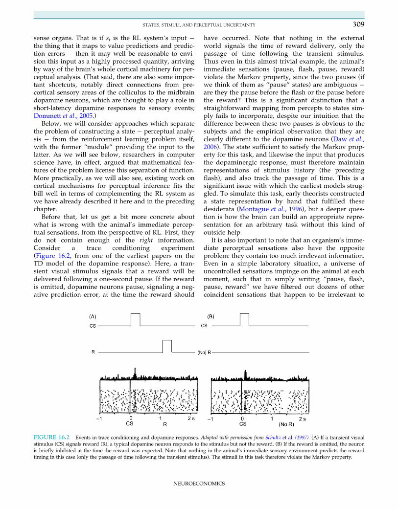
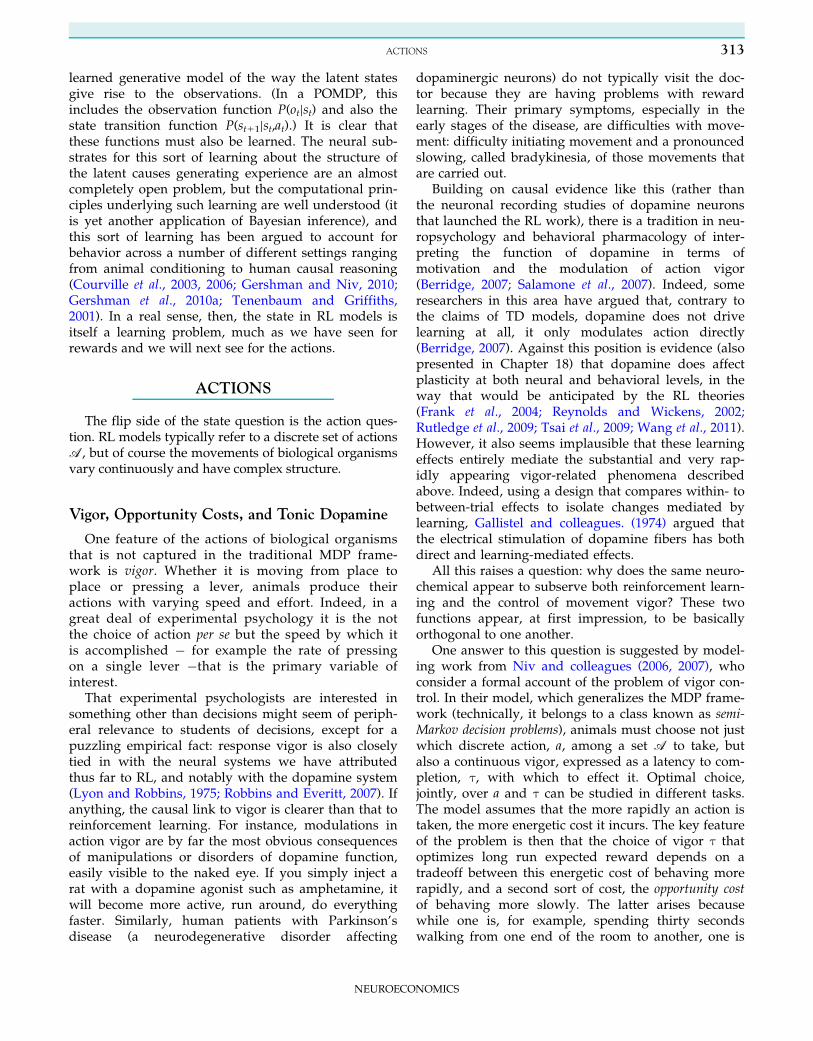
Before that, let us get a bit more concrete aboutwhat is wrong with the animal’s immediate percep-tual sensations, from the perspective of RL. First, theydo not contain enough of the right information.Consider a trace conditioning experiment(Figure 16.2, from one of the earliest papers on theTD model of the dopamine response). Here, a tran-sient visual stimulus signals that a reward will bedelivered following a one-second pause. If the rewardis omitted, dopamine neurons pause, signaling a neg-ative prediction error, at the time the reward should

have occurred. Note that nothing in the externalworld signals the time of reward delivery, only thepassage of time following the transient stimulus.Thus even in this almost trivial example, the animal’simmediate sensations (pause, flash, pause, reward)violate the Markov property, since the two pauses (ifwe think of them as “pause” states) are ambiguous �are they the pause before the flash or the pause beforethe reward? This is a significant distinction that astraightforward mapping from percepts to states sim-ply fails to incorporate, despite our intuition that thedifference between these two pauses is obvious to thesubjects and the empirical observation that they areclearly different to the dopamine neurons (Daw et al.,2006). The state sufficient to satisfy the Markov prop-erty for this task, and likewise the input that producesthe dopaminergic response, must therefore maintainrepresentations of stimulus history (the precedingflash), and also track the passage of time. This is asignificant issue with which the earliest models strug-gled. To simulate this task, early theorists constructeda state representation by hand that fulfilled thesedesiderata (Montague et al., 1996), but a deeper ques-tion is how the brain can build an appropriate repre-sentation for an arbitrary task without this kind ofoutside help.

It is also important to note that an organism’s imme-diate perceptual sensations also have the oppositeproblem: they contain too much irrelevant information.Even in a simple laboratory situation, a universe ofuncontrolled sensations impinge on the animal at eachmoment, such that in simply writing “pause, flash,pause, reward” we have filtered out dozens of othercoincident sensations that happen to be irrelevant to

FIGURE 16.2 Events in trace conditioning and dopamine responses. Adapted with permission from Schultz et al. (1997). (A) If a transient visualstimulus (CS) signals reward (R), a typical dopamine neuron responds to the stimulus but not the reward. (B) If the reward is omitted, the neuronis briefly inhibited at the time the reward was expected. Note that nothing in the animal’s immediate sensory environment predicts the rewardtiming in this case (only the passage of time following the transient stimulus). The stimuli in this task therefore violate the Markov property.

309STATES, STIMULI, AND PERCEPTUAL UNCERTAINTY

NEUROECONOMICS

the task. The problem of learning is the problem ofgeneralization from previous experiences to the cur-rent one. If st is defined so exhaustively that the animalnever encounters the same state twice, then learningcan’t get off the ground.

A third problem with perceptual sensations is thatthey are often ambiguous. Many tasks in perceptioncome down to drawing uncertain inferences fromnoisy measurements � was there a rustle? Where didthat sound come from? Is that a tiger in the bushes?Indeed, even the simple example of trace conditioningimplicates perceptual uncertainty, because the subjec-tive perception of the passage of time is noisy. Thus,if a stimulus is followed in one second by reward,and the stimulus has been observed but reward hasnot been received, the subject will face uncertainty asto whether the full second has already elapsed or isstill ongoing, and thus uncertainty whether thereward was omitted or is still to arrive (Daw et al.,2006).

In short, to make TD work, the brain needs to con-struct a state representation that contains adequatehistory, omits irrelevant information, and somehowcopes with perceptual uncertainty. And that is moreof a challenge than might be immediately obvious.

Theory: Partial Observability and PerceptualInference

A standard way of characterizing some of thesesorts of problems in computer science is a formalismknown as the partially observable MDP (POMDP),which augments the MDP with an explicit characteri-zation of noisy perception (Kaelbling et al., 1998). APOMDP is just an MDP, with the exception that thestate st is hidden or not observable to the agent, whoinstead receives at each step some noisy observation otrelated to the state. The observation is determined bythe hidden state, according to some distributionPðotjstÞ, but the mapping may be stochastic and theobservation may not uniquely identify the state. Notethat although the hidden states obey the Markov prop-erty by assumption, the observations need not (andgenerally will not) do so. A violation of the Markovproperty means that the current observation is insuffi-cient to predict future states and rewards, and thus tosolve a POMDP, unlike an MDP, it is necessary to takeaccount of previous observations as well. The distinc-tion between the states and the observations allowsPOMDPs to characterize problems like trace condition-ing, in which the immediate stimuli are too sparse toobey the Markov property, as well as problems inwhich violations of the Markov property arise due tonoisy perception.

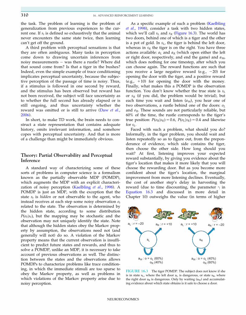
As a specific example of such a problem (Kaelblinget al., 1998), consider a task with two hidden states,which we’ll call sL and sR (Figure 16.3). The world hastwo doors, behind one of which is a tiger and the otheris a pot of gold. In sL, the tiger is behind the left door,whereas in sR the tiger is on the right. You have threeactions available: aL and aR (which open either the leftor right door, respectively, and end the game) and aW,which does nothing for one timestep, after which youcan choose again. The reward functions are such thatyou receive a large negative reward (e.g., 220) foropening the door with the tiger, and a positive reward(e.g., 110) for opening the door with the money.Finally, what makes this a POMDP is the observationfunction. You don’t know whether the true state is sLor sR (if you did, the problem would be trivial), buteach time you wait and listen (aW), you hear one oftwo observations, a rustle behind one of the doors: oLand oR. These sounds are not particularly reliable, but60% of the time, the rustle corresponds to the tiger’strue position: PðoRjsRÞ5 0:6; PðoLjsRÞ5 0:4 and likewisefor sL.

Faced with such a problem, what should you do?Informally, in the tiger problem, you should wait andlisten repeatedly so as to figure out, from the prepon-derance of evidence, which side contains the tiger,then choose the other side. How long should youwait? At first, listening improves your expectedreward substantially, by giving you evidence about thetiger’s location that makes it more likely that you willchoose the rewarding door. But as you become moreconfident about the tiger’s location, the marginalimprovement from more listening declines. Eventually,the cost of another step’s delay in harvesting thereward (due to time discounting, the parameter γ inEquation 16.3 and discussed in more detail inChapter 10) outweighs the value (in terms of higher

aL : r = –20

aW : o = oL (60%)oR (40%)

aW : o = oL (40%)oR (60%)

aR : r = –20aR : r = +10

sL sR

aL : r = +10

FIGURE 16.3 The tiger POMDP. The subject does not know if sheis in state sL, where the left door aL is dangerous, or state sR, wherethe right door aR is dangerous. Only by waiting (aW) and accumulat-ing evidence about which state obtains is it safe to choose a door.

310 16. ADVANCED REINFORCEMENT LEARNING

NEUROECONOMICS

expected reward) of the additional information thatwould be gained. The precise point that strikes thisbalance depends on your delay discount preferences, γ,and the relative rewards for mistakes (220) and successes(110; see Kaelbling et al., 1998; Dayan and Daw, 2008,for the full analysis).

More generally however, POMDPs are devilishlyhard to solve, and the efficient solution of largePOMDPs is an ongoing area of research in computerscience. However, the example above suggests that wecan make some progress by first focusing on the per-ceptual subproblem of trying to figure out the hiddenstate. Inferring the state, in fact, is a straightforwardexercise in Bayesian reasoning. In particular, assumethat you face a POMDP and you know, or are able tolearn, the state transition and observation functions,PðotjstÞ and Pðst11jst; atÞ; a world model of the task. (Forthe tiger problem, the state transition function is triv-ial: if the state is sL at the start, it stays there, and viceversa for sR, since the tiger doesn’t switch rooms.)

Now, conditional on any particular series of obser-vations o1...t and actions a1...t, you can infer a probabil-ity distribution over the state, called the belief statebtðsÞ5Pðstjo1...t; a1...tÞ. Given the generative model,tracking bt is straightforward: in particular from Bayesrule and the various Markov conditional independenceproperties, we have

bt11ðsÞ5Pðst11jo1...t11; a1...t11Þ~Pðot11jst11ÞXst

Pðst11jst; atÞPðstjo1...t; a1...tÞ ð16:7Þ

where the first two terms are from the world modeland the last is the previous timestep’s belief state bt.

To make this more explicit using the example of thetiger problem, define the initial belief b0ðsLÞ as .5 andlikewise for sR, reflecting total ignorance about thestate. Then if we observe o1 5 oL on the first step,the posterior probability b1(sL) is ð:6Ub0ðsLÞÞ=ð:6Ub0ðsLÞ1 :4Ub0ðsRÞÞ5 :6.1 That is, in this case we are60% certain that the tiger is behind the left door, withthe remaining 40% probability, b1ðsRÞ5 12 b1ðsLÞ5 :4,that the tiger is on the other side. Another such obser-vation, o2 5 oL, will update this value tob2ðsLÞ5 ð:6Ub1ðsLÞÞ=ð:6Ub1ðsLÞ1 :4Ub1ðsRÞÞ or about 69%left, after which an observation o3 5 oR would reducethe chance that the tiger is on the left tob3ðsLÞ5 ð:4Ub2ðsLÞÞ=ð:4Ub2ðsLÞ1 :6Ub2ðsRÞÞ, or back to 60%.

Crucially, this update process at each step wasaccomplished through considering only the currentobservation, in light of the current belief state. That is,you can update the belief state recursively, by

recomputing the distribution at each step in light of itscurrent value and each new observation. Another wayto see this is that in Equation 16.7, the first two termsdepend only on the immediate events ðot11 and atÞ; thefull history of actions and observations only entersthrough the last term, which is btðstÞ.

This last point is key to a solution to the one of theproblems we started with, which is how to maintainthe appropriate stimulus history to satisfy the Markovproperty. We can update the belief state recursivelyjust by considering each new observation, exactlybecause at each step the belief state itself summarizesall history about previous actions and observations rel-evant to determining the future state. Formally, bt is asufficient statistic for these long lists of previousevents, o1...t and a1...t. Thus, other than the distributionbt, we need not maintain any history information inorder to infer subsequent states.

From Perception to Decision

So far, we have only considered the perceptualproblem of tracking the state of the world, and not theRL problem of how to choose actions so as to maxi-mize reward. But what we have accomplished above ishighly relevant to the latter problem. We could not justapply TD to learn action values in the tiger problembecause the immediate observations don’t satisfy theMarkov property. But we have now defined a quan-tity, the belief state, that tracks all relevant history.Accordingly, a well-known theorem (Kaelbling et al.,1998) states that the belief states themselves satisfy theMarkov property, or more specifically that they formthe states of an MDP, called the belief state MDP. Thatis, taking the belief state as input, TD works!

This theorem delivers on our earlier promise to for-mally license separating the perceptual inferenceproblem � here, tracking the inferred state bt � from theRL problem. In particular, we can feed bt as the stateinput to any RL system for MDPs, such as a TD learner,and use it to learn values and policies as a function ofthis state (Daw et al., 2006; Dayan and Daw, 2008; Rao,2010). Inference transforms the non-Markovian observa-tions ot into Markovian states bt. Since bt is a distributionreflecting uncertainty about the true state, this alsoallows us to behave optimally with respect to this uncer-tainty, choosing, for instance, whether or not to listenagain in the tiger problem, depending on how confidentwe are that we know where the tiger is. The main practi-cal problem here is that bt (again, being a distribution) iscontinuous rather than discrete, but this can be dealtwith, at least approximately, by learning the value

1Here the numerator is from Equation 16.7, which is simplified by the lack of state transitions in this problem, and the denominator

is the constant of proportionality from Bayes’ rule, which was omitted from Equation 16.7. Bayes’ rule is discussed in Chapter 4.

311STATES, STIMULI, AND PERCEPTUAL UNCERTAINTY

NEUROECONOMICS

function of bt using methods for approximating continu-ous functions.

POMDPs and Neuroscience

The theory of POMDPs helps to clarify what weneed out of a state representation for a TD system, andin particular casts the rather ill-defined problem ofproducing an appropriate state representation in theterms of a well-defined Bayesian inference problem.This is useful for a number of reasons; most impor-tantly it reveals a rather clean correspondence betweenwhat the brain needs from the perspective of solvingthe RL problem, and what theoretical neuroscientistsstudying perception have already suggested that thebrain’s sensory systems provide. The idea that the jobof the brain’s sensory systems is essentially to recon-struct the hidden causes underlying noisy percepts is alongstanding one in neuroscience (often traced back toHelmholtz, 1860). The framework of Bayesian genera-tive modeling and inference underlies prominent mod-ern views of perception (Knill and Pouget, 2004; Yuilleand Kersten, 2006), such as models that explain thereceptive fields of V1 neurons as detecting latent fea-tures common in natural images (Lewicki andOlshausen, 1999; Olshausen, 1996).

An even more direct line exists between thePOMDP problem as described here, and recent workon the brain’s substrates for judgments about noisyperceptual stimuli (Gold and Shadlen, 2002; Roitmanand Shadlen, 2002; Yang and Shadlen, 2007). In neuro-science, this research is considered to fundamentallybe about decision making, though this work is largelydisjoint from research on RL and other classes of moreeconomic decision making, because the focus is pri-marily on perceptual uncertainty rather than optimiz-ing utility. For the same reason, however, the twokinds of decision-making studies in neuroscience arequite complementary. The tiger problem described inthe previous section is a standard example of aPOMDP from computer science, but it is also isomor-phic to a well-studied task in perceptual neuroscience,the dots judgment task of Newsome and colleagues, dis-cussed in Chapters 8 and 19 (Newsome and Pare,1988). The task requires judging whether a partiallycoherent motion stimulus is moving left or right. Here,the tiger task’s states sL and sR correspond to the possi-ble motion directions, and the observations representinstantaneous morsels of perceived motion energy.A line of research by Shadlen and colleagues charac-terizes the pre-saccadic responses of neurons in lateralintraparietal area LIP as accumulating evidence aboutmotion direction, captured in their model (Gold andShadlen, 2002) as a transformed version of the POMDP

belief state, log(bt(sL)/bt(sR)). There is a direct relation-ship between this belief state’s evolution and thedynamics of a drift diffusion process of the kind oftenused to model this class of tasks, and discussed indetail in Chapter 3.

At least as characterized in these experiments, this sys-tem is thus a direct example of a neural representation ofexactly the sort of belief state we have argued is necessaryfor TD to solve the policy optimization part of this task,i.e., learning under what circumstances to respond “left”or “right”. (That said, this specific neural population hasadditional properties that make it an imperfect candidatefor a pure representation of belief state, notably that itsneurons are also modulated by saccade utility; Platt andGlimcher, 1999.) In any case, the composition of belieftracking and TD models predicts some non-trivial beha-viors of the downstream reward prediction error signal asa result of upstream perceptual uncertainty, such asslowly unfolding positive or negative errors reflecting theinference that a particular motion stimulus is easier orharder than expected (Rao, 2010). Such responses haveindeed been observed in primate dopamine neuronsrecorded during the dots judgment task (Nomoto et al.,2010). Using a very different task in rodents, the lesion oforbitofrontal cortex produced a pattern of changes in theresponses of dopamine neurons, which modeling sug-gested was consistent with the elimination of internallygenerated (i.e., not externally stimulus-bound) aspects ofthe TD system’s state representation (Takahashi et al.,2011). This result led the authors to suggest that the OFC,which is upstream from ventral striatum and dopamineneurons of the ventral tegmental area, might be contribut-ing to the state representation.

Behaviorally, learning and choice behavior inanother RL task with a hidden state is well explainedas resulting from such a hybrid scheme of combiningBayesian inference of the latent state with TD for learn-ing action values over the inferred state (Gershmanet al., 2010b). This task (see also Wilson and Niv, 2011)requires choice between options that are identified bya number of stimulus dimensions (color, shape, etc.).At any particular time, only one dimension is diagnos-tic as to which option is rewarding, and the other fea-tures are distractors. This task thus captures another ofthe state representation problems we began this sectionwith: the profusion of irrelevant stimuli. This problemof dimensional selective attention admits exactly thesame sort of solution, in terms of Bayesian inferenceabout the hidden state, as the other problems we haveconsidered, because in this task the true generativemodel contains only one relevant stimulus and infer-ence over the hidden state therefore serves to highlightit and suppress the others.

A final point is that, as described in the previoussection, inferring the latent state in the task requires a

312 16. ADVANCED REINFORCEMENT LEARNING

NEUROECONOMICS

learned generative model of the way the latent statesgive rise to the observations. (In a POMDP, thisincludes the observation function P(otjst) and also thestate transition function P(st11jst,at).) It is clear thatthese functions must also be learned. The neural sub-strates for this sort of learning about the structure ofthe latent causes generating experience are an almostcompletely open problem, but the computational prin-ciples underlying such learning are well understood (itis yet another application of Bayesian inference), andthis sort of learning has been argued to account forbehavior across a number of different settings rangingfrom animal conditioning to human causal reasoning(Courville et al., 2003, 2006; Gershman and Niv, 2010;Gershman et al., 2010a; Tenenbaum and Griffiths,2001). In a real sense, then, the state in RL models isitself a learning problem, much as we have seen forrewards and we will next see for the actions.

ACTIONS

The flip side of the state question is the action ques-tion. RL models typically refer to a discrete set of actionsA, but of course the movements of biological organismsvary continuously and have complex structure.

Vigor, Opportunity Costs, and Tonic Dopamine

One feature of the actions of biological organismsthat is not captured in the traditional MDP frame-work is vigor. Whether it is moving from place toplace or pressing a lever, animals produce theiractions with varying speed and effort. Indeed, in agreat deal of experimental psychology it is the notthe choice of action per se but the speed by which itis accomplished � for example the rate of pressingon a single lever �that is the primary variable ofinterest.

That experimental psychologists are interested insomething other than decisions might seem of periph-eral relevance to students of decisions, except for apuzzling empirical fact: response vigor is also closelytied in with the neural systems we have attributedthus far to RL, and notably with the dopamine system(Lyon and Robbins, 1975; Robbins and Everitt, 2007). Ifanything, the causal link to vigor is clearer than that toreinforcement learning. For instance, modulations inaction vigor are by far the most obvious consequencesof manipulations or disorders of dopamine function,easily visible to the naked eye. If you simply inject arat with a dopamine agonist such as amphetamine, itwill become more active, run around, do everythingfaster. Similarly, human patients with Parkinson’sdisease (a neurodegenerative disorder affecting

dopaminergic neurons) do not typically visit the doc-tor because they are having problems with rewardlearning. Their primary symptoms, especially in theearly stages of the disease, are difficulties with move-ment: difficulty initiating movement and a pronouncedslowing, called bradykinesia, of those movements thatare carried out.

Building on causal evidence like this (rather thanthe neuronal recording studies of dopamine neuronsthat launched the RL work), there is a tradition in neu-ropsychology and behavioral pharmacology of inter-preting the function of dopamine in terms ofmotivation and the modulation of action vigor(Berridge, 2007; Salamone et al., 2007). Indeed, someresearchers in this area have argued that, contrary tothe claims of TD models, dopamine does not drivelearning at all, it only modulates action directly(Berridge, 2007). Against this position is evidence (alsopresented in Chapter 18) that dopamine does affectplasticity at both neural and behavioral levels, in theway that would be anticipated by the RL theories(Frank et al., 2004; Reynolds and Wickens, 2002;Rutledge et al., 2009; Tsai et al., 2009; Wang et al., 2011).However, it also seems implausible that these learningeffects entirely mediate the substantial and very rap-idly appearing vigor-related phenomena describedabove. Indeed, using a design that compares within- tobetween-trial effects to isolate changes mediated bylearning, Gallistel and colleagues. (1974) argued thatthe electrical stimulation of dopamine fibers has bothdirect and learning-mediated effects.

All this raises a question: why does the same neuro-chemical appear to subserve both reinforcement learn-ing and the control of movement vigor? These twofunctions appear, at first impression, to be basicallyorthogonal to one another.

One answer to this question is suggested by model-ing work from Niv and colleagues (2006, 2007), whoconsider a formal account of the problem of vigor con-trol. In their model, which generalizes the MDP frame-work (technically, it belongs to a class known as semi-Markov decision problems), animals must choose not justwhich discrete action, a, among a set A to take, butalso a continuous vigor, expressed as a latency to com-pletion, τ, with which to effect it. Optimal choice,jointly, over a and τ can be studied in different tasks.The model assumes that the more rapidly an action istaken, the more energetic cost it incurs. The key featureof the problem is then that the choice of vigor τ thatoptimizes long run expected reward depends on atradeoff between this energetic cost of behaving morerapidly, and a second sort of cost, the opportunity costof behaving more slowly. The latter arises becausewhile one is, for example, spending thirty secondswalking from one end of the room to another, one is

313ACTIONS

NEUROECONOMICS

not otherwise earning reward. In fact, during that timeone is, in a real sense, delaying all subsequent rewardsthat might be earned after crossing the room.

In the analysis done by Niv and colleagues (2006,2007), this opportunity cost takes a simple form:2τUr,where r is the average reward per timestep. That is ifone takes a monetary example; if on average you couldbe earning $10 per minute, then every minute spentwalking across the room is $10 foregone. If you couldbe earning $100 per minute, your sloth is all the morecostly, and you face increased incentive to walk fasterso as to return more rapidly to earning money. Acrossmany tasks, this effect is reflected directly in the opti-mal choice of τ: you should behave more rapidly inenvironments where the average reward r is higher,since in this case the opportunity costs of inactionweigh more strongly against the energetic costs of vig-orous action. This analysis has an interesting counter-part in classic work in optimal foraging theory, wherethe optimal time to leave a diminishing patch of foodalso depends on r due to a similar opportunity costargument (Charnov, 1976; Stephens and Krebs, 1987).

The foregoing modeling provides a rational analysisof response vigor, and through the construct of theopportunity cost, grounds it in the reward rate.Experiments have indeed shown that manipulations ofreward rate affect response vigor (Guitart-Masip et al.,2011; Haith et al., 2012). The role of the reward ratealso suggests an answer to why dopamine is involvedin the vigor problem as well as the RL problem, as inthe case of bradykinesia in Parkinson’s disease(Mazzoni et al., 2007). To understand why, considerthe TD error, δt 5 rt 1Qtðst11; at11Þ2Qtðst; atÞ. (Here,compared to Equation 16.4, we have set γ5 1 and usedthe SARSA form of the rule, the version that omits the‘max0’operation.) This is a standard model, from theRL perspective, of the phasic responses of dopamineneurons. Note that if you sum (or, equivalently, aver-age) the prediction error δt over a range of timestepst5 [1, 2, 3, . . .], the terms involving the predictions Qcancel each other pairwise, since the same prediction isadded at one timestep and subtracted at the next.Whatever the predictions, then, in TD learning thesum of prediction errors over time is essentially justthe sum of rewards.

The upshot of all this is that implicit in the TD errorsignal is the average reward r: it is just the predictionerror response viewed in the aggregate over a longertimescale. This observation led Niv and colleagues(2006, 2007) to speculate that whereas phasic dopamineresponses (the high frequency bursts and abruptpauses in action potential rate) have been argued tocarry δt, the same dopamine signal viewed at a tonic(lower frequency) timescale might report the averagereward r. They further suggested, due to the

relationship between opportunity cost and optimalvigor, that this tonic dopamine signal should beexpected causally and directly to modulate responsevigor, which would tie in and explain the behavioralpharmacology results with which this section began.

The most straightforward mechanistic proposal,given the above considerations, may be to associate theaverage reward with extrasynaptic (see Chapter 5)dopamine concentrations in the striatum. Like otherneurotransmitters, dopamine is released into synapses,but dopamine is substantially present in the extracellu-lar fluid as well. This is because rather than releasingtheir transmitter only at terminal synapses located atthe ends of their axons, dopamine neurons containlarge numbers of release sites (called en passant synap-ses) throughout their extensive axonal trees. Theseallow each neuron to release dopamine throughout alarge volume of the recipient brain, where it escapesthe local synaptic cleft and diffuses through the extra-cellular fluid (Arbuthnott and Wickens, 2007). Thiseffect is particularly prominent following phasic dopa-minergic responses (as for prediction errors) in experi-ments using voltammetric methods (see Chapter 6),which observe transient increases in extrasynapticdopamine concentration (Garris et al., 2002; Phillipset al., 2003). The resulting extrasynaptic dopamine canaffect striatal medium spiny neurons via high-affinitydopamine receptors that are located away from thesynapses. Altogether, it is tempting to hypothesize thatthese transients, temporally filtered by diffusion andreuptake, give rise, in effect, to an averaging operationby which the baseline extracellular concentrationtracks the average reward r. Of course, reality may bemore complicated; for instance, there is evidence thatextrasynaptic levels of dopamine in striatum (at leastas tracked by microdialysis, a technique for directchemical sampling at a very slow temporal resolutionof one sample per 10 minutes) are regulated indepen-dently from phasic firing (Floresco et al., 2003).

Leaving aside the exact mechanism by which theaverage reward is computed, the Niv et al. (2006, 2007)model brings response vigor under the purview ofrational RL theories, and poses one possible answer tothe question of why the functions of vigor and RL arenaturally, almost necessarily, interconnected.

Action Hierarchies, Action Sequences, andHierachical RL

Another problem with mapping the actions A in anRL model to the real world is that it’s not clear what levelof granularity they are supposed to describe. In laboratoryexperiments an animal might face a choice between look-ing at a red or a green target, which (appear to) map

314 16. ADVANCED REINFORCEMENT LEARNING

NEUROECONOMICS

straightforwardly onto the simple theories discussedabove. However, consider the problem of driving a car,which is something most of us have learned to do.

How would we describe driving as an MDP(Sutton, 1995)? At one level, the set of actions mightrefer to maneuvers like changing lanes, drivingstraight, or turning left or right. But to execute each ofthese maneuvers, one needs to carry out differentsequences of lower-level actions, operating the pedalsand the steering wheel, and in turn to do each of thesethings by moving muscles. Conversely, at a higherlevel of analysis one might describe actions like follow-ing Interstate 76 to Exit 33 and then followingHighway 376 west to the end. These navigationalactions each require extended sequences of turning,tracking lanes and so on. In principle, one coulddescribe a navigational problem as an MDP withactions at any of these levels of granularity � steeringwheels, right turns, or highway exits. As this exampleshows, action in realistic environments seems to havea natural hierarchical structure: more abstract actionsare composed from more elemental actions. Suchabstraction can clearly simplify the choice and learningproblems: one cannot (plausibly) plan a road trip fromNew York to San Francisco in terms of the sequence ofoperations on the vehicle controls. At the same time,the lower level is essential: one cannot execute such atrip without ultimately operating the steering wheeland pedals.

What action space do the brain’s putative RL sys-tems learn over, then? The implausibility of planningroad trips in the space of vehicular controls meansthat if they work only in the “natural” space of move-ments of the body, we would (literally) never get any-where. Moreover, analogous interpretationalproblems occur even in a seemingly simple laboratoryproblem like choosing between two colored targets,since at a lower level even that abstract choice needsto be expressed through a series of movements withsome effector, such as a saccadic eye movement or abutton press.

In computer science, these issues have been studiedin an area known as hierarchical RL (Barto andMahadevan, 2003; Parr and Russell, 1998; Sutton et al.,1999), and more recently these ideas have beenbrought to neuroscience by Botvinick and colleagues(2009). Using one popular approach, the optionsframework, much of the RL machinery we have dis-cussed can be applied over a hierarchical action space,in which higher level actions (known as options) standin for extended sequences of lower level actions, andthis decomposition may be extended hierarchically(Sutton et al., 1999). Thus, at an intermediate level ofdescription, one might choose to make a left turn (anoption); at a lower level, a controller for the left turn

option has the responsibility to execute the maneuver,by making a series of choices about how to turn thewheel and press the pedals to pursue this goal.Decomposing the action space in this way also decom-poses the RL problem into a hierarchy of simpler ones:at the higher levels, the existence of the left turn optionsimplifies the learning problem by enabling the systemto neglect the microstructure of the maneuver, whereasthe left turn controller can also, separately, be trainedby its own, local, RL process targeted to its own goals.

Hierarchical RL then, seems like a plausible frame-work for solving the action problem in models of RLin the brain, explaining how the action space can bebuilt up from simple bodily movements to bridgethem to the more abstract sorts of relevant to labora-tory experiments or real-world decisions (Botvinicket al., 2009). As for how hierarchical RL works, there isreally one relevant fact, which is that it still workswith TD learning.

To be more precise, in hierarchical RL there aremultiple learning problems at different levels, and allof them can be solved by TD learning (or indeed, alter-natively by model based RL, or any mixture of theseacross levels). At the highest level, one still needs tochoose what to do so as to maximize reward, andapart from some accounting for options that take timeto complete, this works much as before. But makingchoices over abstract options sloughs off another partof the learning problem, which is that the option con-trollers (turning left or right) also need to be able tolearn to execute their respective maneuvers as effi-ciently as possible. The key point is that these subsidi-ary learning problems (known as intra-option learning:learning how to complete an option) can each them-selves be framed as RL problems and each also solvedwith TD methods. The main difference is that theoption controllers should learn as though they areattempting to optimize a different reward, the pseudore-ward that they attain by completing their respectivesubgoals, such as completing the turn. Thus they havedifferent different (pseudo) reward prediction errors,giving rise to different value functions, but via thesame learning rule (Figure 16.4).

All this suggests that the same sorts of computa-tional and neural mechanisms already described canachieve learning at multiple levels of an action hierar-chy, and together produce a more realistic account ofwhat “actions” are (Botvinick et al., 2009). The basalganglia mechanisms associated with RL seem wellsuited to subserve such a hierarchy, since the samepatterns of connections with cortex and with dopa-mine are repeated across many different (and appar-ently reasonably segregated) “loops” through the basalganglia, connected topographically to different areas offrontal cortex (Alexander and Crutcher, 1990). It has

315ACTIONS

NEUROECONOMICS

been suggested that a hierarchical controller could belaid out with actions at different levels of abstractionrepresented at different positions along this topogra-phy (Bornstein and Daw, 2011; Dezfouli and Balleine,2012; Frank and Badre, 2012; though see Chapter 21for a discussion of evidence supporting a differentorganizational scheme for these loops). One challeng-ing aspect of such a hypothesis is that different levelsof the action hierarchy require training from different(reward versus pseudoreward) prediction error sig-nals. If these are all to be carried by dopamine, differ-ent dopaminergic responses would have to beheterogeneous and segregated between the levels. Thiscuts somewhat against the impression (see Chapter 15)of dopamine as a strikingly diffuse and homogeneousbroadcast signal. Anatomically, the connectionsbetween dopamine neurons and striatum, though dif-fuse, have at least some topographical organizationthat might in principle support a coarse hierarchy(Haber et al., 2000), but dopamine neurons have notyet been examined in tasks with hierarchical structureto see if any heterogeneity in their responses emerges.

In any case, more broadly consistent with the hierar-chical RL idea, in an RL task involving hierarchicalaction, BOLD responses in the human striatum covarywith the size of positive prediction errors related tochanges in expectation about subgoal attainment: thatis, with the pseudoreward prediction errors hypothe-sized to be used to train the option controller (Ribas-Fernandes et al., 2011). (These results, and similarresults using EEG, were obtained at times in the taskwhen the top-level prediction error for primary rewardwas zero.) There is also fMRI evidence suggesting thatneural topography respects a related notion of actionhierarchy, whereby response rules with differentdegrees of nested contingent structure recruit distinctfrontal and striatal areas along a posterior�anterioraxis (Badre et al., 2010; Badre and Frank, 2012). Finally,a line of unit recording studies in rodent dorsolateralstriatum has shown that neurons there (but not, for

instance, in adjacent dorsomedial striatum) have a sortof “action chunking” property (Jog et al., 1999; Thornet al., 2010). As an animal learns a task involving aseries of actions to navigate a T-maze, different neu-rons in the population initially respond to differentevents along the route, but with more training, theneurons come to respond only to the beginning andend of the trial. This may reflect the coding of theentire action chain as a unit, like an option.

Both empirically and theoretically, a major questionin this area � the so-called option discovery problem � ishow the hierarchies get set up in the first place; how auseful set of subgoals can itself be learned from experi-ence. (This is different from the intra-option learningproblem, which can be addressed using TD: how bestto attain a given subgoal, such as changing lanes.)There is relatively little guidance on this problem fromthe computational literature, since this is substantiallyan open problem in computer science as well.

Multi-Effector Action

A related problem of hierarchy in action, also relevantto biology, is the problem of multi-effector action. Thebody has many effectors � two hands, two legs, and soon. If we treat the elemental actions A of an RL systemas combinations of movements of each of the effectors,then the high dimensionality of the effector space leadsto an exponential explosion in the set of candidateactions. This is a classic “curse of dimensionality” andwould complicate choice and learning. Another area ofhierarchical RL considers learning over high-dimensional action spaces of this sort, as with choosingactions for each member of a team of soccer-playingrobots or a fleet of fishing boats (Chang et al., 2003;Rothkopf and Ballard, 2010; Russell and Zimdars, 2003).The main strategy here is to divide and conquer, decom-posing the intractable high dimensional problem into anumber of smaller ones involving only subsets of

s1

Qtop(s1,a)

a s2

Qtop(s2,o)

o

s3

Qopt(s3,a)

a s4

Qopt(s4,a)

a s5

Qopt(s5,a)

s6

Qtop(s6,a)

a

a

pr

rδδ

δ δ

FIGURE 16.4 Prediction errors in hierarchical RL, after Botvinick et al. (2009). At the top level, the system may choose either a normalaction a or an extended option o. The latter choice transfers control to the option, which chooses more actions. Each level is learning its ownaction value estimates, Qtop or Qopt, predicting reward r or pseudoreward pr, respectively. These learning problems each involve separatereward (or pseudoreward) prediction errors.

316 16. ADVANCED REINFORCEMENT LEARNING

NEUROECONOMICS

effectors considered in isolation. This strategy seemswell suited to many natural actions � think of talkingon the phone while you walk � basically independentactions involving non-overlapping sets of effectors.

Perhaps more importantly, because the brain’smovement systems are organized topographically, theyare also well situated to treat choice over different effec-tors’ movements separately from one another. Indeed,this view is implicit in the interpretation of, for instance,activity of neurons in lateral intraparietal cortex as avalue map over saccade targets and the medial intrapar-ietal cortex as a value map over arm movements (Plattand Glimcher, 1999; see Chapter 20). Such a representa-tion reduces the multi-effector learning problem to mul-tiple, simpler RL problems in each effector separately.If they were learning simultaneously, they would alsorequire multiple prediction errors. Accordingly, in anfMRI study, distinct prediction errors were seen in leftand right striatum for movements of the contralateralhand, in a task where these had separable values(Gershman et al., 2009; see also Palminteri et al., 2009;Wunderlich et al., 2009). Finally, of course, if the brain isorganized to separate choice between effectors bydefault, this leads to a new problem of coordination:how to solve tasks like playing the piano or touch typ-ing that require the conjoint action of multiple effectors.In this case the value of (for example) a particular handmovement may depend on what the other hand does,and in such a task these values cannot be represented inseparate value maps for each hand. Although there is aclassic literature on coordination in movements, espe-cially across the hemispheres (Brinkman, 1984; Laplaneet al., 1977; Tanji et al., 1988), from a neuroeconomic per-spective, the valuation and decision problems overcoordinated multi-effector actions are so far largelyunstudied.

CONCLUSION

Like all models in science, the TD theory of thedopamine response is stylized and simplified. Thischapter has examined a number of these simplifica-tions and argued that in each of these cases, the theo-ry’s core mechanism for error driven learning can beused to address these additional problems. Thus, forinstance, error-driven learning is still called for whenthe update rule is derived from principles of statisticalmeasurement; the belief states in a POMDP form anMDP that can be solved with TD learning; and learn-ing at multiple levels of an action hierarchy can alltake place according to a common TD mechanism.

A related goal of this chapter was to lay the computa-tional foundations for dealing with problems like statesand actions in the context of RL theories, in part by

examining how these problems have been treated incomputer science. From a neuroeconomic perspective,one of the most important aspects of the TD theory is thatit connects the hypothesized neural mechanism to precisenormative considerations about learned optimal choice,based on the same decision theoretic principles thatunderlie economic analyses of these problems. The addi-tional computational frameworks presented here � forexample POMDPs and hierarchical RL � are not, as yet,so deeply developed in terms of their biological under-pinnings. However, they provide a promising theoreticalfoundation for investigating these issues neuroscientifi-cally, particularly because they dovetail so closely withthe relatively well studied TD machinery. In this respect,finally, it is worth noting that due to the rapid turn-around of human neuroimaging experiments, many ofthe newer ideas discussed here have been investigatedusing fMRI in humans but not, as yet, more invasivetechniques in animals. The time is ripe, guided by thehuman studies, to examine a number of these issues inanimals. Particularly interesting, for example, are theoret-ical suggestions of vector-valued teaching signals: forexample, separate reward prediction error signals forgoals and subgoals in hierarchical RL. It remains to beseen whether such a conceptualization might help touncover or explain any subtle regional variation in dopa-minergic signaling properties.

References

Alexander, G.E., Crutcher, M.D., 1990. Functional architecture ofbasal ganglia circuits: neural substrates of parallel processing.Trends Neurosci. 13, 266�271.

Arbuthnott, G.W., Wickens, J., 2007. Space, time and dopamine.Trends Neurosci. 30, 62�69.

Badre, D., Frank, M.J., 2012. Mechanisms of hierarchical reinforce-ment learning in cortico-striatal circuits 2: evidence from fMRI.Cereb. Cortex. 22, 527�536.

Badre, D., Kayser, A.S., D’Esposito, M., 2010. Frontal cortex and thediscovery of abstract action rules. Neuron. 66, 315�326.

Barto, A.G., 1995. Adaptive critics and the basal ganglia. In: Houk,J.C., Davis, J.L., Beiser, D.G. (Eds.), Models of InformationProcessing in the Basal Ganglia. MIT Press, Cambridge, MA,pp. 215�232.

Barto, A.G., Mahadevan, S., 2003. Recent advances in hierarchicalreinforcement learning. Discrete Event Dyn. Syst. 13, 341�379.

Barto, A.G., Sutton, R.S., Brouwer, P.S., 1981. Associative search net-work � a reinforcement learning associative memory. Biol.Cybern. 40 (3), 201�211.

Bayer, H.M., Lau, B., Glimcher, P.W., 2007. Statistics of midbraindopamine neuron spike trains in the awake primate.J. Neurophysiol. 98, 1428�1439.

Behrens, T., Woolrich, M., Walton, M., Rushworth, M., 2007.Learning the value of information in an uncertain world. Nat.Neurosci. 10, 1214�1221.

Bellman, R., 1957. Dynamic Programming. Princeton UniversityPress, Princeton.

Berridge, K.C., 2007. The debate over dopamine’s role in reward: thecase for incentive salience. Psychopharmacology. 191, 391�431.

317REFERENCES

NEUROECONOMICS

Bertsekas, D.P., Tsitsiklis, J.N., 1996. Neuro-Dynamic Programming.Athena Scientific, Belmont, Mass.

Bogacz, R., McClure, S.M., Li, J., Cohen, J.D., Montague, P.R., 2007.Short-term memory traces for action bias in human reinforcementlearning. Brain Res. 1153, 111�121.

Bornstein, A.M., Daw, N.D., 2011. Multiplicity of control in the basalganglia: computational roles of striatal subregions. Curr. Opin.Neurobiol. 21, 374�380.

Botvinick, M.M., Niv, Y., Barto, A.C., 2009. Hierarchically organizedbehavior and its neural foundations: a reinforcement learningperspective. Cognition. 113, 262�280.

Brinkman, C., 1984. Supplementary motor area of the monkey’s cere-bral cortex: short-and long-term deficits after unilateral ablation andthe effects of subsequent callosal section. J. Neurosci. 4, 918�929.

Brischoux, F., Chakraborty, S., Brierley, D.I., Ungless, M.A., 2009.Phasic excitation of dopamine neurons in ventral VTA by noxiousstimuli. Proc. Natl. Acad. Sci. U.S.A. 106, 4894�4899.

Caplin, A., Dean, M., 2008. Dopamine, reward prediction error, andeconomics. Q. J. Econ. 123, 663�701.

Chang, Y.H., Ho, T., Kaelbling, L.P., 2003. All learning is local:Multi-agent learning in global reward games. Adv. Neural Inf.Process. Syst. 16, 807�814.

Charnov, E.L., 1976. Optimal foraging, the marginal value theorem.Theor. Popul. Biol. 9, 129�136.

Cohen, J.Y., Haesler, S., Vong, L., Lowell, B.B., Uchida, N., 2012.Neuron-type-specific signals for reward and punishment in theventral tegmental area. Nature. 482, 85�88.

Courville, A.C., Daw, N.D., Gordon, G.J., Touretzky, D.S., 2003.Model uncertainty in classical conditioning. Adv. Neural Inf.Process. Syst. 16, 977�984.

Courville, A.C., Daw, N.D., Touretzky, D.S., 2006. Bayesian theories ofconditioning in a changing world. Trends Cogn. Sci. 10, 294�300.

D’amato, M., Fazzaro, J., Etkin, M., 1968. Anticipatory respondingand avoidance discrimination as factors in avoidance condition-ing. J. Exp. Psychol. 77, 41.

Daw, N.D., Courville, A.C., Touretzky, D.S., 2006. Representationand timing in theories of the dopamine system. Neural Comput.18, 1637�1677.

Daw, N.D., Kakade, S., Dayan, P., 2002. Opponent interactionsbetween serotonin and dopamine. Neural Netw. 15, 603�616.

Daw, N.D., Niv, Y., Dayan, P., 2005. Uncertainty-based competitionbetween prefrontal and dorsolateral striatal systems for behav-ioral control. Nat. Neurosci. 8, 1704�1711.

Dayan, P., Daw, N.D., 2008. Decision theory, reinforcement learning,and the brain. Cogn. Affect. Behav. Neurosci. 8, 429�453.

Dayan, P., Kakade, S., Montague, P.R., 2000. Learning and selectiveattention. Nat. Neurosci. 3, 1218�1223.

Dayan, P., Long, T., 1998. Statistical models of conditioning. Adv.Neural Inf. Process. Syst.117�123.

Dearden R., Friedman N., Russell S., 1998. Bayesian Q-learning. In:John Wiley & Sons Ltd, pp. 761�768.

Dezfouli, A., Balleine, B.W., 2012. Habits, action sequences and rein-forcement learning. Eur. J. Neurosci. 35, 1036�1051.

Dommett, E., Coizet, V., Blaha, C.D., Martindale, J., Lefebvre, V.,Walton, N., et al., 2005. How visual stimuli activate dopaminergicneurons at short latency. Sci. Signal. 307, 1476.

Floresco, S.B., West, A.R., Ash, B., Moore, H., Grace, A.A., 2003. Afferentmodulation of dopamine neuron firing differentially regulates tonicand phasic dopamine transmission. Nat. Neurosci. 6, 968�973.

Frank, M.J., Badre, D., 2012. Mechanisms of hierarchical reinforce-ment learning in corticostriatal circuits 1: computational analysis.Cereb. Cortex. 22, 509�526.

Frank, M.J., Seeberger, L.C., O’Reilly, R.C., 2004. By carrot or by stick:cognitive reinforcement learning in Parkinsonism. Science. 306,1940�1943.

Gallistel, C., Stellar, J.R., Bubis, E., 1974. Parametric analysis of brainstimulation reward in the rat: I. The transient process and thememory-containing process. J. Comp. Physiol. Psychol. 87, 848.

Garris, P.A., Christensen, J.R.C., Rebec, G.V., Wightman, R.M., 2002.Real-time measurement of electrically evoked extracellular dopa-mine in the striatum of freely moving rats. J. Neurochem. 68,152�161.

Gershman, S., Pesaran, B., Daw, N., 2009. Human reinforcementlearning subdivides structured action spaces by learning effector-specific values. J. Neurosci. 29, 13524�13531.

Gershman, S.J., Blei, D.M., Niv, Y., 2010a. Context, learning, andextinction. Psychol. Rev. 117, 197.

Gershman S.J., Cohen J.D., Niv, Y., 2010b. Learning to selectivelyattend. Proceedings of the 32nd Annual Conference of theCognitive Science Society, pp. 1270�1275.

Gershman, S.J., Niv, Y., 2010. Learning latent structure: carvingnature at its joints. Curr. Opin. Neurobiol. 20, 251.

Gold, J., Shadlen, M., 2002. Banburismus and the brain: decoding therelationship between sensory stimuli, decisions, and reward.Neuron. 36, 299�308.

Guitart-Masip, M., Beierholm, U.R., Dolan, R., Duzel, E., Dayan, P.,2011. Vigor in the face of fluctuating rates of reward: an experi-mental examination. J. Cogn. Neurosci. 23, 3933�3938.

Haber, S.N., Fudge, J.L., McFarland, N.R., 2000. Striatonigrostriatalpathways in primates form an ascending spiral from the shell tothe dorsolateral striatum. J. Neurosci. 20, 2369�2382.

Haith, A.M., Reppert, T.R., Shadmehr, R., 2012. Evidence for hyper-bolic temporal discounting of reward in control of movements.J. Neurosci. 32, 11727�11736.

Helmholtz, H., 1860. Handbuch der Physiologischen Optik. LeopoldVoss, Leipzig.

Holland, P.C., 1997. Brain mechanisms for changes in processing ofconditioned stimuli in Pavlovian conditioning: Implications forbehavior theory. Learn. Behav. 25, 373�399.

Horvitz, J., 2000. Mesolimbocortical and nigrostriatal dopamineresponses to salient non-reward events. Neuroscience. 96,651�656.

Houk, J.C., Adams, J.L., Barto, A.G., 1995. A model of how the basalganglia generate and use neural signals that predict reinforcement.In: Houk, J.C., Davis, J.L., Beiser, D.G. (Eds.) Models of InformationProcessing in the Basal Ganglia. MIT Press, Boston, pp. 249�270.

Izhikevich, E.M., 2007. Solving the distal reward problem throughlinkage of STDP and dopamine signaling. Cereb. Cortex. 17 (10),2443�2452.

Jog, M.S., Kubota, Y., Connolly, C.I., Hillegaart, V., Graybiel, A.M.,1999. Building neural representations of habits. Science. 286,1745�1749.

Joshua, M., Adler, A., Mitelman, R., Vaadia, E., Bergman, H., 2008.Midbrain dopaminergic neurons and striatal cholinergic inter-neurons encode the difference between reward and aversiveevents at different epochs of probabilistic classical conditioningtrials. J. Neurosci. 28, 11673�11684.

Kaelbling, L.P., Littman, M.L., Cassandra, A.R., 1998. Planning andacting in partially observable stochastic domains. Artif. Intell.101, 99�134.

Kakade, S., Dayan, P., 2002. Acquisition and extinction in autoshap-ing. Psychol. Rev; Psychol. Rev. 109, 533.

Kalman, R.E., 1960. A new approach to linear filtering and predictionproblems. J. Basic Eng. 82, 35�45.

Killeen, P.R., 2011. Models of trace decay, eligibility for reinforce-ment, and delay of reinforcement gradients, from exponential tohyperboloid. Behav. Process. 87 (1), 57�63.

Knill, D.C., Pouget, A., 2004. The Bayesian brain: the role of uncer-tainty in neural coding and computation. Trends Neurosci. 27,712�719.

318 16. ADVANCED REINFORCEMENT LEARNING

NEUROECONOMICS

Konorski, J., 1967. Integrative activity of the brain. Leopold Voss,Leipzig.

Laplane, D., Talairach, J., Meininger, V., Bancaud, J., Orgogozo, J.,1977. Clinical consequences of corticectomies involving the sup-plementary motor area in man. J. Neurol. Sci. 34, 301�314.

Lewicki, M.S., Olshausen, B.A., 1999. Probabilistic framework for theadaptation and comparison of image codes. JOSA A. 16,1587�1601.

Li, J., Schiller, D., Schoenbaum, G., Phelps, E.A., Daw, N.D., 2011.Differential roles of human striatum and amygdala in associativelearning. Nat. Neurosci. 14, 1250�1252.

Loch J., Singh S., 1998. Using eligibility traces to find the best mem-oryless policy in partially observable markov decision processes.In: Proceedings of the 15th International Conference on MachineLearning. Morgan Kaufmann, San Francisco, CA.

Lyon, M., Robbins, T., 1975. The action of central nervous systemstimulant drugs: a general theory concerning amphetamineeffects. Curr. Dev. Psychopharmacol. 2, 79�163.

Ma, W.J., Beck, J.M., Latham, P.E., Pouget, A., 2006. Bayesian infer-ence with probabilistic population codes. Nat. Neurosci. 9,1432�1438.

Maia, T., 2010. Two-factor theory, the actor-critic model, and condi-tioned avoidance. Learn Behav. 38, 50�67.

Margolis, E.B., Lock, H., Hjelmstad, G.O., Fields, H.L., 2006. The ven-tral tegmental area revisited: is there an electrophysiologicalmarker for dopaminergic neurons? J. Physiol. 577, 907�924.

Matsumoto, M., Hikosaka, O., 2009. Two types of dopamine neurondistinctly convey positive and negative motivational signals.Nature. 459, 837�841.

Mazzoni, P., Hristova, A., Krakauer, J.W., 2007. Why don’t we movefaster? Parkinson’s disease, movement vigor, and implicit motiva-tion. J. Neurosci. 27, 7105�7116.

McKinstry, J.L., Edelman, G.M., Krichmar, J.L., 2006. A cerebellarmodel for predictive motor control tested in a brain-based device.Proc. Natl. Acad. Sci. U.S.A. 103 (9), 3387�3392.

Mirenowicz, J., Schultz, W., 1996. Preferential activation of midbraindopamine neurons by appetitive rather than aversive stimuli.Nature. 379, 449�451.

Montague, P.R., Dayan, P., Sejnowski, T.J., 1996. A framework formesencephalic dopamine systems based on predictive Hebbianlearning. J. Neurosci. 16, 1936�1947.

Morris, G., Nevet, A., Arkadir, D., Vaadia, E., Bergman, H., 2006.Midbrain dopamine neurons encode decisions for future action.Nat. Neurosci. 9, 1057�1063.

Moutoussis, M., Bentall, R.P., Williams, J., Dayan, P., 2008. A tempo-ral difference account of avoidance learning. Network: Comput.Neural Syst. 19, 137�160.

Mowrer, O.H., 1951. Two-factor learning theory: summary and com-ment. Psychol. Rev. 58, 350.

Newsome, W.T., Pare, E.B., 1988. A selective impairment of motionperception following lesions of the middle temporal visual area(MT). J. Neurosci. 8, 2201�2211.

Niv, Y., Daw, N., Dayan, P., 2006. How fast to work: response vigor,motivation and tonic dopamine. Adv. Neural Inf. Process. Syst.18, 1019.

Niv, Y., Daw, N.D., Joel, D., Dayan, P., 2007. Tonic dopamine: oppor-tunity costs and the control of response vigor.Psychopharmacology (Berl). 191, 507�520.

Nomoto, K., Schultz, W., Watanabe, T., Sakagami, M., 2010.Temporally extended dopamine responses to perceptuallydemanding reward-predictive stimuli. J. Neurosci. 30,10692�10702.

Olshausen, B.A., 1996. Emergence of simple-cell receptive field prop-erties by learning a sparse code for natural images. Nature. 381,607�609.

Palminteri, S., Boraud, T., Lafargue, G., Dubois, B., Pessiglione, M.,2009. Brain hemispheres selectively track the expected value ofcontralateral options. J. Neurosci. 29, 13465�13472.

Pan, W.-X., Schmidt, R., Wickens, J.R., Hyland, B.I., 2005. Dopaminecells respond to predicted events during classical conditioning:evidence for eligibility traces in the reward-learning network. J.Neurosci. 25 (26), 6235�6242.

Parr, R., Russell, S., 1998. Reinforcement learning with hierarchies ofmachines. Adv. Neural Inf. Process. Syst.1043�1049.

Pearce, J.M., Hall, G., 1980. A model for Pavlovian learning: varia-tions in the effectiveness of conditioned but not of unconditionedstimuli. Psychol. Rev. 87, 532.

Phillips, P.E., Stuber, G.D., Heien, M.L., Wightman, R.M., Carelli,R.M., 2003. Subsecond dopamine release promotes cocaineseeking. Nature. 422, 614�618.

Platt, M.L., Glimcher, P.W., 1999. Neural correlates of decisionvariables in parietal cortex. Nature. 400, 233�238.

Preuschoff, K., Bossaerts, P., 2007. Adding prediction risk to thetheory of reward learning. Ann. N. Y. Acad. Sci. 1104,135�146.

Puterman, M.L., 1994. Markov Decision Processes: DiscreteStochastic Dynamic Programming. John Wiley & Sons, NewYork.

Rao, R.P.N., 2010. Decision making under uncertainty: a neuralmodel based on partially observable markov decision processes.Front. Comput. Neurosci. 4, 146.

Rescorla, R., Wagner, A., 1972. Variations in the Effectiveness ofReinforcement and Nonreinforcement. Classical Conditioning II:Current Research and Theory, Appleton-Century-Crofts, NewYork.

Reynolds, J.N., Wickens, J.R., 2002. Dopamine-dependent plasticityof corticostriatal synapses. Neural Netw. 15, 507�521.

Ribas-Fernandes, J.J.F., Solway, A., Diuk, C., McGuire, J.T., Barto,A.G., Niv, Y., et al., 2011. A neural signature of hierarchical rein-forcement learning. Neuron. 71, 370�379.

Robbins, T.W., Everitt, B.J., 2007. A role for mesencephalic dopaminein activation: commentary on Berridge (2006).Psychopharmacology (Berl). 191, 433�437.

Roesch, M.R., Calu, D.J., Esber, G.R., Schoenbaum, G., 2010. Neuralcorrelates of variations in event processing during learning inbasolateral amygdala. J. Neurosci. 30, 2464�2471.

Roesch, M.R., Calu, D.J., Schoenbaum, G., 2007. Dopamine neuronsencode the better option in rats deciding between differentlydelayed or sized rewards. Nat. Neurosci. 10, 1615�1624.

Roitman, J.D., Shadlen, M.N., 2002. Response of neurons in the lat-eral intraparietal area during a combined visual discriminationreaction time task. J. Neurosci. 22, 9475�9489.

Rothkopf, C.A., Ballard, D.H., 2010. Credit assignment in multiplegoal embodied visuomotor behavior. Front. Psychol. 1, 173.

Rummery, G., Niranjan, M., 1994. On-line Q-learning using connec-tionist systems, Cambridge University.

Russell, S., Zimdars, A.L., 2003. Q-decomposition for reinforcementlearning agents. Proceedings of ICML-03.

Rutledge, R.B., Dean, M., Caplin, A., Glimcher, P.W., 2010. Testingthe reward prediction error hypothesis with an axiomatic model.J. Neurosci. 30, 13525�13536.

Rutledge, R.B., Lazzaro, S.C., Lau, B., Myers, C.E., Gluck, M.A.,Glimcher, P.W., 2009. Dopaminergic drugs modulate learningrates and perseveration in Parkinson’s patients in a dynamic for-aging task. J. Neurosci. 29, 15104�15114.

Salamone, J.D., Correa, M., Farrar, A., Mingote, S.M., 2007. Effort-related functions of nucleus accumbens dopamine and associatedforebrain circuits. Psychopharmacology. 191, 461�482.

Schultz, W., Dayan, P., Montague, P.R., 1997. A neural substrate ofprediction and reward. Science. 275, 1593�1599.

319REFERENCES

NEUROECONOMICS

Seo, H., Barraclough, D.J., Lee, D., 2007. Dynamic signals related tochoices and outcomes in the dorsolateral prefrontal cortex. Cereb.Cortex. 17 (Suppl. 1), i110�117.

Singh S.P., Jaakkola T., Jordan M.I., 1994. Learning without state-esti-mation in partially observable markovian decision processes. In:International Conference on Machine Learning.

Solomon, R.L., Corbit, J.D., 1974. An opponent-process theoryof motivation: I. Temporal dynamics of affect. Psychol. Rev. 81,119.

Stephens, D.W., Krebs, J.R., 1987. Foraging Theory. PrincetonUniversity Press, Princeton, NJ.

Sutton, R.S., 1988. Learning to predict by the methods of temporaldifferences. Mach. Learn. 3, 9�44.

Sutton, R.S., 1992. Gain adaptation beats least squares? In:Proceedings of the Seventh Yale Workshop on Adaptiveand Learning Systems. Yale University, New Haven, CT,pp. 161�166.

Sutton, R.S., 1995. TD models: modeling the world at a mixture oftime scales. In: International Conference on Machine Learning,pp. 531�539.

Sutton, R.S., Barto, A.G., 1998. Reinforcement Learning: AnIntroduction. MIT Press, Cambridge, MA.

Sutton, R.S., Precup, D., Singh, S., 1999. Between MDPs and semi-MDPs: A framework for temporal abstraction in reinforcementlearning. Artif. Intell. 112, 181�211.

Takahashi, Y.K., Roesch, M.R., Wilson, R.C., Toreson, K., O’Donnell,P., Niv, Y., et al., 2011. Expectancy-related changes in firing ofdopamine neurons depend on orbitofrontal cortex. Nat. Neurosci.14 (12), 1590�1597.

Tanji, J., Okano, K., Sato, K.C., 1988. Neuronal activity in corticalmotor areas related to ipsilateral, contralateral, and bilateral digitmovements of the monkey. J. Neurophysiol. 60, 325�343.

Tenenbaum, J.B., Griffiths, T.L., 2001. Structure learning in humancausal induction. Adv. Neural Inf. Process. Syst. 13, 59�65.

Thorn, C.A., Atallah, H., Howe, M., Graybiel, A.M., 2010. Differentialdynamics of activity changes in dorsolateral and dorsomedialstriatal loops during learning. Neuron. 66, 781�795.

Tobler, P.N., Fiorillo, C.D., Schultz, W., 2005. Adaptive coding ofreward value by dopamine neurons. Science. 307, 1642�1645.

Todd M.T., Niv Y., Cohen J.D., 2009. Learning to use working mem-ory in partially observable environments through dopaminergicreinforcement. In: Advances in Neural Information ProcessingSystems 21.

Tsai, H.C., Zhang, F., Adamantidis, A., Stuber, G.D., Bonci, A., deLecea, L., et al., 2009. Phasic firing in dopaminergic neurons issufficient for behavioral conditioning. Science. 324, 1080�1084.

Ungless, M.A., Grace, A.A., 2012. Are you or aren’t you? Challengesassociated with physiologically identifying dopamine neurons.Trends Neurosci. 35 (7), 422�430.

Ungless, M.A., Magill, P.J., Bolam, J.P., 2004. Uniform inhibition ofdopamine neurons in the ventral tegmental area by aversive sti-muli. Science. 303, 2040�2042.

von Neumann, J.V., Morgenstern, O., 1947. Theory of Games andEconomic Behavior, second ed. Princeton University Press,Princeton, NJ.

Wang, S.S., Denk, W., Hausser, M., 2000. Coincidence detection insingle dendritic spines mediated by calcium release. Nat.Neurosci. 3 (12), 1266�1273.

Wang, L.P., Li, F., Wang, D., Xie, K., Shen, X., Tsien, J.Z., 2011.NMDA receptors in dopaminergic neurons are crucial for habitlearning. Neuron. 72, 1055�1066.

Watkins, C.J.C.H., Dayan, P., 1992. Q-learning. Mach. Lear.8, 279�292.

Wickens, J.R., Kotter, R., 1995. Cellular models of reinforcement.In: Houk, J.C., Davis, J.L., Beiser, D.G. (Eds.), Models ofInformation Processing in the Basal Ganglia. MIT Press,pp. 187�214.

Wilson, R.C., Niv, Y., 2011. Inferring relevance in a changing world.Front. Human Neurosci. 5, 189.

Wunderlich, K., Rangel, A., O’Doherty, J.P., 2009. Neural computa-tions underlying action-based decision making in the humanbrain. Proc. Natl. Acad. Sci. U.S.A. 106, 17199�17204.

Yang, T., Shadlen, M.N., 2007. Probabilistic reasoning by neurons.Nature. 447, 1075�1080.

Yu, A.J., Dayan, P., 2005. Uncertainty, neuromodulation, and atten-tion. Neuron. 46, 681�692.

Yuille, A., Kersten, D., 2006. Vision as Bayesian inference: analysis bysynthesis? Trends Cogn. Sci. 10, 301�308.

320 16. ADVANCED REINFORCEMENT LEARNING

NEUROECONOMICS