Chapter 16

Multiple Regression Analysis (ANCOVA)

95

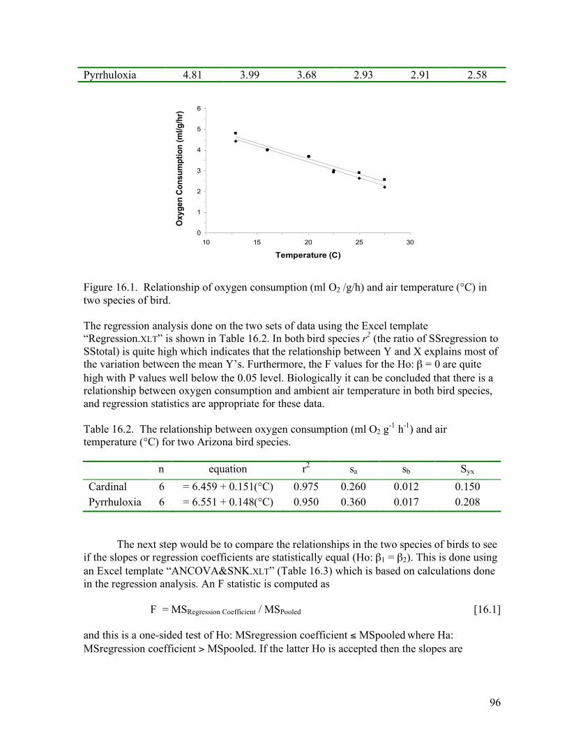
In many cases biologists are interested in comparing regression equations of two or more sets of regression data. In these cases, the interest is in whether the sample slopes (b) are estimates of the same or different population slopes (β). If it is concluded that the regression lines are parallel, that is that the slopes are equal, then there is often interest in determining whether the regressions have the same elevation (i.e. same y-intercept, α) and coincide. The test for coincidence (elevation, or same y-intercept) can only be carried out for those lines that have been demonstrated to have no significant statistical difference in slope. In cases where there are only two lines, a t-test can be used to test the difference between slopes, and if the slopes are equal, then another t-test can be used to determine if the difference in elevation is significant. However, t-tests cannot be used when there are more than two lines; thus, t-tests are limited in their application and their use is not covered in this course. The procedure, which must be used in comparing more than two lines, is known as an analysis of covariance (ANCOVA). It allows for testing Ho: β1 = β2 = β3…= βk with an alternative hypothesis that the regression lines were not derived from samples estimating populations which all had equal slopes. ANCOVA can also be used to compare only two lines where Ho: β1 = β2 and Ha: β1 ≠ β2. Furthermore, ANCOVA also allows for testing whether the elevations are equal for those regression lines, which are demonstrated to come from populations with equal slopes. The null hypothesis is simply that the elevations are equal (the lines coincide) while the alternative hypothesis is that the elevations are not equal (the lines do not coincide). To illustrate how ANCOVA works, let’s consider the relationship of oxygen consumption to air temperature in two bird species that co-occur in semi-desert areas of the southwest (Table 16.1, Figure 16.1). Inspection of the figure indicates that: a) there appears to be a negative relationship between oxygen consumption and ambient air temperature in both species, and b) the relationships appear very similar for the two species. The first step in the analysis of these data is to test if there is a significant relationship between air temperature and oxygen consumption for each species; in other words test Ho: β = 0. If Ho is accepted for both bird species, then one concludes that there is no relationship between oxygen consumption and air temperature (the Y and X axes) in either of these two species, and regression statistics are inappropriate. The appropriate analysis would then be to use an ANOVA to determine if the mean Y values (e.g. oxygen consumption) came from the same population. If Ho: β = 0 is accepted for one species but not the other then the analysis is complete and it is concluded that there is a relationship between oxygen consumption and air temperature for only one species. Finally if Ho: β = 0 is rejected for both species, then ANCOVA can be applied to determine if the relationships are the same for the two species. Table 16.1. Oxygen consumption (ml O2 g-1 h-1) of the cardinal and pyrrhuloxia at various air temperatures (°C). 12.9 °C 16.0 °C 20.1 °C 22.5 °C 25.0 °C 27.5 °C Cardinal 4.44 4.02 3.68 3.02 2.65 2.21

96

Pyrrhuloxia 4.81 3.99 3.68 2.93 2.91 2.58

0

1

2

3

4

5

6

10 15 20 25 30

Temperature (C)

Oxyg

en

Co

nsu

mp

tio

n (

ml/g

/hr)

Figure 16.1. Relationship of oxygen consumption (ml O2 /g/h) and air temperature (°C) in two species of bird. The regression analysis done on the two sets of data using the Excel template “Regression.XLT” is shown in Table 16.2. In both bird species r2 (the ratio of SSregression to SStotal) is quite high which indicates that the relationship between Y and X explains most of the variation between the mean Y’s. Furthermore, the F values for the Ho: β = 0 are quite high with P values well below the 0.05 level. Biologically it can be concluded that there is a relationship between oxygen consumption and ambient air temperature in both bird species, and regression statistics are appropriate for these data. Table 16.2. The relationship between oxygen consumption (ml O2 g-1 h-1) and air temperature (°C) for two Arizona bird species.

n equation r2 sa sb Syx Cardinal 6 = 6.459 + 0.151(°C) 0.975 0.260 0.012 0.150 Pyrrhuloxia 6 = 6.551 + 0.148(°C) 0.950 0.360 0.017 0.208

The next step would be to compare the relationships in the two species of birds to see if the slopes or regression coefficients are statistically equal (Ho: β1 = β2). This is done using an Excel template “ANCOVA&SNK.XLT” (Table 16.3) which is based on calculations done in the regression analysis. An F statistic is computed as F = MSRegression Coefficient / MSPooled [16.1] and this is a one-sided test of Ho: MSregression coefficient ≤ MSpooled where Ha: MSregression coefficient > MSpooled. If the latter Ho is accepted then the slopes are

97

statistically equal; however, if Ho: MSregression coefficient ≤ MSpooled is rejected then the slopes are considered to be statistically (“significantly”) not equal. The pooled MS can be thought of as the average MS residual of all the lines involved. The regression coefficient MS is the difference between the unexplained variation of an “average” slope (common MS) and the unexplained variation averaged from all the lines involved (pooled MS). It basically expresses the variation resulting form differences between slopes. The closer the slopes parallel one another the smaller the MS regression coefficient becomes, and it increase in value as the slopes diverge from one another. It would generally be expected to be smaller than the average unexplained variation of the individual lines; this leads to the Ho that the regression coefficient MS will be less than the pooled MS.

Calculating ANCOVA Using EXCEL The first step using the Excel template “ANCOVA&SNK.XLT” is to copy all the uncorrected sum of squares that were calculated during each of the regression analyses (Figure 16.2).

Figure 16.2. Uncorrected sum of squares calculated during each regression analysis and transferred to the Excel ANCOVA template. From the uncorrected sum of squares, the template computes the MS pooled by summing the residual SS and df of each of the regressions as shown in Figure 16.3. As always MS is computed by dividing SS by its df. The calculation of the MS regression coefficient requires that the common SS first be computed. Each of the corrected sums of squares (SdX2, SdXd, SdY2) of all the lines are summed and placed in the appropriate column in the row entitled “common”. These sums are then used to compute the common SS in the usual manner. The common df is equal to the pooled df plus k-1, where k is the number of lines involved in the analysis. In this example k = 2 and the common df = 9 (=8+1). The regression coefficient SS is simply the difference between the common SS and the pooled SS, and its df = k-1 where again k is the number of lines involved in the analysis.

The F statistic calculated to test Ho: β1 = β2 using equation 16.1 is displayed in the ANCOVA output adjacent to the heading “Ho: slopes equal”. The P(F[α(1)=0.05,1,8]) is also displayed and for this example is very high, and Ho: MS regression coefficient ≤ MS pooled is accepted which means that Ho: β1 = β2 must also be accepted.

98

Figure 16.3. Corrected sums of squares and ANCOVA tests for equal slopes and elevations from the “ANCOVA&SNK.XLT” template. Because the slopes are equal, the elevations of the two lines may be validly compared. If the were not equal, the ANCOVA template would still generate the test statistic but the test would not be valid. The F statistic is generated for testing Ho: elevations equal is computed as

F = MS Adjusted Means/ MS Common [16.2]

Which again is a one-sided test of Ho: MS adjusted means ≤ MS common where Ha: MS adjusted means > MS common. If the latter Ho is accepted, then the elevations are statistically equal; however, if Ho: MS adjusted means ≤ MS common is rejected then the elevations are considered to be statistically (“significantly”) not equal, in other words they are “significantly different.”

The MS adjusted means corresponds to the average difference in elevations between each of the lines involved in the ANCOVA. The adjusted means SS is computed as the difference between the total SS and the common SS. The df for the adjusted means is k-1 or the number of lines involved less one; this is the same df as for the regression coefficient. The total SS is computed by generating uncorrected sums for all the points of all the lines involved in the analysis; thus, all the data are treated as if there is one line and the regression statistics are generated on this one line. This can be done rather quickly by simply totaling the sums of X, Y and uncorrected sums of squares for each of the regression lines involved and then obtaining the corrected sums of squares.

In the example (Table 16.1) the F statistic for “Ho: elevations equal” is displayed adjacent to the associated probability statement. The P(F[α(1)=0.05,1,9] = 2.25) is clearly above

99

the critical P = 0.05 level. Therefore, Ho: MS adjusted means ≤ MS common must be accepted which also means accepting Ho: elevations equal. The biological conclusions made about the two bird species can be summarized as follows:

• There was a linear relationship between oxygen consumption and ambient air temperature for each of the two bird species.

• The two bird species exhibit the same decrease in oxygen consumption per unit change in ambient air temperature.

• The elevations of the two lines were statistically similar; thus, at the same ambient air temperature both bird species exhibit no significant differences in oxygen consumption.

Given that there are only two lines ANCOVA statistics can be used to a) test another hypothesis, and b) quantify the difference in elevation if the difference is significant. These options are covered below. If there are more than two lines, then multiple comparison tests have to be applied to determine where the differences in slope and elevation lie. One of these test, the Student-Newman-Keuls or SNK test is presented in the next chapter. When only two lines are being compared, ANCOVA calculations can be easily used to test if the variability about the two is similar. An F test statistic is computed by dividing the MS residuals of the two lines; the large MS residual is placed in the numerator and the smaller MS residual in the denominator. The dfs equal df of the numerator MS and df of the denominator MS. This is a two-sided F test with Ho: σyx1 = σyx2. In the example problem, F = MS residual2 / MS residual 1 = (0.174/4) / (0.082/4) = 2.122 [16.3]

with 4 df in the numerator and 4 in the denominator. The P(F[α(2)=0.05,4,4] = 2.122) > 0.05, and therefore Ho: σyx1 = σyx2 is accepted. Thus, there is no difference in variability about the lines relating oxygen consumption to ambient air temperature in the Cardinal and Pyrrhuloxia. If the two lines do not have significantly different slopes but do have significantly different elevations, then the magnitude of the difference in elevations can be determined as the difference between the adjusted means of the two lines. The adjusted mean for a line is computed as Yadj = YL - bc (XL – XT) [16.4] Where Yadj = adjusted mean Y for the line, YL = mean of the Y values for the line, bc = common slope from the ANCOVA table, XL = mean of the X values for the line, and XT = mean of all X values for both lines. The magnitude of the difference in elevations is then computed by subtracting Yadj of one line from the other. This calculation is only meaningful if the elevations are significantly different. This was not the case in the two species example (Table 17.1). However, the adjusted means of each line can be computed to illustrate the calculation. In this example the mean of all the X values for both lines (XT, n=10) and the

100

mean of X values for each line (XL) are the same value. Thus, the adjusted means for each line are simply their respective y-intercepts as shown here Cardinal Yadj = 6.428 – (-0.151) (20.667 – 20.667) = 6.428 Pyrrhuloxia Yadj = 6.581 – (-0.148) (20.667 – 20.667) = 6.581 The difference between the two lines, 0.153, is not significant as shown by acceptance of Ho: elevations are equal. Both the test of variability about the lines and quantifying the difference between lines can be conducted in cases where there are more than two lines. However, this is beyond the scope of this course (and also very tedious!).

101

ANCOVA + SNK Analysis of covariance, like ANOVA, only indicates if there are differences between

slopes or elevations but it does not indicate where the difference lies. For example, Ha’s for three lines may be one of the following: β1 ≠ β2 ≠ β3 or β1 ≠ β2 = β3 or β1 = β2 ≠ β3. However, ANCOVA provides information allowing only for deciding whether the slopes and elevations are equal or not. A second procedure must be used to determine where the difference lies in either slopes or, in cases where slopes are the same, elevations. The procedure used is a multiple comparison test called the Student-Newman-Keuls multiple range tests (SNK) for short. It is very similar to the SNK procedure used to determine where differences lie between multiple means (Chapter 9).

The general form of the SNK test is

q = difference between 2 statistics / “average” SE of two statistics

where the generalized Ho is that the 2 variables come from the same population. The degrees of freedom are p, the number of statistics across which the comparison is being made, and the df of “average” standard error of the two statistics. For example, if two slopes are being compared and they are separated in rank by one other slope, then p = 3. In SNK regression the “average” SE of the two statistics always includes the MS pooled from ANCOVA, so the pooled df is the df used in the SNK tests. As always, if the calculated q value is greater than the critical value, the Ho is rejected. The first step is to rank the statistics (e.g. slopes or elevations) from highest to lowest. Then the q test statistics are calculated by comparing the highest with first the lowest, then the next lowest, etc., until all possible comparisons have been made for the highest statistic. The next highest statistic is the compared to the lowest, the next lowest, etc. For example, if five slopes are ranked such that 5 is highest and 1 lowest, then the order of comparison would be: 5 vs 1 5 vs 2 5 vs 3 5 vs 4 then 4 vs 1 4 vs 2 4 vs 3 then 3 vs 1 3 vs 2 then 2 vs 1 Two additional important procedural rules are as follows. First as in all SNK tests, if no difference is found between two statistics, it is concluded that no difference exists between any statistics enclosed by these two. For example, if five slopes are compared and the calculated q of the comparison 5 vs 1 demands acceptance of Ho: β5 = β1, then it must be also concluded that β4 = β3 = β2. Note that this can happen even though ANCOVA demonstrates that there is a significant difference between slopes (one wouldn’t initiate SNK procedures unless this was the case). This simply reflects the fact that ANCOVA is a more powerful test than is the SNK test. A second important procedural rule deals with regression statistics only. Elevations can only be compared for lines with similar slopes. If the slopes are significantly different, elevations cannot be legitimately compared.

102

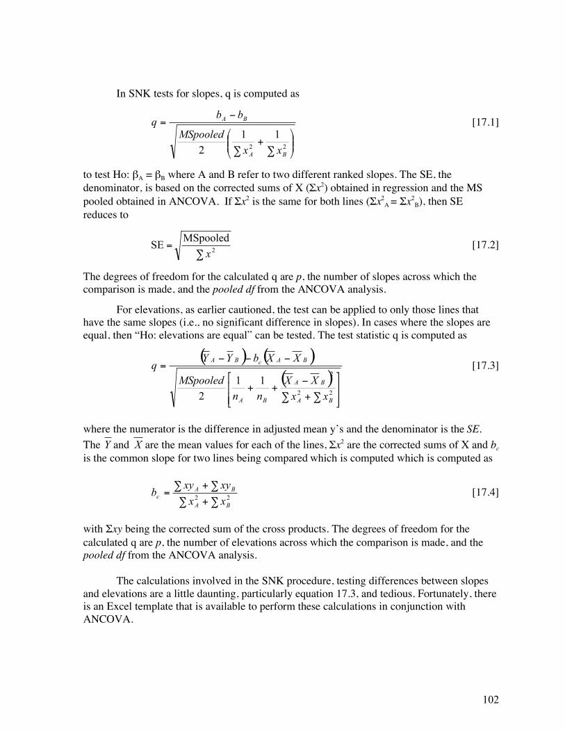
In SNK tests for slopes, q is computed as

!!"

#$$%

&

'+

'

(=

22

11

2BA

BA

xx

MSpooled

bbq [17.1]

to test Ho: βA = βB where A and B refer to two different ranked slopes. The SE, the denominator, is based on the corrected sums of X (Σx2) obtained in regression and the MS pooled obtained in ANCOVA. If Σx2 is the same for both lines (Σx2

A = Σx2B), then SE

reduces to

!

=2

MSpooled SE

x

[17.2]

The degrees of freedom for the calculated q are p, the number of slopes across which the comparison is made, and the pooled df from the ANCOVA analysis.

For elevations, as earlier cautioned, the test can be applied to only those lines that have the same slopes (i.e., no significant difference in slopes). In cases where the slopes are equal, then “Ho: elevations are equal” can be tested. The test statistic q is computed as

( ) ( )

( )!!"

#

$$%

&

' '+

(++

(((=

22

2

11

2BA

BA

BA

BAcBA

xx

XX

nn

MSpooled

XXbYYq [17.3]

where the numerator is the difference in adjusted mean y’s and the denominator is the SE. The Y and X are the mean values for each of the lines, Σx2 are the corrected sums of X and bc is the common slope for two lines being compared which is computed which is computed as

! !+

! !+=

22

BA

BAc

xx

xyxyb [17.4]

with Σxy being the corrected sum of the cross products. The degrees of freedom for the calculated q are p, the number of elevations across which the comparison is made, and the pooled df from the ANCOVA analysis.

The calculations involved in the SNK procedure, testing differences between slopes and elevations are a little daunting, particularly equation 17.3, and tedious. Fortunately, there is an Excel template that is available to perform these calculations in conjunction with ANCOVA.

103

Comparison of Regression Equations Using EXCEL The SNK template is the second worksheet of the EXCEL “ANCOVA&SNK.XLT” template. There are two portions to the SNK analysis 1) comparison of slopes, and 2) comparison of elevations for those lines with equal slopes. Values from the first worksheet, titled ANCOVA, are automatically put into the SNK template. The values are the sample size, slope, Σx2, Σxy, y , and x for each line, for up to ten regression lines from the ANCOVA worksheet. The data are transferred in the order they were entered into the ANCOVA worksheet (Figure 17.1), and as indicted by the instructions, the user has to do a descending sort by slope. It is important that only data be selected before doing the sort. For example, if only four regression lines have been analyzed then it is important to select only the appropriate four rows and not include any additional rows from the data box. Sort can be found under Tools|Sort.

SNK SlopesDo descending sort on slopes (b) in D from A4 to H13 using only rows containing data (no zeros).

ID n b !x2 !xy Mean X Mean Y

1 Sandy,NoTrees 5 .211 125.200 26.378 42.40 40.70 For Elevation SNK

2 Clay,NoTrees 5 .211 250.000 52.650 40.00 40.16 • copy data for lines with same slopes

3 Clay,Trees 5 .164 250.000 41.100 35.00 39.80 • put in blue box in next worksheet

4 Sandy,Trees 5 .088 250.000 22.050 35.00 39.56

5 0 0

6 0 07 0 0

8 0 0

9 0 0

10 0 0 Figure 17.1. Hypothetical data after being sorted by decreasing slope in the “SNK Slopes” worksheet of the ANCOVA & SNK template. After sorting, the q values are calculated appropriately and the analysis is complete. The critical q value is the P=0.05 value and is imported from the 4th worksheet in the ANCOVA&SNK.XLT template. The statistical decision of acceptance or rejection of the null hypothesis is obtained by simply comparing the calculated q to the critical value. If the calculated value is greater than the critical value, then the probability that sample A and B come from the same population is less than 0.05. Thus, the Ho: slopes are equal is rejected. Conversely, a calculated q lower than critical q results in a probability greater than 0.05 that the two samples come from the same population and the Ha: slopes are unequal is accepted. If more than two slopes are found to be equal, then the SNK for comparison of elevations can be completed. The sorted regression data is then copied from the “SNK Slopes” worksheet to the “SNK Elevations” worksheet (Figure 17.2) where it is then sorted by descending mean Y.

The q values for the elevations are then calculated according to equation 17.3, and compared against the critical q values (from the 4th worksheet). The same rules apply for interpreting SNK elevations as applied for SNK slopes; if the calculated q is greater than the

104

critical q then P will be less than 0.05 and the elevations are considered significantly different.

SNK ElevationsDo descending sort on mean Y in Col I from A4 to H13 using only data rows containing data.

ID n b !x2 !xy Mean X Mean Y

1 Sandy,NoTrees 5 .211 125.200 26.378 42.40 40.70

2 Clay,NoTrees 5 .211 250.000 52.650 40.00 40.16

3 Clay,Trees 5 .164 250.000 41.100 35.00 39.80

4 Sandy,Trees 5 .088 250.000 22.050 35.00 39.56

5 Figure 17.2. Hypothetical data after being copied from the “SNK Slopes” worksheet into the “SNK Elevations” and then sorted by descending mean Y.

Example Problem (Problem 17.1)

I. STATISTICAL STEPS A. Statement of Ho and Ha

1. Ho: β = 0 for relationship of cholesterol and age in both sexes with and without drug (4 regressions)

2. Assuming that β ≠ 0 for all lines test: Ho: β women, no drugs = β women, drug = β men, no drug = β men, drug

3. Ho: elevations equal for those lines with equal slopes

B. Statistical test Generate regression statistics on all 4 lines; use ANCOVA to compare the 4 lines, SNK to find out where the differences lie.

C. Computation of test statistics

1. All four regressions of cholesterol and age were found to be significant P < 0.05, and the uncorrected sum of squares is then copied from each regression worksheet into the “ANCOVA&SNK” template.

2. From the “ANCOVA&SNK” template, you find that the null hypothesis of slopes

being equal is accepted because F 3,42 = 0.358 and P = 0.784.

105

3. Because slopes are equal, you check to see if elevations are equal. You reject the null

of elevations being equal because F 3,45 = 56.355 and P < 0.001. This means that elevations are different and you must turn to the “SNK Elevations” worksheet to determine where differences occur.

4. The q values in the “SNK Elevations” worksheet are all larger than critical q values, therefore all of the elevations are significantly different (P < 0.05) with Men, no drug > Women, no drug > Men, drug > Women, drug.

D. Determine of the P of the test statistic 1. Ho: βs = 0 P < 0.05 for all 4 groups 2. Ho: βs equal F[α(1)=0.05, 3, 42] = 0.358, P > 0.05 3. Ho: elevations equal F[α(1)=0.05, 3, 45] = 56.36, P < 0.05

E. Statistical Inference

1. There is a relationship between cholesterol and age in both sexes, with and without drugs.

2. Slopes, change in cholesterol at any fixed age, are the same in both sexes, with and without drugs.

3. Elevations, amount of cholesterol at any fixed age, are higher in men than in women and the drug significantly reduces the elevation in either sex.

106

II. BIOLOGICAL INTERPRETATION

Methods

Regression equations were calculated by the method of least squares for the relationships of blood cholesterol to age in men and women with and without drug therapy. If there were significant regressions between age and blood cholesterol levels for these groups (α = 0.05), differences between slopes and elevations of the regression equations were tested using analysis of covariance and Student-Newman-Keuls post tests (α = 0.05). Elevations of the regression lines were compared only if the slopes were not significantly different; differences in elevation are presented at the mean age for each sample.

Results

For both men and women, with and without drug therapy, there was a significant relationship between age and blood cholesterol levels (F = 8.02 – 345.5, P = 0.02 - < 0.001 for all regressions), and all regressions had the same slope (Table 1). Therapy with drug ZZZ significantly reduced the elevation of the relationship of blood cholesterol to age in both men and women (Table 1). Drug therapy reduced cholesterol levels slightly more in women (55%) than in men (44%). With or without drug therapy, men had significantly higher cholesterol levels at any age than did women (Fig. 1). Neither gender nor drug therapy affected the increase in blood cholesterol with increasing age (i.e., slopes). Table 1. Relationship of blood cholesterol (mg/dL) to age (Yr, years) in men and women with and without therapy using drug ZZZ. Group n Equation syx sb sa R2

Drug Men 10 = -32.9 + 3.0 (Yr) 7.1 0.2 8.3 0.98 Women 10 = -45.1 + 2.2 (Yr) 16.6 0.4 26.6 0.78 Control Men 19 = 102.0 + 2.5 (Yr) 39.9 0.5 26.1 0.56 Women 11 = 35.8 + 3.2 (Yr) 48.9 1.1 62.5 0.47

Slopes, F = 0.363, P > 0.05

Elevations, F = 55.986, P < 0.01

107

0

50

100

150

200

250

300

350

400

0 20 40 60 80 100

Age (years)

Blo

od

Ch

ole

ste

rol (m

g/1

00m

l)

Figure 1. Relationship of blood cholesterol to age in men (squares) and women (circles) with (filled symbols) and without (open symbols) therapy using drug ZZZ.

108

Problem Set – ANCOVA Determine if the relationship between oxygen consumption (ml O2 g-1 h-1) and ambient air temperature (°C) is different for the two bird species in questions 16.1 to 16.3. 16.1) Following are the same data given in the sample problem.

12.9 °C 16.0 °C 20.1 °C 22.5 °C 25.0 °C 27.5 °C Cardinal 4.44 4.02 3.68 3.02 2.65 2.21 Pyrrhuloxia 4.81 3.99 3.68 2.93 2.91 2.58

16.2) The following data are derived from those given in 17.1 except the oxygen

consumption values for the cardinal have been decreased by 10%. What do expect to happen to the analysis?

12.9 °C 16.0 °C 20.1 °C 22.5 °C 25.0 °C 27.5 °C Cardinal 4.00 3.64 3.31 2.57 2.38 1.98 Pyrrhuloxia 4.81 3.99 3.68 2.93 2.91 2.58

16.3) The following data are derived from those given in 17.1 except the oxygen

consumption values for the cardinal have been decreased by a particular percentage which increases with increasing temperature (i.e. 5% at 16°, 10% at 20.1°, etc.). What do expect to happen to the analysis? 12.9 °C 16.0 °C 20.1 °C 22.5 °C 25.0 °C 27.5 °C Cardinal 4.00 3.82 3.31 2.75 2.12 1.66 Pyrrhuloxia 4.81 3.99 3.68 2.93 2.91 2.58

16.4) Determine if the relationship between oxygen consumption (liters min-1) and power

outputs (Watts) on a bicycle ergometer varies between an athlete and nonathlete. 0 50 100 150 200 250 Athlete 0.3 0.9 1.5 2.2 2.9 3.5 Nonathlete 0.3 1.4 2.4 2.9

16.5) Physical fitness test scores of three groups of individuals whose daily exercise regimes

varied. Age Inactive Moderate Active 43 4.36 2.68 3.69 44 5.50 3.94 5.13 42 6.64 5.20 6.57

16.6) Investigators wished to know if beer affected the respiratory exchange ratio (RQ) of top athletes at different time intervals during sub-maximal exercise.

Time Beer Water No liquid 15 87.0 84.5 85.75 20 86.0 83.0 84.5 25 85.2 81.75 82.75 30 84.0 80.5 81.0