chapter 14 weighted graphs and applications · pdf file · 2008-08-02interface, the...
TRANSCRIPT
809
CHAPTER 14 Weighted Graphs and Applications Objectives
• To represent weighted edges using adjacency matrices and priority queues (§14.2).
• To model weighted graphs using the WeightedGraph class that extends the AbstractGraph class (§14.3).
• To understand and implement the algorithm for finding a minimum spanning tree (§14.4).
• To define the MST class that extends the Tree class (§14.4).
• To understand and implement the algorithm for finding single-source shortest paths (§14.5).
• To define the ShortestPathTree class that extends the Tree class (§14.5).
• To solve the weighted nine tail problem using the shortest path algorithm (§14.6).
810
14.1 Introduction The preceding chapter introduced the concept of graphs. You learned how to represent edges using edge arrays, edge lists, adjacency matrices, and adjacency lists, and how to model a graph using the Graph interface, the AbstractGraph class, and the UnweightedGraph class. The preceding chapter also introduced two important techniques for traversing graphs: depth-first search and breadth-first search, and applied traversal to solve practical problems. This chapter will introduce weighted graphs. You will learn the algorithm for finding a minimum spanning tree in Section 14.2 and the algorithm for finding shortest paths in Section 14.4. 14.2 Representing Weighted Graphs There are two types of weighted graphs: vertex-weighted graphs and edge-weighted graphs. In a vertex-weighted graph, each vertex is assigned a weight. In an edge-weighted graph, each edge is assigned a weight. Edge-weighted graphs have more applications than vertex-weighted graphs. This chapter considers edge-weighted graphs. Weighted graphs can be represented in the same way as unweighted graphs except that you have to represent the weights on the edges. Like unweighted graphs, the vertices in weighted graphs can be stored in an array. This section introduces three representations for the edges in weighted graphs. <Side Remark: integer weights> For simplicity, we assume that the weights are integers in this chapter. 14.2.1 Representing Weighted Edges: Edge Array
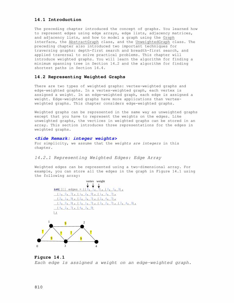
Weighted edges can be represented using a two-dimensional array. For example, you can store all the edges in the graph in Figure 14.1 using the following array:
int[][] edges = {{0, 1, 7}, {0, 3, 9},
{1, 0, 7}, {1, 2, 9}, {1, 3, 7},
{2, 1, 9}, {2, 3, 7}, {2, 4, 7},
{3, 0, 9}, {3, 1, 7}, {3, 2, 7}, {3, 4, 9},
{4, 2, 7}, {4, 3, 9}
};
7 7
9
9 7
9
7
0
1 2
3 4 Figure 14.1 Each edge is assigned a weight on an edge-weighted graph.
vertex weight

811
NOTE
<Side Remark: integer weights> For simplicity, we assume that the weights are integers. Weights can be of any type. In that case, you may use a two-dimensional array of the Object type as follows:
Object[][] edges = {
{new Ineger(0), new Ineger(1), new SomeTypeForWeight(7)},
{new Ineger(0), new Ineger(3), new SomeTypeForWeight(9)},
...
};
14.2.2 Weighted Adjacency Matrices
Assume that the graph has n vertices. You can use a two-dimensional n×n matrix, say weights, to represent the weights on edges. weights[i][j] represents the weight on edge (i, j). If vertices i and j are not connected, weights[i][j] is null. For example, the weights in the graph in Figure 14.1 can be represented using an adjacency matrix as follows:
Integer[][] adjacencyMatrix = {
{null, 7, null, 9, null },
{7, null, 9, 7, null },
{0, 9, null, 7, 7},
{9, 7, 7, null, 9},
{null, null, 7, 9, null}
};
14.2.3 Priority Adjacency Lists
Another way to represent the edges is to define edges as objects. The AbstractGraph.Edge class was defined to represent edges in unweighted graphs. For weighted edges, we define the WeightedEdge class as shown in Listing 14.1.
Listing 14.1 WeightedEdge.java
***PD: Please add line numbers in the following code*** ***Layout: Please layout exactly. Don’t skip the space. This is true for all source code in the book. Thanks, AU. <Side Remark line 3: edge weight> <Side Remark line 6: constructor> <Side Remark line 12: compare edges>
public class WeightedEdge extends AbstractGraph.Edge
implements Comparable<WeightedEdge> {
public int weight; // The weight on edge (u, v)
/** Create a weighted edge on (u, v) */
public WeightedEdge(int u, int v, int weight) {
super(u, v);
this.weight = weight;
}

812
/** Compare two edges on weights */
public int compareTo(WeightedEdge edge) {
if (weight > edge.weight) {
return 1;
}
else if (weight == edge.weight) {
return 0;
}
else {
return -1;
}
}
} AbstractGraph.Edge is an inner class defined in the AbstractGraph class. It represents an edge from vertex u to v. WeightedEdge extends AbstractGraph.Edge with a new property weight. To create an Edge object, use new Edge(i, j, w), where w is the weight on edge (i, j). Often it is desirable to store a vertex’s adjacent edges in a priority queue so that you can remove the edges in increasing order of their weights. For this reason, the Edge class implements the Comparable interface. For unweighted graphs, we use adjacency lists to represent edges. For weighted graphs, we still use adjacency lists, but the lists are priority queues. For example, the adjacency lists for the vertices in the graph in Figure 14.l can be represented as follows:
java.util.PriorityQueue<Edge>[5] queues =
new java.util.PriorityQueue<Edge>();
queues[0]
queues[1]
queues[2]
queues[3]
queues[4]
WeightedEdge(0, 1, 7) WeightedEdge(0, 3, 9)
WeightedEdge(1, 0, 7) WeightedEdge(1, 3, 7) WeightedEdge(1, 2, 9)
WeightedEdge(2, 3, 7) WeightedEdge(2, 4, 7) WeightedEdge(2, 1, 9)
WeightedEdge(3, 1, 7) WeightedEdge(3, 2, 7) WeightedEdge(3, 0, 9) WeightedEdge(3, 4, 9)
WeightedEdge(4, 2, 7) WeightedEdge(4, 3, 9)
queues[i] stores all edges adjacent to vertex i. 14.3 The WeightedGraph Class The preceding chapter designed the Graph interface, the AbstratGraph class, and the UnweightedGraph class for modeling graphs. Following this pattern, we design WeightedGraph as a subclass of AbstractGraph, as shown in Figure 14.2. <PD: UML Class Diagram>

813
«interface» Graph
AbstractGraph
WeightedGraph
-queues: java.util.PriorityQueue<WeightedEdge>[]
+WeightedGraph(edges: int[][], vertices: Object[])
+WeightedGraph(edges: List<WeightedEdge>, vertices: List)
+WeightedGraph(edges: int[][], numberOfVertices: int)
+WeightedGraph(edges: List<WeightedEdge>, numberOfVertices: int)
+printWeightedEdges(): void +getMinimumSpanningTree(): MST +getMinimumSpanningTree(v: int): MST +getShortestPath(v: int): ShortestPathTree
queues[i] is a priority queue that contains all the edges adjacent to vertex i.
Constructs a weighted graph with specified edges and the number of vertices in arrays.
Constructs a weighted graph with specified edges and the number of vertices.
Constructs a weighted graph with specified edges in an array and the number of vertices.
Constructs a weighted graph with specified edges in a list and the number of vertices.
Displays all edges and weights. Returns a minimum spanning tree starting from vertex 0. Returns a minimum spanning tree starting from vertex v. Returns all single source shortest paths.
Figure 14.2 WeightedGraph extends AbstractGraph. WeightedGraph simply extends AbstractGraph with four constructors for creating concrete weighted Graph instances. WeightedGraph inherits all methods from AbstractGraph and it also introduces the new methods for obtaining minimum spanning trees and for finding single source all shortest paths. Minimum spanning trees and shortest paths will be introduced in §14.3 and §14.4, respectively. Listing 14.2 implements WeightedGraph. Priority adjacency lists (line 8) are used internally to store adjacent edges for a vertex. When a WeightedGraph is constructed, its priority adjacency lists are created (lines 14, 21, 28, and 36). The methods getMinimumSpanningTree() (lines 81-164) and getShortestPaths() (lines 167-246) will be introduced in the upcoming sections.
Listing 14.2 WeightedGraph.java
***PD: Please add line numbers in the following code*** ***Layout: Please layout exactly. Don’t skip the space. This is true for all source code in the book. Thanks, AU. <Side Remark line 8: priority queue> <Side Remark line 12: constructor> <Side Remark line 13: superclass constructor> <Side Remark line 14: create priority queues> <Side Remark line 19: constructor> <Side Remark line 26: constructor> <Side Remark line 33: constructor> <Side Remark line 40: create priority queues> <Side Remark line 43: create queues> <Side Remark line 51: fill queues> <Side Remark line 56: create priority queues>

814
<Side Remark line 60: create queues> <Side Remark line 64: fill queues> <Side Remark line 69: print edges> <Side Remark line 81: minimum spanning tree> <Side Remark line 82: start from vertex 0> <Side Remark line 86: minimum spanning tree> <Side Remark line 99: deep clone> <Side Remark line 87: vertices in tree> <Side Remark line 89: add to tree> <Side Remark line 91: number of vertices> <Side Remark line 92: parent array> <Side Remark line 95: initialize parent> <Side Remark line 96: total weight> <Side Remark line 99: a copy of queues> <Side Remark line 102: more vertices?> <Side Remark line 107: every u in tree> <Side Remark line 112: remove visited vertex> <Side Remark line 115: queues[u] is empty> <Side Remark line 120: smallest edge to u> <Side Remark line 123: update smallestWeight> <Side Remark line 129: add to tree> <Side Remark line 130: update totalWeight> <Side Remark line 137: clone queue> <Side Remark line 145: clone every element> <Side Remark line 153: MST inner class> <Side Remark line 154: total weight in tree> <Side Remark line 169: vertices found> <Side Remark line 171: add source> <Side Remark line 174: number of vertices> <Side Remark line 177: parent array> <Side Remark line 178: parent of root> <Side Remark line 181: costs array> <Side Remark line 185: source cost> <Side Remark line 188: a copy of queues> <Side Remark line 191: more vertices left?> <Side Remark line 192: determine one> <Side Remark line 197: remove visited vertex> <Side Remark line 202: queues[u] is empty> <Side Remark line 207: smallest edge to u> <Side Remark line 208: update smallestCost> <Side Remark line 210: v now found> <Side Remark line 214: add to T> <Side Remark line 219: create a path> <Side Remark line 224: costs> <Side Remark line 227: constructor> <Side Remark line 233: get cost> <Side Remark line 239: print all paths>

815
import java.util.*;
public class WeightedGraph extends AbstractGraph {
// Priority adjacency lists
private PriorityQueue<WeightedEdge>[] queues;
/** Construct a WeightedGraph with speficied edges and vertice in
* arrays */
public WeightedGraph(int[][] edges, Object[] vertices) {
super(edges, vertices);
createQueues(edges, vertices.length);
}
/** Construct a WeightedGraph with speficied edges in
* an array and the number of vertices */
public WeightedGraph(int[][] edges, int numberOfVertices) {
super(edges, numberOfVertices);
createQueues(edges, numberOfVertices);
}
/** Construct a WeightedGraph with speficied edges and vertice in
* lists */
public WeightedGraph(List<WeightedEdge> edges, List vertices) {
super((List)edges, vertices);
createQueues(edges, vertices.size());
}
/** Construct a WeightedGraph with speficied edges in
* a list and the number of vertices */
public WeightedGraph(List<WeightedEdge> edges,
int numberOfVertices) {
super((List)edges, numberOfVertices);
createQueues(edges, numberOfVertices);
}
/** Create priority adjacency lists from edge arrays */
public void createQueues(int[][] edges, int numberOfVertices) {
queues = new java.util.PriorityQueue[numberOfVertices];
for (int i = 0; i < queues.length; i++) {
queues[i] = new java.util.PriorityQueue(); // Create a queue
}
for (int i = 0; i < edges.length; i++) {
int u = edges[i][0];
int v = edges[i][1];
int weight = edges[i][2];
// Insert an edge into the queue
queues[u].offer(new WeightedEdge(u, v, weight));
}
}
/** Create priority adjacency lists from edge lists */
public void createQueues(List<WeightedEdge> edges,
int numberOfVertices) {
queues = new PriorityQueue[numberOfVertices];
for (int i = 0; i < queues.length; i++) {

816
queues[i] = new java.util.PriorityQueue(); // Create a queue
}
for (WeightedEdge edge: edges) {
queues[edge.u].offer(edge); // Insert an edge into the queue
}
}
/** Display edges with weights */
public void printWeightedEdges() {
for (int i = 0; i < queues.length; i++) {
System.out.print("Vertex " + i + ": ");
for (WeightedEdge edge : queues[i]) {
System.out.print("(" + edge.u +
", " + edge.v + ", " + edge.weight + ") ");
}
System.out.println();
}
}
/** Get a minimum spanning tree rooted at vertex 0 */
public MST getMinimumSpanningTree() {
return getMinimumSpanningTree(0);
}
/** Get a minimum spanning tree rooted at a specified vertex */
public MST getMinimumSpanningTree(int startingVertex) {
Set<Integer> T = new HashSet<Integer>();
// T initially contains the startingVertex;
T.add(startingVertex);
int numberOfVertices = vertices.length; // Number of vertices
int[] parent = new int[numberOfVertices]; // Parent of a vertex
// Initially set the parent of all vertices to -1
for (int i = 0; i < parent.length; i++)
parent[i] = -1;
int totalWeight = 0; // Total weight of the tree thus far
// Clone the priority queue, so to keep the original queue intact
PriorityQueue<WeightedEdge>[] queues = deepClone(this.queues);
// All vertices are found?
while (T.size() < numberOfVertices) {
// Search for the vertex with the smallest edge adjacent to
// a vertex in T
int v = -1;
double smallestWeight = Double.MAX_VALUE;
for (int u : T) {
while (!queues[u].isEmpty() &&
T.contains(queues[u].peek().v)) {
// Remove the edge from queues[u] if the adjacent
// vertex of u is already in T
queues[u].remove();
}
if (queues[u].isEmpty()) {

817
continue; // Consider the next vertex in T
}
// Current smallest weight on an edge adjacent to u
WeightedEdge edge = queues[u].peek();
if (edge.weight < smallestWeight) {
v = edge.v;
smallestWeight = edge.weight;
// If v is added to the tree, u will be its parent
parent[v] = u;
}
} // End of for
T.add(v); // Add a new vertex to the tree
totalWeight += smallestWeight;
} // End of while
return new MST(startingVertex, parent, totalWeight);
}
/** Clone an array of queues */
private PriorityQueue<WeightedEdge>[] deepClone(
PriorityQueue<WeightedEdge>[] queues) {
PriorityQueue<WeightedEdge> [] copiedQueues =
new PriorityQueue[queues.length];
for (int i = 0; i < queues.length; i++) {
copiedQueues[i] = new PriorityQueue<WeightedEdge>();
for (WeightedEdge e : queues[i]) {
copiedQueues[i].add(e);
}
}
return copiedQueues;
}
/** MST is an inner class in WeightedGraph */
public class MST extends Tree {
private int totalWeight; // Total weight of all edges in the tree
public MST(int root, int[] parent, int totalWeight) {
super(root, parent);
this.totalWeight = totalWeight;
}
public int getTotalWeight() {
return totalWeight;
}
}
/** Find single source shortest paths */
public ShortestPathTree getShortestPath(int sourceVertex) {
// T stores the vertices whose path found so far
Set<Integer> T = new HashSet<Integer>();
// T initially contains the sourceVertex;
T.add(sourceVertex);

818
// vertices is defined in AbstractGraph
int numberOfVertices = vertices.length;
// parent[v] stores the previous vertex of v in the path
int[] parent = new int[numberOfVertices];
parent[sourceVertex] = -1; // The parent of source is set to -1
// costs[v] stores the cost of the path from v to the source
int[] costs = new int[numberOfVertices];
for (int i = 0; i < costs.length; i++) {
costs[i] = Integer.MAX_VALUE; // Initial cost set to infinity
}
costs[sourceVertex] = 0; // Cost of source is 0
// Get a copy of queues
PriorityQueue<WeightedEdge> [] queues = deepClone(this.queues);
// Expand verticesFound
while (T.size() < numberOfVertices) {
int v = -1; // Vertex to be determined
int smallestCost = Integer.MAX_VALUE; // Set to infinity
for (int u : T) {
while (!queues[u].isEmpty() &&
T.contains(queues[u].peek().v)) {
queues[u].remove(); // Remove the vertex in verticesFound
}
if (queues[u].isEmpty()) {
// All vertices adjacent to u are in verticesFound
continue;
}
WeightedEdge e = queues[u].peek();
if (costs[u] + e.weight < smallestCost) {
v = e.v;
smallestCost = costs[u] + e.weight;
// If v is added to the tree, u will be its parent
parent[v] = u;
}
} // End of for
T.add(v); // Add a new vertex to the set
costs[v] = smallestCost;
} // End of while
// Create a ShortestPathTree
return new ShortestPathTree(sourceVertex, parent, costs);
}
/** ShortestPathTree is an inner class in WeightedGraph */
public class ShortestPathTree extends Tree {
private int[] costs; // costs[v] is the cost from v to source
/** Construct a path */
public ShortestPathTree(int source, int[] parent, int[] costs) {

819
super(source, parent);
this.costs = costs;
}
/** Return the cost for a path from the root to vertex v */
public int getCost(int v) {
return costs[v];
}
/** Print paths from all vertices to the source */
public void printAllPaths() {
System.out.println("All shortest paths from " +
vertices[getRoot()] + " are:");
for (int i = 0; i < costs.length; i++) {
printPath(i); // Print a path from i to the source
System.out.println("(cost: " + costs[i] + ")"); // Path cost
}
}
}
} When you construct a WeightedGraph, its superclass’s constructor is invoked (lines 11, 18, 23, 33) to initialize the properties vertices and neighbors in AbstrctGraph. Additionally, priority queues are created for instances of WeightedGraph. Listing 14.3 gives a test program that creates a graph for the one in Figure 27.1 and another graph for the one in Figure 14.1.
Listing 14.3 TestWeightedGraph.java
***PD: Please add line numbers in the following code*** ***Layout: Please layout exactly. Don’t skip the space. This is true for all source code in the book. Thanks, AU. <Side Remark line 3: vertices> <Side Remark line 7: edges> <Side Remark line 25: create graph> <Side Remark line 27: print edges> <Side Remark line 29: edges> <Side Remark line 36: create graph> <Side Remark line 38: print edges>
public class TestWeightedGraph {
public static void main(String[] args) {
String[] vertices = {"Seattle", "San Francisco", "Los Angeles",
"Denver", "Kansas City", "Chicago", "Boston", "New York",
"Atlanta", "Miami", "Dallas", "Houston"};
int[][] edges = {
{0, 1, 807}, {0, 3, 1331}, {0, 5, 2097},
{1, 0, 807}, {1, 2, 381}, {1, 3, 1267},
{2, 1, 381}, {2, 3, 1015}, {2, 4, 1663}, {2, 10, 1435},
{3, 0, 1331}, {3, 2, 1015}, {3, 4, 599}, {3, 5, 1003},
{4, 2, 1663}, {4, 3, 599}, {4, 5, 533}, {4, 7, 1260},
{4, 8, 864}, {4, 10, 496},
{5, 0, 2097}, {5, 3, 1003}, {5, 4, 533},
{5, 6, 983}, {5, 7, 787},

820
{6, 5, 983}, {6, 7, 214},
{7, 4, 1260}, {7, 5, 787},
{8, 4, 864}, {8, 7, 888}, {8, 9, 661},
{8, 10, 781}, {8, 11, 810},
{9, 8, 661}, {9, 11, 1187},
{10, 2, 1435}, {10, 4, 496}, {10, 8, 781}, {10, 11, 239},
{11, 8, 810}, {11, 9, 1187}, {11, 10, 239}
};
WeightedGraph graph1 = new WeightedGraph(edges, vertices);
System.out.println("The edges for graph1:");
graph1.printWeightedEdges();
edges = new int[][]{
{0, 1, 7}, {0, 3, 9},
{1, 0, 7}, {1, 2, 9}, {1, 3, 7},
{2, 1, 9}, {2, 3, 7}, {2, 4, 7},
{3, 0, 9}, {3, 1, 7}, {3, 2, 7}, {3, 4, 9},
{4, 2, 7}, {4, 3, 9}
};
WeightedGraph graph2 = new WeightedGraph(edges, 5);
System.out.println("The edges for graph2:");
graph2.printWeightedEdges();
}
}
<Output> The edges for graph1:
Vertex 0: (0, 1, 807) (0, 3, 1331) (0, 5, 2097)
Vertex 1: (1, 2, 381) (1, 0, 807) (1, 3, 1267)
Vertex 2: (2, 1, 381) (2, 3, 1015) (2, 4, 1663) (2, 10, 1435)
Vertex 3: (3, 4, 599) (3, 5, 1003) (3, 2, 1015) (3, 0, 1331)
Vertex 4: (4, 10, 496) (4, 8, 864) (4, 5, 533) (4, 2, 1663)
(4, 7, 1260) (4, 3, 599)
Vertex 5: (5, 4, 533) (5, 7, 787) (5, 3, 1003) (5, 0, 2097)
(5, 6, 983)
Vertex 6: (6, 7, 214) (6, 5, 983)
Vertex 7: (7, 5, 787) (7, 4, 1260)
Vertex 8: (8, 9, 661) (8, 10, 781) (8, 4, 864) (8, 7, 888)
(8, 11, 810)
Vertex 9: (9, 8, 661) (9, 11, 1187)
Vertex 10: (10, 11, 239) (10, 4, 496) (10, 8, 781) (10, 2, 1435)
Vertex 11: (11, 10, 239) (11, 9, 1187) (11, 8, 810)
The edges for graph2:
Vertex 0: (0, 1, 7) (0, 3, 9)
Vertex 1: (1, 0, 7) (1, 2, 9) (1, 3, 7)
Vertex 2: (2, 3, 7) (2, 1, 9) (2, 4, 7)
Vertex 3: (3, 1, 7) (3, 0, 9) (3, 2, 7) (3, 4, 9)
Vertex 4: (4, 2, 7) (4, 3, 9)
<End Output> The program creates graph1 for the graph in Figure 13.1 in lines 3-25. The vertices for graph1 are defined in lines 5-7. The edges for graph1 are defined in 7-23. The edges are represented using a two-dimensional array. For each row i in the array, edges[i][0] and edges[i][1]

821
indicate that there is an edge from vertex edges[i][0] to vertex edges[i][1] and the weight for the edge is edges[i][2]. For example, the first row {0, 1, 807} represents the edge from vertex 0 (edges[0][0]) to vertex 1 (edges[0][1]) with weight 807 (edges[0][2]). The row {0, 5, 2097} represents the edge from vertex 0 (edges[1][0]) to vertex 5 (edges[1][1]) with weight 2097 (edges[1][2]). Line 27 invokes the printWeightedEdges() method on graph1 to display all edges in graph1. The program creates the edges for graph2 for the graph in Figure 14.1 in lines 29-36. Line 38 invokes the printWeightedEdges() method on graph2 to display all edges in graph2.
NOTE: <Side Remark: Traversing priority queue>
The adjacent edges for each vertex are stored in a priority queue. When you remove an edge from the queue, the one with the smallest weight is always removed. However, if you traverse the edges in the queue, the edges are not necessarily in increasing order of weights.
14.4 Minimum Spanning Trees A graph may have many spanning trees. Suppose that the edges are weighted. A minimum spanning tree is a spanning tree with the minimum total weights. For example, the trees in Figures 14.3(b), 14.3(c), 14.3(d) are spanning trees for the graph in Figure 14.3(a). The trees in Figures 14.3(c) and 14.3(d) are minimum spanning trees.
5 6
10
5
8
7
7
12
7
10
8
8
5
5
10
7 7 8
(a) (b)
5
5
6 7
7 8
5
5
6
7 7 8
(c) (d)

822
Figure 14.3 The tree in (c) and (d) are minimum spanning trees of the graph in (a). The problem of finding a minimum spanning tree has many applications. Consider a company with branches in many cities. The company wants to lease telephone lines to connect all branches together. The phone company charges different amounts of money to connect different pairs of cities. There are many ways to connect all branches together. The cheapest way is to find a spanning tree with the minimum total rates. 14.4.1 Minimum Spanning Tree Algorithms
<Side Remark: Prim’s algorithm> How do you find a minimum spanning tree? There are several well-known algorithms for finding a minimum spanning tree. This section introduced Prim’s algorithm. Prim’s algorithm starts with a spanning tree T that contains an arbitrary vertex. The algorithm expands the tree by adding a vertex with the smallest edge incident to a vertex already in the tree. The algorithm can be described in Listing 14.4.
Listing 14.4 Prim’s Minimum Spanning Tree Algorithm
***PD: Please add line numbers in the following code*** ***Layout: Please layout exactly. Don’t skip the space. This is true for all source code in the book. Thanks, AU. <Side Remark line 3: add initial vertex> <Side Remark line 5: more vertices?> <Side Remark line 6: find a vertex> <Side Remark line 7: add to tree>
minimumSpanningTree() {
Let V denote the set of vertices in the graph;
Let T be a set for the vertices in the spanning tree;
Initially, add the starting vertex to T;
while (size of T < n) {
find u in T and v in V – T with the smallest weight
on the edge (u, v), as shown in Figure 14.4;
add v to T;
}
}
u
v
T
V - TVertices already in the spanning tree
Vertices not currently in the spanning tree
Figure 14.4

823
Find a vertex u in T that connects a vertex v in V – T with the smallest weight. The algorithm starts by adding the starting vertex into T. It then continuously adds a vertex (say v) from V – T into T. v is the vertex that is adjacent to a vertex in T with the smallest weight on the edge. For example, there are five edges connecting vertices in T and V – T, as shown in Figure 14.4, (u, v) is the one with the smallest weight. <Side Remark: example> Consider the graph in Figure 14.3(a). The algorithm adds the vertices to T in this order:
• Add vertex 0 to T. • Add vertex 5 to T, since Edge(5, 1, 5) has the smallest weight,
as shown in Figure 14.5(a). • Add vertex 1 to T, since Edge(1, 0, 6) has the smallest weight
among all edges adjacent to the vertices in T, as shown in Figure 14.5(b).
• Add vertex 6 to T, since Edge(6, 1, 7) has the smallest weight among all edges adjacent to the vertices in T, as shown in Figure 14.5(c).
• Add vertex 2 to T, since Edge(2, 6, 5) has the smallest weight among all edges adjacent to the vertices in T, as shown in Figure 14.5(d).
• Add vertex 4 to T, since Edge(4, 6, 7) has the smallest weight among all edges adjacent to the vertices in T, as shown in Figure 14.5(e).
• Add vertex 3 to T, since Edge(3, 2, 8) has the smallest weight among all edges adjacent to the vertices in T, as shown in Figure 14.5(f).
6
5 4
3
2
0
5 6
10
5
8
7
7
12
7
10
8
8
1
6
5 4
3
2
0
56
10
5
8
7
7
12
7
10
8
8
1
(a) (b)
6
5 4
3
2
0
5 6
10
5
8
7
7
12
7
10
8
8
1
6
5 4
3
2
0
56
10
5
8
7
7
12
7
10
8
8
1
(c) (d)

824
6
5 4
3
2
0
5 6
10
5
8
7
7
12
7
10
8
8
1
6
5 4
3
2
0
56
10
5
8
7
7
12
7
10
8
8
1
(e) (f) Figure 14.5 The adjacent vertices with the smallest weight are added to T successively.
NOTE: <Side Remark: unique tree?>
A minimum spanning tree is not unique. For example, both 14.3(c) and 14.3(d) are minimum spanning trees for the graph in Figure 14.1(a). However, if the weights are distinct, the graph has a unique minimum spanning tree.
NOTE:
<Side Remark: connected and undirected> Assume that the graph is connected and undirected. If a graph is not connected or directed, the program may not work. You may modify the program to find a spanning forest for any undirected graph. See Exercise 14.??.
14.4.2 Implementation of the MST Algorithm
<Side Remark: getMinimumSpanningTree()> The getMinimumSpanningTree(int v) method is defined in the WeightedGraph class. It returns an instance of the MST class, as shown in Figure 14.2. The MST class is defined as an inner class in the WeightedGraph class, which extends the Tree class, as shown in Figure 14.6. The Tree class was shown in Figure 27.9. The MST class was implemented in lines 153-164 in Listing 14.2.

825
AbstractGraph.Tree
WeightedGraph.MST
-totalWeight: int
+MST(root: int, parent: int[], totalWeight: int)
+getTotalWeight(): int
Total weight of the tree.
Constructs a MST with the specified root, parent array, and total weight for the tree.
Returns the totalWeight of the tree.
Figure 14.6 The MST class extends the Tree class. The getMinimumSpanningTree method was implemented in lines 81-134 in Listing 14.2. The getMinimumSpanningTree(int startingVertex) method first adds startingVertex to T (line 89). T is a set that stores the vertices currently in the spanning tree (line 87). vertices is defined as a protected data field in the AbstractGraph class, which is an array that stores all vertices in the graph. vertices.length returns the number of the vertices in the graph (line 91). A vertex is added to T if it is adjacent to one of the vertices in T with the smallest weight (line 52). Such vertex is found using the following procedure:
(1) For each vertex u in T, find its neighbor with the smallest weight to u. All the neighbors of u are stored in queues[u]. queues[u].peek() (line 109) returns the adjacent edge with the smallest weight. If a neighbor is already in T, remove it (line 112). To keep the original queues intact, a copy of the queues are created in line 99. After lines 108-117, queues[u].peek() (line 120) returns the vertex with the smallest weight to u.
(2) Compare all these neighbors and find the one with the smallest weight (lines 121-126).
After a new vertex is added to T (line 129), totalWeight is updated (line 130). Once all vertices are added to T, an instance of MST is created (line 133). The MST class extends the Tree class (line 153). To create an instance of MST, pass root, parent, and totalWeight (lines 133). The data fields root and parent are defined in the Tree class, which is an inner class defined in AbstractGraph. <Side Remark: Prim’s algorithm time complexity> For each vertex, the program constructs a priority queue for its adjacent edges. It takes O(log|V|) time to insert an edge to a priority queue and the same time to remove an edge from the priority queue. So the overall time complexity for the program is |)|log|(| VEO , where |E| denotes the number of edges and |V| denotes the number of vertices. Listing 14.5 gives a test program that displays a minimum spanning tree for the graph in Figure 27.1 and a minimum spanning tree for the graph in Figure 14.1, respectively.
Listing 14.5 TestMinimumSpanningTree.java

826
***PD: Please add line numbers in the following code*** ***Layout: Please layout exactly. Don’t skip the space. This is true for all source code in the book. Thanks, AU. <Side Remark line 1: create vertices> <Side Remark line 5: create edges> <Side Remark line 23: create graph1> <Side Remark line 25: MST for graph1> <Side Remark line 26: total weight> <Side Remark line 27: print tree> <Side Remark line 29: create edges> <Side Remark line 36: create graph2> <Side Remark line 37: MST for graph2> <Side Remark line 38: total weight> <Side Remark line 39: print tree>
public class TestMinimumSpanningTree {
public static void main(String[] args) {
String[] vertices = {"Seattle", "San Francisco", "Los Angeles",
"Denver", "Kansas City", "Chicago", "Boston", "New York",
"Atlanta", "Miami", "Dallas", "Houston"};
int[][] edges = {
{0, 1, 807}, {0, 3, 1331}, {0, 5, 2097},
{1, 0, 807}, {1, 2, 381}, {1, 3, 1267},
{2, 1, 381}, {2, 3, 1015}, {2, 4, 1663}, {2, 10, 1435},
{3, 0, 1331}, {3, 2, 1015}, {3, 4, 599}, {3, 5, 1003},
{4, 2, 1663}, {4, 3, 599}, {4, 5, 533}, {4, 7, 1260},
{4, 8, 864}, {4, 10, 496},
{5, 0, 2097}, {5, 3, 1003}, {5, 4, 533},
{5, 6, 983}, {5, 7, 787},
{6, 5, 983}, {6, 7, 214},
{7, 4, 1260}, {7, 5, 787}, {7, 6, 214},
{8, 4, 864}, {8, 7, 888}, {8, 9, 661},
{8, 10, 781}, {8, 11, 810},
{9, 8, 661}, {9, 11, 1187},
{10, 2, 1435}, {10, 4, 496}, {10, 8, 781}, {10, 11, 239},
{11, 8, 810}, {11, 9, 1187}, {11, 10, 239}
};
WeightedGraph graph1 = new WeightedGraph(edges, vertices);
WeightedGraph.MST tree1 = graph1.getMinimumSpanningTree();
System.out.println("Total weight is " + tree1.getTotalWeight());
tree1.printTree();
edges = new int[][]{
{0, 1, 7}, {0, 3, 9},
{1, 0, 7}, {1, 2, 9}, {1, 3, 7},
{2, 1, 9}, {2, 3, 7}, {2, 4, 7},
{3, 0, 9}, {3, 1, 7}, {3, 2, 7}, {3, 4, 9},
{4, 2, 7}, {4, 3, 9}
};
WeightedGraph graph2 = new WeightedGraph(edges, 5);
WeightedGraph.MST tree2 = graph2.getMinimumSpanningTree(1);

827
System.out.println("Total weight is " + tree2.getTotalWeight());
tree2.printTree();
}
} <Output> Total weight is 6513
Root is: Seattle
Edges: (Seattle, San Francisco) (San Francisco, Los Angeles)
(Los Angeles, Denver) (Denver, Kansas City) (Kansas City, Chicago)
(New York, Boston) (Chicago, New York) (Dallas, Atlanta)
(Atlanta, Miami) (Kansas City, Dallas) (Dallas, Houston)
Total weight is 28
Root is: 1
Edges: (1, 0) (3, 2) (1, 3) (2, 4)
<End Output> The program creates a weighted graph for Figure 13.1 in line 27. It then invokes getMinimumSpanningTree() (line 26) to return a MST that represents a minimum spanning tree for the graph. Invoking printTree() (line 28) on the MST object displays the edges in the tree. Note that MST is a subclass of Tree. The printTree() method is defined in the Tree class. <Side Remark: graphical illustration> The graphical illustration of the minimum spanning tree is shown in Figure 14.7. The vertices are added to the tree in this order: Seattle, San Francisco, Los Angeles, Denver, Kansas City, Dallas, Houston, Chicago, New York, Boston, Atlanta, and Miami.
Seattle
San Francisco
Los Angeles
Denver
Chicago
Kansas City
Houston
Boston
New York
Atlanta
Miami
661
888
1187
810Dallas
1331
2097
1003807
381
1015
1267
1663
1435
239
496
781
864
1260
983
787
214
533
599
1
2
3 4
6
7
89
10
11
5
Figure 14.7 The edges in the minimum spanning tree for the cities are highlighted. 14.5 The Shortest Paths
828
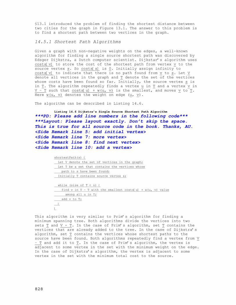
§13.1 introduced the problem of finding the shortest distance between two cities for the graph in Figure 13.1. The answer to this problem is to find a shortest path between two vertices in the graph. 14.5.1 Shortest Path Algorithms
Given a graph with non-negative weights on the edges, a well-known algorithm for finding a single source shortest path was discovered by Edsger Dijkstra, a Dutch computer scientist. Dijkstar’s algorithm uses costs[v] to store the cost of the shortest path from vertex v to the source vertex s. So costs[s] is 0. Initially assign infinity to costs[v] to indicate that there is no path found from v to s. Let V denote all vertices in the graph and T denote the set of the vertices whose costs have been found so far. Initially, the source vertex s is in T. The algorithm repeatedly finds a vertex u in T and a vertex v in V – T such that costs[u] + w(u, v) is the smallest, and moves v to T. Here w(u, v) denotes the weight on edge (u, v). The algorithm can be described in Listing 14.6.
Listing 14.6 Dijkstra’s Single Source Shortest Path Algorithm
***PD: Please add line numbers in the following code*** ***Layout: Please layout exactly. Don’t skip the space. This is true for all source code in the book. Thanks, AU. <Side Remark line 5: add initial vertex> <Side Remark line 7: more vertex> <Side Remark line 8: find next vertex> <Side Remark line 10: add a vertex>
shortestPath(s) {
Let V denote the set of vertices in the graph;
Let T be a set that contains the vertices whose
path to s have been found;
Initially T contains source vertex s;
while (size of T < n) {
find v in V – T with the smallest costs[u] + w(u, v) value
among all u in T;
add v to T;
}
} This algorithm is very similar to Prim’s algorithm for finding a minimum spanning tree. Both algorithms divide the vertices into two sets T and V - T. In the case of Prim’s algorithm, set T contains the vertices that are already added to the tree. In the case of Dijkstra’s algorithm, set T contains the vertices whose shortest paths to the source have been found. Both algorithms repeatedly find a vertex from V – T and add it to T. In the case of Prim’s algorithm, the vertex is adjacent to some vertex in the set with the minimum weight on the edge. In the case of Dijkstra’s algorithm, the vertex is adjacent to some vertex in the set with the minimum total cost to the source.

829
u
v
T
V - T
s
T contains vertices whose shortest path to s have been found
V- T contains vertices whose shortest path to s have not been found
Figure 14.8 Find a vertex u in T that connects a vertex v in V – T with the smallest costs[u] + w(u, v). The algorithm starts by adding the source vertex s into T (line 171) and set costs[s] to 0 (line 181) It then continuously adds a vertex (say v) from V – T into T. v is the vertex that is adjacent to a vertex in T with the smallest costs[u] + w(u, v). For example, there are five edges connecting vertices in T and V – T, as shown in Figure 14.8, (u, v) is the one with the smallest costs[u] + w(u, v). After v is added to T (line 214), set costs[v] to costs[u] + w(u, v) (line 215). Let us illustrate Dijkstra’s algorithm using the graph in Figure 14.9(a). Suppose the source vertex is 1. So, costs[1] is 0 and the costs for all other vertices are initially ∞, as shown in Figure 14.9(b).
5 6
10
5
8
7
7
12
7
10
8
8
1
2
3
4
5
6
0
0 1 2 3 4 5 6
costs 0
0 1 2 3 4 5 6
parent 1
(a) (b) Figure 14.9 The algorithm will find all shortest paths from source vertex 1. Initially set T contains the source vertex. Vertices 2, 0, 6, and 3 are adjacent to the vertices in T and vertex 2 is the vertex with a path of the smallest cost to source vertex 1. So add 2 to T. costs[2] now becomes 6, as shown in Figure 14.10.

830
5 6
10
5
8
7
7
12
7
10
8
8
1
2
3
4
5
6
0
0 1 2 3 4 5 6
costs 0 6
0 1 2 3 4 5 6
parent 1 1
(a) (b) Figure 14.10 Now vertices 1 and 2 are in the set T. Now T contains {1, 2}. Vertices 0, 6, and 3 are adjacent to the vertices in T and vertex 6 is the vertex with a path of the smallest cost to source vertex 1. So add 6 to T. costs[6] now becomes 7, as shown in Figure 14.11.
5 6
10
5
8
7
7
12
7
10
8
8
1
2
3
4
5
6
0
0 1 2 3 4 5 6
costs 0 6 7
0 1 2 3 4 5 6
parent -1 1 1
(a) (b) Figure 14.11 Now vertices {1, 2, 6} are in the set T. Now T contains {1, 2, 6}. Vertices 0, 5, and 3 are adjacent to the vertices in T and vertex 0 is the vertex with a path of the smallest cost to source vertex 1. So add 0 to T. costs[0] now becomes 8, as shown in Figure 14.12.
5 6
10
5
8
7
7
12
7
10
8
8
1
2
3
4
5
6
0
0 1 2 3 4 5 6
costs 8 0 6 7
0 1 2 3 4 5 6
parent 1 -1 1 1
(a) (b)

831
Figure 14.12 Now vertices {1, 2, 6, 0} are in the set T. Now T contains {1, 2, 6, 0}. Vertices 5 and 3 are adjacent to the vertices in T and vertex 3 is the vertex with a path of the smallest cost to source vertex 1. So add 3 to T. costs[3] now becomes 10, as shown in Figure 14.13.
5 6
10
5
8
7
7
12
7
10
8
8
1
2
3
4
5
6
0
0 1 2 3 4 5 6
costs 8 0 6 10 7
0 1 2 3 4 5 6
parent 1 -1 1 1 1
(a) (b) Figure 14.13 Now vertices {1, 2, 6, 0, 3} are in the set T. Now T contains {1, 2, 6, 0, 3}. Vertices 4 and 5 are adjacent to the vertices in T and vertex 5 is the vertex with a path of the smallest cost to source vertex 1. So add 5 to T. costs[5] now becomes 14, as shown in Figure 14.14.
5 6
10
5
8
7
7
12
7
10
8
8
1
2
3
4
5
6
0
0 1 2 3 4 5 6
costs 8 0 6 10 14 7
0 1 2 3 4 5 6
parent 1 -1 1 1 6 1
(a) (b) Figure 14.14 Now vertices {1, 2, 6, 0, 3, 5} are in the set T. Now T contains {1, 2, 6, 0, 3, 5}. The smallest cost for a path to connect 4 with 1 is 18, as shown in Figure 14.15.

832
5 6
10
5
8
7
7
12
7
10
8
8
1
2
3
4
5
6
0
0 1 2 3 4 5 6
costs 8 0 6 10 18 14 7
0 1 2 3 4 5 6
parent 1 -1 1 1 3 6 1
(a) (b) Figure 14.15 Now vertices {1, 2, 6, 0, 3, 5, 4} are in the set T. 14.5.2 Implementation of the Shortest Paths Algorithm
<Side Remark: shortest path tree> As you see, the algorithm essentially finds all shortest paths from a source vertex, which produces a tree rooted at the source vertex. We call this tree a single-source all shortest path tree (or simply a shortest path tree). To model this tree, define a class named ShortestPathTree that extends the Tree class, as shown in Figure 14.16. ShortestPathTree is defined as an inner class in WeightedGraph in lines 223-246 in Listing 14.2. AbstractGraph.Tree
WeightedGraph.ShortestPathTree
+costs: int[]
+ShortestPathTree(source: int, parent: int[], costs: int[])
+getCost(v: int): int +printAllPaths(): void
costs[v] stores the cost for the path from the source to v.
Constructs a shortest path tree with the specified source, parent array, and costs array.
Returns the cost for the path from the source to vertex v. Displays all paths from the soruce.
Figure 14.16 WeightedGraph.ShortestPathTree extends AbstractGraph.Tree.
The getShortestPath(int sourceVertex) method was implemented in lines 165-218 in Listing 14.2. The method first adds sourceVertex to T (line 169). T is a set that stores the vertices whose path has been found (line 167). vertices is defined as a protected data field in the AbstractGraph class, which is an array that stores all vertices in the graph. vertices.length returns the number of the vertices in the graph (line 172). Each vertex is assigned a cost. The cost of the source vertex is 0 (line 183). The cost of all other vertices is assigned infinity initially (line 181). The method needs to remove the elements from the queues in order to find the one with the smallest total cost. To keep the original queues intact, queues are cloned in line 186.

833
A vertex is added to T if it is adjacent to one of the vertices in T with the smallest cost (line 212). Such vertex is found using the following procedure:
(1) For each vertex u in T, find its incident edge e with the smallest weight to u. All the incident edges to u are stored in queues[u]. queues[u].peek() (line 194) returns the incident edge with the smallest weight. If e.v is already in T, remove e from queues[u] (line 195). After lines 193-201, queues[u].peek() returns the edge e such that e has the smallest weight to u and e.v is not in T (line 203).
(2) Compare all these edges and find the one with the smallest value on costs[u] + + e.getWeight() (line 207).
After a new vertex is added to T (line 212), the cost of this vertex is updated (line 213). Once all vertices are added to T, an instance of ShortestPathTree is created (line 217). <Side Remark: ShortestPathTree class> The ShortestPathTree class extends the Tree class (line 221). To create an instance of ShortestPathTree, pass sourceVertex, parent, and costs (lines 217). sourceVertex becomes the root in the tree. The data fields root and parent are defined in the Tree class, which is an inner class defined in AbstractGraph. <Side Remark: Dijkstra’s algorithm time complexity> Dijkstra’s algorithm is implemented essentially in the same was as Prim’s algorithm. So, the time complexity for Dijkstra’s algorithm is
|)|log|(| VEO , where |E| denotes the number of edges and |V| denotes the number of vertices. Listing 14.7 gives a test program that displays all shortest paths from Chicago to all other cities in Figure 27.1 and all shortest paths from vertex 3 to all vertices for the graph in Figure 14.1, respectively.
Listing 14.7 TestShortestPath.java
***PD: Please add line numbers in the following code*** ***Layout: Please layout exactly. Don’t skip the space. This is true for all source code in the book. Thanks, AU. <Side Remark line 3: vertices> <Side Remark line 7: edges> <Side Remark line 26: create graph1> <Side Remark line 27: shortest path> <Side Remark line 37: create edges> <Side Remark line 44: create graph2> <Side Remark line 46: print paths>
public class TestShortestPath {
public static void main(String[] args) {
String[] vertices = {"Seattle", "San Francisco", "Los Angeles",
"Denver", "Kansas City", "Chicago", "Boston", "New York",
"Atlanta", "Miami", "Dallas", "Houston"};
int[][] edges = {
{0, 1, 807}, {0, 3, 1331}, {0, 5, 2097},

834
{1, 0, 807}, {1, 2, 381}, {1, 3, 1267},
{2, 1, 381}, {2, 3, 1015}, {2, 4, 1663}, {2, 10, 1435},
{3, 0, 1331}, {3, 1, 1267}, {3, 2, 1015}, {3, 4, 599},
{3, 5, 1003},
{4, 2, 1663}, {4, 3, 599}, {4, 5, 533}, {4, 7, 1260},
{4, 8, 864}, {4, 10, 496},
{5, 0, 2097}, {5, 3, 1003}, {5, 4, 533},
{5, 6, 983}, {5, 7, 787},
{6, 5, 983}, {6, 7, 214},
{7, 4, 1260}, {7, 5, 787},
{8, 4, 864}, {8, 7, 888}, {8, 9, 661},
{8, 10, 781}, {8, 11, 810},
{9, 8, 661}, {9, 11, 1187},
{10, 2, 1435}, {10, 4, 496}, {10, 8, 781}, {10, 11, 239},
{11, 8, 810}, {11, 9, 1187}, {11, 10, 239}
};
WeightedGraph graph1 = new WeightedGraph(edges, vertices);
WeightedGraph.ShortestPathTree tree1 = graph1.getShortestPath(5);
tree1.printAllPaths();
// Display shortest paths from Chicago to Houston
System.out.print("Shortest path from Chicago to Houston: ");
java.util.Iterator iterator = tree1.pathIterator(11);
while (iterator.hasNext())
System.out.print(iterator.next() + " ");
System.out.println();
edges = new int[][]{
{0, 1, 7}, {0, 3, 9},
{1, 0, 7}, {1, 2, 9}, {1, 3, 7},
{2, 1, 9}, {2, 3, 7}, {2, 4, 7},
{3, 0, 9}, {3, 1, 7}, {3, 2, 7}, {3, 4, 9},
{4, 2, 7}, {4, 3, 9}
};
WeightedGraph graph2 = new WeightedGraph(edges, 5);
WeightedGraph.ShortestPathTree tree2 = graph2.getShortestPath(3);
tree2.printAllPaths();
}
} <Output> All shortest paths from Chicago are: A path from Chicago to Seattle: Chicago Seattle (cost: 2097) A path from Chicago to San Francisco: Chicago Denver San Francisco (cost: 2270) A path from Chicago to Los Angeles: Chicago Denver Los Angeles (cost: 2018) A path from Chicago to Denver: Chicago Denver (cost: 1003) A path from Chicago to Kansas City: Chicago Kansas City (cost: 533) A path from Chicago to Chicago: Chicago (cost: 0) A path from Chicago to Boston: Chicago Boston (cost: 983) A path from Chicago to New York: Chicago New York (cost: 787) A path from Chicago to Atlanta: Chicago Kansas City Atlanta (cost: 1397) A path from Chicago to Miami: Chicago Kansas City Atlanta Miami (cost: 2058) A path from Chicago to Dallas:

835
Chicago Kansas City Dallas (cost: 1029) A path from Chicago to Houston: Chicago Kansas City Dallas Houston (cost: 1268) Shortest path from Chicago to Houston: Chicago Kansas City Dallas Houston All shortest paths from 3 are: A path from 3 to 0:3 0 (cost: 9) A path from 3 to 1:3 1 (cost: 7) A path from 3 to 2:3 2 (cost: 7) A path from 3 to 3:3 (cost: 0) A path from 3 to 4:3 4 (cost: 9)
<End Output> The program creates a weighted graph for Figure 27.1 in line 12. It then invokes the getShortestPath(5) method to return a Path object that contains all shortest paths from vertex 5 (i.e., Chicago). Invoking printPath() on the ShortestPathTree object displays all the paths. The graphical illustration of all shortest paths from Chicago is shown in Figure 14.17. The shortest paths from Chicago to the cities are found in this order: Kansas City, New York, Boston, Denver, Dallas, Houston, Atlanta, Los Angeles, Miami, San Francisco, and Seattle.
Seattle
San Francisco
Los Angeles
Denver
Chicago
Kansas City
Houston
Boston
New York
Atlanta
Miami
661
888
1187
810Dallas
1331
2097
1003807
381
1015
1267
1663
1435
239
496
781
864
1260
983
787
214
533
5991
2
3
4
5
6
7
8
9
10
11
Figure 14.17 The shortest paths from Chicago to all other cities are highlighted. 14.6 Case Study: The Weighted Nine Tail Problem
§13.8 presented the nine tail problem and solved it using the BFS algorithm. This section presents a modification of the problem and solves it using the shortest path algorithm. The nine tail problem is to find the minimum number of the moves that lead to all coins face down. Each move flips a head coin and its neighbors. The weighted nine tail problem assigns the number of the flips as a weight on each move. For example, you can move from the

836
coins in Figure 28(a) to Figure 28(b) by flipping the three coins. So the weight for this move is 3. H T T T
H H
H H H
T H T T
T H
H H H
(a) (b) Figure 14.18 The weight for each move is the number of the flips for the move.
The weighted nine tail problem is to find the minimum number of the flips that lead to all coins face down. The problem can be reduced to finding the shortest path from a starting node to the target node in an edge-weighted graph. The graph has 512 nodes. Create an edge from node v to u if there is a move from node u to node v. Assign the number of the flips to the edge. Recall that we created two classes: NineTailApp and NineTailModel for the nine tail problem in §13.8. The NineTailApp class is responsible for user interaction and for displaying the solution and the NineTailModel class creates a graph for modeling this problem. We may reuse the same classes to solve the weighted nine tail problem. The only change is to modify the implementation of NineTailModel. For convenience, let us name the new classes WeightedNineTailApp and WeightedNineTailModel. WeightedNineTailApp is exactly the same as NineTailApp except that the word NineTailApp and NineTailModel in the code are replaced by WeightedNineTailApp and WeightedNineTailModel, respectively. The code listing is omitted. You can download WeightedNineTailApp.java from the companion Website. The public method headers in WeightedNineTailModel are the same as the ones in NineTailModel except that UnweightedGraph is replaced by WeightedGraph and Edge is replaced by WeightedEdge. Listing 14.8 gives the new implementation of the methods.
Listing 14.8 WeightedNineTailModel.java
***PD: Please add line numbers in the following code*** ***Layout: Please layout exactly. Don’t skip the space. This is true for all source code in the book. Thanks, AU. <Side Remark line 4: vertices> <Side Remark line 5: edges> <Side Remark line 7: declare a graph> <Side Remark line 8: declare a tree> <Side Remark line 12: create nodes> <Side Remark line 13: weighted edges> <Side Remark line 16: weighted graph> <Side Remark line 19: shortest path tree> <Side Remark line 23: create 512 nodes> <Side Remark line 47: Node inner class> <Side Remark line 51: construct a node> <Side Remark line 61: construct a node>

837
<Side Remark line 66: compare two nodes> <Side Remark line 80: string representation> <Side Remark line 95: create edges> <Side Remark line 105: number of flips> <Side Remark line 108: add edges> <Side Remark line 116: get adjacent node> <Side Remark line 134: flip a cell> <Side Remark line 146: shortest path> <Side Remark line 158: number of flips>
import java.util.*;
public class WeightedNineTailModel {
private List<Node> nodes = new ArrayList<Node>(); // Vertices
private List<WeightedEdge> edges =
new ArrayList<WeightedEdge>(); // Store edges
private WeightedGraph graph; // Define a graph
private WeightedGraph.Tree tree; // Define a tree
/** Construct a model */
public WeightedNineTailModel() {
createNodes(); // Create nodes
createEdges(); // Create edges
// Create a graph
graph = new WeightedGraph(edges, nodes);
// Obtain a tree rooted at the target node
tree = graph.getShortestPath(511);
}
/** Create all nodes for the graph */
private void createNodes() {
for (int k1 = 0; k1 <= 1; k1++) {
for (int k2 = 0; k2 <= 1; k2++) {
for (int k3 = 0; k3 <= 1; k3++) {
for (int k4 = 0; k4 <= 1; k4++) {
for (int k5 = 0; k5 <= 1; k5++) {
for (int k6 = 0; k6 <= 1; k6++) {
for (int k7 = 0; k7 <= 1; k7++) {
for (int k8 = 0; k8 <= 1; k8++) {
for (int k9 = 0; k9 <= 1; k9++) {
nodes.add(new Node(k1, k2, k3, k4,
k5, k6, k7, k8, k9));
}
}
}
}
}
}
}
}
}
}

838
/** Node inner class */
public static class Node {
int[][] matrix = new int[3][3];
/** Construct a Node from nine numbers */
Node(int ...numbers) { // Variable-length argument
int k = 0;
for (int i = 0; i < 3; i++) {
for (int j = 0; j < 3; j++) {
matrix[i][j] = numbers[k++];
}
}
}
/** Construct a Node from nine numbers in a 3 by 3 array */
Node(int[][] numbers) {
this.matrix = numbers;
}
/** Override the equals method to compare two nodes */
public boolean equals(Object o) {
int[][] anotherMatrix = ((Node)o).matrix;
for (int i = 0; i < 3; i++) {
for (int j = 0; j < 3; j++) {
if (matrix[i][j] != anotherMatrix[i][j]) {
return false;
}
}
}
return true; // Nodes with the same matrix values
}
/** Return a string representation for the node */
public String toString() {
StringBuilder result = new StringBuilder();
for (int i = 0; i < 3; i++) {
for (int j = 0; j < 3; j++) {
result.append(matrix[i][j] + " ");
}
result.append("\n");
}
return result.toString();
}
}
/** Create all edges for the graph */
private void createEdges() {
for (Node node : nodes) {
int u = nodes.indexOf(node); // node index
int[][] matrix = node.matrix; // matrix for the node
for (int i = 0; i < 3; i++) {

839
for (int j = 0; j < 3; j++) {
if (matrix[i][j] == 0) { // For a head cell
Node adjacentNode = getAdjacentNode(matrix, i, j);
int v = nodes.indexOf(adjacentNode);
int numberOfFlips = getNumberOfFlips(adjacentNode,
node);
// Add edge (v, u) for a legal move from node u to node v
edges.add(new WeightedEdge(v, u, numberOfFlips));
}
}
}
}
}
/** Get the adjacent node after fliping the cell at i and j */
private Node getAdjacentNode(int[][] matrix, int i, int j) {
int[][] matrixOfNextNode = new int[3][3];
for (int i1 = 0; i1 < 3; i1++) {
for (int j1 = 0; j1 < 3; j1++) {
matrixOfNextNode[i1][j1] = matrix[i1][j1];
}
}
flipACell(matrixOfNextNode, i - 1, j); // Top neighbor
flipACell(matrixOfNextNode, i + 1, j); // Bottom neighbor
flipACell(matrixOfNextNode, i, j - 1); // Left neighbor
flipACell(matrixOfNextNode, i, j + 1); // Right neighbor
flipACell(matrixOfNextNode, i, j); // Flip self
return new Node(matrixOfNextNode);
}
/** Change a valid cell from 0 to 1 and 1 to 0 */
private void flipACell(int[][] matrix, int i, int j) {
if (i >= 0 && i <= 2 && j >= 0 && j <= 2) { // Within boundary
if (matrix[i][j] == 0) {
matrix[i][j] = 1; // Flip from 0 to 1
}
else {
matrix[i][j] = 0; // Flip from 1 to 0
}
}
}
/** Return the shortest path from the specified node to the root */
public List<Node> getShortestPath(Node node) {
Iterator iterator = tree.pathIterator(nodes.indexOf(node));
LinkedList list = new LinkedList();
// Insert the vertices on the path starting from the root to list
while (iterator.hasNext())
list.addFirst(iterator.next());
return list;
}

840
/** Get the number of the flips */
private int getNumberOfFlips(Node node1, Node node2) {
int[][] matrix1 = node1.matrix;
int[][] matrix2 = node2.matrix;
int count = 0; // Count the different number of cells
for (int i = 0; i < 3; i++) {
for (int j = 0; j < 3; j++) {
if (matrix1[i][j] != matrix2[i][j]) count++;
}
}
return count;
}
} Line 19 obtains a tree that represents the shortest paths rooted at the target node 511. Line 110 adds a weighted edge to the graph. The getNumberOfFlips(node1, node2) compares node1 with node2 to return the number of different cells, which is the number of the flips for the move from node1 to node2. Key Terms
***PD: Please place terms in two columns same as in intro6e.
• Dijkstra’s algorithm • edge-weighted graph • minimum spanning tree • Prim’s algorithm • shortest path • single-source shortest path • vertex-weighted graph
Chapter Summary
• You can use adjacency matrices or priority queues to represent weighted edges.
• A spanning tree of a graph is a subgraph that is a tree and connects all vertices in the graph. You learned how to implement Prim’s algorithm for finding a minimum spanning tree.
• You learned how to implement Dijkstra’s algorithm for finding shortest paths.
Review Questions
Section 14.4 Minimum Spanning Trees 14.1 Find all minimum spanning trees for the following graph.

841
6
5 4
3
2
0
7 5
10
5
2
7
7
2
7
10
8
8
1
14.2 Is the minimum spanning tree unique if all edges have different weights? 14.3 If you use an adjacency matrix to represent weighted edges, what would be the time complexity for Prim’s algorithm? Section 14.5 The Shortest Paths 14.4 Trace Dijkstra’s algorithm for finding shortest paths from Boston to all other cities in Figure 27.1. 14.5 Is the shortest path between two vertices unique if all edges have different weights? 14.6 If you use an adjacency matrix to represent weighted edges, what would be the time complexity for Dijkstra’s algorithm? Programming Exercises Sections 14.2 14.1* (Kruskal’s algorithm) The text introduced Prim’s algorithm for finding a
minimum spanning tree. Kruskal’s algorithm is another well-known algorithm for finding a minimum spanning tree. The algorithm repeatedly finds a minimum weight edge and adds it to the tree if it does not cause a cycle. The process ends when all vertices are in the tree.
14.2* (Implementing Prim’s algorithm using adjacency matrix) The text
implements Prim’s algorithm using priority queues on adjacent edges. Implement the algorithm using adjacency matrix for weighted graphs.
14.3* (Implementing Dijkstra’s algorithm using adjacency matrix) The text
implements Dijkstra’s algorithm using priority queues on adjacent edges. Implement the algorithm using adjacency matrix for weighted graphs.
14.4*

842
(Modifying weight in the nine tail problem) In the text, we assign the number of the flips as the weight for each move. Assume that the weight is three times of the number of flips, revise the program. 14.5* (Prove or disprove) The conjecture is that both NineTailModel and
WeightedNineTailModel result in the same shortest path. Write a program to prove or disprove it.
Hint: Add a new method named depth(int v) in the AbstractGraph.Tree
class to return the depth of the v in the tree. Let tree1 and tree2 denote the trees obtained from NineTailModel and WeightedNineTailModel, respectively. If the depth of a node u in tree1 and tree2 are the same, the length of the path from u to the target is the same.
14.6** (Weighted 4×4 sixteen tail model) The weighted nine tail problem in the text uses a 3×3 matrix. Assume that you have sixteen coins placed in a 4×4 matrix. Create a new model class named WeightedTailModel16. Create an instance of the model and save the object into a file named Exercise28_6.dat. 14.7** (Weighted 4×4 sixteen tail view) Listing 27.12, NineTailApp.java, presents a view for the nine tail problem. Revise this program for the weighted 4×4 sixteen tail problem. Your program should read the model object created from the preceding exercise.