4/24/2017

1

Aggregate Supply and the Short-run

Tradeoff Between Inflation and

Unemployment

Chapter 14

8th and 9th edition

We cover…

models of aggregate supply in which output

depends positively on the price level in the short

run

the short-run tradeoff between inflation and

unemployment known as the Phillips curve

More realistic SRAS

Y

P LRAS

Y

SRAS

( )eY Y P P

eP P

In between the two extreme assumptions we considered before.

VSRAS: P = 𝐏

All wages and prices

flexible

Some wages and prices

flexible

All wages and prices

fixed

4/24/2017

2

Three models of aggregate supply -

2 models presented in the book

1. The sticky-price model

2. The imperfect-information model

3. The sticky-wage model (not in the book)

All three models imply:

( )eY Y P P

natural rate

of output

a positive

parameter

the expected

price level

the actual

price level

agg.

output

How the equation works

Y

P LRAS

Y

SRAS

( )eY Y P P

eP P

eP P

eP P

is full employment output from chapter 3 assuming

perfect competition and flexible wages and prices. Y

The sticky-wage model (not in the

book) but conveys a lesson.

Assumes that firms and workers negotiate contracts

and fix the nominal wage before they know what the

price level will turn out to be.

The nominal wage, W, they set is based on a target

real wage and the expected price level:

e

Ww

P

4/24/2017

3

The sticky-wage model

If it turns out that

eP P

eP P

eP P

then

Unemployment and output are

at their natural rates.

Actual real wage is less than the

target, firms hire more workers and

output rises above its natural rate.

Actual real wage exceeds its

target, so firms hire fewer workers

and output falls below its natural

rate.

The sticky-wage model

Implies that the real wage should be

counter-cyclical, should move in the opposite

direction as output during business cycles:

In booms, when P typically rises,

real wage should fall.

In recessions, when P typically falls,

real wage should rise.

This prediction does not come true in the real

world – which is why Mankiw dropped the theory

from the book.

The cyclical behavior of the real wage.

The real wage is pro-cyclical

Perc

en

tag

e c

han

ge

in r

eal w

ag

e

Percentage change in real GDP

-5

-4

-3

-2

-1

0

1

2

3

4

5

-3 -2 -1 0 1 2 3 4 5 6 7 8

1974 1979

1991

1972

2004

2001

1998 1965

1984

1980

1982

1990

4/24/2017

4

The imperfect-information model

Assumptions:

All wages and prices are perfectly flexible,

all markets are clear. (drops the assumption of

imperfect competition)

Each supplier produces one good and consumes

a lot of others.

Each supplier knows the nominal price of her own

good, but not all of the other goods - does not

know the overall price level.

The imperfect-information model

Supply of each good depends on its relative price:

the nominal price of the good divided by the overall

price level.

Supplier doesn’t know price level at the time she

makes her production decision, so uses the

expected price level, P e.

Suppose P rises but P e does not.

Then supplier thinks her relative price has risen, so

she produces more.

With many producers thinking this way,

Y will rise whenever P rises above P e.

The imperfect-information model, also called

the Misperceptions Theory Q: What is the best time for an individual producer to increase

production?

A: When there has been an increase in demand for her specific

product

In that case, price of the good she produces rises relative to the

goods that she consumes

Producer will want to “make hay while the sun shines” and take

advantage of relative increase in demand

Q: What will be the effect of an increase in aggregate demand (say,

from from higher M)?

A: All prices will rise

But individual producers will not be able to distinguish this increase

from a shift in specific demand

So individual producers will increase production somewhat, at least

temporarily

4/24/2017

5

The sticky-price model:

Reasons for sticky prices and wages:

Not all wages and prices are flexible

long-term contracts between firms and customers

menu costs

firms not wishing to annoy customers with frequent

price changes

Summary and implications

Y

P LRAS

Y

SRAS

( )eY Y P P

eP P

eP P

eP P

is full employment output from chapter 3 assuming

perfect competition and flexible wages and prices. Y

What shifts the curves?

Change in Pe

( )eY Y P P

( )eY Y P P

4/24/2017

6

Summary & implications

Suppose a positive AD

shock moves output

above its natural rate

(to Y2) and P rises to

P2, above the level

people had expected.

Y

P LRAS

SRAS1

SRAS equation: eY Y P P ( )

1 1

eP P

AD1

AD2 2

eP

2P

3 3

eP P

As the price level

rises, over time

P

e rises.

The SRAS shifts

up, and output

returns to its

natural rate. 1Y Y 2Y3Y

SRAS2

E

F

H

Imperfect Information - Misperceptions Theory

and the Non-neutrality of Money

Monetary policy and the misperceptions

theory

Because of misperceptions, unanticipated

monetary policy has real effects; but anticipated

monetary policy has no real effects because there

are no misperceptions

The previous slide showed the effect of an

unanticipated demand shock. For example, and

unanticipated change in the money supply.

4/24/2017

7

The Misperceptions Theory and the Nonneutrality

of Money

Anticipated changes in the money supply

If people anticipate the change in the money

supply and thus in the price level, they aren't

fooled, there are no misperception, and the

SRAS curve shifts immediately to its higher

level

So anticipated monetary is neutral in both the

short run and the long run

An anticipated increase in the money supply – go

directly from P1 to P3 - directly from point E to H.

Go directly from E to H

There is no point F

Inflation, Unemployment, and the Phillips Curve

4/24/2017

8

22

5½ % = zero inflation

23

5½ %

Unemployment and Inflation:

Is There a Trade-off?

Some economist think there is a trade-off

between inflation and unemployment

In the 1960’s such a trade-off existed. This

suggested that policymakers could choose the

combination of unemployment and inflation they

most desired

But the relationship fell apart in the following

three decades

The 1970s were a particularly bad period, with

both high inflation and high unemployment,

inconsistent with the Phillips curve

4/24/2017

9

25

1970 – 1983

What

happened?

Supply-Side Inflation

Inflation 1970 – 1983

Adverse supply shocks

Crop failures 1972-1973

Oil price increases: 1973-1974, 1979-

1980

Costs increase, prices rise, output falls,

unemployment increases

26

1961

1958

1962 1954

1959

1963 1960

1964 1967

1957 1965

1955 1956

1966

1969

1968

1978 1973

1979

1974 1980

1981 1975

1983

1982

1977

1971

1970

1972

1984

1976

12%

11

10

9

8

7

6

5

4

3

2

10 9 8 7 6 5 4 3 2 0 1

Infl

ati

on

Rate

1

Unemployment Rate in Percent

The Phillips Curve: A Historical Perspective 1960’s and 1970-80’s

4/24/2017

10

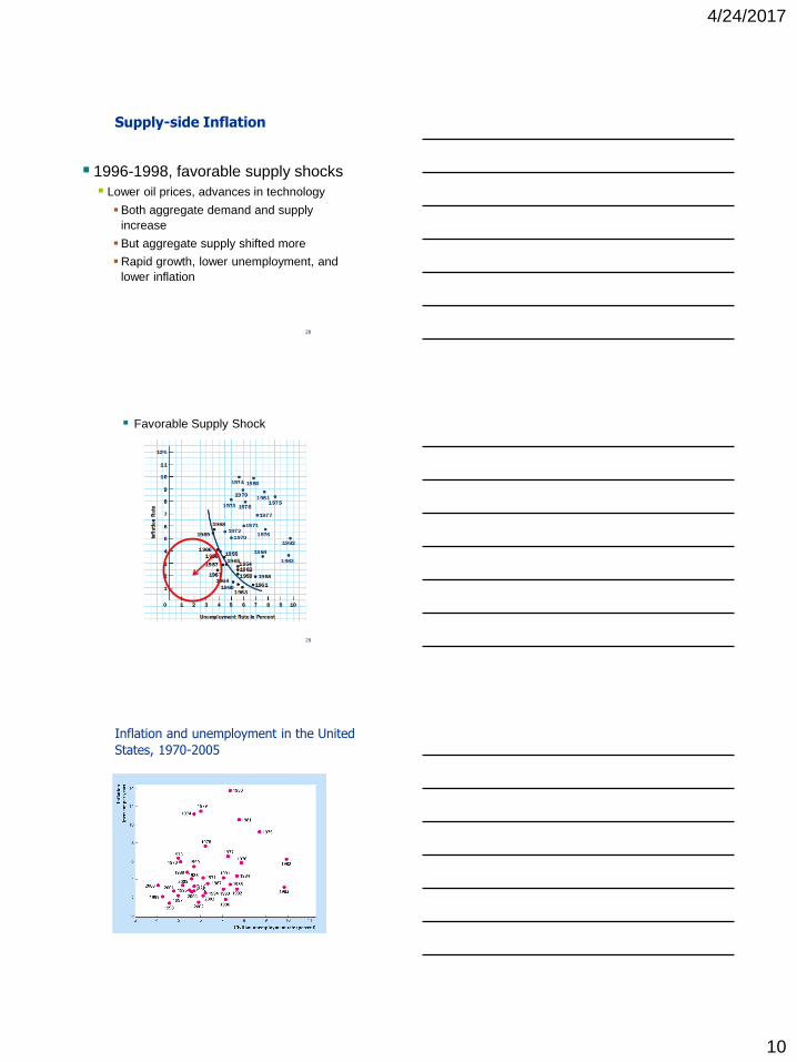
Supply-side Inflation

1996-1998, favorable supply shocks

Lower oil prices, advances in technology

Both aggregate demand and supply

increase

But aggregate supply shifted more

Rapid growth, lower unemployment, and

lower inflation

28

Favorable Supply Shock

29

Inflation and unemployment in the United

States, 1970-2005

4/24/2017

11

What the Phillips Curve Is and Is

Not

Is a statistical relationship between inflation

and unemployment

Holds if business cycle fluctuations arise

mainly from demand with AS stable

If AS shifts, the Phillips curve shifts

During 1970s, 1980s, AS was not stable.

31

The Phillips Curve is Not Stable

Self-correcting mechanism shifts the AS

curve

Refers to the way money wages respond

to recessionary or expansionary gaps

Wage changes shift the aggregate supply

curve

Effecting equilibrium real GDP and the

price level

The Phillips curve shifts

32

The Elimination of a Recessionary Gap: As the

AS curve shifts down the Phillips curve shifts

down

33

Real GDP

Pri

ce L

evel

Potential

GDP

SRAS0

SRAS0

AD

AD

SRAS1

SRAS1

SRAS2

SRAS2

A

B

C

4/24/2017

12

The Vertical Long-Run Phillips Curve

34

2 3 4 0 5 6

Unemployment Rate in Percent

7 8 9

C 1

2

3

4

5

Inflation R

ate

7

6

8%

A

PC0

PC2

The Natural Rate of Unemployment

is 5%.

PC1

B

Augmented Phillips Curve Theory

States that depends on:

expected inflation, e.

cyclical unemployment: the deviation of the actual

rate of unemployment from the natural rate

supply shocks, (Greek letter “nu”).

( ) e nu u

where > 0 is an exogenous constant.

The Phillips Curve formula is derived from

the SRAS

(1) ( )eY Y P P

(2) (1 ) ( )eP P Y Y

1 1(4) ( ) ( ) (1 )( )eP P P P Y Y

(5) (1 ) ( )e Y Y

(6) (1 ) ( ) ( )nY Y u u

(7) ( )e nu u

(3) (1 ) ( )eP P Y Y

From Okun’s Law

4/24/2017

13

The Phillips Curve and SRAS

SRAS curve: Output is related to unexpected movements in the

price level.

Phillips curve: Unemployment is related to unexpected

movements in the inflation rate.

SRAS: ( )eY Y P P

Phillips curve: e nu u ( )

How are expectations about inflation

formed? Adaptive expectations

Adaptive expectations: an approach that

assumes people form their expectations of future

inflation based on recently observed inflation.

A simple example:

Expected inflation = last year’s actual inflation

1 ( )nu u

1

e

Then, the Phillips Curve becomes

Inflation inertia

In this form, the Phillips curve implies that inflation

has inertia:

In the absence of supply shocks or cyclical

unemployment, inflation will continue indefinitely

at its current rate: π = π-1

Past inflation influences expectations of current

inflation, which in turn influences the wages &

prices that people set.

1 ( )nu u

4/24/2017

14

Two causes of rising & falling inflation

cost-push inflation:

inflation resulting from supply shocks

Adverse supply shocks typically raise production

costs and induce firms to raise prices,

“pushing” inflation up.

demand-pull inflation:

inflation resulting from demand shocks

Positive shocks to aggregate demand cause

unemployment to fall below its natural rate,

which “pulls” the inflation rate up.

1 ( )nu u

Graphing the Phillips curve

In the short

run, policymakers

face a tradeoff

between and u.

u

nu

1

The short-run

Phillips curve e

( )e nu u

Here, the “short run” is the period until people adjust their expectations of

inflation

Shifting the Phillips curve

People adjust

their

expectations

over time,

so the tradeoff

only holds in

the short run.

u

nu

1

e

( )e nu u

2

e

E.g., an increase

in e shifts the

short-run Phillips

Curve upward.

4/24/2017

15

THE COST OF REDUCING INFLATION

• To reduce inflation, policy makers can contract

aggregate demand, causing unemployment to

rise above the natural level.

• The economy must endure a period of high

unemployment and low output.

• When the Fed combats inflation, the economy

moves down the short-run Phillips curve.

• The economy experiences lower inflation but at

the cost of higher unemployment.

Example: • Consider an economy in which inflation has been steady at

13 percent per year for several years.

• Assume firms and households form their expectations on the

basis of past experience (adaptive or backward-looking

expectations) • everyone will expect inflation for the coming year to be 13

percent.

• Thus, labor negotiations will ensure a 13 percent rise in

wages. Firms expect their input costs to rise by 13 percent so

they will raise their prices by 13 percent as well.

• The Fed must be increasing the money supply 13 percent

per year as well.

Example

In this scenario, at full employment with 13% inflation.

Now, suppose the Fed wishes to break this cost-price spiral

and bring down the rate of inflation.

The only way to induce firms to raise prices by less than 13

percent is to create a situation where they are unable to sell

their output at currently planned prices.

4/24/2017

16

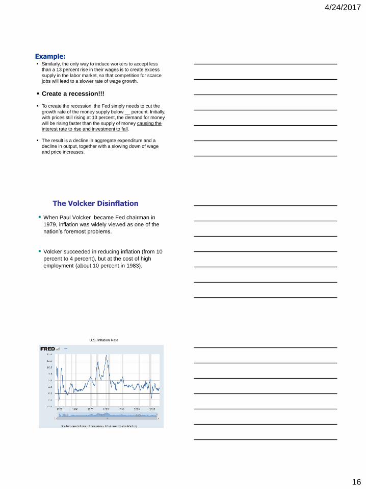
Example: Similarly, the only way to induce workers to accept less

than a 13 percent rise in their wages is to create excess

supply in the labor market, so that competition for scarce

jobs will lead to a slower rate of wage growth.

Create a recession!!!

To create the recession, the Fed simply needs to cut the

growth rate of the money supply below __ percent. Initially,

with prices still rising at 13 percent, the demand for money

will be rising faster than the supply of money causing the

interest rate to rise and investment to fall.

The result is a decline in aggregate expenditure and a

decline in output, together with a slowing down of wage

and price increases.

The Volcker Disinflation

When Paul Volcker became Fed chairman in

1979, inflation was widely viewed as one of the

nation’s foremost problems.

Volcker succeeded in reducing inflation (from 10

percent to 4 percent), but at the cost of high

employment (about 10 percent in 1983).

U.S. Inflation Rate

4/24/2017

17

The Volcker Disinflation: 1979 - 1987

1 2 3 4 5 6 7 8 9 10 0

2

4

6

8

10

Unemployment

Rate (percent)

Inflation Rate

(percent per year)

1980 1981

1982

1984

1986

1985

1979 A

1983 B

1987

C

Copyright © 2004 South-Western

The Volcker Disinflation

1 2 3 4 5 6 7 8 9 10 0

2

4

6

8

10

Unemployment

Rate (percent)

Inflation Rate

(percent per year)

1980 1981

1982

1984

1986

1985

1979 A

1983 B

1987

C

Copyright © 2004 South-Western

SRPC1

SRPC2

SRPC3

SRPC4

LRPC

The Greenspan Era

Alan Greenspan’s term as Fed chairman (1987)

began with a favorable supply shock.

In 1986, OPEC members abandoned their

agreement to restrict supply.

This led to falling inflation and falling

unemployment.

4/24/2017

18

The Greenspan Era

1 2 3 4 5 6 7 8 9 10 0

2

4

6

8

10

Unemployment

Rate (percent)

Inflation Rate

(percent per year)

1984 1991

1985

1992 1986

1993 1994

1988 1987 1995

1996 2002 1998

1999

2000 2001

1989 1990

1997

Copyright © 2004 South-Western

Rational expectations

Ways of modeling the formation of expectations:

adaptive expectations:

People base their expectations of future inflation on

recently observed inflation.

rational expectations:

People base their expectations on all available

information, including information about current and

prospective future policies. Expectations adjust

quickly.

The trade-off between inflation and unemployment

disappears quickly.

Painless disinflation?

Proponents of rational expectations believe

that the cost of reducing inflation may be very

small:

Suppose u = un and = e = 6%,

and suppose the Fed announces that it will

do whatever is necessary to reduce inflation

from 6 to 2 percent as soon as possible.

If the announcement is credible,

then e will fall, perhaps by the full 4 points.

Then, can fall without an increase in u.

4/24/2017

19

The natural rate hypothesis

The analysis of the costs of disinflation, and of

economic fluctuations in the preceding chapters,

is based on the natural rate hypothesis:

• Changes in aggregate demand affect output and

employment only in the short run.

• In the long run, the economy returns to the levels of

output, employment, and unemployment described

by the classical model (Chap. 3).

• Allows economist to study SR and LR separately.

An alternative hypothesis: Hysteresis Read the first or 5 pages of the Yellen Presentation

Hysteresis: the long-lasting influence of history

on variables such as the natural rate of

unemployment.

A recession (negative demand shock) may

increase un, so economy may not fully recover.

Hysteresis: Why negative shocks may

increase the natural rate

The skills of cyclically unemployed workers may

deteriorate while unemployed, and they may not find

a job when the recession ends.

Cyclically unemployed workers may lose their

influence on wage-setting; then, insiders (employed

workers) may bargain for higher wages for

themselves.

Result: The cyclically unemployed “outsiders”

may become structurally unemployed when the

recession ends.

4/24/2017

20

Mankiw NYT Article 11/23/13

“The most arresting piece of economic data is in the number of

weeks the average unemployed person has been looking for work

— statistics that have been compiled since 1948.

Until recently, the largest such figure was 22 weeks, in the aftermath

of the deep recession of 1981-82.

In the most recent recession, however, the average reached about

41 weeks, and it still stands at more than 36 weeks (Oct 2014 at

32.7; Oct 2015 at 28.9). In other words, after more than four years of

recovery, the economy still has an unprecedented number of long-

term unemployed.

Mankiw NYT Article 11/23/13

Some economists believe that long-term unemployment leaves

permanent scars on the economy — a theory called hysteresis.

One possible reason for hysteresis is that the long-term unemployed

lose valuable job skills and, over time, become less committed to the

labor market. In some ways, perhaps, they should be thought of as

effectively out of the labor force.

If this theory is right, the labor market today may have less slack

than the unemployment rate and the employment-to-population ratio

suggest. Policy makers at the Fed may have to accept that lower

employment is the new normal.” higher unemployment is the new

normal.

http://research.stlouisfed.org/fred2/series/LNU03008275

4/24/2017

21

Chapter Summary

1. Three models of aggregate supply in the short run:

sticky-wage model

imperfect-information model

sticky-price model

All three models imply that output rises above its

natural rate when the price level rises above the

expected price level.

Chapter Summary

2. Phillips curve

derived from the SRAS curve

states that inflation depends on

expected inflation

cyclical unemployment

supply shocks

presents policymakers with a short-run tradeoff

between inflation and unemployment

Chapter Summary

3. How people form expectations of inflation

adaptive expectations

based on recently observed inflation

implies “inertia”

rational expectations

based on all available information

implies that disinflation may be painless

4/24/2017

22

Chapter Summary

4. The natural rate hypothesis and hysteresis

the natural rate hypotheses

states that changes in aggregate demand can

only affect output and employment in the short

run

hysteresis

states that aggregate demand can have

permanent effects on output and employment