chapter 14 simplified seismic slope displacement procedures · chapter 14 simplified seismic slope...

CHAPTER 14SIMPLIFIED SEISMIC SLOPE DISPLACEMENT PROCEDURES

Jonathan D. Bray1

Dept. Civil & Environ. Engineering, Univ. of California, Berkeley, USA

Abstract. Simplified seismic slope displacement procedures are useful tools in the evaluation ofthe likely seismic performance of earth dams, natural slopes, and solid-waste landfills. Seismi-cally induced permanent displacements resulting from earthquake-induced deviatoric deformationsin earth and waste structures are typically calculated using the Newmark sliding block analogy.Some commonly used procedures are critiqued, and a recently proposed simplified procedure isrecommended for use in engineering practice. The primary source of uncertainty in assessing thelikely performance of an earth/waste structure during an earthquake is the input ground motion, sothe proposed method is based on the response of several realistic nonlinear fully coupled stick-slipsliding block models undergoing hundreds of recorded ground motions. The calculated seismic dis-placement depends primarily on the ground motion’s spectral acceleration at the degraded periodof the structure and the structure’s yield coefficient and fundamental period. Predictive equationsare provided for estimating potential seismic displacements for earth and waste structures.

1. Introduction

The failure of an earth dam, solid-waste landfill, or natural slope during an earthquakecan produce significant losses. Additionally, major damage without failure can havesevere economic consequences. Hence, the potential seismic performance of earth andwaste structures requires sound evaluation during design. Seismic evaluations of slopestability range from using relatively simple pseudostatic procedures to advanced non-linear finite element analyses. Performance is best evaluated through an assessment ofthe potential for seismically induced permanent displacements. Following largely fromthe landmark paper of Newmark (1965) sliding block analyses are utilized as part ofthe seismic evaluation of the likely performance of earth and waste structures. Simpli-fied Newmark-type procedures such as Makdisi and Seed (1978) are routinely used toprovide a rough assessment of a system’s seismic stability. Some of these proceduresare critiqued in this paper, and a recently proposed simplified method for estimatingearthquake-induced deviatoric deformations in earth and waste structures is summarizedand recommended for use in practice.

327

K.D. Pitilakis (ed.), Earthquake Geotechnical Engineering, 327–353.c© 2007 Springer.

328 Jonathan D. Bray

2. Seismic displacement analysis

2.1. CRITICAL DESIGN ISSUES

Two critical design issues must be addressed when evaluating the seismic performanceof an earth structure. First, are there materials in the structure or its foundation that willlose significant strength as a result of cyclic loading (e.g., soil liquefaction)? If so, thisshould be the primary focus of the evaluation, because large displacement flow slidescould result. The soil liquefaction evaluation procedures in Youd et al. (2001) are largelyused in practice; however, recent studies have identified deficiencies in some of theseprocedures. For example, the Chinese criteria should not be used to assess the lique-faction susceptibility of fine-grained soils. Instead, the recommendations of recent stud-ies such as Bray and Sancio (2006) based on soil plasticity (P I < 12) and sensitivity(wc/L L > 0.85) should be followed. Flow slides resulting from severe strength loss dueto liquefaction of sands and silts or post-peak strength reduction in sensitive clays are notdiscussed in this paper.

Second, if materials within or below the earth structure will not lose significant strengthas a result of cyclic loading, will the structure undergo significant deformations that mayjeopardize satisfactory performance? The estimation of seismically induced permanentdisplacements allows an engineer to address this issue. This is the design issue addressedin this paper.

2.2. DEVIATORIC-INDUCED SEISMIC DISPLACEMENTS

The Newmark sliding block model captures that part of the seismically induced per-manent displacement attributed to deviatoric shear deformation (i.e., either rigid bodyslippage along a distinct failure surface or distributed deviatoric shearing within thedeformable sliding mass). Ground movement due to volumetric compression is notexplicitly captured by Newmark-type models. The top of a slope can displace downwarddue to deviatoric deformation or volumetric compression of the slope-forming materials.However, top of slope movements resulting from distributed deviatoric straining withinthe sliding mass or stick-slip sliding along a failure surface are mechanistically differentthan top of slope movements that result from seismically induced volumetric compressionof the materials forming the slope.

Although a Newmark-type procedure may appear to capture the overall top of slope dis-placement for cases where seismic compression due to volumetric contraction of soil orwaste is the dominant mechanism, this is merely because the seismic forces that producelarge volumetric compression strains also often produce large calculated displacements ina Newmark method. This apparent correspondence should not imply that a sliding blockmodel should be used to estimate seismic compression displacements due to volumetricstraining. There are cases where the Newmark method does not capture the overall topof slope displacement, such as the seismic compression of large compacted earth fills(e.g., Stewart et al., 2001). Deviatoric-induced deformation and volumetric-induced

Simplified seismic slope displacement procedures 329

deformation should be analyzed separately by using procedures based on the slidingblock model to estimate deviatoric-induced displacements and using other procedures(e.g., Tokimatsu and Seed, 1987) to estimate volumetric-induced seismic displacements.

The calculated seismic displacement from Newmark-type procedures, whether the pro-cedure is simplified or advanced, is viewed appropriately as an index of seismic perfor-mance. Seismic displacement estimates will always be approximate in nature due to thecomplexities of the dynamic response of the earth/waste materials involved and the vari-ability of the earthquake ground motion. However, when viewed as an index of potentialseismic performance, the calculated seismic displacement can and has been used effec-tively in practice to evaluate earth/waste structure designs.

3. Components of a seismic displacement analysis

3.1. GENERAL

The critical components of a seismic displacement analysis are: (1) earthquake groundmotion, (2) dynamic resistance of the structure, and (3) dynamic response of the potentialsliding mass. The earthquake ground motion is the most important of these componentsin terms of its contribution to the calculation of the amount of seismic displacement. Thevariability in calculated seismic displacement is primarily controlled by the significantvariability in the earthquake ground motion, and it is relatively less affected by the vari-ability in the earth slope properties (e.g., Yegian et al., 1991b; Kim and Sitar, 2003).The dynamic resistance of the earth/waste structure is the next key component, and thedynamic response of the potential sliding mass is generally third in importance. Otherfactors, such as the method of analysis, topographic effects, etc., can be important forsome cases. However, these three components are most important for a majority of cases.In critiquing various simplified seismic displacement procedures it is useful to comparehow each method characterizes the earthquake ground motion and the earth/waste struc-ture’s dynamic resistance and dynamic response.

3.2. EARTHQUAKE GROUND MOTION

An acceleration-time history provides a complete definition of one of the many possi-ble earthquake ground motions at a site. Simplified parameters such as the peak groundacceleration (PGA), mean period (Tm), and significant duration (D5–95) may be usedin simplified procedures to characterize the intensity, frequency content, and duration,respectively, of an acceleration-time history. Preferably, all three, and at least two, ofthese simplified ground motion parameters should be used. It is overly simplistic to char-acterize an earthquake ground motion by just its PGA, because ground motions withidentical PGA values can vary significantly in terms of frequency content and duration,and most importantly in terms of its effects on slope instability. Hence, PGA is typi-cally supplemented by additional parameters characterizing the frequency content andduration of the ground motion. For example, Makdisi and Seed (1978) use earthquake


magnitude as a proxy for duration in combination with the estimated PGA at the crest ofthe embankment; Yegian et al. (1991b) use predominant period and equivalent number ofcycles of loading in combination with PGA; and Bray et al. (1998) use the mean periodand significant duration of the design rock motion in combination with its PGA.

Spectral acceleration has been commonly employed in earthquake engineering to char-acterize an equivalent seismic loading on a structure from the earthquake ground motion.Similarly, Travasarou and Bray (2003a) found that the 5% damped elastic spectral accel-eration at the degraded fundamental period of the potential sliding mass was the optimalground motion intensity measure in terms of efficiency and sufficiency (i.e., it minimizesthe variability in its correlation with seismic displacement, and it renders the relationshipindependent of other variables, respectively, Cornell and Luco, 2001). The efficiencyand sufficiency of estimating seismic displacement given a ground motion intensitymeasure were investigated for dozens of intensity measures. Other promising groundmotion parameters included PGA, spectral acceleration (Sa), root mean square acceler-ation (arms), peak ground velocity (PGV), Arias intensity (Ia), effective peak velocity(EPV), Housner’s response spectrum intensity (SI), and Ang’s characteristic intensity(Ic). For period-independent parameters (i.e., no knowledge of the fundamental periodof the potential sliding mass is required), Arias intensity was found to be the most effi-cient intensity measure for a stiff, weak slope, and response spectrum intensity was foundto be the most efficient for a flexible slope.

No one period-independent ground motion parameter, however, was found to be ade-quately efficient for slopes of all dynamic stiffnesses and strengths. Spectral accelera-tion at a degraded period equal to 1.5 times the initial fundamental period of the slope(i.e., Sa(1.5Ts)) was found to be the most efficient ground motion parameter for all slopes(Travasarou and Bray, 2003a). An estimate of the initial fundamental period of the poten-tial sliding mass (Ts) is required when using spectral acceleration, but an estimate of Ts isuseful in characterizing the dynamic response aspects of the sliding mass (e.g., Bray andRathje, 1998). Spectral acceleration does directly capture the important ground motioncharacteristics of intensity and frequency content in relation to the degraded naturalperiod of the potential sliding mass, and it indirectly partially captures the influence ofduration in that it tends to increase as earthquake magnitude (i.e., duration) increases. Anadditional benefit of selecting spectral acceleration to represent the ground motion is thatspectral acceleration can be computed relatively easily due to the existence of severalattenuation relationships and it is available at various return periods in ground motionhazard maps (e.g., http://earthquake.usgs.gov/research/hazmaps/).

3.3. DYNAMIC RESISTANCE

The earth/waste structure’s yield coefficient (ky) represents its overall dynamic resis-tance, which depends primarily on the dynamic strength of the material along the criticalsliding surface and the structure’s geometry and weight. The yield coefficient parameterhas always been used in simplified sliding block procedures due to its important effect onseismic displacement.


The primary issue in calculating ky is estimating the dynamic strength of the criticalstrata within the slope. Several publications include extensive discussions of the dynamicstrength of soil (e.g., Blake et al., 2002; Duncan and Wright, 2005; Chen et al., 2006), anda satisfactory discussion of this important topic is beyond the scope of this paper. Need-less to say, the engineer should devote considerable resources and attention to developingrealistic estimates of the dynamic strengths of key slope materials. In this paper, it isassumed that ky is constant, so consequently, the earth materials do not undergo severestrength loss as a result of earthquake shaking (e.g., no liquefaction).

Duncan (1996) found that consistent (and assumed to be reasonable) estimates of aslope’s static factor of safety (FS) are calculated if a slope stability procedure that sat-isfies all three conditions of equilibrium is employed. Computer programs that utilizesuch methods as Spencer, Generalized Janbu, and Morgenstern and Price may be usedto develop sound estimates of the static FS. Most programs also allow the horizontalseismic coefficient that results in a F S = 1.0 in a pseudostatic slope stability analysisto be calculated, and if a method that satisfied full equilibrium is used, the estimates ofky are fairly consistent. With the wide availability of these computer programs and theirease of use, there is no reason to use a computer program that incorporates a method thatdoes not satisfy full equilibrium. Simplified equations for calculating ky as a functionof slope geometry, weight, and strength are found in Bray et al. (1998) among severalother works. The equations provided in Figure 14.1 may be used to estimate ky for thesimplified procedures presented in this paper.

The potential sliding mass that has the lowest static FS may not be the most critical fordynamic analysis. A search should be made to find sliding surfaces that produce low ky

values as well. The most important parameter for identifying critical potential slidingmasses for dynamic problems is ky/kmax , where kmax is the maximum seismic coeffi-cient, which represents the maximum seismic loading considering the dynamic responseof the potential sliding mass as described next.

H

c = cohesionφ = friction angle

1S2

1 HS1

Lq1 = tan

−1(1/S1)

γ . H . cos2 b . (1+tanf .tanb )

cky = tan (f − b ) + cosq1

. sinq1. S1

.H/2tan f . (S1 .H/2 . cos2q1+L+S2 . H/2)

FSstatic =

(FSstatic−1) . cosq1. sinq1

. S1. H/2

H . (S1+S2)/2+Lky =

(a) (b)

β

Fig. 14.1. Simplified estimates of the yield coefficient: (a) shallow slidingand (b) deep sliding


3.4. DYNAMIC RESPONSE

Research by investigators (e.g., Bray and Rathje, 1998) has found that seismic displace-ment also depends on the dynamic response characteristics of the potential sliding mass.With all other factors held constant, seismic displacements increase when the sliding massis near resonance compared to that calculated for very stiff or very flexible slopes (e.g.,Kramer and Smith, 1997; Rathje and Bray, 2000; Wartman et al., 2003). Many of theavailable simplified slope displacement procedures employ the original Newmark rigidsliding block assumption (e.g., Lin and Whitman, 1986; Ambraseys and Menu, 1988;Yegian et al., 1991b), which does not capture the dynamic response of the deformableearth/waste potential sliding mass during earthquake shaking.

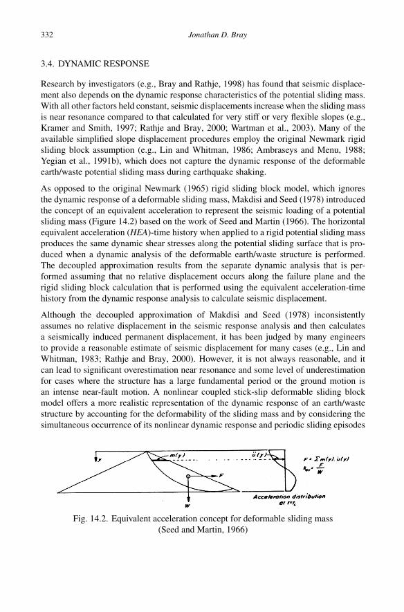
As opposed to the original Newmark (1965) rigid sliding block model, which ignoresthe dynamic response of a deformable sliding mass, Makdisi and Seed (1978) introducedthe concept of an equivalent acceleration to represent the seismic loading of a potentialsliding mass (Figure 14.2) based on the work of Seed and Martin (1966). The horizontalequivalent acceleration (HEA)-time history when applied to a rigid potential sliding massproduces the same dynamic shear stresses along the potential sliding surface that is pro-duced when a dynamic analysis of the deformable earth/waste structure is performed.The decoupled approximation results from the separate dynamic analysis that is per-formed assuming that no relative displacement occurs along the failure plane and therigid sliding block calculation that is performed using the equivalent acceleration-timehistory from the dynamic response analysis to calculate seismic displacement.

Although the decoupled approximation of Makdisi and Seed (1978) inconsistentlyassumes no relative displacement in the seismic response analysis and then calculatesa seismically induced permanent displacement, it has been judged by many engineersto provide a reasonable estimate of seismic displacement for many cases (e.g., Lin andWhitman, 1983; Rathje and Bray, 2000). However, it is not always reasonable, and itcan lead to significant overestimation near resonance and some level of underestimationfor cases where the structure has a large fundamental period or the ground motion isan intense near-fault motion. A nonlinear coupled stick-slip deformable sliding blockmodel offers a more realistic representation of the dynamic response of an earth/wastestructure by accounting for the deformability of the sliding mass and by considering thesimultaneous occurrence of its nonlinear dynamic response and periodic sliding episodes

Fig. 14.2. Equivalent acceleration concept for deformable sliding mass(Seed and Martin, 1966)


Earth Fill

Potential Slide Plane

Decoupled Analysis

Coupled Analysis

Flexible System

Dynamic Response

Rigid Block

Sliding Response

Dynamic Response and Sliding Response

Max Force atBase = ky·W

Calculate HEA-time history

assuming no sliding along base

Doubleintegrate HEA-

time historygiven ky to calculate U

Flexible System

Fig. 14.3. Decoupled dynamic response/rigid sliding block analysisand fully coupled analysis

(a) Ts = 4 H / Vs

Ts = 4 H / Vs

(b)

EARTH FILL H

Potential Slide Plane

H

(c)

H

Ts = 2.6 H / Vs

Fig. 14.4. Estimating the initial fundamental period of potential sliding blocks

(Figure 14.3). In addition, its validation against shaking table experiments providesconfidence in its use (Wartman et al., 2003).

For seismic displacement methods that incorporate the seismic response of a deformablesliding block, the initial fundamental period of the sliding mass (Ts) can normally beestimated using the expression: Ts = 4H/Vs for the case of a relatively wide potentialsliding mass that is either shaped like a trapezoid or segment of a circle where its responseis largely 1D (e.g., Rathje and Bray, 2001), where H = the average height of the potentialsliding mass, and Vs is the average shear wave velocity of the sliding mass. For the specialcase of a triangular-shaped sliding mass that largely has a 2D response, the expression:Ts = 2.6H/Vs should be used. Examples of the manner in which Ts should be estimatedare shown in Figure 14.4.


4. Critique of some simplified seismic displacement methods

4.1. GENERAL

Comprehensive discussions of seismic displacement procedures for evaluating the seis-mic performance of earth/waste structures have been presented previously by severalinvestigators (e.g., Makdisi and Seed, 1978; Seed, 1979; Lin and Whitman, 1983;Ambraseys and Menu, 1988; Yegian et al., 1991a, b; Marcuson et al., 1992; Jibson, 1993;Ambraseys and Srbulov, 1994; Bray et al., 1995; Ghahraman and Yegian, 1996; Kramerand Smith, 1997; Bray and Rathje, 1998; Finn, 1998; Jibson et al., 1998; Rathje and Bray,2000; Stewart et al., 2003; Rathje and Saygili, 2006). There is not sufficient space in thispaper to summarize and critique all pertinent studies. In this paper, some of the mostcommonly used simplified procedures for evaluating seismic displacement of earth andwaste fills will be discussed with a focus on methods that do not assume that potentialsliding mass is rigid.

4.2. SEED (1979) PSEUDOSTATIC SLOPE STABILITY PROCEDURE

First, several simplified pseudostatic slope stability procedures are commonly used inpractice. They include Seed (1979) and the Hynes-Griffin and Franklin (1984). Bothmethods involve a number of simplifying assumptions and are both calibrated for eval-uating earth dams wherein they assumed that <1 m of seismic displacement constitutedacceptable performance. They should not be applied to cases where seismically inducedpermanent displacements of up to 1 m are not acceptable, which is most cases for eval-uating base sliding of lined solid-waste landfills or houses built atop compacted earthfill slopes. Additionally, they provide a limited capability to assess seismic performance,because they do not directly address the key performance index of calculated seismicdisplacement.

The Seed (1979) pseudostatic slope stability method was developed for earth dams withmaterials that do not undergo severe strength loss that have crest accelerations lessthan 0.75 g. Using a seismic coefficient of 0.15 with appropriate dynamic strengths forthe critical earth materials, performance is judged to be acceptable if F S> 1.15. Thecharacteristics of the earthquake ground motion and the dynamic response of the poten-tial slide mass to the earthquake shaking are represented by the seismic coefficient of 0.15for all cases. Use of F S>1.15 ensures that the yield coefficient (i.e., dynamic resistanceof the earth dam) will be greater than 0.15 by an unknown amount. Thus, the earthquakeground motion and dynamic resistance and dynamic response of the earth dam are verysimply captured in this approach, and the amount of conservatism involved in the estimateand the expected seismic performance is uncertain. An earth structure that satisfies theSeed (1979) recommended combination of seismic coefficient, FS, and dynamic strengthsmay displace up to 1 m, so satisfaction of this criteria does not mean the system is “safe”for all levels of performance.


4.3. MAKDISI AND SEED (1978) SIMPLIFIED SEISMICDISPLACEMENT METHOD

The first step in the widely used Makdisi and Seed (1978) approach is the evaluationof the material’s strength loss potential. They recommend not using their procedure ifthe loss of material strength could be significant. If only a minor amount of strengthloss is likely, a slightly reduced shear strength, which often incorporates a 10% to 20%strength reduction from peak undrained shear strength, is recommended. The strengthreduction is applied because of the use of a rigid, perfectly plastic sliding block model,wherein if peak strength was used the accumulation of nonlinear elasto-plastic strainsfor cyclic loads below peak would be significantly underestimated (i.e., zero vs. somenominal amount). Based on these slightly reduced best estimates of calibrated dynamicstrengths and slope geometry and weight, ky is then calculated in the second step.

In step three, the PGA that occurs at the crest of the earth structure is estimated. This isone of the greatest limitations of this method. As shown in Figure 14.5, which presentsresults of 1D SHAKE analyses of columns of waste placed atop a firm foundation for anumber of ground motions, the PGA (or maximum horizontal acceleration, MHA) at thetop of the landfill varies significantly. There is great uncertainty regarding what value ofPGA to use. This is critical, because in the next step, the maximum seismic coefficient(kmax ) is estimated as a function of the PGA at the crest and the depth of sliding belowthe crest. Thus, the uncertainty in the estimate of kmax is high, because the uncertainty

Fig. 14.5. Maximum horizontal acceleration at top of waste fill vs. MHA of rock base(Bray and Rathje, 1998)


0

0.2

Average ofall data

O F.E. Method

“Shear Slice”(range for all data)

0.4

y/h

0.6

0.8

1.00 0.2 0.4 0.6 0.8 1.0

kmax / PGA/g

Fig. 14.6. Estimating seismic coefficient as a function of the peak acceleration at thecrest and the depth of sliding (Makdisi and Seed, 1978)

in estimating the crest PGA is high. Even with advanced analyses, estimating the crestPGA is difficult, and the need to perform any level of dynamic analysis to estimate thecrest PGA conflicts with the intent of a simplified method that should not require moreadvanced analysis.

Moreover, the bounds shown on the Makdisi and Seed (1978) plot of kmax/PG A vs. y/h(Figure 14.6) are not true upper or lower bounds. Stiff earth structures undergoing groundmotions with mean periods near the degraded period of the earth structure can have kmax

values exceeding 50% of the crest PGA for the base sliding case (i.e., y/h = 1.0), andflexible earth structures undergoing ground motions with low mean periods can have kmax

values less than 20% of the crest PGA for base sliding.

When typically used in practice, the final step is to estimate seismic displacement as afunction of the ratio of ky/kmax and earthquake magnitude. Again the range shown inFigure 14.7 does not constitute the true upper and lower bounds of the possible seismicdisplacement, as only a limited number of earth structures were analyzed with a verylimited number of input ground motions. As recommended by Makdisi and Seed (1978):“It must be noted that the design curves presented are based on averages of a range ofresults that exhibit some degree of scatter and are derived from a limited number of cases.These curves should be updated and refined as analytical results for more embankmentsare obtained.” Similar to how the Seed and Idriss (1971) simplified liquefaction trigger-ing procedure was updated through Seed et al. (1985) and then Youd et al. (2001), it istime to update and move beyond the Makdisi and Seed (1978) design curves.


1000

100

10

1

0.1

0.010 0.2 0.4 0.6 0.8 1.0

M = 8 1/4

M = 6 1/2

M = 7 1/2

DIS

PL

AC

EM

EN

T, U

(CM

)

ky/kmax

Fig. 14.7. Seismic displacement vs. ky/kmax and magnitude (Makdisi and Seed, 1978)

The Makdisi and Seed (1978) simplified seismic displacement method is one of themost significant contributions to geotechnical earthquake engineering over the past fewdecades. But as they recommended, their design curves should be updated as the profes-sion advances. Since 1989, the number of recorded ground motions has increased dra-matically. Thousands of well recorded ground motions are now available. The Makdisiand Seed (1978) work is based on a limited number of recorded and modified groundmotions. Moreover, the important earthquake ground motion at a site is characterized bythe PGA at the crest of the slope and earthquake magnitude. The PGA at the crest of theslope is highly variable and important frequency content aspects of the ground motion arenot captured. The analytical method employed was relatively simple (e.g., primarily theshear slice method and a few equivalent-linear 2D finite element analyses). The decou-pled approximation was employed, there is no estimate of uncertainty, and the boundsshown in the design curves are not true upper and lower bounds.

4.4. BRAY ET AL. (1998) SIMPLIFIED SEISMIC DISPLACEMENT APPROACH

The Bray et al. (1998) method is largely based on the work of Bray and Rathje (1998)which in turn follows on the works of Seed and Martin (1966), Makdisi and Seed (1978),and Bray et al. (1995). The methodology is based on the results of fully nonlineardecoupled one-dimensional D-MOD (Matasovic and Vucetic, 1995) dynamic analysescombined with the Newmark rigid sliding block procedure. To address the importanceof the dynamic response characteristics of the sliding mass, six fill heights with threeshear wave velocity profiles each with multiple unit weight profiles and two sets ofstrain-dependent shear modulus reduction and material damping relationships were used.


More importantly, taking advantage of the greater number of recorded earthquake groundmotions available at the time, dozens of dissimilar scaled and unmodified recorded earth-quake rock input motions were used with PGAs ranging from 0.2 g to 0.8 g. Their methodwas calibrated against several case histories of waste fill performance during the 1989Loma Prieta and 1994 Northridge earthquakes, and later validated against observed earthfill performance.

The Bray et al. (1998) procedure provides a more comprehensive assessment of the earth-quake ground motions, seismic loading, and seismic displacement calculations, but itrequires more effort than the Makdisi and Seed (1978) procedure. In the first step, theground motion is characterized by estimating the MHA, Tm , and D5–95 for outcroppingrock at the site given the assigned design moment magnitude and distances for the identi-fied key potential seismic sources. The intensity, frequency content, and duration for themedian earthquake ground motion level for deterministic events are estimated using sev-eral available ground motion parameter empirical relationships (e.g., Figure 14.8). Therock site condition is used, which is also consistent with the site condition used in thedevelopment of probabilistic ground motion hazard maps. Additionally, a seismic siteresponse analysis is not required to estimate the PGA at the top of slope.

For the deep sliding case, the initial fundamental period of the potential sliding mass (Ts)is estimated as discussed previously (i.e., Ts ≈ 4H/Vs). With the ratio of Ts/Tm , the nor-malized maximum seismic loading (i.e., (M H E A)/((M H Arock)(N RF)), where MHEAis the maximum horizontal equivalent acceleration and NRF is the nonlinear responsefactor) can be estimated with the graph shown in Figure 14.9, or the equation providedbelow, when Ts/Tm > 0.5

ln(M H E A/(M H Arock N RF)) = −0.624 − 0.7831 ln(Ts/Tm)± ε (14.1)

1 10 100Distance (km)

0.01

0.1

1

MH

A (

g)

Mw 6.0

Mw 7.0

Mw 8.0

0 20 40 60 80 100Distance (km)

0.0

0.2

0.4

0.6

0.8

1.0

Tm

(s)

0 20 6040 80 100Distance (km)

0

10

20

30

40

50

60

Sig

nific

ant d

urat

ion,

D5−95

(s)

(b) (c)(a)

Strike slipevent

Fig. 14.8. Simplified characterization of earthquake rock motions: (a) intensity—MHAfor strike-slip faults (for reverse faults, use 1.3∗M H A for Mw ≥ 6.4 and 1.64∗M H Afor Mw = 6.0, with linear interpolation for 6.0 < Mw < 6.4) (Abrahamson and Silva,

1997), (b) frequency content—Tm (Rathje et al., 2004), and (c) duration—D5–95(Abrahamson and Silva, 1996)


0.0 1.0 2.0 3.0 4.0 5.0 6.0 7.0 8.0Ts-waste/Tm-eq

0.00.20.40.60.81.01.21.41.61.82.0

MH

EA

/(M

HA

, roc

k*N

RF

) Rock site median, and 16th and 84thprobability of exceedance lines

0.1 1.350.2 1.200.3 1.090.4 1.000.5 0.920.6 0.870.7 0.820.8 0.78

MHA, rock (g) NRF

Fig. 14.9. Normalized maximum horizontal equivalent acceleration vs. normalizedfundamental Period of sliding mass (Bray and Rathje, 1998)

0.0 0.2 0.4 0.6 0.8 1.0ky/kmax

0.001

0.01

0.1

1

10

100

1000

Nor

mal

ized

Bas

e L

iner

Slid

ing

Displ

acem

ent

(U/k

max

*D5-

95, cm

/sec

)

Mw 6.25 - Std. Error 0.35



log(U/kmax*D5-95) = 1.87-3.477*ky/kmax, Std. Error 0.35

Full Data Set Regression

16% and 84% prob. of exceedance

5% and 95% prob. of exceedance

Fig. 14.10. Normalized base liner sliding displacements (from Bray and Rathje, 1998)

where σ = 0.298. The seismic coefficient kmax = M H E A/g. With an estimate of ky ,the normalized seismic displacement can be estimated as a function of ky/kmax usingFigure 14.10, or this equation

log10(U/(kmax D5–95)) = 1.87 − 3.477(ky/kmax )± ε (14.2)


where σ = 0.35. The seismic displacement (U in cm) can then be estimated by multi-plying the normalized seismic displacement value by the median estimates of kmax andD5–95. The normalized seismic loading and displacement values are estimated at themedian and 16% exceedance levels to develop a range of estimated seismic displace-ments.

The Bray et al. (1998) seismic slope displacement procedure provides median and stan-dard deviation estimates of the seismic demand and normalized seismic displacement,but does so only in an approximate manner to develop a sense of the variability of theestimated displacement. It is limited in that it was not developed in a rigorous probabilis-tic manner. However, Stewart et al. (2003) were able to use this procedure to developa probabilistic screening analysis for deciding if detailed project-specific seismic slopestability investigations are required by the 1990 California Seismic Hazards MappingAct. Additionally, the Bray and Rathje (1998) simplified seismic displacement proce-dure was adopted in the guidance document by Blake et al. (2002) for evaluating seismicslope stability in conformance with the “Guidelines for Evaluating and Mitigating Seis-mic Hazards in California” (CDMG, 1997).

As noted previously, the Bray et al. (1998) method is also limited by the decoupledapproximation employed in the seismic response and Newark sliding block calculations.Although many more ground motions were used than were used by Makdisi and Seed(1978), with the large number of well-recorded events since 1998, significantly moreground motions are now available. These shortcomings motivated a more recent study,which is summarized in the next section of this paper.

5. Bray and Travasarou (2007) simplified seismic displacement procedure

5.1. EARTHQUAKE GROUND MOTIONS

Currently available simplified slope displacement estimation procedures were largelydeveloped based on a relatively modest number of earthquake recordings or simulations.This study took advantage of the recently augmented database of earthquake recordings,which provides the opportunity to characterize better the important influence of groundmotions on the seismic performance of an earth/waste slope. As discussed previously, theuncertainty in the ground motion characterization is the greatest source of uncertainty incalculating seismic displacements.

The ground motion database used by Bray and Travasarou (2007) to generatethe seismic displacement data comprises available records from shallow crustalearthquakes that occurred in active plate margins (PEER strong motion database〈http://peer.berkeley.edu/smcat/index.html〉). These records conform to the followingcriteria: (1) 5.5 ≤ Mw ≤ 7.6, (2) R ≤ 100 km, (3) Simplified Geotechnical Sites B, C, orD (i.e., rock, soft rock/shallow stiff soil, or deep stiff soil, respectively, Rodriguez-Mareket al., 2001), and (4) frequencies in the range of 0.25 to 10 Hz have not been filteredout. Earthquake records totaling 688 from 41 earthquakes comprise the ground motion


database for this study (see Travasarou, 2003 for a list of records used). The two horizon-tal components of each record were used to calculate an average seismic displacement foreach side of the records, and the maximum of these values was assigned to that record.

5.2. DYNAMIC RESISTANCE OF THE EARTH/WASTE STRUCTURE

The seismic coefficient is calculated as described before using a computer program thathas a slope stability method that satisfies all three conditions of equilibrium, or for prelim-inary analyses, a simplified estimate of ky can be calculated using the equations providedpreviously in Figure 14.1.

5.3. DYNAMIC RESPONSE OF THE POTENTIAL SLIDING MASS

The nonlinear coupled stick-slip deformable sliding model proposed by Rathje and Bray(2000) for one-directional sliding was used by Bray and Travasarou (2007). The seis-mic response of the sliding mass is captured by an equivalent-linear viscoelastic modalanalysis that uses strain-dependent material properties to capture the nonlinear responseof earth and waste materials. It considers a single mode shape, but the effects of includ-ing three modes were shown to be small. The results from this model have been shownto compare favorably with those from a fully nonlinear D-MOD-type stick-slip analysis(Rathje and Bray, 2000), but this model can be utilized in a more straightforward andtransparent manner. The model used is one-dimensional (i.e., a relatively wide verticalcolumn of deformable soil) to allow for the use of a large number of ground motions withwide range of properties of the potential sliding mass in this study. One-dimensional(1D) analysis has been found to provide a reasonably conservative estimate of thedynamic stresses at the base of two-dimensional (2D) sliding systems (e.g., Vrymoedand Calzascia, 1978; Elton et al., 1991) and the calculated seismic displacements (Rathjeand Bray, 2001). However, 1D analysis can underestimate the seismic demand for shal-low sliding at the top of 2D systems where topographic amplification is significant. Forthis case, the seismic loading (which can be approximated by PGA for the shallow slid-ing case) can be amplified as recommended by Rathje and Bray (2001) for moderatelysteep slopes (i.e., ∼1.25 PGA) and as recommended by Ashford and Sitar (2002) forsteep (>60◦) slopes (i.e., ∼1.5 PGA).

The nonlinear coupled stick-slip deformable sliding model of Rathje and Bray (2000)can be characterized by: (1) its strength as represented by its yield coefficient, ky , (2) itsdynamic stiffness as represented by its initial fundamental period, Ts , (3) its unit weight,and (4) its strain-dependent shear modulus and damping curves. Seismic displacementvalues were generated by computing the response of the idealized sliding mass modelwith 10 values of its yield coefficient from 0.02 to 0.4 and with 8 values of its initial fun-damental period from 0 to 2 s to the entire set of recorded earthquake motions describedpreviously. Unit weight was set to 18 kN/m3, and the Vucetic and Dobry (1991) shearmodulus reduction and damping curves for a PI = 30 material were used. For the base-line case, the overburden-stress corrected shear wave velocity (Vs1) was set to 250 m/s,


and the shear wave velocity profile of the sliding block was developed using the rela-tionship that shear wave velocity (Vs) is proportional to the fourth-root of the verticaleffective stress. The sliding block height (H) was increased until the specified value ofTs was obtained. For common Ts values from 0.2 to 0.7 s, another reasonable combinationof H and average Vs were used to confirm that the results were not significantly sensitiveto these parameters individually. For nonzero Ts values, H varied between 12 and 100 m,and the average Vs was between 200 and 425 m/s. Hence, realistic values of the initialfundamental period and yield coefficient for a wide range of earth/waste fills were used.

5.4. FUNCTIONAL FORMS OF MODEL EQUATIONS

Situations commonly arise where a combination of earthquake loading and slope prop-erties will result in no significant deformation of an earth/waste system. Consequently,the finite probability of obtaining negligible (“zero”) displacement should be modeledas a function of the independent random variables. Thus, during an earthquake, an earthslope may experience “zero” or finite permanent displacements depending on the char-acteristics of the strong ground motion and the slope’s dynamic properties and geometry.As discussed in Travasarou and Bray (2003b), seismically induced permanent displace-ments can be modeled as a mixed random variable, which has a certain probability massat zero displacement and a probability density for finite displacement values. Displace-ments smaller than 1 cm are not of engineering significance and can for practical purposesbe considered as negligible or “zero.” Additionally, the regression of displacement as afunction of a ground motion intensity measure should not be dictated by data at negligiblelevels of seismic displacement.

Contrary to a continuous random variable, the mixed random variable can take on dis-crete outcomes with finite probabilities at certain points on the line as well as outcomesover one or more continuous intervals with specified probability densities. The values ofseismic displacement that are smaller than 1 cm are lumped to d0 = 1 cm. The probabilitydensity function of seismic displacement is then

fD(d) = p̃δ(d − d0)+ (1 − p̃) f̃D(d) (14.3)

where fD(d) is the displacement probability density function; p̃ is the probability mass atD = d0; δ(d − d0) is the Dirac delta function; and f̃D(d) is the displacement probabilitydensity function for D > d0.

The predictive model for seismic displacement consists of two discrete steps. First, theprobability of occurrence of “zero” displacement (i.e., D ≤ 1 cm) is computed as a func-tion of the primary independent variables ky , Ts , and Sa(1.5Ts). The dependence of theprobability of “zero” displacement on the three independent variables is illustrated inFigure 14.11. The probability of “zero” displacement increases significantly as the yieldcoefficient increases, and decreases significantly as the ground motion’s spectral accelera-tion at the degraded period of the slope increases. The probability of “zero” displacementdecreases initially as the fundamental period increases from zero, because the slope is


1

0.8

0.6

0.4

0.2

0

1

0.8

0.6

0.4

0.2

0

0.01 0.1 0.5 0.01 0.1 1 101.5 20

Yield Coefficent Fundamental Period (s) Sa(1.5Ts) (g)

P(D

="0

")

P(D

="0

")

1

0.8

0.6

0.4

0.2

0

P(D

="0

")

(a) (b) (c)

1 1

Fig. 14.11. Dependence of the probability of negligible displacement (D < 1 cm)on the (a) yield coefficient, (b) initial fundamental period, and (c) spectral acceleration

at 1.5 times the initial fundamental period (Bray and Travasarou, 2007)

being brought near to the mean period of most ground motions. However, this proba-bility increases sharply as the slope’s period continues to increase as it is now movingaway from the resonance condition. A probit regression model was used for this analysis(Green, 2003), and the selection of the functional form for modeling the probability ofoccurrence of “zero” displacement was guided by the trends shown in Figure 14.11.

In the case where a non-negligible probability of “nonzero” displacement is calculated,the amount of “nonzero” displacement needs to be estimated. A truncated regressionmodel was used as described in Green (2003) to capture the distribution of seismic dis-placement, given that “nonzero” displacement has occurred. The estimation of the valuesof the model coefficients was performed using the principle of maximum likelihood.

5.5. EQUATIONS FOR ESTIMATING SEISMIC DEVIATORIC DISPLACEMENTS

As mentioned, the model for estimating seismic displacement consists of two discretecomputations of: (1) the probability of negligible (“zero”) displacement and (2) the likelyamount of “nonzero” displacement. The model for computing the probability of “zero”displacement is

P(D = “0”) = 1 −�(−1.76 − 3.22 ln(ky)

−0.484(Ts) ln(ky)+ 3.52 ln(Sa(1.5Ts)))

(14.4)

where P(D = “0”) is the probability (as a decimal number) of occurrence of “zero”displacements, D is the seismic displacement in the units of cm,� is the standard normalcumulative distribution function (i.e., NORMSDIST in Excel), ky is the yield coefficient,Ts is the initial fundamental period of the sliding mass in seconds, and Sa(1.5Ts) is thespectral acceleration of the input ground motion at a period of 1.5Ts in the units of g.

This first step can be thought of as a screening analysis. If there is a high probabilityof “zero” displacements, the system performance can be assessed to be satisfactory for


the ground motion hazard level and slope conditions specified. If not, the engineer mustcalculate the amount of “nonzero” displacement (D) in centimeters using

ln(D) = − 1.10 − 2.83 ln(ky)− 0.333(ln(ky)

)2 + 0.566 ln(ky) ln(Sa(1.5Ts))

+ 3.04 ln(Sa(1.5Ts))− 0.244 (ln(Sa(1.5Ts)))2

+ 1.5Ts + 0.278(M − 7)± ε (14.5)

where: ky , Ts, and Sa(1.5Ts) are as defined previously for Eq. (14.4), and ε is a normally-distributed random variable with zero mean and standard deviation σ = 0.66. To elimi-nate the bias in the model when Ts ≈ 0 s, the first term of Eq. (14.5) should be replacedwith −0.22 when Ts < 0.05 s. Because the standard deviation of Eq. (14.5) is 0.66 andexp(0.66) ≈ 2, the median minus one standard deviation to median plus one standarddeviation range of seismic displacement can be approximately estimated as half themedian estimate to twice the median estimate of seismic displacement. Hence, the medianseismic displacement calculated using Eq. (14.5) with ε = 0 can be halved and doubled todevelop approximately the 16% to 84% exceedance seismic displacement range estimate.

The residuals of Eq. (14.5) are plotted in Figure 14.12 vs. some key independent vari-ables. The residuals of displacement vs. magnitude, distance, and yield coefficient showno significant bias. There is only a moderate bias in the estimate at Ts = 0 and 2 s. Theoverestimation at 2 s is not critical, because it is rare to have earth/waste sliding masseswith periods greater than 1.5 s, and Eq. (14.5) is conservative. However, the rigid bodycase (i.e., Ts = 0) can be important for very shallow slides, and Eq. (14.5) is unconserv-ative for this case. The estimation at Ts = 0 s can be corrected by replacing the first term(i.e., −1.10) in Eq. (14.5) with −0.22. Hence, it is reasonable to use Eq. (14.5) for caseswhere Ts ranges from 0.05 to 2 s, and the first term of these equations should be replacedwith −0.22 if Ts < 0.05 s.

It is often useful to establish a threshold displacement for acceptable seismic perfor-mance and then estimate the probability of this threshold displacement being exceeded.

Fig. 14.12. Residuals (ln Ddata– ln Dpredicted) of Eq. (14.5) plotted vs. magnitude,rupture distance, the yield coefficient, and the initial fundamental period

(Bray and Travasarou, 2007)


Additionally, often a range of expected seismic displacements is desired. The proposedmethodology can be used to calculate the probability of the seismic displacement exceed-ing a selected threshold of displacement (d) for a specified earthquake scenario and slopeproperties. For example, consider a potential sliding mass with an initial fundamentalperiod Ts , yield coefficient ky , and an earthquake scenario that produces a spectral accel-eration of Sa(1.5Ts). The probability of the seismic displacement (D) exceeding a spec-ified displacement threshold (d) is

P(D > d) = [1 − P(D = “0”)] · P(D > d|D > “0”) (14.6)

The term P(D = “0”) is computed using Eq. (14.4). The term P(D > d|D > “0”) maybe computed assuming that the estimated displacements are lognormally distributed as

P(D > d|D > “0”) = 1−P(D ≤ d|D >“0”) = 1−�(

ln d − ln d̂

σ

)(14.7)

where ln(d̂) is computed using Eq. (14.5) and σ = 0.66.

The trends in the Bray and Travasarou (2007) seismic displacement model are shown inFigures 14.13 and 14.14. For the Mw = 7 earthquake at a distance of 10 km scenario(i.e., Figures 14.13a,b), the importance of yield coefficient is clear. As yield coefficientincreases, the probability of “zero” seismic displacement increases and the median esti-mate of nonzero displacement decreases sharply. The fundamental period of the potentialsliding mass is also important, with values of Ts from 0.2 to 0.4 s leading to a higherlikelihood of seismic displacement. For a Mw = 7.5 earthquake at different levels of

1 500

100

10

1

500

100

10

1

0.8

Magnitude 7Soil Site

Magnitude 7Soil Site

Magnitude 7.5Ts = 0.3 s

0.6

K y =

0.3

Ky = 0.05

0.2 0.1

0.20.3

0.1

0.4

0.2

0.050

0 0 0 0.1 0.2 0.3 0.4

(a) (b) (c)

0.5 0.5

Fundamental Period (s) Fundamental Period (s)

Dis

plac

emen

t (cm

)

Dis

plac

emen

t (cm

)

Yield Coefficient

Sa(1.5Ts ) = 1.6g1.2g

0.8g

0.4g

-1σ+1σ

P(D

="0

")

1 11.5 2 1.5 2

Fig. 14.13. Trends from the Bray and Travasarou (2007) model: (a) probability ofnegligible displacements and (b) median displacement estimate for a Mw = 7 strike-slip

earthquake at a distance of 10 km, and (c) seismic displacement as a function of yieldcoefficient for several intensities of ground motion (Mw = 7.5) for a sliding block with

Ts = 0.3 s


0 0.5 1 1.5Ts(s)

2

0

0.2

0.4

0.6

0.8

1

P(D

> 3

0 cm

)

ky = 0.3ky = 0.2

ky = 0.1

ky = 0.05

Fig. 14.14. Probability of exceeding 30 cm of seismic displacementfor a Mw = 7 strike-slip earthquake at a distance of 10 km using Eq. (14.6)

for selected ky and Ts values

ground motion intensity at the degraded period of the sliding mass (Figure 14.13c), yieldcoefficient is again shown to be a critical factor, with large displacements occurring onlyfor lower ky values. Of course, the level of ground motion at a selected ky value is alsoa dominant factor. The uncertainty involved in the estimation of seismic displacementfor Sa(0.45s) = 0.8 g is shown to be approximately half to double the median estimate.Lastly, Eq. (14.6) was used with the results for the case presented in Figures 14.13a, b tocalculate the probability of exceeding a selected threshold seismic displacement of 30 cmas shown in Figure 14.14.

5.6. MODEL VALIDATION AND COMPARISON

The Bray and Travasarou (2007) model was shown to predict reliably the seismic perfor-mance observed at 16 earth dams and solid-waste landfills that underwent strong earth-quake shaking. Some of the case histories used in the model validation are presentedin Table 14.1. In all cases, the maximum observed displacement (Dmax ) is that por-tion of the permanent displacement attributed to stick-slip type movement and distrib-uted deviatoric shear within the deformable mass, and crest movement due to volumet-ric compression was subtracted from the total observed permanent displacement whenappropriate to be consistent with the mechanism implied by the Newmark method. Theobserved seismic performance and best estimates of yield coefficient and initial funda-mental period are based on the information provided in Bray and Rathje (1998), Harderet al. (1998), and Elgamal et al. (1990). Complete details regarding these parameters andpertinent seismological characteristics of the corresponding earthquakes can be found inTravasarou (2003).


Tabl

e14

.1.C

ompa

riso

nof

the

max

imum

obse

rved

disp

lace

men

twith

thre

esi

mpl

ified

met

hods

Ear

thD

am/W

aste

Fill

EQ

Obs

.k y

T s(s

)Sa(1.5

T s)

Bra

yan

dM

akdi

sian

dB

ray

etal

.D

ma

x(c

m)

(g)

Tra

vasa

rou,

2007

Seed

,197

819

98P(D

=“0

”)D

(cm

)D

(cm

)D

(cm

)(1

)(2

)(3

)(4

)(5

)(6

)(7

)(8

)(9

)(1

0)Pa

chec

oPa

ssL

FL

PN

one

0.30

0.76

0.12

1.0

“0”

00

Mar

ina

LF

LP

Non

e0.

260.

590.

300.

9“0

”0

0A

ustr

ian

Dam

LP

500.

140.

330.

940.

020

–70

1–30

20–1

00L

exin

gton

Dam

LP

150.

110.

310.

780.

015

–65

0–10

30–1

10L

opez

Can

yon

C-B

LF

NR

Non

e0.

350.

450.

430.

85“0

”0

0C

hiqu

itaC

anyo

nC

LF

NR

240.

090.

640.

350.

010

–30

1–40

3–20

Suns

hine

Can

yon

LF

NR

300.

310.

771.

400.

020

–70

00

OII

Sect

ion

HH

LF

NR

150.

080.

000.

240.

14–

153–

302–

25L

aV

illita

Dam

S31

0.20

0.60

0.20

0.95

“0”

00

La

Vill

itaD

amS5

40.

200.

600.

410.

25“0

”–10

0–1

0

LP:

1989

Lom

aPr

ieta

;NR

:199

4N

orth

ridg

e;S3

and

S5fr

omE

lgam

alet

al.(

1990

)


The comparison of the simplified methods’ estimates of seismic displacement (columns8–10) with the maximum observed seismic permanent displacement (column 3) is shownin Table 14.1. For this comparison, only the best estimate of the slope’s yield coefficient,its initial fundamental period, and the spectral acceleration at 1.5 times the initial fun-damental period of the slope are considered. Hence, the computed displacement range isdue to the variability in the seismic displacement given the values of the slope propertiesand the seismic load.

There are four cases shown in Table 14.1 in which the observed seismic displacementwas noted as being “None,” or ≤ 1 cm. For these cases, all of the simplified methodsindicate that negligible displacements are expected (i.e., D ≤ 1 cm), which is consistentwith the good seismic performance observed of these earth/waste structures. Only theBray and Travasarou (2007) method provides sufficient resolution to indicate the correctamount of observed displacement for La Villita Dam for Event S5 and that moderatelymore displacement should be expected for Event S5 instead of S3.

There are three cases of observed moderate seismic displacement for solid-waste landfillsduring the 1994 Northridge earthquake (i.e., Dmax = 15–30 cm). For these cases, theBray and Travasarou (2007) method indicates a very low chance of “zero” displacementoccurring. Moreover, the observed seismic displacements are all within the ranges ofthe seismic displacement estimated by this method. The Makdisi and Seed (1978) andBray et al. (1998) simplified methods provide reasonable, albeit less precise, estimatesof the observed displacements for two of the cases, and both significantly underestimatethe level of seismic displacement observed at the Sunshine Canyon landfill (i.e., bothestimate 0 cm when 30 cm was observed).

Lastly, there are two cases of moderate seismic displacement of earth dams shaken bythe 1989 Loma Prieta Earthquake. The Bray and Travasarou (2007) method providesrefined and more accurate estimates of the observed seismic displacement due to devi-atoric straining at these two dams than the other two simplified methods. The Bray andTravasarou (2007) screening equation clearly indicates that the likelihood of negligible(i.e., “zero”) displacements is very low, and the 16% to 84% exceedance range for thenonzero displacement captures the observed seismic performance.

In judging these simplified methods, it is important to note that they provide predomi-nantly consistent assessments of the expected seismic performance. However, the Brayand Travasarou (2007) method captures the observed performance better than existingprocedures. Moreover, it is superior to the prevalent simplified seismic displacementmethods, because it characterizes the uncertainty involved in the seismic displacementestimate and can be used in a probabilistic seismic hazard assessment.

5.7. ILLUSTRATIVE SEISMIC EVALUATION EXAMPLE

The anticipated performance of a representative earth embankment in terms of seismi-cally induced permanent displacements is evaluated to illustrate the use of the Bray and


Travasarou (2007) simplified seismic displacement method. The earth fill is 30 m highand has a side slope of 2H:1V with a shape similar to that shown in Figure 14.4a. Theembankment is located on a rock site at a rupture-distance of 12 km from a Mw = 7.2strike-slip fault. A simplified deterministic analysis is performed to evaluate the potentialmovement of a deep slide through the base of the earth embankment.

The average shear wave velocity of the earth fill was estimated to be 300 m/s. Forthe case of base sliding at the maximum height of this trapezoidal-shaped potentialsliding mass, the best estimate of its initial fundamental period is Ts = 4H/Vs =(4)(30 m)/(300 m/s) ≈ 0.4 s. The degraded period of the sliding mass is estimated tobe 0.6 s (i.e., 1.5Ts = 1.5(0.4 s) = 0.6 s). The yield coefficient for a deep failure surfacewas estimated to be 0.14 from a pseudostatic slope stability analyses performed with totalstress undrained shear strength properties of c = 10 kPa and φ = 20◦ for the compactedearth fill.

The best estimate of the spectral acceleration at the degraded period of the sliding masscan be computed as the mean of the median predictions from multiple attenuation rela-tionships. Using Abrahamson and Silva (1997) and Sadigh et al. (1997) for the rock sitecondition for a strike-slip fault with Mw = 7.2 and R = 12 km, Sa(0.6s) = 0.44 g and0.52 g, respectively. Thus, the design value of Sa at the degraded period of sliding massis 0.48 g, its initial fundamental period is 0.4 s, and ky is 0.14.

The probability of “zero” displacement occurring is computed using Eq. (14.4) as

P(D = “0”) = 1 −�(−1.76 − 3.22 ln(0.14)

−0.484(0.4) ln(0.14)+ 3.52 ln(0.48)) = 0.01 (14.8)

There is only a 1% probability of negligible displacements (i.e., < 1 cm) occurring forthis event. Hence, it is likely that non-negligible displacements will occur. The 16% and84% exceedance values of seismic displacement can be estimated using Eq. (14.5) assum-ing that these values are approximately half and double the median estimate, respectively.The median seismic displacement is calculated using

ln(D) = − 1.10 − 2.83 ln(0.14)− 0.333 (ln(0.14))2

+ 0.566 ln(0.14) ln(0.48)+ 3.04 ln(0.48)− 0.244 (ln(0.48))2

+ 1.50(0.4)+ 0.278(7.2 − 7) = 2.29. (14.9)

The median estimated displacement is D = exp(ln(D)) = exp(2.29) ≈ 10 cm, and the16% to 84% exceedance displacement range is 5 to 20 cm. Thus, the seismic displacementdue to deviatoric deformation is estimated to be between 5 and 20 cm for the designearthquake scenario. The direction of this displacement should be oriented parallel tothe direction of slope movement, which will be largely horizontal for this case. For thetotal crest displacement of the embankment, a procedure such as Tokimatsu and Seed(1987) would be required to estimate the vertical settlement due to cyclic volumetriccompression of the compacted earth fill.


6. Conclusions

A new simplified semi-empirical predictive model for estimating seismic deviatoric-induced slope displacements has been presented after critiquing a few other simplifiedseismic displacement methods for earth and waste structures. The Bray and Travasarou(2007) method is based on the results of nonlinear fully coupled stick-slip sliding blockanalyses using a comprehensive database of hundreds of recorded ground motions. Theprimary source of uncertainty in assessing the likely performance of an earth/waste sys-tem during an earthquake is the input ground motion, so this model takes advantage ofthe wealth of strong motion records that have recently become available. The spectralacceleration at a degraded period of the potential sliding mass (Sa(1.5Ts)) was shownto be the optimal ground motion intensity measure. The system’s seismic resistance isbest captured by its yield coefficient (ky), but the dynamic response characteristics of thepotential sliding mass is also an important influence, which can be captured by its initialfundamental period (Ts). This model captures the mechanisms that are consistent withthe Newmark method, i.e., deviatoric-induced displacement due to sliding on a distinctplane and distributed deviatoric shearing within the slide mass.

The Bray and Travasarou (2007) method separates the probability of “zero” displace-ment (i.e., ≤ 1 cm) occurring from the distribution of “nonzero” displacement, so thatvery low values of calculated displacement that are not of engineering interest do not biasthe results. The calculation of the probability of negligible displacement occurring usingEq. (14.4) provides a screening assessment of the likely seismic performance. If the like-lihood of negligible displacements occurring is not high, then the amount of “nonzero”displacement is estimated using Eq. (14.5). The 16% to 84% exceedance seismic dis-placement range can be estimated approximately as half to twice the median seismic dis-placement estimate or this range can be calculated accurately using Eqs. (14.6) and (14.7).The first term of Eq. (14.5) is different for the special case of a nearly rigid Newmarksliding block.

The Bray and Travasarou (2007) seismic displacement model provides estimates of seis-mic displacements that are generally consistent with documented cases of earth damand solid-waste landfill performance. It also provides assessments that are not incon-sistent with other simplified methods, but does so with an improved characterization ofthe uncertainty involved in the estimate of seismic displacement. The proposed modelcan be implemented rigorously within a fully probabilistic framework for the evaluationof the seismic displacement hazard, or it may be used in a deterministic analysis. In allcases, however, the estimated range of seismic displacement should be considered merelyan index of the expected seismic performance of the earth/waste structure.

Acknowledgments

Support for this work was provided by the Earthquake Engineering Research Cen-ters Program of the National Science Foundation under award number EEC-2162000through the Pacific Earthquake Engineering Research Center (PEER) under award num-bers NC5216 and NC7236. Additional support was provided by the David and Lucile


Packard Foundation. Much of the work presented in this paper is based on the Ph.D.research performed by Dr. Thaleia Travasarou of Fugro-West, Inc while she was at theUniversity of California at Berkeley. Her intellectual contributions to developing the Brayand Travasarou (2007) simplified method is gratefully acknowledged. Discussions withProfessor Armen Der Kiureghian of the Univ. of California at Berkeley, Professor EllenRathje of the Univ. of Texas at Austin, and Professor Ross Boulanger of the Univ. ofCalifornia at Davis were also of great value.

REFERENCES

Abrahamson NA, Silva WJ (1996) Empirical Ground Motion Models., Report Prepared forBrookhaven National Laboratory, USA

Abrahamson NA, Silva WJ (1997) Empirical response spectral attenuation relations for shallowcrustal earthquakes. Seismological Research Letters 68(1): 94–127

Ambraseys NN, Menu JM (1988) Earthquake-induced ground displacements. Journal of Earth-quake Engineering and Structural Dynamics 16: 985–1006

Ambraseys NN, Srbulov M (1994) Attenuation of earthquake-induced displacements. Journal ofEarthquake Engineering and Structural Dynamics 23: 467–487

Ashford SA, Sitar N (2002) Simplified method for evaluating seismic stability of Steep Slopes.Journal of Geotechnical and Geoenvironmental Engineering 128(2): 119–128

Blake TF, Hollingsworth RA, Stewart JP (eds) (2002) Recommended procedures for implemen-tation of DMG Spec. Pub. 117 guidelines for analyzing and mitigating landslide hazards inCalifornia., Southern California Earthquake Center, Los Angeles, June

Bray JD, Augello AJ, Leonards GA, Repetto PC, Byrne RJ (1995) “Seismic stability proceduresfor solid waste landfill. Journal of Geotechnical Engineering, ASCE 121(2): 139–151

Bray JD, Rathje ER (1998) Earthquake-induced displacements of solid-waste landfills. Journal ofGeotechnical and Geoenvironmental Engineering, ACE 124(3): 242–253

Bray JD, Rathje EM, Augello AJ, Merry SM (1998) Simplified seismic design procedures forgeosynthetic-lined, solid waste landfills. Geosynthetics International 5(1–2): 203–235

Bray JD, Sancio RB (2006) Assessment of the liquefaction susceptibility of fine-grained Soils.Journal of Geotechnical and Geoenvironmental Engineering, ASCE 132(9): 1165–1177

Bray JD, Travasarou T (2007) Simplified procedure for estimating earthquake-induced deviatoricslope displacements. Journal of Geotechnical and Geoenvironmental Engineering, ASCE 133(4):381–392

Chen WY, Bray JD, Seed R.B (2006) Shaking table model experiments to assess seismic slopedeformation analysis procedures. Proc. 8th US Nat. Conf. EQ Engrg., 100th Ann. EarthquakeConf. Commemorating the 1906 San Francisco Earthquake, EERI, April, Paper 1322

Cornell C, Luco N (2001). Ground motion intensity measures for structural performance assess-ment at near-fault sites. Proc. U.S.–Japan joint workshop and third grantees meeting, U.S.–JapanCoop. Res. on Urban EQ. Disaster Mitigation, Seattle, Washington

Duncan JM (1996) State of the art: limit equilibrium and finite element analysis of slopes. ASCE,Journal of Geotechnical Engineering 122(7): 577–596

Duncan JM, Wright SG (2005) Soil Strength and Slope Stability. John Wiley & Sons, Inc., NewJersey

Elgamal A-W, Scott R, Succarieh M, Yan L (1990) La Villita dam response during five earthquakesincluding permanent deformations. Journal of Geotechnical Engineering 10(116): 1443–1462


Elton DJ, Shie C-F, Hadj-Hamou T (1991) One- and two-dimensional analysis of earth Dams”.Proc. 2nd Int. Conf. Recent Advancements in Geotechnical Earthquake Engineering and SoilDynamics, St. Louis, MO, pp 1043–1049

Finn WD (1998) Seismic safety of embankments dams: developments in research and practice1988–1998. Proc. Geotech. Earthquake Engrg. Soil Dynamics III, ASCE, Geotechnical Spec.Pub. No. 75, Dakoulas, Yegian and Holtz (eds), Seattle, WA, pp 812–853

Ghahraman V, Yegian MK (1996) Risk analysis for earthquake-induced permanent deformation ofearth dams. Proc. 11th World Conf. on Earthquake Engineering, Acapulco, Mexico. Paper No.688. Oxford: Pergamon

Green W (2003) Econometric Analysis. 5th Edition. Prentice HallHarder LF, Bray JD, Volpe RL, Rodda KV (1998) Performance of Earth Dams During the Loma

Prieta Earthquake. Professional Paper 1552-D, The Loma Prieta, California Earthquake ofOctober 17, 1989 Earth Structures and Engineering Characterization of Ground Motion

Hynes-Griffin ME, Franklin AG (1984) Rationalizing the seismic coefficient method. Misc. PaperNo. GL-84-13, U.S. Army Engr. WES, Vicksburg, MS

Jibson RW (1993). Predicting earthquake induced landslide displacements using Newmark’s slid-ing block analysis. Trans. Res. Rec, Nat. Acad. Press, 1411, pp 9–17

Jibson RW, Harp EL, Michael JA (1998) A method for producing digital probabilistic seismiclandslide hazard maps: an example from the Los Angeles, California, Area. USGS Open-FileReport, pp 98–113

Kim J, Sitar N (2003) Importance of spatial and temporal variability in the analysis of seismically-induced slope deformation. Proc. 9th Int. Conf. Applications of Statistics and Probability in CivilEngineering, San Fran., Calif. Millpress Science Publishers

Kramer SL, Smith MW (1997) Modified Newmark model for seismic displacements of compliantslopes. J. Geotechnical Geoenvironmental Engineering, ASCE 123(7): 635–644

Lin J-S, Whitman RV (1983) Decoupling approximation to the evaluation of earthquake-inducedplastic slip in earth dams., Earthquake Engineering and Structural Dynamics 11: 667–678

Lin J-S, Whitman R (1986) Earthquake induced displacements of sliding blocks. Journal ofGeotechnical Engineering 112(1): 44–59

Makdisi F, Seed H (1978) Simplified procedure for estimating dam and embankment earthquake-induced deformations. Journal of Geotechnical Engineering 104(7): 849–867

Marcuson WF, Hynes ME, Franklin AG (1992) Seismic stability and permanent deformation analy-sis: the last 25 years. Stability and Performance of Slopes and Embankments—II, Berkeley,California, pp 552–592

Matasovic N, Vucetic M (1995) Seismic Response of Soil Deposits Composed of Fully-SaturatedClay and Sand Layers. Proc. 1st Int. Conf. Earthquake Geotech. Engrg., Tokyo, Japan, Nov.14–16, V. 1, pp 611–616

Newmark NM (1965) Effects of earthquakes on dams and embankments. Geotechnique, London15(2): 139–160

Rathje EM, Bray JD (2000) Nonlinear coupled seismic sliding analysis of earth structures. Journalof Geotechnical and Geoenvironmental Engineering 126(11): 1002–1014

Rathje EM, Bray J.D (2001) One- and two-dimensional seismic analysis of solid-waste landfills.Canadian Geotechnical Journal 38(4): 850–862

Rathje EM, Faraj F, Russell S, Bray JD (2004) Empirical relationships for frequency content para-meters of earthquake ground motions. Earthquake Spectra, Earthquake Engineering ResearchInstitute 20(1): 119–144


Rathje EM, Saygili G (2006) A vector hazard approach for Newmark sliding block analysis. Proc.Earthquake Geotech. Engrg. Workshop, University of Canterbury, Christchurch, New Zealand,Nov. 20–23

Rodriguez-Marek A, Bray JD, Abrahamson N (2001) An empirical geotechnical seismic siteresponse procedure. Earthquake Spectra 17(1): 65–87

Sadigh K, Chang C-Y, Egan JA, Makdisi F, Youngs RR (1997) Attenuation relationships for shal-low crustal earthquakes based on california strong motion data. Seismological Research Letters68(1): 180–189

Seed HB (1979) Considerations in the earthquake-resistant design of earth and rockfill dams.Geotechnique 29(3): 215–263

Seed HB, Martin GR (1966) The seismic coefficient in earth dam design. Journal of the SoilMechanical and Foundation Division, ASCE 92 No. SM 3: pp 25–58

Seed HB, Idriss IM (1971) Simplified procedure for evaluating soil liquefaction potential. Journalof SMFE, ASCE 97(9): 1249–1273

Seed HB, Tokimatsu K, Harder LF, Chung RM (1985) Influence of SPT procedures in soil lique-faction resistance evaluation. Journal of Geotechnical Engineering 111(12): 1425–1445

Stewart JP, Bray JD, McMahon DJ, Smith PM, Kropp AL (2001) Seismic performance of hillsidefills. Journal of Geotechnical and Geoenvironmental Engineering ASCE 127(11): 905–919

Stewart JP, Blake TF, Hollingsworth, RA (2003) A screen analysis procedure for seismic slopestability. Earthquake Spectra 19(3): 697–712

Tokimatsu K, Seed HB (1987) Evaluation of settlements in sands due to earthquake shaking. Jour-nal of Geotechnical Engineering, ASCE 113(8): 861–878

Travasarou T (2003) Optimal ground motion intensity measures for probabilistic assessment ofseismic slope displacements. Ph.D. Dissertation, U.C. Berkeley

Travasarou T, Bray JD (2003a) Optimal ground motion intensity measures for assessment of seis-mic slope displacements. 2003 Pacific Conference on Earthquake Engineering, Christchurch,New Zealand, Feb

Travasarou T, Bray JD (2003b) Probabilistically-based estimates of seismic slope displacements.Proc. 9th Int. Conf. Applications of Statistics and Probability in Civil Engineering, San Fran.,Calif. Paper No. 318. Millpress Science Publishers

Vrymoed JL, Calzascia ER (1978) Simplified determination of dynamic stresses in earth dams,.Proc., EQ Engrg. Soil Dyn. Conf., ASCE, New York, NY, pp 991–1006

Vucetic M, Dobry R (1991) Effect of soil plasticity on cyclic response. Journal of GeotechnicalEngineering 17(1): 89–107

Wartman J, Bray JD, Seed RB (2003) Inclined plane studies of the newmark sliding block proce-dure. Journal of Geotechnical and Geoenvironmental Engineering, ASCE 129(8): 673–684

Yegian M, Marciano E, Ghahraman V (1991a) Earthquake-induced permanent deformations: prob-abilistic approach. Journal of Geotechnical Engineering 117(1): 18–34

Yegian M, Marciano E, Ghahraman V (1991b) Seismic risk analysis for earth dams. Journal ofGeotechnical Engineering 117(1): 35–50

Youd, TL, Idriss, IM, Andrus, RD, Arango, I, Castro, G, Christian, JT, Dobry, R, Finn, WD Liam,Harder, Jr., LF, Hynes, ME, Ishihara, K, Koester, JP, Liao, SSC, Marcuson, III, WF, Martin, GR,Mitchell, JK, Moriwaki, Y, Power, MS, Robertson, PK, Seed, RB, and Stokoe, II, KH (2001)Liquefaction resistance of soils: summary report from the 1996 NCEER and 1998 NCEER/NSFworkshops on evaluation of liquefaction resistance of soils. Journal of Geotechnical and Geoen-vironmental Engineering ASCE 127(10): 817–833

chapter 14 simplified seismic slope displacement procedures · chapter 14 simplified seismic slope...

Documents