Chapter 12 -Sonic logs

Lecture notes for PET 370

Spring 2012

Prepared by: Thomas W. Engler,

Ph.D., P.E.

Sonic Log

1) Determine porosity of reservoir rock

2) Improve correlation and interpretation of seismic records

3) Identify zones with abnormally high pressures

4) Assist in identifying lithology

5) Estimate secondary pore space

6) Indicate mechanical integrity of reservoir rocks and formations that

surround them (in conjunction with density data)

7) Estimate rock permeability

Uses

Sonic Log

Transmitter emits sound waves

Receivers pick up and record the

various waves

Measure the first arrival of the

compressional wave

Travel time is the difference in

arrival of the compressional wave

at the receivers

(1’, 2’, 3’ Sonic)

t = (t2 - t1)/Ls

where Ls is span between

receivers.

Principle

Sonic Log Example

Sonic Log

Span

• defined as distance between

receivers

• determines vertical resolution,

h ~ span

Vertical Resolution

3 and 1-ft spacing sonic logs recorded in a west texas well

(Bassiouni, 1994)

Sonic Log

Depth of investigation

• varies with wavelength,

which is related to formation

velocity, v, and tool frequency,

f. = v/f

• Depth of investigation, Di ~ 3

• Rule of thumb, 0.75 to 3.75 ft.

• indirectly related to T-R spacing

Lateral Resolution

Critical T-R Spacing

• short enough for pulse to be

detected

• long enough to allow 1st arrival

to be compressional wave and

not mud wave

• f(standoff, vmud/vfm)

• borehole enlargement effects

Sonic Log

Cause: Dampening of first arrival at

far receiver

Effect:

Sonic curve shows spiking or an

abrupt change towards a higher

travel time

Occurs in:

• Unconsolidated formations

(particularly gas bearing);

• fractured formations;

• transmitter weak and/or receiver

poor

Cycle Skipping

Sonic Log

• Basic Sonic (obsolete)

• BHC - borehole compensated sonic (most common)

• LSS - Long spaced sonic

• Array Sonic or Full Waveform Sonic

• Dipole Shear Imager (DSI)

Types

Sonic Log

• One transmitter and two or three receivers, T-R1-R2 -R3

• Borehole and sonde tilt problems

Basic Sonic Log

Single transmitter, two-receiver configuration

Western Atlas (1993)

Sonic Log Example-Borehole enlargement Effects

West Texas acoustic log

Hilchie (1978)

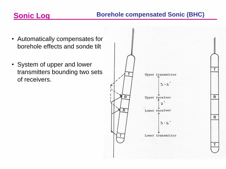
Sonic Log

• Automatically compensates for

borehole effects and sonde tilt

• System of upper and lower

transmitters bounding two sets

of receivers.

Borehole compensated Sonic (BHC)

Sonic Log Comparison of BHC with Basic Sonic

Sonic Log

Wyllie Eq. - linear time averaged relationship

– empirically determined

– for clean and consolidated sandstones

– uniformly distributed small pores

Porosity

maV

L

maL

fV

L

fL

t

Sonic Log Porosity

mat

ft

mat

logt

Wyllie Equation

tma,msec/ft tf,msec/ft

ss 55.5 fresh 189

lms 47.6 salt 185

dol 43.5

Anhy 50.0

Sonic Log

Evidence: when tlog > 100 microsec/ft in overlying shale

Result: Estimated porosity too high

Correction: Observed transit times are greater in uncompacted sands;

thus apply empirical correction factor, Cp

Estimate Cp from overlying shale zone

where the shale compaction coefficient, c , ranges from 0.8 < c < 1.3.

Porosity – uncompacted sands

pC

1

mat

ft

mat

logt

100

sht

cp

C

Sonic Log

• Sonic primarily independent of fluid type

• Know lithology, can calculate porosity

• Fluid Effect in high porosity formations with high HC saturation.

Correct by:

• Apply after compaction correction.

Porosity – uncompacted sands-Fluid Effect

s*7.0

corr :gas

s*9.0

corr :oil

Sonic Log Example

31%

34%

32%

33%

Ave zone

Core Cp = 1.44…from overlying shale

Sonic Log

Transit time - porosity transform (Raymer-Hunt)

– based on field observation

– yields slightly greater porosity in the 5 to 25% range

– does not require compaction correction

Where

C ranges from 0.625 to 0.700

Typical value used in practice is C = 0.67

C = 0.6 for gas-saturated formations

Porosity

logt

mat

logt

C

tma, msec/ft

Ss 56.0

Lms 49.0

Dolo 44.0

Sonic Log Porosity comparison

Sonic Log

– Sonic ignores secondary

porosity; i.e, vugs and fractures

– Result: Measured transit time <

than would be calculated for

given porosity

– Estimate Secondary porosity

by:

– Alternative: Develop specific

empirical relationships for

heterogeneous systems

Secondary Porosity

st

2

Example of Porosity – Velocity Correlation in Dolomite

The example illustrates travel times which are

consistently greater than predicted by the

“time-average equation”. (Corelab)

Sonic Log

Theory, Measurement, and Interpretation of Well Logs, Bassiouni, SPE

Textbook Series, Vol. 4, (1994)

Chapter 3 – Acoustic Properties of Rocks

Chapter 10 – Sonic Porosity Log

• Schlumberger, Log Interpretation Charts, Houston, TX (1995)

• Schlumberger, Log Interpretation and Principles, Houston, TX (1989)

• Western Atlas, Log Interpretation Charts, Houston, TX (1992)

• Western Atlas, Introduction to Wireline Log Analysis, Houston, TX (1995)

• Halliburton, Openhole Log Analysis and Formation Evaluation, Houston, TX (1991)

• Halliburton, Log Interpretation Charts, Houston, TX (1991)

References