Chapter 12Multimodel-Inference in ComparativeAnalyses

László Zsolt Garamszegi and Roger Mundry

Abstract Multimodel inference refers to the task of making a generalization fromseveral statistical models that correspond to different biological hypotheses andthat vary in the degree of how well they fit the data at hand. Several approacheshave been developed for such purpose, and these are widely used, mostly forintraspecific data, i.e., in a non-phylogenetic framework, to draw inference frommodels that consider different predictor variables in different combinations.Adding the phylogenetic component, in theory, calls for a more extendedexploitation of these techniques as several hypotheses about the phylogenetichistory of species and about the mode of evolution should also be considered, all ofwhich can be flexibly incorporated and combined with different statistical models.Here, we highlight some biological problems that inherently imply multimodelapproaches and show how these problems can be tackled in the phylogeneticgeneralized least squares (PGLS) modeling framework based on information-theoretic approaches (e.g., by using Akaike’s information criterion, AIC) ormaximum likelihood. We present a conceptual framework of model selection forphylogenetic comparative analyses, where the goal is to generalize across modelsthat involve different combinations of predictors, phylogenetic hypotheses,parameters describing the mode of evolution, and error structures. Although thisoverview suggests that a model selection strategy may be useful in several situ-ations, we note that the performance of the approach in the phylogenetic contextawaits further evaluation in simulation studies.

L. Z. Garamszegi (&)Department of Evolutionary Ecology, Estación Biológica de Doñana-CSIC,Seville, Spaine-mail: laszlo.garamszegi@ebd.csic.es

R. MundryMax Planck Institute for Evolutionary Anthropology, Leipzig, Germanye-mail: roger_mundry@eva.mpg.de

L. Z. Garamszegi (ed.), Modern Phylogenetic Comparative Methods and TheirApplication in Evolutionary Biology, DOI: 10.1007/978-3-662-43550-2_12,� Springer-Verlag Berlin Heidelberg 2014

305

12.1 Introduction

The world is so complex that researchers are often confronted with the challenge ofassessing a large number of biological explanations for a given phenomenon(Chamberlin 1890). Making drawing inference from multiple hypotheses tradi-tionally involves the evaluation of the appropriateness of different statistical modelsthat describe the relationship among the considered variables. This task can be seenas a model selection problem, and there are three general approaches that allow suchinference based on statistical analysis. The approach that dominated applied sta-tistics for decades is that of null-hypothesis significance testing (NHST)(Cohen 1994). Applying NHST, one typically states a null-hypothesis of no influ-ence or no difference, which is then rejected or not based on a significance threshold(conventionally, P = 0.05 that specifies the probability that one would obtain theobserved data given the null hypothesis were true). In this framework, nestedmultiple models can be examined in a stepwise fashion, in which terms can beeliminated or added based on their significance following a backward or forwardprocess (but see, e.g., Mundry and Nunn 2008; Whittingham et al. 2006; Hegyi andGaramszegi 2011 for problems with stepwise model selection). The secondapproach is Bayesian inference where one considers a range of ‘hypotheses’ (e.g.,model parameters) and incorporates some prior knowledge about the probability ofthe particular model parameter values to update one’s ‘belief’ in what are more andless likely model parameters (Congdon 2003; Gamerman and Lopes 2006).Bayesian inference has a long history, but only recent increases in computer powermade its application feasible for a wide range of problems (for relevance forcomparative studies, see Chaps. 10 and 11). The third, relatively recent approach tostatistical inference is based on information theory (IT) (Burnham andAnderson 2002; Johnson and Omland 2004; Stephens et al. 2005). Here, a set ofcandidate models, which represent different hypotheses, is compared with regard tohow well they fit the data. A key component of the IT approach is that the measureof model fit is penalized for model complexity (i.e., the number of estimatedparameters), and, as such, IT-based inference aims at identifying models that rep-resent a good compromise between model fit and model complexity. Most fre-quently, IT-based inference goes beyond simply choosing the best model (out of theset of candidate models) and allows accounting for model selection uncertainty (i.e.,the possibility that several models receive similar levels of support from the data).

Although model selection is classically viewed as a solution to the problemcaused by the large number of potential combinations of predictors that may affectthe response variable, here we propose that the comparative phylogenetic frameworkinvolves a range of questions that require multimodel inference and approachesbased on IT. In particular, we emphasize that in addition to the variables included inthe candidate models, the models can also differ in terms of other parameters thatdescribe the mode of evolution, or account for phylogenetic uncertainty and heter-ogeneities in sampling effort. In this chapter, we present general strategies fordrawing inference from multiple evolutionary models in the framework of

306 L. Z. Garamszegi and R. Mundry

phylogenetic generalized least squares (PGLS). We formulate our suggestionsmerely on a conceptual basis with the hope that these will stimulate further researchthat will assess the performance of the methods based on simulations. We envisagethat such simulation studies are crucial steps before implementing model selectionroutines into the practice of phylogenetic modeling. Our discussion is accompaniedwith an Online Practical Material (hereafter OPM) available at http://www.mpcm-evolution.org, which demonstrates how our methodology can be applied toreal data in the R statistical environment (R Development Core Team 2013).

12.2 The Fundaments of IT-based Multimodel Inference

Given that a considerable number of primary and secondary resources discuss thedetails of the IT-based approach (Burnham and Anderson 2002; Claeskens andHjort 2008; Garamszegi 2011; Konishi and Kitagawa 2008; Massart 2007), weavoid giving an exhausting description here. However, in order to make oursubsequent arguments comprehensible for the general readership, we first providea brief overview on the most important aspects of the approach.

12.2.1 Model Fit

The central idea of an IT-based analysis is to compare the fit of different models inthe candidate model set (see below). However, it is trivial that more complexmodels show better fits (e.g., larger R2 or smaller deviance). Hence, an IT-basedanalysis aims at identifying those models (in the set of candidate models; seebelow) that represent a good compromise between model complexity and modelfit, in other words, parsimonious models. Practically, this is achieved by penalizingthe fit of the models by their complexity. One way of doing this is to use Akaike’sinformation criterion (AIC), namely

AIC ¼ �2 lnL modeljdatað Þ þ 2k; ð12:1Þ

whereL modeljdatað Þ maximum likelihood of the model given the data and the parameter

estimates,k the number of parameters in the model (�2 lnL modeljdatað Þ is known

as ‘‘deviance’’).

Two models explaining the data equally well will have the same likelihood, butthey might differ in the number of parameters estimated. Then, the model with thesmaller number of parameters will reveal the smaller AIC (and the difference inthe AIC values of the more complex and the simpler model will be twice the

12 Multimodel-Inference in Comparative Analyses 307

difference of the numbers of parameters they estimate). Hence, in an IT-basedanalysis, the model with the smaller AIC is considered to be ‘better’ because itrepresents a more parsimonious explanation of the response investigated.1 Note-worthy, some argue that AIC-based inference can select for overly complexmodels and suggest alternative information criteria (Link and Barker 2006). Here,we continue focusing on AIC with the notion that the framework can be easilytailored for other metrics.

The core result of an IT-based analysis is a set of AIC values associated with aset of candidate models. However, unlike P values, AIC values do not have aninterpretation in themselves but receive meaning only by comparison with AICvalues of other models, fitted to the exact same response. The model with thesmallest AIC is the ‘best’ (i.e., best compromise between model parsimony andcomplexity) in the set of models. However, in contrast to an NHST analysis, itwould be misleading to simply select the best model and discard the others. This isbecause the best model according to AIC (i.e., the one with the smallest AIC)might not be the model that explicitly describes the truth (in fact, it is unlikely toever be). Such discrepancies can happen for various reasons, including stochas-ticity in the sampling process (i.e., a sample is used to draw inference about apopulation), measurement error in the predictors and/or the response, or unknownpredictors not being in the model, to mention just a few. An analysis in theframework of a phylogenetic comparative analysis expands this list considerablyto include, for instance, imperfect knowledge about the phylogenetic history or theunderlying model of evolution (e.g., Brownian motion or Ornstein-Uhlenbeck). AnIT-based analysis allows dealing elegantly with such model selection uncertaintyby explicitly taking it into account (see below).

12.2.2 Candidate Model Set

A key component in an IT-based analysis is the candidate set of models to beinvestigated, which classically includes models with different combinations ofpredictors. The validity of the analysis is conditional on this set, and if the can-didate model set is not a reasonable one, the results will be deceiving (Burnhamand Anderson 2002; Burnham et al. 2011). Hence, the development of the can-didate set needs much care and is a crucial and potentially challenging step of anIT-based analysis. First of all, different models might represent different researchhypotheses. For instance, one might hypothesize that brain size might have co-evolved with social complexity (e.g., group size), ecological complexity (e.g.,seasonality in food availability), or both. However, in biology, it is frequently noteasy to come up with such a clearly defined set of potentially competing models,

1 When drawing inference in an IT framework, it is essential to not mix it up with the NHSTframework. Most crucially, it does not make sense to select the best model based on AIC and thentest its significance or the significance of the predictors it includes.

308 L. Z. Garamszegi and R. Mundry

and hence one frequently sees candidate model sets that encompass all possiblemodels that can be built out of a set of predictors. Furthermore, in the context ofphylogenetic comparative analysis, different models in the candidate set mightrepresent different evolutionary models (e.g., Brownian motion or an Ornstein-Uhlenbeck process) or different phylogenies. It is important to emphasize that in aphylogenetic comparative analysis both these aspects (and also other ones) can bereflected in a single candidate set of models; that is, the candidate set mightcomprise models that represent combinations of hypotheses about the coevolutionof traits, the model of evolution, and the phylogenetic history.

12.2.3 Accounting for Model Uncertainty

There are several ways of dealing with model selection uncertainty (i.e., with thefact that not only one model is unanimously selected as best). One way is toconsider Akaike weights. Akaike weights are calculated for each model in the setand can be thought of as the probability of the actual model to be the best in the setof models (although there are warnings against such interpretations, e.g., seeBolker 2007). From Akaike weights, one can also derive the evidence ratio of twomodels, which is the quotient of their Akaike weights and tells how much morelikely is one of the two models (i.e., the one in the numerator of the evidence ratio)to be the best model. Akaike weights can also be used to infer about the impor-tance of individual predictors by summing Akaike weights for all models thatcontain a given predictor. The summed Akaike weight for a given predictor thencan be considered analogous to the probability of it being in the best model of theset (see also Burnham et al. 2011; Symonds and Moussalli 2011).

12.2.3.1 Model Averaging

One can also use Akaike weights for model averaging of the estimated coefficientsassociated with the different predictors. Here, the estimated coefficients (e.g.,regression slopes) are averaged across all models (or across a confidence set of bestmodels2) weighted by the Akaike weights of the corresponding models (see alsoBurnham et al. 2011; Symonds and Moussalli 2011). Hence, an estimate of acoefficient from a model having a large Akaike weight contributes more to the

2 Another way of dealing with model selection uncertainty is to consider the best modelconfidence set, which contains the models that can be considered as best with some certainty.Different criteria do exist to identify the best model confidence set among which the most popularare to include those models that differ in AIC from the best model by at most some threshold(e.g., 2 or 10) or, alternatively, to include those models for which their summed cumulativeAkaike weights (from largest to smallest) just exceed 0.95. In this chapter, we do not considersuch subjective thresholds further, and throughout the remaining discussion we refer to modelaveraging in a sense that it is made across the full model set.

12 Multimodel-Inference in Comparative Analyses 309

averaged value of the coefficient. When using model averaging of the estimatedcoefficients, there are two ways of treating models in which a given predictor is notpresent: one is to simply ignore them (the ‘natural’ method), and one is to set theestimated coefficient to zero for models in which the given predictor is not included(the ‘zero’ method; Burnham and Anderson 2002; Nakagawa and Hauber 2011).Using the latter penalizes the estimated coefficient when it is mainly included inmodels with low Akaike weights, and to us, this seems to be the better method.

12.3 Model Selection Problems in PhylogeneticComparative Analyses

There can be several biological questions involving phylogenies, which necessitateinference from more than one model that are equally plausible hypothetically.Most readers might have encountered such a challenge when judging the impor-tance of different combinations of predictor variables. However, in addition toparameters that estimate the effects of different predictors, in a phylogeneticmodel, there are several other parameters that deal with the role of phylogenetichistory or with another error term (e.g., within-species variance). The statisticalmodeling of these additional parameters often requires multiple models that dif-ferently combine them, even at the same set of predictors. Below, we demonstratethat in most of these situations the observer is left with the classical problem ofmodel selection, when s/he needs to draw inferences from a pool of models basedon their fit to the data. Accordingly, the same general framework can be applied:Competing biological questions are first translated into statistical models, and then,multimodel inference is used for generalization.

12.3.1 Selecting Among Evolutionary Models with DifferentCombinations of Predictors

The classical problem of finding the most plausible combination of predictors toexplain interspecific variation in the response variable while accounting for thephylogeny of species is well exemplified in the comparative literature. Startingfrom a pioneering study by Legendre et al. (1994), a good number of studies existthat evaluate multiple competing models to assess their relative explanatory valueand to draw inferences about the effects of particular predictors. Below, as anappetizer, we provide summaries of two of these studies to demonstrate thediversity of questions that can be addressed by using the model selection frame-work. In the OPM, we give the R code that can be easily tailored to any biologicalproblem requiring an AIC-based information-theoretic approach.

Terribile et al. (2009) investigated the role of four environmental hypothesesmediating interspecific variation in body size in two snake clades. These hypotheses

310 L. Z. Garamszegi and R. Mundry

emphasized the role of heat balance as given by the surface area-to-volume ratio,which in ectothermic vertebrates may influence heat conservation (e.g., small-bodied animals may benefit from rapid heating in cooler climates), habitat avail-ability (habitat zonation across mountains limits habitat areas that ultimately selectfor smaller species), primary productivity (low food availability can reduce growthrate and delay sexual maturity, which would in turn result in small-bodied species inareas with low productivity), and seasonality (large-bodied species may be moreefficient in adapting to seasonally fluctuating resources that often include periods ofstarvation). To test among these hypotheses, the authors estimated the extent towhich the patterns of body size are driven by current environmental conditions asreflected by mean annual temperature, annual precipitation, primary productivity,and range in elevation. They challenged a large number of models with data andchose the best model that offered the highest fit relative to model complexity todraw inference about the relative importance of different hypotheses. This bestmodel included all main predictors, but the amount of variation explained differedbetween Viperidae and Elapidae, the two snake clades investigated. Moreover, therelative importance for each predictor also varied, as indicated by the summedAkaike weights. Consequently, none of the proposed hypotheses was over-whelmingly supported or could be rejected, and the mechanisms constraining bodysize in snakes can even vary from one taxonomic group to another.

A recent phylogenetic comparative analysis of mammals focused on thedeterminants of dispersal distance, a variable of major importance for manyecological and evolutionary processes (Whitmee and Orme 2013). Dispersal dis-tance can be hypothesized as a trait being influenced by several constraints arisingfrom life history, a situation that necessitates multipredictor approaches. Forexample, larger body size can allow longer dispersal distances because locomotionis energetically less demanding for larger-bodied animals. Second, home rangesize may be important, as dispersing individuals of species using larger homeranges may need to move longer distances to find empty territories. Furthermore,trophic level, reflecting the distribution of resources, may mediate dispersal dis-tance with carnivores requiring more dispersed resources than herbivores oromnivores. Intraspecific competition may also affect dispersal: species maintaininghigher local densities may also show higher frequencies of distantly dispersingindividuals which thereby encounter less competition. Finally, investment inparental activities can be predicted to negatively influence dispersal, as species thatwean late and mature slowly will create less competitive conditions for theiroffspring than species with fast reproduction. To simultaneously evaluate theplausibility of these predictors, Whitmee and Orme (2013) applied a modelselection strategy based on the evaluation of a large number of models composedof the different combinations (including their quadratic terms) of the consideredpredictors. Even the best-supported multipredictor models had low Akaikeweights, indicating no overwhelming support for any particular model. Therefore,they applied model averaging to determine the explanatory role of particularvariables, which indicated that home range size, geographic range size, and bodymass are the most important terms across models.

12 Multimodel-Inference in Comparative Analyses 311

12.3.2 Dealing with Phylogenetic Uncertainty: InferenceAcross Models Considering Different PhylogeneticHypotheses

While phylogenetic comparative studies necessarily require a phylogenetic tree,the true phylogeny is never known and must be estimated from morphological or,more recently, from genetic data; thus, phylogenies always contain some uncer-tainty (see detailed discussion in Chap. 2). In several cases, more than one phy-logenetic hypothesis (i.e., tree) can be envisaged for a given set of species, and itmight be desirable to test whether the results found for a given phylogenetic treeare also apparent for other, similarly likely trees.

With GenBank data and nucleotide sequences for phylogenetic inference, theabove problem is not restricted anymore to the comparison of a handful of alter-native trees corresponding to different markers. Nonetheless, the reconstruction ofphylogenies from the same molecular data still raises uncertainty issues at severallevels. Different substitution models and multiple mechanisms can be considered forsequence evolution, each leading to different sets of phylogenies that can be con-sidered (note that this is also a model selection problem). Moreover, even the samesubstitution model can lead to various phylogenetic hypotheses with similar like-lihoods. As a result, in the recent day’s routine, several hundreds or even thousandsof phylogenetic trees are often available for the same list of species used in acomparative study. The most common way to deal with such a large sample of treesis the use of a single, consensus tree in the phylogenetic analysis. However, althoughthis approximation is convenient from a practical perspective, using an ‘average’tree does not capture the essence of uncertainty, which lies in the variation across thetrees. The whole sample of similarly likely trees defines a confidence range aroundthe phylogenetic hypothesis (de Villemereuil et al. 2012; Pagel et al. 2004).

For the appropriate treatment of phylogenetic uncertainty, one needs to incor-porate an error component that is embedded in the pool of trees that can beenvisaged for the species at hand. Martins and Hansen (1997) proposed that mostquestions in relation to the evolution of phenotypic traits across species can betranslated into the same general linear model:

y ¼ bXþ e; ð12:2Þ

wherey is a vector of characters or functions of character states for extant or ancestral

taxa,X is a matrix of states of other characters, environmental variables, phylogenetic

distances, or a combination of these,b is a vector of regression slopes,e is a vector of error terms with an assumed structure.

312 L. Z. Garamszegi and R. Mundry

e is composed of at least three types of errors that can be assembled in acomplex way: eS; the error due to common ancestry; eM; the error due to within-species variance or measurement error; and eP; the error due phylogenetic uncer-tainty. The regression technique based on PGLS when combined with maximumlikelihood (ML) model fitting offers a flexible way to handle and combine theerrors eS and eM (for example, they can be treated additively if they are inde-pendent, see Chaps. 5 and 7). However, simultaneously handling the third error,the one that is caused by phylogenetic uncertainty, eP; is more challenging, becauseit is not an independent and additive term (Martins 1996). Approaches based onBayesian sampling that are discussed in Chap. 10 offer a potential solution. Theyallow the use of a large number of similarly likely phylogenetic trees by effectivelyweighting parameter estimates across their probability distribution and can alsoincorporate errors due to within-species variance (de Villemereuil et al. 2012).However, widely available Bayesian methods can be sensitive to prior settings andare not yet implemented in the commonly used statistical packages.

We propose a simpler solution and suggest that when combined with multi-model inference, approaches based on PGLS can be used to deal with uncertaintiesin the phylogenetic hypothesis. The underlying philosophy of this approach is thatwhen a list of trees is available, each of them can be used to fit the same modeldescribing the relationship between traits using ML. Subsequently, parameterestimates (e.g., intercepts and slopes) can be obtained from the resulting models,which can then be averaged with a weight that is proportional to the relative fit ofthe corresponding model to the data. The output will not only provide a singleaverage effect (as is the case when using a single model fitted to a consensus tree)but will also include a confidence or error range as obtained from the variance ofmodel parameters across models associated with different trees. This interval canbe interpreted as a consequence of the uncertainty in the phylogenetic hypothesis,that is, the mean estimate (model-averaged slope, or the slope that is based on theconsensus tree) with the associated uncertainty component (variance among par-ticular slopes) will form the results together. The logic of analyzing the inter-specific data on each possible phylogeny to obtain a sample of estimates and thento calculate summary statistics from this distribution was already proposed byMartins (1996). Our favored method differs with regard to that it applies a model-averaging technique to derive the mean and confidence interval from the frequencydistribution of parameters. This can be important, because if the pool of the treesacross which the models are fitted reflects the likelihood of particular treesexplaining the evolution of taxa, the resulting model-averaged parameter estimateswill also reflect this variation.

Although apparently different trees are used in each model, drawing inferenceacross them does not violate the fundaments of information theory that assumesthat each model is fitted to the very same data. Different trees can be regarded asdifferent hypotheses that arise from identical nucleotide sequence information.They are actually just different statistical translations of the same biologicalinformation and act like scaling parameters on the tree. The approach may beparticularly useful when a large number of alternative trees are at hand (e.g., in the

12 Multimodel-Inference in Comparative Analyses 313

form of a Bayesian sample originating from the same sequence data). When only ahandful of phylogenies is available (e.g., from other published papers), model-averaged means and variances can also be calculated, but conclusions would beconditional on the phylogenies considered (i.e., some alternative phylogenies mayhave not been evaluated). Furthermore, fitting models to trees that correspond todifferent marker genes calls for philosophical issues about the underlyingassumption concerning the use of the same data.

In Fig. 12.1, we illustrate how our proposed model averaging works in practice(the underlying computer codes are available in the OPM). In this example, wetested for the evolutionary relationship between brain size and body size in primatesby using PGLS regression methods with ML estimation of parameters. We con-sidered a sample of reasonable phylogenetic hypotheses in the form of 1,000 trees asobtained from the 10KTrees Project (Arnold et al. 2010). When using the consensustree from this tree sample, we can estimate that the phylogenetically correctedallometric slope is 0.287 (SE = 0.039, solid line in Fig. 12.1). However, usingdifferent trees from 10KTrees pool in the model provides slightly different results forthe phylogenetic relationship between traits, as the obtained slopes vary (gray linesin the left panel of Fig. 12.1). The model-averaged regression slope yields 0.292(model-averaged SE = 0.041, dashed line in the left panel of Fig. 12.1). This meanestimate is quite close to what one can obtain based on the consensus tree, but thevariation between the particular slopes corresponding to different trees in the sampledelineates some uncertainty around the averaged allometric coefficient. Few modelsin the ML sample provide extreme estimates (note that, model fitting with oneparticular tree even results in a negative slope, left panel of Fig. 12.1). However,these models were characterized by a very poor model fit; thus, their potentialinfluence is downweighted in the model-averaged mean estimate.

The benefit of using the AIC-based method to account for phylogenetic uncer-tainty over Bayesian approaches is that the former does not require prior informationon model parameters that would affect the posterior distribution of parameters, anissue that is often challenging in the Bayesian framework (Congdon 2006) and thatis also demonstrated in Fig. 12.1. In the right panel, we applied Markov chain MonteCarlo (MCMC) procedure to estimate the posterior distribution of parameter valuesfrom the same PGLS equation by using (Pagel et al. 2004; Pagel and Meade 2006)BayesTraits with the same interspecific data and pool of trees (see also Chap. 10).Supposing that we have no information to make an expectation about the rangewhere parameter estimates should fall, we are constrained to use flat and uniformprior distributions (e.g., spanning from -100 to 100).3 When we used MCMC to

3 It may not be necessarily applied to the current biological example, because allometricregressions are intensively studied (e.g., Bennett and Harvey 1985; Hutcheon et al. 2002; Iwaniuket al. 2004; Garamszegi et al. 2002). Therefore, results from a large number of studies on othervertebrate taxa may be used to define a narrower and more informative prior. However, in thisexample simulated on the general situation when no preceding information on the expectedrelationship is available. Note that technically BayesTraits only allows uniform priors forcontinuous data.

314 L. Z. Garamszegi and R. Mundry

sample from a large number of models with different parameters and trees and took1,000 estimates from the posterior distribution of slopes, we detected that theestimate is accompanied by a considerable uncertainty (Fig. 12.1, right panel). Forcomparison, the 95 % confidence interval of the allometric coefficients obtainedfrom the ML sample is 0.278–0.312, while it is 0.211–0.373 for the MCMC sample(i.e. the confidence interval obtained from the Bayesian framework is almost fivetimes wider than that from the AIC-based inference). Consequently, the Bayesianapproach introduces an unnecessary uncertainty due to the dominance of the priordistribution on the posterior distribution.

Another benefit of using ML model fitting over a range of phylogenetichypotheses in conjunction with model averaging is that by doing so we can exploitthe flexibility of the PGLS framework. For example, as we discussed above, onecan evaluate different sets of predictor variables when defining models, or as weexplain below, one can also take into account additional error structures (e.g., dueto within-species variation) or different models of trait evolution (e.g., Brownianmotion or an Ornstein-Uhlenbeck process). These different scenarios can besimultaneously considered during model definition, but can also be combined with

4 6 8 10

12

34

56

7

log(Body size)

log(

Bra

in s

ize)

4 6 8 10

12

34

56

7

log(Body size)

log(

Bra

in s

ize)

Fig. 12.1 Estimated regression lines for the correlated evolution of two traits (body size andbrain size in primates) when different hypotheses for the phylogenetic relationships of species areconsidered and when ML (left panel) or MCMC (right panel) estimation methods are used in theAIC-based or Bayesian framework, respectively. Gray lines show the regression slopes that canbe obtained for alternative phylogenetic trees (left panel 1,000 ML models fitted to different trees,right panel 1,000 models that the MCMC visited in the Bayesian framework). The alternativetrees originate from a sample of 1,000 similarly likely trees that can be proposed for the samenucleotide sequence data (Arnold et al. 2010). The dashed bold line represents the slope estimatethat can be derived by model averaging over the particular ML estimates (left panel) or by takingthe mean of the posterior distribution from the MCMC sample of 1,000 models (right panel).Both methods provide a mean estimate over the entire pool of trees by incorporating theuncertainty in the underlying phylogenetic hypothesis. The solid bold line shows the regressionline that can be fitted when the single consensus tree is used. The model-averaged slope, the meanof the posterior distribution, and the one that corresponds to the consensus highly overlap in thisexample (which may not necessarily be the case). However, the precision by which the mean canbe estimated is different between ML and MCMC approaches, as the latter introduces a largervariance in the slopes in the posterior sample

12 Multimodel-Inference in Comparative Analyses 315

alternative phylogenetic trees (some examples are given in the OPM). This willresult in a large number of candidate models representing different evolutionaryhypotheses, over which model averaging may offer interpretable inference.

Box 12.1 A simulation strategy for testing the performanceof multimodel inference

The behaviour of the AIC-based framework to account for phylogeneticuncertainty requires simulation studies that consist of the following steps.First, one needs to simulate a tree for a considered number of species andunder some scenario for the underlying model (e.g., time-dependent birth–death model or just a random tree). The next step is then to simulate species-specific trait data along the branches of the generated phylogeny. To obtainsimulated tip values, we also need to consider a model to describe theevolutionary mechanism in effect (e.g., Brownian motion or an OU process).We might also consider other constraints for trait evolution, for example, bydefining a correlation structure (a zero or a nonzero covariance) for twocoevolving traits. These parameters will serve as generating values, and theunderlying tree and the considered covariance structure will reflect the truththat we want to recover in the simulation. If the interest is to examine theperformance of the model-averaging strategy to account for phylogeneticuncertainty, we need to generate a sample of trees that integrates a givenamount of variance (e.g., both the topology and branch lengths are allowedto vary to some pre-defined degree). For each simulation, we can then fit amodel estimating the association between the two traits by controlling forphylogenetic effects. The phylogeny used in this model to define theexpected variance–covariance structure on the one hand can be the con-sensus tree calculated for the whole sample of trees. On the other hand, wecan also fit the model to each tree in the sample and then do a modelaveraging to obtain an overall estimate for the parameter of interest (e.g.,slope or correlation as calculated from the model). By simulating new traitdata (and optionally new pools of trees), we can repeat the whole process alarge number of times (i.e., 1,000 or 10,000 times). At each iteration, wewill, hence, obtain estimates (either over the consensus tree or over the entiresample of trees through model averaging) for the parameter of interest.Finally, we can compare the distribution of these parameters over simula-tions with the generating parameter state. The difference between the meanof the distribution and the generating value will inform about bias of theapproach, while the width of the distribution informs about precision (theuncertainty in parameter estimation).

As an important cautionary note, we emphasize that the performance of theAIC-based method based on model averaging still requires further assessment withboth simulated and empirical data. In Box 12.1, we describe the philosophy of an

316 L. Z. Garamszegi and R. Mundry

appropriate simulation study that can efficiently test the performance of averagingparameters over a large number of models corresponding to different hypothesesabout phylogenies or other evolutionary patterns.

12.3.3 Variation Within Species

One of the advantages of the PGLS approach is that it allows accounting forwithin-species variation, which broadly includes true individual-to-individual orpopulation-to-population variation, and also other sources of variation in theestimates of taxon trait values such as measurement error (see Ives et al. 2007;Hansen and Bartoszek 2012; and Chap. 7). Given that these different sources oferror can be translated into different models, selecting among these may also beperformed by model selection. Does a model that considers within-species vari-ation perform better than a model that neglects such variation? Such simplequestions can be developed further as by applying the general Eq. 12.2, in whichdifferent error structures (e.g., phylogenetic errors and measurement errors, ormeasurement error on one trait may correlate with measurement error on anothertrait) can be combined in different ways.

For example, when considering intraspecific variation in an interspecific con-text, we can evaluate at least four models and compare them based on their relativefit (here, we are only focusing on the main logic; for details on how to take intoaccount intraspecific variation, see Chap. 7). First, as a null model, we can fit amodel that is defined as an ordinary least squares regression (i.e., with a covariancematrix for the residuals based on a star phylogeny and measurement errors beingzero). Then, we can investigate a model that does account for phylogeny but notfor the uncertainty in the species-specific trait values (conditioned on the truephylogeny, while measurement errors are assumed to be equal to zero), and also amodel that considers measurement error but ignores the phylogenetic structure(unequal and nonzero values along the diagonal of the measurement error matrix,and a phylogenetic covariance matrix representing a star phylogeny). Finally, wewish to test a model that includes both error structures (the joint vari-ance–covariance matrix reflecting the phylogeny and the known measurementerrors). To obtain parameter estimates and to make appropriate evolutionaryconclusions, the observer can rely on the model that offers the best fit to the data asindicated by the corresponding AIC (but only if one model is unanimously sup-ported over the others). Such a simple model selection strategy can be followed inthe OPM of Chap. 7. Note that for the appropriate calculation of AIC according toEq. 12.1 (and thus for the meaningful comparison of models), it is required that thenumber of estimated parameters is determined, which may be difficult whenparameters in both the mean and variance components are estimated. This problemcan be avoided by a smart definition of models (e.g., by defining analog modelsthat estimate the same number of parameters even if these are known to be zero).In any case, the approach requires further validation by simulation studies.

12 Multimodel-Inference in Comparative Analyses 317

Methods that account for within-species variation can also deal with a situation,in which different sample sizes (n) are available for different species, implying thatdata quality might be heterogeneous (i.e., larger errors in taxa with lower samplingeffort; see Chap. 7 for more details). For example, if within-species variances orstandard errors are unknown, one can fit a measurement error model by using1/n as an approximation of within-species variance.

Another way to incorporate heterogeneous sampling effort across species intothe comparative analyses is to apply statistical weights in the model. A particularissue arising in this case is that weighting can result in a large number of models(with potentially different results). For example, by using the number of individ-uals sampled per taxon as statistical weights in the analysis, we enforce weightsdiffering a lot between species that are already sampled with sufficient intensity(e.g., the underlying sample size is 20 at least) but still differ in the backgroundresearch effort (e.g., 100 individuals are available for one species, while 1,000 foranother). However, if we log- or square-root-transform within-species sample sizesand use these as weights, more emphasis will be given on differences betweenlightly sampled species than on differences between heavily sampled species.Continuing this logic, and applying the appropriate transformation, we can create afull gradient that scales differences in within-species sample sizes along a con-tinuum spanning from no differences to large differences between species withdifferent within-species sample sizes.

For illustrative purposes (Fig. 12.2, left panel), we have created such a gradientof statistical weights by the combination of the original species-specific samplesizes (n) and an emphasis parameter (the ‘weight of weights’) that we will label x;x is simply an elevation factor that ranges from 1 to 1/100 and defines theexponent of n. If x is 1, the original sample sizes are used as weights in theanalysis. If x is 1/2 = 0.5, the square-root-transformed values serve as weights,and differences between small sample sizes become more emphasized than dif-ferences between species with larger sample sizes. x = 1/? = 0 represents thescenario in which all species are considered with equal weight (n0 = 1), so themodel actually represents a model that does not take into account heterogeneity insampling effort. Other transformations on sample sizes based on different scalingfactors that create a gradient can also be envisaged.

Using the parameter x, we provide an example for the study of brain sizeevolution based on the allometric relationship with body size (Fig. 12.2 rightpanel, the associated R code is provided in the OPM). We have created a set ofphylogenetic models that also included statistical weights in the form of the xexponent of within-species sample sizes. The scaling factor x varied from 0 to 1.We challenged these models with exactly the same data using ML; thus, model fitstatistics (e.g., AIC) are comparable. We found that when accounting for phylo-genetic relationships, the x = 0 scenario provides by far the best fit, implying thatweighting species based on sample size is not important. This finding is notsurprising, given that both traits, brain size and body size, have very highrepeatability (R [ 0.8). Thus, relatively few individuals provide reliable infor-mation on the species-specific trait values. Giving different weights to different

318 L. Z. Garamszegi and R. Mundry

species based on the underlying sample sizes would actually be misleading; the useof different x values leads to qualitatively different parameter estimates for theslope of interest (Fig. 12.2, right panel). This indicates that the results and con-clusions are highly sensitive to how differences in sampling effort are treated in theanalysis. Note that the above exercise only makes sense if (1) there is a consid-erable variation in within-species sample size and (2) if there is no phylogeneticsignal in sample sizes. These assumptions require some diagnostics prior to thecore phylogenetic analysis (see an example in Garamszegi and Møller 2012).

Garamszegi and Møller (2007) relied on a similar approach in a study of theecological determinants of the prevalence of the low pathogenic subtypes of avianinfluenza in a phylogenetic comparative context. It was evident that there was avast variance in sampling effort across species, as within-species sample sizevaried between 107 and 15,657. Therefore, when assessing the importance of theconsidered predictors, it seemed unavoidable to simultaneously account forcommon ancestry and heterogeneity in data quality. The application of the strategyof scaling the weight factor yielded that, contrary to the above example, thehighest ML was achieved by a certain combination of the weight and phylogeneticscaling parameters. That finding was probably driven by the relatively modestrepeatability of the focal trait (prevalence of avian influenza), suggesting that, dueto different sample sizes, data quality truly differed among species.

We advocate that the importance of a correction for sample size differencesbetween species is an empirical issue that can vary from data to data, which could(and should) be evaluated. We provided a strategy by which the optimal scaling ofweight factors can be determined. In these examples, an unambiguous support could

0 20 40 60 80 100

0

20

40

60

80

100

Within-species sample size (n)

Wei

ghts

use

d in

the

anal

ysis

(nom

ega ) n

n0.9

n0.7

n0.5

n0.1

0.0 0.2 0.4 0.6 0.8 1.0

-70

-60

-50

-40

-30

omega

Max

imum

log-

likel

ihoo

d

0.0

0.2

0.4

0.6

0.8

1.0

slop

e

Fig. 12.2 The effect of using different transformations of the number of individuals as statisticalweights. The left panel shows how differences between species are scaled when the underlyingwithin-species sample sizes are transformed by exponentiating them with the exponent x. xvaried between 1 (untransformed sample sizes maximally emphasizing differences in data qualitybetween species) and 0 (all species have the same weight; thus, data quality is considered to behomogeneous). The right panel shows the maximized log-likelihood (black solid line) and theestimated slope parameters of models (red dashed line) for the brain size/body size evolution thatimplement weights that are differently scaled by x

12 Multimodel-Inference in Comparative Analyses 319

be obtained for a single parameter combination. However, we can imagine situa-tions, in which more than one model offers relatively good fit to the data, in whichcase inference would be better made based on model averaging (correspondingcodes are given in the OPM) instead of focusing on a single parameter combination.Furthermore, the evaluation of the sample size scaling factor (as well as theassessment of within-species variance) can be combined with the evaluation ofalternative phylogenetic hypotheses, as the IT-based framework offers a potentialfor the exploration of a multidimensional parameter space. Accordingly, eachscaling factor can be incorporated into various models considering different phy-logenies (or each phylogenetic tree can be evaluated along a range of scaling fac-tors), and the model selection or model-averaging routines may be used for drawinginference from the resulting large number of models. Again, the performance ofthese methods necessitates further investigations by simulation approaches.

12.3.4 Dealing with Models of Evolution

12.3.4.1 Comparison of Models for Different Evolutionary Processes

Several phylogenetic comparative methods (e.g., phylogenetic autocorrelation,independent contrasts, and PGLS) assume that the model of trait evolution can bedescribed by a Brownian motion (BM) random-walk process. However, thisassumption might be violated in certain cases, and other models might need to beconsidered. For example, a model based on the Ornstein-Uhlenbeck (OU) processis another choice that takes into account stabilizing selection toward a single ormultiple adaptive optima (Butler and King 2004; Hansen 1997; see also discussionin Chaps. 14 and 15). Other model variants of the BM or OU models, such as themodel for accelerating/decelerating evolution (AC/DC, Blomberg et al. 2003) orthe model for a single stationary peak (SSP, Harmon et al. 2010), can also beenvisaged.

Given that we usually do not have prior information about the ‘true’ model ofevolution, alternative hypotheses about how traits evolved could be considered instatistical modeling. If the considered evolutionary models are mathematicallytractable (there are cases when they are not! see Kutsukake and Innan 2013), theycan be translated into statistical models suitable for a model selection framework.Accordingly, each model can be fitted to the data, and once finding the one thatoffers the highest explanatory power, it can be used for making evolutionaryinferences. This does not only control for phylogenetic relationships, but knowingwhich is the most likely evolutionary model can give insight about the strength,direction, and history of evolution acting on different taxa. Importantly, whenusing a model selection strategy in this context, the observer aims at identifyingthe single best model that accounts for the mode of evolution; thus, model aver-aging may not make sense. Therefore, for making robust conclusions, we need toobtain results in which models are well separated based on their AIC in a way that

320 L. Z. Garamszegi and R. Mundry

one model reveals overwhelming support as compared to the others. Alternatively,one could use model averaging to estimate regression parameters (and also toestimate the parameters of the evolutionary model if parameters of differentmodels are analogous), thus accounting for the uncertainty in the assessment of theunderlying evolutionary process.

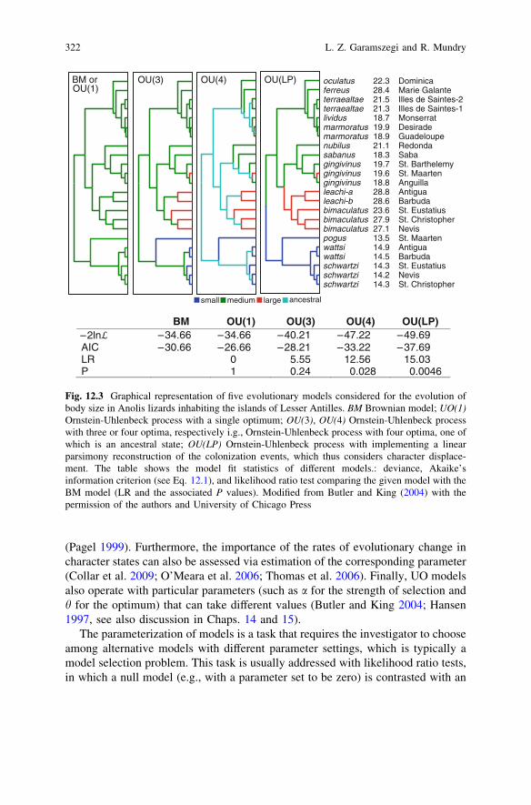
To demonstrate the use of model selection to choose among different evolu-tionary models, we provide an example from Butler and King (2004), but otherillustrative analyses are also available in the literature (Collar et al. 2009, 2011;Harmon et al. 2010; Hunt 2006; Lajeunesse 2009; Scales et al. 2009). Butler andKing (2004) re-examined character displacement in Anolis lizards on the LesserAntilles, where lizards live either in sympatry or in allopatry. Where two speciescoexist, these differ substantially in size, while on islands that are inhabited byonly one species, lizards are of intermediate size. Therefore, one can hypothesizethat body size differences on sympatric islands result from character displacement(i.e., when two intermediate-sized species came into contact with one anotherwhen colonizing an island, they subsequently diverged into a different direction).This hypothesis can be evaluated using alternative models of body size evolutionthat differ in the degree of how they incorporate processes due to directionalselection and character displacement. The authors, therefore, evaluated five dif-ferent models: (1) BM; (2) an OU process with a single optimum; (3) an OUprocess with three optima corresponding to large, intermediate, and small bodysize; (4) another OU model that includes an additional parameter to the three-optima model to deal with the adaptive regimes occurring on the internal branchesas an estimable ancestral state; and (5) a model implementing a linear parsimonyreconstruction of the colonization events (arrival history of species on the islands).Only the last model assumes character displacement. These models were com-pared by different methods including AIC, a Bayesian (Schwarz’s) informationcriterion (SIC), and likelihood ratio tests that unanimously revealed that the best-fitting model was the OU model with the reconstructed colonization events(Fig. 12.3). Altogether, the results support the hypothesis that character dis-placement had an effect on the evolution of body size in Anolis lizards that col-onized the Lesser Antilles.

12.3.4.2 Parameterization of Models

Another way to cope with the mode of evolution and to improve the fit of anymodel can be achieved by the appropriate setting of parameters that describe thefine details of the evolutionary process. For example, BM models can be adjustedusing the parameters j, d, or k that apply different branch-length transformationson the phylogeny (e.g., j stretches or compresses phylogenetic branch lengths andthus can be used to model trait evolution along a gradient from punctuational togradual evolution, while d scales overall path lengths in the phylogeny and thuscan be used to characterize the tempo of evolution) or that assess the contributionof the phylogeny (k weakens or strengthens the phylogenetic signal in the data)

12 Multimodel-Inference in Comparative Analyses 321

(Pagel 1999). Furthermore, the importance of the rates of evolutionary change incharacter states can also be assessed via estimation of the corresponding parameter(Collar et al. 2009; O’Meara et al. 2006; Thomas et al. 2006). Finally, UO modelsalso operate with particular parameters (such as a for the strength of selection andh for the optimum) that can take different values (Butler and King 2004; Hansen1997, see also discussion in Chaps. 14 and 15).

The parameterization of models is a task that requires the investigator to chooseamong alternative models with different parameter settings, which is typically amodel selection problem. This task is usually addressed with likelihood ratio tests,in which a null model (e.g., with a parameter set to be zero) is contrasted with an

BM or OU(3) OU(4)

pogus

schwartzi

schwartzischwartzi

wattsiwattsi

bimaculatus

bimaculatusbimaculatus

leachi-bleachi-a

nubilussabanusgingivinus

gingivinusgingivinus

oculatusferreus

lividus

marmoratusmarmoratus

terraealtaeterraealtae

OU(LP)

small medium large ancestral

OU(1)DominicaMarie GalanteIlles de Saintes-2Illes de Saintes-1MonserratDesiradeGuadeloupeRedondaSabaSt. BarthelemySt. MaartenAnguillaAntiguaBarbudaSt. EustatiusSt. ChristopherNevisSt. MaartenAntiguaBarbudaSt. EustatiusNevisSt. Christopher

22.328.421.521.318.719.918.921.118.319.719.618.828.828.623.627.927.113.514.914.514.314.214.3

BM OU(1) OU(3) OU(4) OU(LP)–2ln –34.66 –34.66 –40.21 –47.22 –49.69AIC –30.66 –26.66 –28.21 –33.22 –37.69LR 0 5.55 12.56 15.03P 1 0.24 0.028 0.0046

Fig. 12.3 Graphical representation of five evolutionary models considered for the evolution ofbody size in Anolis lizards inhabiting the islands of Lesser Antilles. BM Brownian model; UO(1)Ornstein-Uhlenbeck process with a single optimum; OU(3), OU(4) Ornstein-Uhlenbeck processwith three or four optima, respectively i.g., Ornstein-Uhlenbeck process with four optima, one ofwhich is an ancestral state; OU(LP) Ornstein-Uhlenbeck process with implementing a linearparsimony reconstruction of the colonization events, which thus considers character displace-ment. The table shows the model fit statistics of different models.: deviance, Akaike’sinformation criterion (see Eq. 12.1), and likelihood ratio test comparing the given model with theBM model (LR and the associated P values). Modified from Butler and King (2004) with thepermission of the authors and University of Chicago Press

322 L. Z. Garamszegi and R. Mundry

alternative model (e.g., with a parameter set to a nonzero value). If the test turnsout significant, the alternative model is accepted and used for further analyses(e.g., tests for correlations between traits) and for making evolutionary implica-tions. Another strategy is to evaluate the ML surface of the parameter space andthen set the parameter to the value where it reveals the maximum likelihood (i.e.,the strategy that most PGLS methods apply). Furthermore, AIC-based informa-tion-theoretic approaches can be used to obtain the parameter combinations thatoffer the best fit to the data.4

However, such a best model approach is not always straightforward. Parameterstates can span a continuous scale, and it is possible that a broad range ofparameter values are similarly likely. For example, the optimal phylogeneticscaling parameter k is usually estimated using maximum likelihood. This esti-mation might be robust if the peak of the likelihood surface is well defined (i.e.,few parameter states in a narrow range have a very high likelihood, while theremaining spectrum falls into a small likelihood region, Fig. 12.4, upper panels).Our experience, however, is that the likelihood surfaces are rather flat and varyconsiderably if single species are added or removed from the analysis (especiallyat modest interspecific sample sizes, Freckleton et al. 2002). This means that abroad range of parameter values describe the data similarly well (Fig. 12.4, lowerpanels), thus arbitrarily choosing a single parameter value on a flattish surface forfurther analysis may be deceiving.

We suggest that such uncertainty in parameter estimation can easily be incor-porated using model averaging. Applying the philosophy that we followed fordealing with multiple trees or scenarios for the correction for heterogeneous dataquality, we can also estimate the parameters of interest (e.g., ancestral state, slope,or correlation between two traits) at a wide range of the settings of the evolu-tionary parameters. Given that IT-based approaches typically compare sets ofdiscrete models, we need to create a large number of categories for the continuousparameter (e.g., by defining a finite number, such as 100 or 1,000, bins for k inincreasing order between the interval of 0–1) that can be used to condition dif-ferent models. Then, inference across this large number of models based on theirrelative fit to the data can be made, and given that intermediate states between thelarge number of categories are meaningful, interpretations can be extended to acontinuous scale. Therefore, evolutionary conclusions can be formulated based onthe parameter estimates that are averaged across models receiving different levelsof support instead of obtaining them from a single model. In theory, k can bemodel averaged as well, but when the maximum likelihood surface is flat (meaningthat many models with different ks will have similar AIC), deriving a single meanestimate may be misleading. In such a situation, only estimates together with theirmodel-averaged standard errors (or confidence intervals) make sense.

In the OPM, we show for k how this model averaging works in practice. Wealso provide examples for the case when the exercise for model parameters is

4 As long as the number of parameters is equal, AIC and ML reveal the same.

12 Multimodel-Inference in Comparative Analyses 323

combined with multimodel inference for statistical weights (Fig. 12.5). We keepon emphasizing that our suggestions merely stand on theoretical grounds; theperformance of model averaging in dealing with the uncertainty of modelparameterizations awaits future tests (based on both empirical and simulated data).

0.0 0.2 0.4 0.6 0.8 1.0 0.0 0.2 0.4 0.6 0.8 1.0

0.0 0.2 0.4 0.6 0.8 1.0 0.0 0.2 0.4 0.6 0.8 1.0

lambda

log-likelihood

Fig. 12.4 Typical shapes of maximum likelihood surfaces of the phylogenetic scaling factorlambda (k). The upper figures show two examples, in which the surface has a distinct peak andonly a narrow range of parameter values are likely. In contrast, the bottom graphs depict twocases in which the likelihood surface is rather flat, thus incurring a considerable uncertainty whenchoosing a single value. Vertical red lines give the values at the maximum likelihood. For theillustrative purposes, it is assumed that y-axes have the same scale

324 L. Z. Garamszegi and R. Mundry

12.3.5 The Performance of Different PhylogeneticComparative Methods

The logic of model selection can also be applied to assess whether any particularcomparative method is more appropriate than others. For example, in a meta-analysis, Jhwueng (2013) estimated the goodness of fit of four phylogeneticcomparative approaches. He collected more than a hundred comparative datasetsfrom the published literature, to which he applied the following methods to esti-mate the phylogenetic correlation between two traits: the non-phylogenetic model(i.e., treating the raw species data as being independent), the independent contrastsmethod (Felsenstein 1985), the autocorrelation method (Cheverud et al. 1985), thePGLS method incorporating the Ornstein-Uhlenbeck process (Martins and Hansen1997), and the phylogenetic mixed model (Hadfield and Nakagawa 2010; Lynch1991). Model fits obtained for different approaches were compared based on AIC,which revealed that the non-phylogenetic model and the independent contrastsmodel offered the best fit. However, the parameter estimates for the phylogeneticcorrelation were quite similar across models, indicating that the studied compar-ative methods were generally robust to describe evolutionary patterns present ininterspecific data.

omega

0.00.2

0.40.6

0.81.0 lambda0.0

0.20.4

0.6 0.8 1.0

log-

likel

ihoo

d

-80

-70

-60

-50

-40

-30

Fig. 12.5 Likelihood surface when the phylogenetic signal (lambda, k) and the data heteroge-neity (omega, x) parameters are estimated in a set of models using different parametercombinations for the brain size/body size evolution in primates (data are shown in Fig. 12.1). Thesurface shows the log-likelihoods of a large number of fitted models that differ in their k and xparameters. These parameters are allowed to vary between 0 and 1 (with steps of 0.01) in allpossible combinations. For a definition of x, see Fig. 12.2

12 Multimodel-Inference in Comparative Analyses 325

12.4 Further Applications

So far, we mostly focused on the potential that the IT framework provides inassociation with the PGLS framework, when models are fitted with ML. However,multimodel inference also makes sense in a broader context, and related issues areknown to exist in a range of other phylogenetic situations. We provide someexamples below (without the intention of being exhaustive), but further applica-tions can also be envisaged. This short list may illustrate that the benefits ofmultimodel inference can be efficiently exploited in relation to interspecific data.

A typical model selection problem is present in phylogenetics, when the interestis to find the best model that describes patterns of evolution for a given nucleotideor amino acid sequence. As briefly discussed in Chap. 2 (but see in-depth dis-cussion in Alfaro and Huelsenbeck 2006; Arima and Tardella 2012; Posada andBuckley 2004; Ripplinger and Sullivan 2008), several models have been devel-oped to deal with different substitution rates and base frequencies that ultimatelyinfluence the evolutionary outcome. The reliance on different models for phylo-genetic reconstructions can result in phylogenetic trees that vary in their branchingpattern and the underlying stochastic processes of nucleotide sequence changesthat generate branch lengths. Given that a priori information about the appropri-ateness of different evolutionary models is generally lacking, those who wish toestablish a phylogenetic hypothesis from molecular sequences are often confrontedwith a model selection problem. Accordingly, several evolutionary models need tobe fitted to the sequence data, and the one that offers the best fit (e.g., as revealedby likelihood ratio test or an AIC-based comparison or Bayesian methods) shouldbe used for further inferences about the phylogenetic relationships.

An intriguing example for the application of IT approaches in the phylogeneticcontext is the use of likelihood methods to detect temporal shifts in diversificationrates. By fitting a set of rate-constant and rate-variable birth–death models tosimulated phylogenetic data, Rabosky (2006) investigated which rate parametercombination (e.g., rate constant or rate varying over time) results in the model withthe lowest AIC. The results suggested that selecting the best model in this waycauses inflated Type I error, but when correcting for such error rates, the birth–death likelihood approach performed convincingly.

Eklöf et al. (2012) applied IT methods to understand the role of evolutionaryhistory for shaping ecological interaction networks. The authors approached theeffect of phylogeny by partitioning species into taxonomic units (e.g., fromkingdom to genus) and then by investigating which partitioning best explained thespecies’ interactions. This comparison was based on likelihood functions thatdescribed the probability that the considered partition structure reproduces the realdata obtained for nine published food webs. Furthermore, they also used marginallikelihoods (i.e., Bayes factors) to accomplish model selection across taxonomicranks. The major finding of the study was that models considering taxonomic

326 L. Z. Garamszegi and R. Mundry

partitions (i.e., phylogenetic relationships) offered better fit to the data, and foodwebs are best explained by higher taxonomic units (kingdom to class). Theseresults show that evolutionary history is important for understanding how com-munity structures are assembled in nature.

Depraz et al. (2008) evaluated competing hypotheses about the postglacialrecolonization history of the hairy land snail Trochulus villosus by using AIC-based model selection. They compared four refugia hypotheses (two refugia, threerefugia, alpine refugia, and east–west refugia models) that could account for thephylogeographic history of 52 populations. The four hypotheses were translatedinto migration matrices, with maximum likelihood estimates of migration rates.These models were challenged with the data, and Akaike weights were used tomake judgments about relative model support. This exercise revealed that themodel considering the two refugia hypothesis overwhelmingly offered the best fit.

In a phylogenetic comparative study based on ancestral state reconstruction,Goldberg and Igic (2008) investigated ‘Dollo’s law’ which states that complextraits cannot re-evolve in the same manner after loss. When using simulated dataand an NHST approach (likelihood ratio tests), they found that in most of the casesthe true hypothesis about the irreversibility of characters was falsely rejected.However, when using appropriate model selection (based on AIC-based ITmethods), the false rejection rate of ‘Dollo’s law’ was reduced.

Alfaro et al. (2009) developed an algorithm they called MEDUSA, which is anAIC-based stepwise approach that can detect multiple shifts in birth and death rateson an incompletely resolved phylogeny. This comparative method estimates rates ofspeciation and extinction by integrating information about the timing of splits alongthe backbone of a phylogenetic tree with known taxonomic richness. Diversificationanalyses are carried out by first finding the maximum likelihood for the per-lineagerates of speciation and extinction at a particular combination of phylogeny andspecies richness and then comparing these models across different combinations.

Further examples, e.g., for detecting convergent evolution based on stepwiseAIC (Ingram and Mahler 2013) and for revealing phylogenetic paths based on theC-statistic Information Criterion (von Hardenberg and Gonzalez-Voyer 2013) canbe found in Chaps. 18 and 8, respectively.

12.5 Concluding Remarks

What we have proposed here are several approaches to exploit the strengths of IT-based inference in the context of phylogenetic comparative methods. Using ITmethods such as model selection in combination with phylogenetic comparativemethods seems to offer the potential to elegantly solve problems which otherwisewould be hard to tackle. Other IT methods such as model averaging allow dealingwith phylogenetic uncertainty by explicitly incorporating it into the analysis and

12 Multimodel-Inference in Comparative Analyses 327

exploring to what extend it compromises certainty about the results. Takentogether, IT-based methods offer a great potential since they relieve researchersfrom the need of making arbitrary and/or poorly grounded decisions in favor ofone or the other model. Instead, they allow dealing easily with such uncertaintiesor, at least, allow an assessment of their magnitude (among the set of potentialmodels). Uncertainty is at the heart of our understanding about nature; thus, sta-tistical methods are needed that appreciate this attribute instead of neglecting it.

We need to stress, though, that our propositions are based on theoreticalgrounds and need to be tested before they can be trusted. Particularly, simulationstudies (e.g., along the design in Box 12.1) seem suitable for this purpose sincethey allow to investigate to what extend our propositions are able to reconstruct‘truth’ which otherwise (i.e., in the case of using empirical data) is simplyunknown. Simulation studies are warranted because the use of AIC (and other ITmetrics) to non-nested models (which was largely the case here) is somewhatcontroversial (Schmidt and Makalic 2011). Another cautionary remark is that werefrained ourselves to suggest that only the IT-based model selection can be usedto address the problems we raised. We envisage this discussion to serve as aninitiative for comparative studies to consider the suggested methods as additions tothe already existing toolbox, which yet await further exploitation.

Since the philosophy of IT-based inference is rather different from that of theclassical NHST approach and since the two approaches are quite frequently mixedin an inappropriate way (e.g., selecting the best model using AIC and then testingit using NHST), we feel that some warnings on the use of the IT approach might beuseful (particularly for those who were trained in NHST): IT-based inference doesnot reveal something like a ‘significance,’ and the two approaches must not becombined (Burnham and Anderson 2002; Mundry 2011). In the context of ourpropositions, this means that at least part of them naturally preclude the use ofsignificance tests. This is particularly the case when sets of models with differentcombinations of predictors and/or sets of different phylogenetic trees are investi-gated. The end result of such an exercise is a number of AIC values associatedwith a set of models. Selecting the best model using AIC and then testing itssignificance is inappropriate. Rather, one could model average the estimates andtheir standard errors (but not the P values!) or also the fitted values and explore towhat extend these vary across the different trees. Furthermore, one could useAkaike weights to infer about the relative importance of the different predictors.However, some of our proposed approaches might not necessarily and completelyrule out the use of classical NHST. In fact, we do not argue against using NHST,which we regard as a scientifically sound approach if used and interpreted cor-rectly. What we recommend is to not combine the use of significance tests withany of the approaches we suggested and draw inference solely on the basis of ITmethods (e.g., Akaike weights or evidence ratios).

328 L. Z. Garamszegi and R. Mundry

References

Alfaro ME, Huelsenbeck JP (2006) Comparative performance of Bayesian and AIC-basedmeasures of phylogenetic model uncertainty. Syst Biol 55(1):89–96. doi:10.1080/10635150500433565

Alfaro ME, Santini F, Brock C, Alamillo H, Dornburg A, Rabosky DL, Carnevale G, Harmon LJ(2009) Nine exceptional radiations plus high turnover explain species diversity in jawedvertebrates. Proc Natl Acad Sci. doi:10.1073/pnas.0811087106

Arima S, Tardella L (2012) Improved harmonic mean estimator for phylogenetic model evidence.J Comput Biol 19(4):418–438. doi:10.1089/cmb.2010.0139

Arnold C, Matthews LJ, Nunn CL (2010) The 10kTrees website: a new online resource forprimate hylogeny. Evol Anthropol 19:114–118

Bennett PM, Harvey PH (1985) Brain size, development and metabolism in birds and mammals.J Zool 207:491–509

Blomberg S, Garland TJ, Ives AR (2003) Testing for phylogenetic signal in comparative data:behavioral traits are more laible. Evolution 57:717–745

Bolker B (2007) Ecological models and data in R. Princeton University Press, Princeton andOxford

Burnham KP, Anderson DR (2002) Model selection and multimodel inference: a practicalinformation-theoretic approach. Springer, New York

Burnham KP, Anderson DR, Huyvaert KP (2011) AIC model selection and multimodel inferencein behavioral ecology: some background, observations, and comparisons. Behav EcolSociobiol 65(1):23–35

Butler MA, King AA (2004) Phylogenetic comparative analysis: a modeling approach foradaptive evolution. Am Nat 164(6):683–695. doi:10.1086/426002

Chamberlin TC (1890) The method of multiple working hypotheses. Science 15:92–96Cheverud JM, Dow MM, Leutenegger W (1985) The quantitative assessment of phylogenetic

constraints in comparative analyses: sexual dimorphism of body weight among primates.Evolution 39:1335–1351

Claeskens C, Hjort NL (2008) Model selection and model averaging. Cambridge UniversityPress, Cambridge

Cohen J (1994) The earth is round (p \ .05). Am Psychol 49(12):997–1003Collar DC, O’Meara BC, Wainwright PC, Near TJ (2009) Piscivory limits diversification of

feeding morphology in centrarchid fishes. Evolution 63:1557–1573Collar DC, Schulte JA, Losos JB (2011) Evolution of extreme body size disparity in monitor

lizards (Varanus). Evolution 65(9):2664–2680. doi:10.1111/j.1558-5646.2011.01335.xCongdon P (2003) Applied bayesian modelling. Wiley, ChichesterCongdon P (2006) Bayesian statistical modelling, 2nd edn. Wiley, Chichesterde Villemereuil P, Wells JA, Edwards RD, Blomberg SP (2012) Bayesian models for

comparative analysis integrating phylogenetic uncertainty. BMC Evol Biol 12. doi:10.1186/1471-2148-12-102

Depraz A, Cordellier M, Hausser J, Pfenninger M (2008) Postglacial recolonization at a snail’space (Trochulus villosus): confronting competing refugia hypotheses using model selection.Mol Ecol 17(10):2449–2462. doi:10.1111/j.1365-294X.2008.03760.x

Eklof A, Helmus MR, Moore M, Allesina S (2012) Relevance of evolutionary history for foodweb structure. Proc Roy Soc B-Biol Sci 279(1733):1588–1596. doi:10.1098/rspb.2011.2149

Felsenstein J (1985) Phylogenies and the comparative method. Am Nat 125:1–15Freckleton RP, Harvey PH, Pagel M (2002) Phylogenetic analysis and comparative data: a test

and review of evidence. Am Nat 160:712–726Gamerman D, Lopes HF (2006) Markov chain Monte Carlo: stochastic simulation for Bayesian

inference. CRC Press, Boca Raton, FLGaramszegi LZ (2011) Information-theoretic approaches to statistical analysis in behavioural

ecology: an introduction. Behav Ecol Sociobiol 65:1–11. doi:10.1007/s00265-010-1028-7

12 Multimodel-Inference in Comparative Analyses 329

Garamszegi LZ, Møller AP (2007) Prevalence of avian influenza and host ecology. Proc R Soc B274:2003–2012

Garamszegi LZ, Møller AP (2012) Untested assumptions about within-species sample size andmissing data in interspecific studies. Behav Ecol Sociobiol 66:1363–1373

Garamszegi LZ, Møller AP, Erritzøe J (2002) Coevolving avian eye size and brain size in relationto prey capture and nocturnality. Proc R Soc B 269:961–967

Goldberg EE, Igic B (2008) On phylogenetic tests of irreversible evolution. Evolution62(11):2727–2741. doi:10.1111/j.1558-5646.2008.00505.x

Hadfield JD, Nakagawa S (2010) General quantitative genetic methods for comparative biology:phylogenies, taxonomies and multi-trait models for continuous and categorical characters.J Evol Biol 23:494–508

Hansen TF (1997) Stabilizing selection and the comparative analysis of adaptation. Evolution51:1341–1351

Hansen TF, Bartoszek K (2012) Interpreting the evolutionary regression: the interplay betweenobservational and biological errors in phylogenetic comparative studies. Syst Biol 61:413–425

Harmon LJ, Losos JB, Jonathan Davies T, Gillespie RG, Gittleman JL, Bryan Jennings W, KozakKH, McPeek MA, Moreno-Roark F, Near TJ, Purvis A, Ricklefs RE, Schluter D, Schulte IiJA, Seehausen O, Sidlauskas BL, Torres-Carvajal O, Weir JT, Mooers AØ (2010) Early burstsof body size and shape evolution are rare in comparative data. Evolution 64(8):2385–2396.doi:10.1111/j.1558-5646.2010.01025.x

Hegyi G, Garamszegi LZ (2011) Using information theory as a substitute for stepwise regressionin ecology and behavior. Behav Ecol Sociobiol 65:69–76. doi:10.1007/s00265-010-1036-7

Hunt G (2006) Fitting and comparing models of phyletic evolution: random walks and beyond.Paleobiology 32(4):578–601. doi:10.1666/05070.1

Hutcheon JM, Kirsch JW, Garland TJ (2002) A comparative analysis of brain size in relation toforaging ecology and phylogeny in the chiroptera. Brain Behav Evol 60:165–180

Ingram T, Mahler DL (2013) SURFACE: detecting convergent evolution from comparative databy fitting Ornstein-Uhlenbeck models with stepwise Akaike information criterion. MethodsEcol Evol 4(5):416–425. doi:10.1111/2041-210x.12034

Ives AR, Midford PE, Garland T (2007) Within-species variation and measurement error inphylogenetic comparative methods. Syst Biol 56(2):252–270

Iwaniuk AN, Dean KM, Nelson JE (2004) Interspecific allometry of the brain and brain regions inparrots (Psittaciformes): comparisons with other birds and primates. Brain Behav Evol30:40–59

Jhwueng D-C (2013) Assessing the goodness of fit of phylogenetic comparative methods: a meta-analysis and simulation study. PLoS ONE 8(6):e67001. doi:10.1371/journal.pone.0067001

Johnson JB, Omland KS (2004) Model selection in ecology and evolution. Trends Ecol Evol19(2):101–108

Konishi S, Kitagawa G (2008) Information criteria and statistical modeling. Springer, New YorkKutsukake N, Innan H (2013) Simulation-based likelihood approach for evolutionary models of

phenotypic traits on phylogeny. Evolution 67(2):355–367Lajeunesse MJ (2009) Meta-analysis and the comparative phylogenetic method. Am Nat

174(3):369–381. doi:10.1086/603628Legendre P, Lapointe FJ, Casgrain P (1994) Modeling brain evolution from behavior: a

permutational regression approach. Evolution 48(5):1487–1499. doi:10.2307/2410243Link WA, Barker RJ (2006) Model weights and the foundations of multimodel inference.

Ecology 87:2626–2635Lynch M (1991) Methods for the analysis of comparative data in evolutionary biology. Evolution

45(5):1065–1080Martins EP (1996) Conducting phylogenetic comparative analyses when phylogeny is not known.

Evolution 50:12–22Martins EP, Hansen TF (1997) Phylogenies and the comparative method: a general approach to

incorporating phylogenetic information into the analysis of interspecific data. Am Nat149:646–667

330 L. Z. Garamszegi and R. Mundry

Massart P (ed) (2007) Concentration inequalities and model selection: ecole d’eté de probabilitésde Saint-Flour XXXIII - 2003. Springer, Berlin

Mundry R (2011) Issues in information theory-based statistical inference–a commentary from afrequentist’s perspective. Behav Ecol Sociobiol 65(1):57–68

Mundry R, Nunn CL (2008) Stepwise model fitting and statistical inference: turning noise intosignal pollution. Am Nat 173:119–123

Nakagawa S, Hauber ME (2011) Great challenges with few subjects: Statistical strategies forneuroscientists. Neurosci Biobehav Rev 35(3):462–473

O’Meara BC, Ané C, Sanderson MJ, Wainwright PC (2006) Testing for different rates ofcontinuous trait evolution using likelihood. Evolution 60(5):922–933. doi:10.1111/j.0014-3820.2006.tb01171.x

Pagel M (1999) Inferring the historical patterns of biological evolution. Nature 401:877–884Pagel M, Meade A, Barker D (2004) Bayesian estimation of ancestral character states on

phylogenies. Syst Biol 53(5):673–684Pagel M, Meade A (2006) Bayesian analysis of correlated evolution of discrete characters by

reversible-jump Markov chain Monte Carlo. Am Nat 167(6):808–825Posada D, Buckley TR (2004) Model selection and model averaging in phylogenetics: advantages

of Akaike information criterion and Bayesian approaches over likelihood ratio tests. Syst Biol53(5):793–808. doi:10.1080/10635150490522304

R Development Core Team (2013) R: a language and environment for statistical computing.R Foundation for Statistical Computing, Vienna, Austria. http://www.R-project.orgS

Rabosky DL (2006) Likelihood methods for detecting temporal shifts in diversification rates.Evolution 60(6):1152–1164

Ripplinger J, Sullivan J (2008) Does choice in model selection affect maximum likelihoodanalysis? Syst Biol 57(1):76–85. doi:10.1080/10635150801898920

Scales JA, King AA, Butler MA (2009) Running for your life or running for your dinner: whatdrives fiber-type evolution in lizard locomotor muscles? Am Nat 173:543–553

Schmidt D, Makalic E (2011) The behaviour of the Akaike information criterion when applied tonon-nested sequences of models. In: Li J (ed) AI 2010: advances in artificial intelligence, vol6464. Lecture Notes in Computer Science. Springer, Heidelberg, pp 223–232. doi:10.1007/978-3-642-17432-2_23

Stephens PA, Buskirk SW, Hayward GD, Del Rio CM (2005) Information theory and hypothesistesting: a call for pluralism. J Appl Ecol 42(1):4–12

Symonds MRE, Moussalli A (2011) A brief guide to model selection, multimodel inference andmodel averaging in behavioural ecology using Akaike’s information criterion. Behav EcolSociobiol 65(1):13–21

Terribile LC, Olalla-Tarraga MA, Diniz JAF, Rodriguez MA (2009) Ecological and evolutionarycomponents of body size: geographic variation of venomous snakes at the global scale. Biol JLinn Soc 98(1):94–109

Thomas GH, Freckleton RP, Székely T (2006) Comparative analyses of the influence ofdevelopmental mode on phenotypic diversification rates in shorebirds. Proc Roy Soc B-BiolSci 273(1594):1619–1624

von Hardenberg A, Gonzalez-Voyer A (2013) Disentangling evolutionary cause-effect relation-ships with phylogenetic confirmatory path analysis. Evolution 67(2):378–387. doi:10.1111/j.1558-5646.2012.01790.x

Whitmee S, Orme CDL (2013) Predicting dispersal distance in mammals: a trait-based approach.J Anim Ecol 82(1):211–221. doi:10.1111/j.1365-2656.2012.02030.x

Whittingham MJ, Stephens PA, Bradbury RB, Freckleton RP (2006) Why do we still usestepwise modelling in ecology and behaviour? J Anim Ecol 75:1182–1189

12 Multimodel-Inference in Comparative Analyses 331