chapter 12 bargaining and power in networks

Chapter 12

Bargaining and Power in Networks

From the book Networks, Crowds, and Markets: Reasoning about a Highly Connected World.By David Easley and Jon Kleinberg. Cambridge University Press, 2010.Complete preprint on-line at http://www.cs.cornell.edu/home/kleinber/networks-book/

In our analysis of economic transactions on networks, particularly the model in Chapter

11, we considered how a node’s position in a network affects its power in the market. In

some cases, we were able to come up with precise predictions about prices and power, but

in others the analysis left open a range of possibilities. For example, in the case of perfect

competition between traders, we could conclude that the traders would make no profit, but

it was not possible to say whether the resulting situation would favor particular buyers or

sellers — different divisions of the available surplus were possible. This is an instance of

a broader phenomenon that we discussed earlier, in Chapter 6: when there are multiple

equilibria, some of which favor one player and some of which favor another, we may need to

look for additional sources of information to predict how things will turn out.

In this chapter, we formulate a perspective on power in networks that can help us further

refine our predictions for the outcomes of different participants. This perspective arises

dominantly from research in sociology, and it addresses not just economic transactions, but

also a range of social interactions more generally that are mediated by networks. We will

develop a set of formal principles that aim to capture some subtle distinctions in how a

node’s network position affects its power. The goal will be to create a succinct mathematical

framework enabling predictions of which nodes have power, and how much power they have,

for arbitrary networks.

12.1 Power in Social Networks

The notion of power is a central issue in sociology, and it has been studied in many forms. Like

many related notions, a fundamental question is the extent to which power is a property of

individuals (i.e. someone is particularly powerful because of their own exceptional attributes)

Draft version: June 10, 2010

339

340 CHAPTER 12. BARGAINING AND POWER IN NETWORKS

and the extent to which it is a property of network structure (i.e. someone is particularly

powerful because they hold a pivotal position in the underlying social structure).

The goal here is to understand power not just as a property of agents in economic settings,

or in legal or political settings, but in social interaction more generally — in the roles people

play in groups of friends, in communities, or in organizations. A particular focus is on the

way in which power is manifested between pairs of people linked by edges in a larger social

network. Indeed, as Richard Emerson has observed in his fundamental work on this subject,

power is not so much a property of an individual as it is a property of a relation between

two individuals — it makes more sense to study the conditions under which one person has

power over another, rather than simply asserting that a particular person is “powerful” [148].

A common theme in this line of work is to view a social relation between two individuals

as producing value for both of them. We will be deliberately vague in specifying what this

value is, since it clearly depends on the type of social relation we are discussing, but the

idea adapts naturally to many contexts. In an economic setting, it could be the revenue that

two people can produce by working together; in a political setting, it could be the ability of

each person in the relationship to do useful favors for the other; in the context of friendship,

it could be the social or psychological value that the two people derive from being friends

with one another. In any of these examples, the value may be divided equally or unequally

between the two parties. For example, one of the two parties in the relationship may get

more benefit from it than the other — they may get more than half the profits in a joint

business relationship, or in the context of a friendship they may be the center of attention,

or get their way more often in the case of disagreements. The way in which the value in the

relationship is divided between the two parties can be viewed as a kind of social exchange,

and power then corresponds to the imbalance in this division — with the powerful party in

the relationship getting the majority of the value.

Now, in some cases this imbalance in a relationship may be almost entirely the result of

the personalities of the two people involved. But in other cases, it may also be a function

of the larger social network in which the two people are embedded — one person may be

more powerful in a relationship because they occupy a more dominant position in the social

network, with greater access to social opportunities outside this single relationship. In this

latter case, the imbalance in the relationship may be rooted in considerations of network

structure, and transcend the individual characteristics of the two people involved. The

ways in which social imbalances and power can be partly rooted in the structure of the

social network has motivated the growth of a research area in sociology known as network

exchange theory [417].

An Example of a Powerful Network Position. It is useful to discuss this in the

context of a simple example. Consider the group of five friends depicted in Figure 12.1,

12.1. POWER IN SOCIAL NETWORKS 341

A B C

D

E

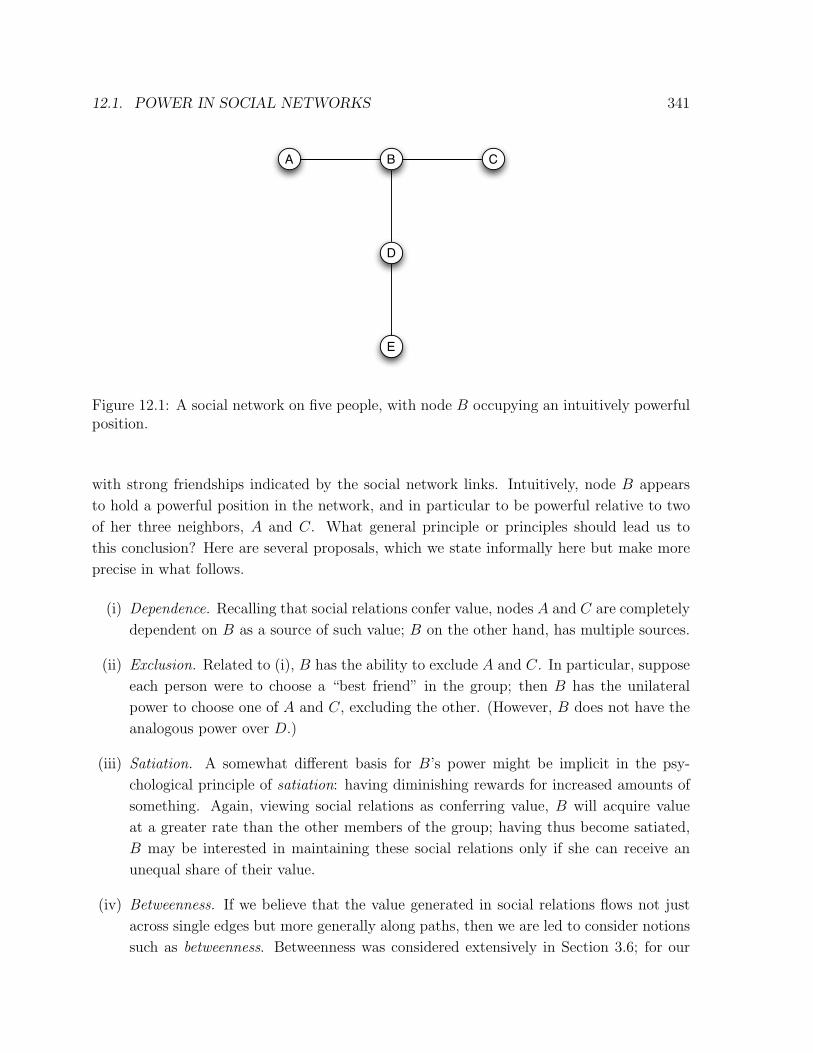
Figure 12.1: A social network on five people, with node B occupying an intuitively powerfulposition.

with strong friendships indicated by the social network links. Intuitively, node B appears

to hold a powerful position in the network, and in particular to be powerful relative to two

of her three neighbors, A and C. What general principle or principles should lead us to

this conclusion? Here are several proposals, which we state informally here but make more

precise in what follows.

(i) Dependence. Recalling that social relations confer value, nodes A and C are completely

dependent on B as a source of such value; B on the other hand, has multiple sources.

(ii) Exclusion. Related to (i), B has the ability to exclude A and C. In particular, suppose

each person were to choose a “best friend” in the group; then B has the unilateral

power to choose one of A and C, excluding the other. (However, B does not have the

analogous power over D.)

(iii) Satiation. A somewhat different basis for B’s power might be implicit in the psy-

chological principle of satiation: having diminishing rewards for increased amounts of

something. Again, viewing social relations as conferring value, B will acquire value

at a greater rate than the other members of the group; having thus become satiated,

B may be interested in maintaining these social relations only if she can receive an

unequal share of their value.

(iv) Betweenness. If we believe that the value generated in social relations flows not just

across single edges but more generally along paths, then we are led to consider notions

such as betweenness. Betweenness was considered extensively in Section 3.6; for our


purposes here, it is enough to think informally of a node as having high betweenness if

it lies on paths (and particularly short paths) between many pairs of other nodes. In

our example, B has high betweenness because she is the unique access point between

multiple different pairs of nodes in the network, and this potentially confers power.

More generally, betweenness is one example of a centrality measure that tries to find

the “central” points in a network. We saw in our discussion of structural holes in

Section 3.5 that evaluating a node’s power in terms of its role as an access point

between different parts of the network makes sense in contexts where we are concerned

about issues like the flow of information. Here, however, where we are concerned about

power arising from the asymmetries in pairwise relations, we will see some concrete

cases where a simple application of ideas about centrality can in fact be misleading.

12.2 Experimental Studies of Power and Exchange

While all of these principles are presumably at work in many situations, it is difficult to

make precise or quantify their effects in most real-world settings. As a result, researchers have

turned to laboratory experiments in which they ask test subjects to take part in stylized forms

of social exchange under controlled conditions. This style of research grew into an active

experimental program carried out by a number of research groups in network exchange theory

[417]. The basic idea underlying the experiments is to take the notion of “social value” and

represent it under laboratory conditions using a concrete economic framework, of the type

that we have seen in Chapters 10 and 11. In these experiments, the value that relationships

produce is represented by an amount of money that the participants in a relationship get

to share. This does not mean, however, that an individual necessarily cares only about the

amount of money that he receives. As we shall see, it’s clear from the results that even

subjects in the experiments may also care about other aspects of the relationship, such as

the fairness of the sharing.

While the details vary across experiments, here is the set-up for a typical one. Roughly,

people are placed at the nodes of a small graph representing a social network; a fixed sum

of money is placed on each edge of a graph; and nodes joined by an edge negotiate over how

the money placed between them should be divided up. The final, crucial part of the set-up

is that each node can take part in a division with only one neighbor, and so is faced with

the choice not just of how large a share to seek, but also with whom. The experiment is run

over multiple periods to allow for repeated interaction by the participants, and we study the

divisions of money after many rounds.

Here are the mechanics in more detail.

1. A small graph (such as the one in Figure 12.1) is chosen, and a distinct volunteer

test subject is chosen to represent each node. Each person, representing a node, sits

12.2. EXPERIMENTAL STUDIES OF POWER AND EXCHANGE 343

at a computer and can exchange instant messages with the people representing the

neighboring nodes.

2. The value in each social relation is made concrete by placing a resource pool on each

edge — let’s imagine this as a fixed sum of money, say $1, which can be divided between

the two endpoints of the edge. We will refer to a division of this money between the

endpoints as an exchange. Whether this division ends up equal or unequal will be

taken as a sign of the asymmetric amounts of power in the relationship that the edge

represents.

3. Each node is given a limit on the number of neighbors with whom she can perform

an exchange. The most common variant is to impose the extreme restriction that

each node can be involved in a successful exchange with only one of her neighbors;

this is called the 1-exchange rule. Thus, for example, in Figure 12.1, node B can

ultimately make money from an exchange with only one of her three neighbors. Given

this restriction, the set of exchanges that take place in a given round of the experiment

can be viewed as a matching in the graph: a set of edges that have no endpoints in

common. However, it will not necessarily be a perfect matching, since some nodes may

not take part in any exchange. For example, in the graph in Figure 12.1, the exchanges

will definitely not form a perfect matching, since there are an odd number of nodes.

4. Here is how the money on each edge is divided. A given node takes part in simultaneous

sessions of instant messaging separately with each of her neighbors in the network. In

each, she engages in relatively free-form negotiation, proposing splits of the money on

the edge, and potentially reaching an agreement on a proposed split. These negotiations

must be concluded by a fixed time limit; and to enforce the 1-exchange rule defined

above, as soon as a node reaches an agreement with one neighbor, her negotiations

with all other neighbors are immediately terminated.

5. Finally, the experiment is run for multiple rounds. The graph and the assignment

of subjects to nodes as described in point (1) are kept fixed across rounds. In each

round, new money is placed on each edge as in point (2), each node can take part in

an exchange as in point (3), and the money is divided as in point (4). The experiment

is run for multiple rounds to allow for repeated interactions among the nodes, and we

study the exchange values that occur after many rounds.

Thus the general notion of “social value” on edges is implemented using a specific eco-

nomic metaphor: the value is represented using money, and people are negotiating explicitly

over how to divide it up. We will mainly focus on the 1-exchange rule, unless noted other-

wise. We can view the 1-exchange rule as encoding the notion of choosing “best friends”,

which we discussed earlier when we talked about exclusion. That is, the 1-exchange rule


A B

(a) 2-Node Path

A B C

(b) 3-Node Path

A B C D

(c) 4-Node Path

A B C D E

(d) 5-Node Path

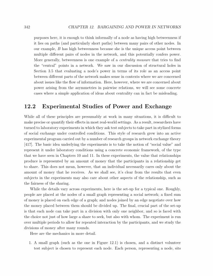
Figure 12.2: Paths of lengths 2, 3, 4, and 5 form instructive examples of different phenomenain exchange networks.

models a setting in which the nodes are trying to form partnerships: each node wants to be

in a partnership; and subject to this, the node wants to get a reasonable share of the value

implicit in this partnership. Later in this chapter we will see that varying the number of

successful exchanges in which a node can participate has effects on which nodes hold power,

often in interesting ways.

There are many variations in the precise way these experiments are implemented. One

particularly interesting dimension is the amount of information provided to the participants

about the exchanges made by other participants. This has ranged in experiments from a

high-information version — in which each person sees not just what is happening on their

edges, but also what is happening on every edge in the network, in real-time — to a low-

information version — in which each person is told only what is happening on the edges

she is directly involved in; for example, she may have no idea how many other potential

partners each of her neighbors has. An interesting finding from this body of work is that

the experimental results do not change much with the amount of information available [389];

this suggests a certain robustness to the results, and also allows us to draw some conclusions

about the kinds of reasoning that participants are engaging in as they take part in these

experiments.

12.3 Results of Network Exchange Experiments

Let’s start by discussing what happens when one runs this type of experiment on some

simple graphs using human test subjects. Since the results are intuitively reasonable and

fairly robust, we’ll then consider — in increasing levels of detail — what sorts of principles

can be inferred about power in these types of exchange situations.

Figure 12.2 depicts four basic networks that have been used in experiments. Notice

that these are just paths of lengths 2, 3, 4, and 5. Despite their simplicity, however, each

12.3. RESULTS OF NETWORK EXCHANGE EXPERIMENTS 345

introduces novel issues, and we will discuss them in order.

The 2-Node Path. The 2-node path is as simple as it gets: two people are given a

fixed amount of time in which to agree on a way to split $1. Yet even this simple setting

introduces a lot of conceptual complexity — a large amount of work in game theory has

been devoted precisely to the problem of reasoning about outcomes when two parties with

oppositely aligned interests sit down to negotiate. As we will discuss more fully later in this

chapter, most of the standard theoretical treatments predict a 12 -

12 split. This seems to be

a reasonable prediction, and it is indeed approximately what happens in network exchange

experiments on a 2-node graph.

The 3-Node Path. On a 3-node path with nodes labeled A, B, and C in order, node B

intuitively has power over both A and C. For example, as B negotiates with A, she has the

ability to fall back on her alternative with C, while A has no other alternatives. The same

reasoning applies to B’s negotiations with C.

Moreover, at least one of A or C must be excluded from an exchange in each round. In

experiments, one finds that subjects who are excluded tend to ask for less in the next round

in the hope of becoming included. Thus, the repeated exclusion of A and C tends to drive

down what they ask for, and one finds in practice that B indeed receives the overwhelming

majority of the money in her exchanges (roughly 5/6 in one recent set of experiments [281]).

An interesting variation on this experiment is to modify the 1-exchange rule to allow B

to take part in two exchanges in each round. One now finds that B negotiates on roughly

equal footing with both A and C. This is consistent with the notions of dependence and

exclusion discussed earlier: in order for B to achieve half the value from each exchange in

each round, she needs A and C as much as they need her.

This result for the version in which B is allowed two exchanges is less consistent with

satiation, however: if B were becoming satiated by money twice as quickly as A and C, one

could expect to start seeing an effect in which A and C need to offer unequal splits to B in

order to keep B interested. But this is not what actually happens.

The 4-Node Path. The 4-node path is already significantly more subtle than the previous

two examples. There is an outcome in which all nodes take part in an exchange — A

exchanges with B and C exchanges with D — but there is also an outcome in which B and

C exchange with each other while excluding A and D.

Thus, B should have some amount of power over A, but it is a weaker kind of power

than in the 3-node path. In the 3-node path, B could exclude A and seek an exchange with

C, who has no other options. In the 4-node path, on the other hand, if B excludes A, then

B herself pays a price by having to seek an exchange with C, who already has an attractive


A B

C

D

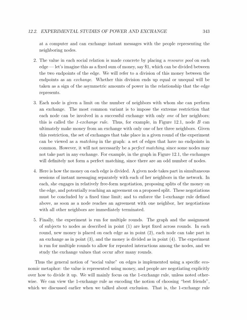
Figure 12.3: An exchange network with a weak power advantage for node B.

alternative in D. In other words, B’s threat to exclude A is a costly one to actually execute.

Experiments bear out this notion of weak power: in A-B exchanges, B gets roughly between

7/12 and 2/3 of the money, but not more [281, 373].

The 5-Node Path. Paths of length 5 introduce a further subtlety: node C, which intu-

itively occupies the “central” position in the network, is in fact weak when the 1-exchange

rule is used. This is because C’s only opportunities for exchange are with B and D, and

each of these nodes have very attractive alternatives in A and E respectively. Thus, C can

be excluded from exchange almost as easily as A and E can. Put succinctly, C’s partners

for negotiation all have access to very weak nodes as alternatives, and this makes C weak as

well.

In experiments, one finds that C does slightly better than A and E do, but only slightly.

Thus, the 5-node path shows that simple centrality notions like betweenness can be mislead-

ing measures of power in some kinds of exchange networks.

Note that the weakness of C really does depend on the fact that the 1-exchange rule

is used. Suppose, for example, that we instead allowed A, C, and E to take part in one

exchange each, but allowed B and D to take part in two exchanges each. Then suddenly

each of B and D need C to make full use of their exchange opportunities, and C is now the

node with the ability to exclude some of his exchange partners.

Other Networks. Many other networks have been studied experimentally. In a number

of cases, the outcomes can be understood by combining ideas from the four basic networks

in Figure 12.2.

For example, the graph in Figure 12.1 has been extensively studied by network exchange

theorists. Since B has the ability to exclude both A and C, she tends to achieve highly favor-

able exchanges with them. Given these two alternatives, B and D almost never exchange;

as a result, D doesn’t have a realistic second option besides E, and hence D and E tend to

12.3. RESULTS OF NETWORK EXCHANGE EXPERIMENTS 347

A

B C

Figure 12.4: An exchange network in which negotiations never stabilize.

exchange on roughly equal footing. All these observations are borne out by the experimental

results.

Another interesting example that has been extensively studied is the “stem graph” shown

in Figure 12.3. Here, C and D typically exchange with each other, while B exchanges with

A, obtaining favorable terms. The position of node B in this network is conceptually similar

to the position of B in the 4-node-path: in the stem graph, B has a power advantage in her

dealings with A, but it is a weak power advantage, since to exclude A she has to exchange

with C or D, who each have exchange options in each other. Experiments have shown that

node B in the stem graph makes slightly more money than node B in the 4-node path, and

there is an intuitive, if somewhat subtle, reason for this: B’s threat over A in the 4-node

path is to negotiate with the comparably powerful node C, while B’s threat in the stem

graph is to negotiate with people who are slightly weaker.

An Unstable Network. A common theme in all the networks we have discussed thus far

is that the negotiations among participants tend to wrap up reliably by the time limit, with

fairly consistent outcomes. But there exist pathological networks in which negotiations tend

to drag out until the very end, with unpredictable individual outcomes for the participants.

To see why this might happen, we consider the simplest of these pathological examples,

depicted in Figure 12.4: three nodes each connected to each other. It is not hard to see what

happens when an exchange experiment is run on the triangle. Only one exchange can be

completed among the three nodes; so as time is running out, two of the nodes — say, A and

B — will be wrapping up negotiations, while the third node (C in this case) is completely

left out and stands to get nothing. This means that C will be willing to break into the A-B

negotiations up to the very end, offering an exchange to either of these nodes in which they

get almost everything as long as C can get a small amount. If this happens — say that C

breaks up the A-B negotiations by offering highly favorable terms to A — then there will be

a different node left out (B in this case), who will in turn be willing to offer highly favorable

terms to get back in on an exchange.

This process, by itself, would cycle indefinitely — with some node always left out and


A

B

C

D

sells to A for x: payoff of x

receives good of value 1: payoff of 1-x

Figure 12.5: An exchange network built from the 4-node path can also be viewed as abuyer-seller network with 2 sellers and 2 buyers.

trying anything to get back in — and it is only brought to a halt by the arbitrary arrival of

the time limit. Under these conditions, you have nodes “playing for the last shot,” with the

outcome for any one node correspondingly hard to predict.

Again, this is not an issue that comes up in any of the earlier examples we discussed;

what’s different in the triangle network is that no matter what tentative exchanges are being

planned, excluded nodes have a natural way to “break in” to the negotiations. This prevents

the outcome from ever stabilizing across the network. It is also worth noting that the mere

presence of a triangle in a larger network does not necessarily cause problems: for example,

the stem graph in Figure 12.3 contains a triangle, but the exchange possibilities provided by

the additional node A allows for robust outcomes in which A exchanges with B and C and D

exchange with each other. The problem with a “free-standing” triangle as in Figure 12.4 is

fundamentally different: here, there is always a node who is left out, and yet has the ability

to do something about it.

12.4 A Connection to Buyer-Seller Networks

When we discussed matching markets in Chapter 10, we considered bipartite graphs con-

sisting of buyers and sellers. Here, on the other hand, we have been talking about graphs in

which the participants all play the same role (there is no division into buyers and sellers);

and rather than conducting trade, they negotiate over the division of money on the edges.

Despite these surface-level differences, there is a close connection between the two set-

tings. To see this connection, let’s consider the 4-node path as an example. Suppose we

12.5. MODELING TWO-PERSON INTERACTION: THE NASH BARGAINING SOLUTION349

declare nodes A and C to be buyers, and nodes B and D to be sellers. We give one unit of a

good to each of B and D, and one unit of money to each of A and C; we assume that A and

C each have a valuation of 1 for one copy of the good, and that B and D have no valuation

for the good. We now consider the prices at which sales of the good will take place.

It takes a bit of thought, but this is completely equivalent to the exchange network

experiment on the length-4 path, as indicated in Figure 12.5. For example, if B sells to A

for a price of x, then B gets a payoff of x (from the x units of money), and A gets a payoff

of 1− x (from the 1 unit of value for the good, minus the x units of money he has to pay).

Thus, the negotiation between A and B over a price x in the buyer-seller network is just like

the negotiation between A and B over the division of $1 into x and 1 − x in an exchange

network. Furthermore, the 1-exchange rule corresponds to the requirement that each seller

can only sell a single unit of the good, and each buyer only wants one unit of the good.

One can perform a comparable translation for all the graphs in Figures 12.1 and 12.2.

However, it is important to note two caveats about this general observation on the relation-

ship between exchange networks and buyer-seller networks. First, the translation is only

possible for graphs that are bipartite (as all the graphs in Figures 12.1 and 12.2 are), even if

they are not drawn with the nodes in two parallel columns. The triangle graph in Figure 12.4

is not bipartite, and although we can still talk about the exchange network experiment, it is

not possible to label the nodes as buyers and sellers in such a way that all edges join a seller

to a buyer. We can make one node a seller, and another node a buyer, but then we have

no options for what to label the third node. Similarly, the stem graph in Figure 12.3 is not

bipartite, and so the analogy to buyer-seller networks cannot be applied there either.

A second caveat is that, for bipartite graphs, the two formulations are equivalent only

at a mathematical level. It is not at all clear that human subjects placed in a buyer-seller

experiment would behave in the same way as human subjects in a network exchange exper-

iment, even on the very same graph. Indeed, there is recent empirical evidence suggesting

that one may in fact see different outcomes from these two ways of describing the same

process to test subjects [397].

12.5 Modeling Two-Person Interaction: The Nash Bar-gaining Solution

Thus far, we have seen a range of networks on which exchange experiments have been

carried out, and we have developed some of the informal reasons why the outcomes turn

out the way they do. We’d now like to develop a more mathematical framework allowing

us to express predictions about what will happen when network exchange takes place in an

arbitrary network. Among the phenomena we’d like to be able to explain are the distinctions

between equal and asymmetric division of value across an edge; between strong power (when


A B

outside option

x

outsideoption

y

Figure 12.6: Two nodes bargaining with outside options.

imbalances go to extremes) and weak power (as in the four-node path, when the imbalance

remains moderate); and between networks where outcomes stabilize and networks (like the

triangle in Figure 12.4) where they don’t.

In fact, we will be able to achieve this goal to a surprising extent, capturing each of

these phenomena in a model based on simple principles. We begin the formulation of this

model here and in the next section by developing two important ingredients, each based on a

different type of two-person interaction. The first ingredient — the Nash bargaining solution

— has a more mathematical flavor, while the second — the ultimatum game — is based

primarily on human-subject experiments.

The Nash Bargaining Solution. Let’s start with a simple formulation of two-person

bargaining. Suppose, as in network exchange on a 2-node path, that two people A and B

are negotiating over how to split $1 between them. Now, however, we extend the story to

assume that A also has an outside option of x, and B has an outside option of y. By this we

mean that if A doesn’t like his share of the $1 arising from the negotiations with B, he can

leave and take x instead. This will presumably happen, for instance, if A is going to get less

than x from the negotiations. Similarly, B has the option of abandoning the negotiation at

any time and taking her outside option of y. Notice that if x + y > 1, then no agreement

between A and B is possible, since they can’t divide a dollar so that one gets at least x and

the other gets at least y. Consequently, we will assume x+y ≤ 1 when we consider this type

of situation.

Given these conditions, A requires at least x from the negotiations over splitting the

dollar, and B requires at least y. Consequently, the negotiation is really over how to split

the surplus s = 1 − x − y (which is at least 0, given our assumption that x + y ≤ 1 in the

previous paragraph). A natural prediction is that if the two people A and B have equal

bargaining power, then they will agree on the division that splits this surplus evenly: A gets

x + 12s, and B gets y + 1

2s. This is the prediction of a number of general theories including

12.5. MODELING TWO-PERSON INTERACTION: THE NASH BARGAINING SOLUTION351

the Nash bargaining solution [312], and we will use this as our term for the outcome:

Nash Bargaining Solution: When A and B negotiate over splitting a dollar, with

an outside option of x for A and an outside option of y for B (and x + y ≤ 1),

the Nash bargaining outcome is

• x +1

2s =

x + 1− y

2to A, and

• y +1

2s =

y + 1− x

2to B.

In the literature on network exchange theory, this division is sometimes referred as the

equidependent outcome [120], since each person is depending equally on the other for conces-

sions to make the negotiation work. At a high level, the formulation of the Nash bargaining

solution emphasizes an important point about the process of negotiation in general: trying

to ensure that you have as strong an outside option as possible, before the negotiations even

begin, can be very important for achieving a favorable outcome. For most of this chapter,

it is enough to take the Nash bargaining solution as a self-contained principle, supported by

the results of experiments. In the final section of the chapter, however, we ask whether it

can be derived from more fundamental models of behavior. We show there that in fact it

can — it arises naturally as an equilibrium when we formulate the process of bargaining as

a game.

Experiments on Status Effects. When we think about bargaining in the context of

experiments with human subjects, we of course need to consider the assumption that the

two people have equal bargaining power. While in our models we will make use of this

assumption, it is interesting to think about how external information could affect relative

bargaining power in settings such as these.

The effects of perceived social status on bargaining power have been explored experimen-

tally by sociologists. In these experiments, two people are asked to divide money in situations

where they are led to believe that one is “higher-status” and the other is “lower-status.” For

example, in a recent set of these experiments, pairs of people A and B, each female college

sophomores, negotiated in the presence of outside options using instant messaging. How-

ever, each was given false information about the other: A was told that B was a high-school

student with low grades, while B was told that A was a graduate student with very high

grades [390]. Thus, A believed B to be low-status, while B believed A to be high-status.

The results of these experiments illustrate interesting ways in which beliefs about differ-

ential status can lead to deviations from theoretical predictions in bargaining. First, each

subject had to communicate information about their own outside options to their partners

as part of the negotiation (this information was not provided by the experimenters). It

was found that people tended to inflate the size of their outside option when they believed


their negotiating partner was lower-status; and they tended to reduce the size of their out-

side option when they believed their negotiating partner was higher-status. Compounding

this effect, people tended to partially discount a negotiating partner’s claims about outside

options when they believed this partner to be lower-status. (In other words, lower-status

people tended to underreport the value of their outside options, and even these underre-

ported values were discounted by their partners.) Overall, for these and other reasons, the

subject who was believed to be higher-status by her partner tended to achieve significantly

better bargaining outcomes than the theoretical predictions.

Naturally, these status effects are interesting additional factors to incorporate into models

of exchange. For developing the most basic family of models, however, we will focus on the

case of interaction in the absence of additional status effects, using the Nash bargaining

outcome as a building block.

12.6 Modeling Two-Person Interaction: The Ultima-tum Game

The Nash bargaining outcome provides us with a way of reasoning about two people whose

power differences arise through differences in their outside options. In principle, this applies

even to situations with extreme power imbalances. For example, in network exchange on a

3-node path, we saw that the center node holds all the power, since it can exclude either

of the two other nodes. But in exchange experiments on this network, the center is not

generally able to drive its partners’ shares all the way down to 0; rather one sees splits like56 -

16 .

What causes the negotiations to “pull back” from a completely unbalanced outcome?

This is in fact a recurring effect in exchange experiments: human subjects placed in bargain-

ing situations with strong power imbalances will systematically deviate from the extreme

predictions of simple theoretical models. One of the most basic experimental frameworks for

exploring this effect is called the Ultimatum Game [203, 386], and it works as follows.

Like the bargaining framework discussed in the previous section, the Ultimatum Game

also involves two people dividing a dollar, but following a very different procedure than what

we saw before:

(i) Person A is given a dollar and told to propose a division of it to person B. That is, A

should propose how much he keeps for himself, and how much he gives to B.

(ii) Person B is then given the option of approving or rejecting the proposed division.

(iii) If B approves, each person keeps the proposed amount. If B rejects, then each person

gets nothing.

12.6. MODELING TWO-PERSON INTERACTION: THE ULTIMATUM GAME 353

Moreover, let’s assume that A and B are communicating by instant messaging from different

rooms; they are told at the outset that they have never met each other before, and quite

possibly will never meet again. For all intents and purposes, this is a one-shot interaction.

Suppose first that both people are strictly interested in maximizing the amount of money

they walk away with; how should they behave? This is not hard to work out. First, let’s

consider how B should behave. If A proposes a division that gives any positive amount to B,

then B’s choice is between getting this positive amount of money (by accepting) and getting

nothing (by rejecting). Hence, B should accept any positive offer.

Given that this is how B is going to behave, how should A behave? Since B will accept

any positive offer, A should pick the division that gives B something and otherwise maximizes

A’s own earnings. Thus, A should propose $.99 for himself and $.01 for B, knowing that B

will accept this. A could alternately propose $1.00 for himself and $.00 for B, gambling that

B — who would then be indifferent between accepting and rejecting — would still accept.

But for this discussion we’ll stick with the division that gives B a penny.

This, then, is a prediction of how purely money-maximizing individuals would behave in

a situation of extreme power imbalance: the one holding all the power (A) will offer as little

as possible, and the one with essentially no power will accept anything offered. Intuition —

and, as we will see next, experimental results — suggests that this is not how human beings

will typically behave.

The Results of Experiments on the Ultimatum Game. In 1982, Guth, Schmit-

tberger, and Schwarze [203] performed a series of influential experiments in which they

studied how people would actually play the Ultimatum Game. They found that people play-

ing the role of A tended to offer fairly balanced divisions of the money — on average, about

a third of the total, with a significant number of people playing A in fact offering an even

split. Moreover, they found that very unbalanced offers were often rejected by the person

playing the role of B.

A large amount of follow-up work has shown these finding to be highly robust [386], even

when relatively large amounts of money are at stake. The experiment has also been carried

out in a number of different countries, and there are interesting cultural variations, although

again the tendency toward relatively balanced divisions is consistent [93].

Relatively balanced offers in the Ultimatum Game, and rejections of positive amounts

of money — can these observations be reconciled with the game-theoretic framework we’ve

used in previous chapters? There are in fact a number of ways to do so. Perhaps the most

natural is to keep in mind one of the basic principles we discussed when defining payoffs in

game-theoretic situations: a player’s payoff should reflect his or her complete evaluation of a

given outcome. So when a player B evaluates an outcome in which she walks away with only

10% of the total, one interpretation is that there is a significant negative emotional payoff to


A B C

1/2 1/2 0

(a) Not a stable outcome

A B C

0 1 0

(b) A stable outcome

A B C D

1/2 1/2 1/4 3/4

(c) Not a stable outcome

A B C D

1/2 1/2 1/2 1/2

(d) A stable outcome

A B C D

1/3 2/3 2/3 1/3

(e) A stable outcome

Figure 12.7: Some examples of stable and unstable outcomes of network exchange on the3-node path and the 4-node path. The darkened edges constitute matchings showing whoexchanges with whom, and the numbers above the nodes represent the values.

being treated unfairly, and hence when we consider B’s complete evaluation of the options,

B finds a a greater overall benefit to rejecting the low offer and feeling good about it than

accepting the low offer and feeling cheated. Moreover, since people playing the role of A

understand that this is the likely evaluation that their partner B will bring to the situation,

they tend to offer relatively balanced divisions to avoid rejection, because rejection results

in A getting nothing as well.

It remains true that if you find yourself playing the role of A in an instance of the

Ultimatum Game where player B is a money-maximizing robot, you should offer as little as

possible. What the line of experiments on this topic have shown is simply that real people’s

payoffs are not well modeled by strict money-maximization. Even a robot will reject low

offers if you instruct it to care about feeling cheated.

All these observations are useful when we think about network exchange experiments

where there are strong power imbalances between adjacent nodes — in these situations, we

should expect to see wide asymmetries in the division of resources, but not necessarily as

wide as the basic models might predict.

12.7. MODELING NETWORK EXCHANGE: STABLE OUTCOMES 355

12.7 Modeling Network Exchange: Stable Outcomes

Having now built up some principles — both theoretical and empirical — that govern two-

person interactions, we apply these to build a model that can approximately predict the

outcomes of network exchange on arbitrary graphs.

Outcomes. Let’s begin by making precise what we mean by an outcome. We say that an

outcome of network exchange on a given graph consists of two things:

(i) A matching on the set of nodes, specifying who exchanges with whom. Recall that a

matching, as discussed in Chapter 10, is a set of edges so that each node is the endpoint

of at most one of them — this corresponds to the 1-exchange rule, in which each node

can complete at most one exchange, and some nodes may be left out.

(ii) A number associated with each node, called its value, indicating how much this node

gets from its exchange. If two nodes are matched in the outcome, then the sum of

their values should equal 1, indicating that they split the one unit of money in some

fashion between them. If a node is not part of any matching in the outcome, then its

value should equal 0, indicating that it does not take part in an exchange.

Figure 12.7 depicts examples of outcomes on the 3-node and 4-node paths.

Stable Outcomes. For any network, there is almost always a wide range of possible

outcomes. Our goal is to identify the outcome or outcomes that we should expect in a

network when an exchange experiment is actually performed.

A basic property we’d expect an outcome to have is stability: no node X can propose an

offer to some other node Y that makes both X and Y better off — thus “stealing” node Y

away from an existing agreement. For example, consider Figure 12.7(a). In addition to C

feeling left out by the outcome, there is something that C can do to improve the situation:

for example, C can offer 2/3 to B (keeping 1/3 for himself), if B will break her agreement

with A and exchange with C instead. This offer from C to B would make B better off (as

she would get 2/3 instead of her current 1/2) and it would also make C better off (as he

would get 1/3 instead of 0). There is nothing to prevent this from happening, so the current

situation is unstable. (Although we’ve described this trade as having been initiated by C, it

could equally well be initiated by B, in an attempt to improve on her current value of 1/2.)

Compare this to the situation in Figure 12.7(b). Here too C is doing badly, but now

there is nothing he can do to remedy the situation. B is already getting 1 — the most she

possibly can — and so there is nothing that C can offer to B to break the current A-B

exchange. The situation, even though it is bad for some parties, is stable.


We can make this idea precise for any network, defining an instability in an outcome to

be a situation where two nodes have both the opportunity and the incentive to disrupt the

existing pattern of exchanges. Specifically, we have the following definition.

Instability: Given an outcome consisting of a matching and values for the nodes,

an instability in this outcome is an edge not in the matching, joining two nodes

X and Y , such that the sum of X’s value and Y ’s value is less than 1.

Notice how this captures the kind of situation we’re been discussing: in an instability, the two

nodes X and Y have the opportunity to disrupt the status quo (because they’re connected

by an edge, and hence allowed to exchange), and they also have the incentive — since the

sum of their values is less than 1, they can find a way to divide the dollar between them and

each end up better than they currently are doing.

In the example we discussed from Figure 12.7(a), the instability is the edge connecting

B and C — the sum of the values is 1/2, and so both B and C can end up better off by

exchanging with each other. On the other hand, Figure 12.7(b) has no instabilities; there are

no inherent stresses that could disrupt the status quo in Figure 12.7(b). Thus, we introduce

a further definition, which we call stability.

Stability: An outcome of network exchange is stable if and only if it contains no

instabilities.

Given the inherent fragility of outcomes with instabilities, we expect to see stable outcomes

in practice, and for networks that have stable outcomes, we in fact typically do see results

that are close to stable outcomes.

Figures 12.7(c)–12.7(e) provide some further opportunities to test these definitions on

examples. There is an instability in Figure 12.7(c), since nodes B and C are connected

by an edge and collectively making less than the one unit of money they could split by

exchanging with each other. On the other hand, the outcomes in Figures 12.7(d) and 12.7(e)

are both stable, since on the one edge not in the matching, the two nodes are collectively

making at least one unit of money from the current situation.

Applications of Stable Outcomes. In addition to being intuitively natural, the notion

of a stable outcome helps to explain some of the general principles observed in network

exchange experiments.

First, stable outcomes are good at approximately capturing what’s going on in situations

with extreme power imbalances. If we think a bit about Figures 12.7(a) and 12.7(b), we

can convince ourselves that the only stable outcomes on the 3-node path are those in which

B exchanges with one of A or C and gets the full one unit of value for herself. Indeed, if

B got anything less than one unit, the unmatched edge would form an instability. Hence,

12.7. MODELING NETWORK EXCHANGE: STABLE OUTCOMES 357

stability shows why B occupies the dominant position in this network. In fact, with a bit of

analysis, we can see that on the 5-node path from Figure 12.2(d), the only stable outcomes

give values of 1 to the “off-center” nodes B and D. So stable outcomes are also able to pick

up on the subtlety that the central node C on the 5-node path is in fact very weak.

Now we know that in fact human subjects on the 3-node path or 5-node paths will not

push things all the way to 0-1 outcomes; rather, the powerful nodes tend to get amounts

more like 56 . But our discussion surrounding the Ultimatum Game shows that this is, in a

sense, the most extreme kind of outcome that we’ll see from real people. Since the notion

of stability isn’t designed to avoid extremes, we’ll view this mismatch between theory and

experiment as something that is relatively easy to explain and account for: when we see

strong-power outcomes in practice like 16 -

56 , we can think of this as being as close to 0-1 as

human players will get.1

Our current framework is also good at identifying situations where there is no stable

outcome. In particular, recall the pathological behavior of network exchange on the triangle

network in Figure 12.4, which never settles down to a predictable result. We can now explain

what’s going on by observing that there is no stable outcome for the triangle network. To

see why, notice first that in any outcome, some node will be unmatched and get a value of

0. Let’s suppose this is node C – due to the symmetry of the situation, it doesn’t matter

which node we choose for this argument. This unmatched node C has edges to both other

nodes, and no matter how these other two nodes divide the money, at least one of them (say,

B) will get less than 1. But now the edge connecting B and C is an instability, since they

collectively are getting less than 1 and yet have the ability to perform an exchange.

The fact that there is no stable outcome provides us with a way to think about the

dynamics of negotiation on the triangle — no matter what tentative agreement is reached,

the system necessarily contains internal stress that will disrupt it.

Limitations of Stable Outcomes. The explanatory power of stability also has significant

limitations, however. One source of limitations lies in the fact that it allows outcomes to go

to extremes that people will not actually follow in real life. But as we’ve already observed,

this difficulty is something where the theory is approximately accurate, and the discrepancies

can be recognized and dealt with relatively easily.

A more fundamental difficulty with the notion of a stable outcome is that it is too

ambiguous in situations where there is a weak power imbalance between individuals. For

example, let’s go back to Figures 12.7(d) and 12.7(e). Both of these represent stable outcomes

on the 4-node path, but the first of these gives equal values to all the nodes, despite the

power advantages of the middle nodes. In fact, there is a large range of possible stable

1In fact, one can extend the theory of stability fairly easily to be able to handle this effect explicitly. Forthe discussion here, however, we’ll stick with the simpler version that allows things to go to extremes.


A B C D

1/2 1/2 1/2 1/2

outsideoption0

outsideoption1/2

outsideoption1/2

outsideoption0

(a) Not a balanced outcome

A B C D

1/3 2/3 2/3 1/3

outsideoption0

outsideoption1/3

outsideoption1/3

outsideoption0

(b) A balanced outcome

A B C D

1/4 3/4 3/4 1/4

outsideoption0

outsideoption1/4

outsideoption1/4

outsideoption0

(c) Not a balanced outcome

Figure 12.8: The difference between balanced and unbalanced outcomes.

outcomes on the 4-node path: when the matching consists of the two outer edges, then any

way of dividing the value on these edges so that B and C cumulatively get at least 1 will be

stable.

To summarize, while stability is an important concept for reasoning about outcomes of

exchange, it is too weak in networks that exhibit subtle power differences. On these networks,

it is not restrictive enough, since it permits too many outcomes that don’t actually occur.

Is there a way to strengthen the notion of stability so as to focus on the outcomes that are

most typical in real life? There is, and this will be the focus of the next section.

12.8. MODELING NETWORK EXCHANGE: BALANCED OUTCOMES 359

12.8 Modeling Network Exchange: Balanced Outcomes

In cases where there are many possible stable outcomes for a given network, we will show in

this section how to select a particularly natural set of outcomes that we call balanced.

The idea behind balanced outcomes is perhaps best illustrated by considering the four-

node path. In particular, Figure 12.7(d) is a stable outcome, but it doesn’t correspond to

what one sees in real experiments. Moreover, there is something clearly “not right” about

it: nodes B and C are being severely out-negotiated. Despite the fact that each of them has

an alternate option, they are splitting the money evenly with A and D respectively, even

though A and D have nowhere else to go.

We can think about this issue by noticing that network exchange can be viewed as a type

of bargaining in which the “outside options” — in the sense of the Nash bargaining solution

from Section 12.5 — are provided by the other nodes in the network. Figure 12.8(a) depicts

this for the all-12 outcome we’ve been considering. Given the values for each node, we observe

that B in effect has an outside option of 12 , since she can offer 1

2 to C (or an amount very

slightly higher than 12) and steal C away from his current agreement with D. For the same

reason, C also has an outside option of 12 , by considering what he would need to offer B to

steal her away from her current agreement with A. On the other hand, the network with its

current node values provides A and D with outside options of 0 — they have no alternatives

to their current agreements.

Defining Balanced Outcomes. The discussion above suggests a useful way to view the

problem with the all-12 outcome: the exchanges that are happening do not represent the Nash

bargaining outcomes with respect to the nodes’ outside options. And it is in this context

that the outcome in Figure 12.8(b) starts to look particularly natural. With these values, B

has an outside option of 13 , since to steal C away from his current partnership B would need

to offer C a value of 23 , keeping 1

3 for herself. Thus, B’s 23 -

13 split with A represents the Nash

bargaining solution for B and A with outside options provided by the values in the rest of

the network. The same reasoning holds for the C-D exchange. Hence, this set of values on

the 4-node path has an elegant self-supporting property: each exchange represents the Nash

bargaining outcome, given the exchanges and values elsewhere in the network.

We can define this notion of balance in general for any network, as follows [120, 349].

First, for any outcome in a network, we can identify each node’s best outside option just as

we did in the 4-node path: it is the most money the node can make by stealing a neighbor

away from his or her current partnership. Now we define a balanced outcome as follows.

Balanced Outcome: An outcome (consisting of a matching and node values) is

balanced if, for each edge in the matching, the split of the money represents

the Nash bargaining outcome for the two nodes involved, given the best outside


A B

C

D

1/4 3/4

1/2

1/2

outsideoption

0

outside option

1/2 outsideoption

1/4

outsideoption

1/4

Figure 12.9: A balanced outcome on the stem graph.

options for each node provided by the values in the rest of the network.

Notice how this type of outcome really is “balanced” between different extremes. On

the one hand, it prevents B and C from getting too little, as in Figure 12.8(a). But it also

prevents B and C from getting too much — for example, the outcome in Figure 12.8(c) is

not balanced either, because B and C are each getting more than their share under the Nash

bargaining outcome.

Notice also that all of the outcomes in Figure 12.8 are stable. So in this example it’s

reasonable to think of balance as a refinement of stability. In fact, for any network, every

balanced outcome is stable. In a balanced outcome each node in the matching gets at least

its best outside option, which is the most the node could get on any unused edge. So no two

nodes have an incentive to disrupt a balanced outcome by using a currently unused edge,

and therefore the outcome is stable. But balance is more restrictive than stability, in that

there can be many stable outcomes that are not balanced.

Applications and Interpretations of Balanced Outcomes. In addition to its elegant

definition, the balanced outcome corresponds approximately to the results of experiments

with human subjects. We have seen this already for the 4-node path. The results for the

stem graph provide another basic example.

Figure 12.9 shows the unique balanced outcome for the stem graph: C and D exchange on

even terms, providing B with an outside option of 12 , and hence leading to a Nash bargaining

outcome of 14 -

34 between A and B. The balanced outcome thus captures not just weak power

advantages, but also subtle differences in these advantages across networks — in this case,

the idea that B’s advantage in the stem graph is slightly greater than in the 4-node path.

12.9. ADVANCED MATERIAL: A GAME-THEORETIC APPROACH TO BARGAINING361

Given the delicate self-reference in the definition of a balanced outcome — its values are

defined by determining outside options in terms of the values themselves — it is natural to

ask whether balanced outcomes even exist for all networks. Of course, since any balanced

outcome is stable, a balanced outcome can only exist when a stable outcome exists, and

we know from the previous section that for certain graphs (such as the triangle) there is

no stable outcome. But it can be shown that in any network with a stable outcome, there

is also a balanced outcome, and there are also methods to compute the set of all balanced

outcomes for a given network [31, 242, 254, 349, 378].

In fact, the concepts of stability and balance from this section and the previous one can

be framed in terms of ideas from an area known as cooperative game theory, which studies

how a collection of players will divide up the value arising from a collective activity (such as

network exchange in the present case). In this framework, stability can be formulated using

a central notion in cooperative game theory known as the core solution, and balance can be

formulated as a combination of the core solution and a second notion known as the kernel

solution [234, 289, 349].

Finally, we note that balance is one of several definitions proposed for refining stable

outcomes to produce reasonable alignment with experiments. There are competing theories,

including one called equiresistance, that achieve similar results [373]. It remains an open

research question to understand how closely the predictions of all these theories match up

with human-subject experiments when we move to significantly larger and more complex

networks.

12.9 Advanced Material: A Game-Theoretic Approachto Bargaining

In Section 12.5 we considered a basic setting in which two people, each with outside options,

bargain over a shared resource. We argued that the Nash bargaining solution provides a

natural prediction for how the surplus available in the bargaining will be divided. When

John Nash originally formulated this notion, he motivated it by first writing down a set of

axioms he believed the outcome of any bargaining solution should satisfy, and then showing

that these axioms characterize his bargaining solution [312]. But one can also ask whether

the same solution can be motivated through a model that takes into account the strategic

behavior of the people performing the bargaining — that is, whether we can formulate a game

that captures the essentials of bargaining as an activity, and in which the Nash bargaining

outcome emerges as an equilibrium. This was done in the 1980s by Binmore, Rubinstein,

and Wolinsky [60], using a game-theoretic formulation of bargaining due to Rubinstein [356].

Here we describe how this strategic approach to the Nash bargaining solution works; it

is based on the notion of a dynamic game as formulated in Section 6.10. In our formulation


of bargaining, we will use the basic set-up from Section 12.5. There are two individuals A

and B who negotiate over how to split $1 between them. Person A has an outside option of

x and person B has an outside option of y. We assume that x + y < 1 as otherwise there is

no way to split the $1 that would be beneficial to both people.

Formulating Bargaining as a Dynamic Game. The first step is to formulate bar-

gaining as a game. To do this, we imagine a stylized picture for how two people A and

B might negotiate over the division of a dollar, as suggested by the following hypothetical

conversation (in which A presumably has the stronger outside option):

A: I’ll give you 30% of the dollar.

B: No, I want 40%.

A: How about 34%?

B: I’ll take 36%.

A: Agreed.

To capture the intuition suggested by this conversation, we define a dynamic bargaining

game that proceeds over a sequence of periods that can continue indefinitely.

• In the first period, A proposes a split of the dollar in which he gets a1 and B gets b1.

(The subscript “1” indicates that this is the split proposed in the first period.) We will

denote this split by (a1, b1).

• B can then either accept A’s proposal or reject it. If B accepts, the game ends and

each player gets their respective portion. Otherwise, the game continues to period 2.

• In the second period, B proposes a split (a2, b2) in which she gets b2 and A gets a2.

Now A can either accept or reject; again, the game ends if A accepts, and it continues

if A rejects.

• The periods continue indefinitely in this fashion, with A proposing a split in each odd-

numbered period, and B proposing a split in each even-number period. Any accepted

offer ends the game immediately.

The conversation between A and B above fits the structure of this game, if we rewrite it

using our notation as follows.

(Period 1) A: (.70, 30)? B: Reject.

(Period 2) B: (.60, 40)? A: Reject.


(Period 3) A: (.66, 34)? B: Reject.

(Period 4) B: (.64, 36)? A: Accept.

There is one more important part to the game, which models the idea that the two parties

experience some pressure to actually reach a deal. At the end of each round, and before the

next round begins, there is a fixed probability p > 0 that negotiations abruptly break down.

In the event of such a breakdown, there will be no further periods, and the players will be

forced to take their respective outside options.

This describes the full game: it proceeds through a sequence of alternating offers, and it

continues until someone accepts an offer or negotiations break down. At its conclusion, each

player receives a payoff — either the accepted split of the dollar, or the outside options in

the event of a breakdown.

The possibility of a breakdown in negotiations means that if B decides to reject the

proposed split in the first period, for example, she is risking the possibility that there won’t

be a second round, and she will have to fall back to her outside option. Each player has

to take this risk into account each time they reject an offer. This breakdown probability

is necessary for the results we derive on bargaining, and we can view it as reflecting the

idea that each player believes there is some chance the game will end before they reach an

agreement. Perhaps the other player will give up on the negotiation or will abruptly be

drawn away by some unexpected better opportunity that comes along, or perhaps there is

simply some outside reason that the game itself suddenly ends.

Analyzing the Game: An Overview. The game we have just defined is a dynamic

game in the sense of Section 6.10, but with two differences worth noting. The first difference

is that each time a player makes a proposal, the set of available strategies is infinite rather

than finite: he or she can propose to keep a portion of the dollar equal to any real number

between 0 and 1. For our purposes, this difference ends up being relatively minor, and it

doesn’t cause any trouble in the analysis. The second difference is more significant. In

Section 6.10, we considered finite-horizon games that ran for at most a finite number of

periods, whereas here we have an infinite-horizon game in which the sequence of periods

can in principle go on forever. This poses a problem for the style of analysis we used in

Section 6.10, where we reasoned from the final period of the game (with just a single move

left to make) backward to the beginning. Here there is no final period, so we will need a

different way to analyze the game.

Despite this, the type of reasoning that we employed in Section 6.10 will help us to solve

this game. The equilibrium we will look for is a subgame perfect equilibrium — a notion that

we also saw in Chapter 11 associated with the trading game in which traders post prices,

and buyers and sellers subsequently react. A subgame perfect equilibrium is simply a Nash


equilibrium with the property that the strategies, beginning from any intermediate point in

the game, still form a Nash equilibrium for the play proceeding from that point onward.

Our main result is twofold. First, the bargaining game has a subgame perfect equilibrium

with a simple structure in which A’s initial offer is accepted. Second, for this equilibrium,

we can work out the values in the initial split (a1, b1) that is proposed and accepted. These

quantities a1 and b1 depend on the underlying value of the breakdown probability p, and as

p goes to 0, the split (a1, b1) converges to the Nash bargaining outcome. So the point is that

when two strategic bargainers interact through negotiations that are unlikely to break down

quickly, the Nash bargaining solution is a good approximate prediction for the outcome.

It is also worth considering how our formulation of bargaining here relates to the ex-

perimental work in network exchange theory from earlier in this chapter. There are a few

differences. First, of course, the experiments discussed earlier involve multiple interlinked

negotiations that take place concurrently — one negotiation for each edge in a network. It

is an interesting but largely open question to adapt the kind of bargaining game formulated

here to a setting where negotiations take place simultaneously across all the edges of a net-

work. But beyond this consideration, there are still differences between our game-theoretic

model here and the exchange-theory experiments even when we look just at a single edge

of the network. First, the experiments generally allowed for free-form discussion between

the two endpoints of an edge, whereas we have a specified a fixed format in which the two

bargainers take turns proposing splits, beginning with A. The fact that A gets to move

first in our game gives him some advantage, but in the case we are mainly interested in

for our results — as the breakdown probability p becomes small — this advantage becomes

negligible. Second, the experiments generally imposed a fixed time limit to ensure that ne-

gotiations would eventually end, while we are using a breakdown probability that applies to

each round. It is not clear exactly how these two sources of time pressure in a negotiation

relate to each other, since even with a fixed time limit, the fact that nodes may have multiple

network neighbors in the exchange-theory experiments makes it hard to reason about how

long the negotiation on any particular edge is likely to last.

A First Step: Analyzing a Two-Period Version of Bargaining. Because of the

complexity introduced by the infinite nature of the game, it is useful to get some initial

insight by first analyzing a finite version of it.

In particular, let’s take our earlier version of the game and assume that it ends for sure

at the end of the second period. (As before, it may also end with probability p at the end

of the first period.) Since this is now a game with a finite number of periods, we can solve

it backward through time as follows.

• First, A will accept B’s proposal (a2, b2) in period two provided that a2 is at least

as large as A’s outside option x. (Since negotiations are guaranteed to end after this


round, A is simply choosing at this point between a2 and x.)

• Given this, there is no reason for B to offer A more than x, so B’s period-two proposal

will be (x, 1 − x). Since we have assumed x + y < 1, we have 1 − x > y, and so B

prefers this split to the outcome in which negotiations end and B gets only y.2

• Now, when B considers whether to accept or reject A’s offer in the first round, she

should compare it to the expected payoff she’d get by rejecting it and allowing the game

to continue. If she rejects the offer, then with probability p, negotiations break down

immediately and she gets y. Otherwise, the game continues to its second and final

round, where we’ve already concluded that B will get 1− x. Therefore, B’s expected

payoff if she rejects the offer is

py + (1− p)(1− x).

Let’s call this quantity z; our conclusion is that in the first round, B will accept any

offer of at least z.

• Finally, we need to determine what A will propose in the first round. There is no point

in A’s offering to B anything more generous than (1 − z, z), since B will accept this,

so the question is simply whether A prefers this split to his outside option x. In fact,

he does: since y < 1 − x, and z is a weighted average of y and 1 − x, it follows that

z < 1− x, and so 1− z > x.

Therefore, A will propose (1 − z, z) in the first round, and it will be immediately

accepted.

This describes the complete solution to the two-period bargaining game, and it’s inter-

esting to consider how the outcome for each player depends on the value of the breakdown

probability p. When p is close to one, so that negotiations are very likely to break down in

the first round, B’s payoff z = py + (1 − p)(1 − x) is very close to her back-up option y;

correspondingly, A gets almost all the surplus. On the other hand, when p is close to zero,

so that negotiations are very likely to continue to the second round, B’s payoff is very close

to 1− x, and so A is driven down to almost his back-up option.

This makes sense intuitively. When p is close to one, A has most of the leverage in

the negotiations, since his offer is probably the only one that will get made. When p is

close to zero, B has most of the leverage in the negotiations, since she will probably get

to make the final offer, and can therefore safely ignore an undesirable initial offer from A.

Notice also that when p is exactly equal to 12 , the payoffs correspond to the Nash bargaining

2We will exploit indifference, as in many of our previous models, to assume that A accepts the proposedsplit (x, 1−x) rather than letting negotiations end. Alternately, as usual, we could imagine that B proposesan amount very slightly above x to A, to make sure A accepts.


outcome: each player gets an amount halfway between their backup option and their backup

option plus the full surplus. So this in fact provides us with a first way to obtain the Nash

bargaining solution from a two-player game: when the players take part in a two-round

negotiation that ends with probability 12 after the first round. As a reasonable model of

bargaining, however, this structure is a bit artificial: why only two rounds, and moreover,

why a breakdown probability of exactly 12? It feels more reasonable to consider negotiations

that are allowed to go on for a long time, with the small underlying breakdown probability

imposing a mild form of pressure to reach an agreement. This is the infinite-horizon version

that we formulated initially, and which we will analyze next.

Back to the Infinite-Horizon Bargaining Game. One way to build up to the analysis

of the infinite-horizon game would be to consider finite-horizon bargaining games that are

allowed to last for a larger and larger number of rounds, and try to argue that these eventually

approximate the infinite-horizon version. Finite-horizon games of even length give B the last

offer, while those of odd length give A the last offer; but as the length increases, the chance

that the last round is ever reached will go down. It is possible to carry out this analysis, but

in fact it’s easier to use what we learned in the two-round version of the game to directly

conjecture the structure of an equilibrium for the infinite-horizon game.

In particular, we saw in the analysis of the two-round bargaining game that offers are

not rejected in equilibrium. There are two reasons for this. First, both players stand to

gain from splitting the surplus 1 − x − y in some fashion, and delaying by rejecting offers

makes it possible that negotiations will break down and this surplus will be lost. Second,

each player can reason about the minimum amount that the other is willing to accept, and

so he or she can offer exactly this amount when given the opportunity to make an offer.

At a general level, these considerations still apply to the infinite-horizon game, and so it is

natural to conjecture there is an equilibrium in which A’s initial offer is accepted. We will

search for such an equilibrium — and in fact, more strongly for an equilibrium where from

any intermediate point in the game, the next offer to be made would be accepted.

There is another issue to consider: there is at least one sense in which the finite-horizon

bargaining games actually have a more complicated structure than the infinite-horizon game.

For a finite-horizon bargaining game, the reasoning in each period is slightly different — you

have to evaluate the expected payoff a bit differently with 10 rounds left to go than you do

with 9 rounds or 8 rounds left to go. This means that the splits being proposed will also

change slightly in value as the time until the end of the game changes. The infinite-horizon

game, on the other hand, is fundamentally different: after a back-and-forth pair of offers by

A and B, there is another copy of exactly the same infinite-horizon game left to be played.

The structure and payoffs in the game don’t change over time. Of course, the players do

observe offers being made and rejected if the game actually continues past the first period,


and they could condition their behavior on this history of offers. But given the stationary

nature of the game’s structure over time, it’s natural to look for an equilibrium among the

set of stationary strategies: those in which each of A and B plans to propose the same split

in every period in which they are scheduled to propose, and each of A and B also has a fixed

amount that they require in order to accept a proposal. An equilibrium that uses stationary

strategies will be called a stationary equilibrium.

Analyzing the Game: A Stationary Equilibrium. A nice feature of stationary strate-

gies is that they’re very easy to describe and work with. Although the game is complex, any

pair of stationary strategies for A and B can be represented by just a few numbers, namely:

• The split (a1, b1) that A will offer whenever he is scheduled to propose a split;

• the split (a2, b2) that B will offer whenever she is scheduled to propose a split; and

• reservation amounts a and b, constituting the minimum offers that A and B respectively

will accept from the other.

Moreover, since the offers constitute proposed splits of one dollar, the two parts of each split

sum to 1; so we have b1 = 1− a1 and a2 = 1− b2.

Our plan is to write down a set of equations on the values describing the stationary

strategies, such that any pair of stationary strategies satisfying these equations constitute

an equilibrium. We will then solve these equations, obtaining a stationary equilibrium, and

show that as the breakdown probability p converges to 0, the payoffs to A and B converge

to the Nash bargaining outcome.

The equations are as follows. First, as in the two-period version of the game, A will offer

B the least he can in order to get B to accept his offer, so we set

b1 = b. (12.1)

Similarly, B will offer the least she can in order to get A to accept her offer, so

a2 = a. (12.2)

Again following the reasoning from the two-period version, B will set her reservation amount

b right at the level where she is indifferent between accepting A’s offer and rejecting it. If

she accepts, she gets b1; if she rejects, she gets the expected payoff that comes from allowing

the game to continue. We can determine this expected value as follows. With probability p,

the game ends right after her rejection, in which case she receives y. Otherwise, the game

continues with an offer by B to A, and this offer will be accepted since, by Equation (12.2),

we’ve set a2 = a. In this case, B receives b2; so her overall expected payoff from allowing the


game to continue would be py + (1 − p)b2. For B to be indifferent between accepting and

rejecting, we need

b1 = py + (1− p)b2. (12.3)

Similar reasoning applies to A’s reservation amount: if he rejects an offer from B and allows

the game to continue, his expected payoff is px + (1− p)a1, and so for him to be indifferent

between accepting and rejecting B’s offer we have

a2 = px + (1− p)a1. (12.4)

Following the reasoning above, we can check that these four equations (12.1)–(12.4) are

enough to ensure that the pair of stationary strategies forms an equilibrium.

Since b1 = 1− a1 and a2 = 1− b2, this gives us two linear equation in two unknowns:

1− a1 = py + (1− p)b2

1− b2 = px + (1− p)a1

Solving these, we get

a1 =(1− p)x + 1− y

2− p

b2 =(1− p)y + 1− x

2− p.

In this equilibrium, A’s initial offer is accepted, so A gets a payoff of a1, and B gets a payoff

of

b1 = 1− a1 =y + (1− p)(1− x)

2− p

We can check how these values for a1 and b1 behave as a function of p. When p is close

to 1, they are approximately 1− y and y respectively. A gets almost all the surplus and B

gets very close to her outside option, because the negotiations are likely to break down after

the opening offer by A, and A is taking advantage of this fact.

More interestingly, as p converges to 0, so that the players can expect the negotiations

to continue for a long time, the opening offer is still accepted in this stationary equilibrium,

but the payoffs are converging to

(x + 1− y

2,y + 1− x

2

),

which are the values for the Nash bargaining solution. This completes the analysis, and

shows how the Nash bargaining outcome arises very naturally from a game-theoretic model

in which the two bargainers behave strategically, following a simple model of negotiations.

12.10. EXERCISES 369

12.10 Exercises

1. Suppose a network exchange theory experiment is run on the graph depicted in Fig-

ure 12.10 using the one-exchange rule. Say which node or nodes you would expect to

make the most money (i.e. receive the most favorable exchanges), and give a brief (1-3

sentence) explanation for your answer.

a b c

d

e

f g

Figure 12.10: A graph used for a network exchange theory experiment.


ure 12.11 (i.e. a graph that is a 3-node path), using the one-exchange rule.

Now you, playing the role of a fourth node d, are told to attach by a single edge to one

of the nodes in the network. How should you attach to the network to put yourself

in as powerful a position as possible, where power will be determined by the result of

a network exchange theory experiment run on the resulting 4-node network? Give a

brief explanation for your answer.

a b c

Figure 12.11:



ure 12.12 using the one-exchange rule with $10 placed on each edge.

a b c d e

Figure 12.12: A graph used for a network exchange theory experiment.

(a) Say which node or nodes you would expect to make the most money (i.e. receive

the most favorable exchanges), and give a brief (1-3 sentence) explanation for your

answer. You do not need to give actual numbers for the amounts of money the nodes

would receive.

(b) Now the experimenters vary the network: they introduce a sixth node f , which

is attached by a single edge to just the node c. A new person is brought in to play

the role of f , and a new round of experiments is performed with this new six-node

network.

Explain what you think will happen to the relative power of the participants, compared

to the situation in (a), and give a brief (1-3 sentence) explanation for your answer.

Again, you do not need to give actual numbers for the amounts of money the nodes

would receive.



a b c d

Figure 12.13:

(a) Say which node or nodes you would expect to make the most money (i.e. receive

the most favorable exchanges), and give a brief (1-3 sentence) explanation for your

answer. You do not need to give actual numbers for the amounts of money the nodes

would receive.

(b) Now the experimenters vary the conditions slightly: instead of placing $10 on the

b-c edge, they place only $2. Otherwise, the experiment is run exactly as before.

12.10. EXERCISES 371

Explain what you think will happen to the relative power of each of the participants,

compared to the situation in (a), and give a brief (1-3 sentence) explanation for your

answer. Again, you do not need to give actual numbers for the amounts of money the

nodes would receive.



a b c d

Figure 12.14: A 4-node path in a network exchange theory experiment.

(a) After running the experiment for a while, the experimenters vary the network:

they introduce two further nodes e and f , and bring in additional people to play the

roles of these nodes. Node e is attached by a single edge to node b, while node f is

attached by a single edge to node c.

A new round of experiments is performed with this new six-node network. Explain

what you think will happen to the relative power of the participants, compared to the

situation in the original four-node network. Give a brief (1-3 sentence) explanation for

your answer. You do not need to give actual numbers for the amounts of money the

nodes would receive.

(b) The experimenters now decide to vary the network again. They keep the same

set of nodes, but now they add an edge linking e directly to f . (The existing edges

continue to remain in place as well.)

A new round of experiments is performed with this modified six-node network. Explain

what you think will happen to the relative power of the participants, compared to the

situation on the previous six-node network in part (a). Give a brief (1-3 sentence)

explanation for your answer. You do not need to give actual numbers for the amounts

of money the nodes would receive.

6. (a) Suppose that two different network exchange theory experiments are run, using

the one-exchange rule — one on the 3-node path depicted in Figure 12.15, and the

other on the 4-node path depicted in Figure 12.15. In which set of experiments do you

expect node b to receive more money (i.e. receive more favorable exchanges)? Give

a brief (1-3 sentence) explanation for your answer. (You do not need to give actual

numbers for the amounts of money the nodes would receive.)

(b) Suppose a network exchange theory experiment is run on the graph depicted in


a b c

(a) 3-Node Path

a b c d

(b) 4-Node Path

Figure 12.15: A 3-node path (right) and a 4-node path (left).

Figure 12.16 using the one-exchange rule. Say which node or nodes you would expect

to make the most money (i.e. receive the most favorable exchanges).

Also, do you think the advantage experienced by the most powerful nodes in Fig-

ure 12.16 will be more similar to the advantage experienced by node b on the 3-node

path from part (a), or more similar to the advantage experienced by node b on the

4-node path from part (a)?

Give a brief (1-3 sentence) explanation for your answers. (Again, you do not need to

give actual numbers for the amounts of money the nodes would receive.)

B

A

C D

E F

Figure 12.16: The graph for the network exchange theory experiment in part (b).

chapter 12 bargaining and power in networks

Documents