chapter 12: aggregate expenditure and output in the …yluo/teaching/econ1002cd/chapter12.… ·...

Chapter 12: Aggregate Expenditure and Outputin the Short Run

Yulei Luo

SEF of HKU

March 4, 2013

Learning Objectives

1. Understand how macroeconomic equilibrium is determined inthe aggregate expenditure model.

2. Discuss the determinants of the four components of aggregateexpenditure and define the marginal propensity to consumeand the marginal propensity to save.

3. Use a 45◦ line diagram to illustrate macroeconomicequilibrium.

4. Define the multiplier effect and use it to calculate changes inequilibrium GDP.

5. Understand the relationship between the aggregate demandcurve and aggregate expenditure.

Output and Expenditure in the Short Run

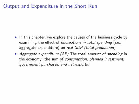
I In this chapter, we explore the causes of the business cycle byexamining the effect of fluctuations in total spending (i.e.,aggregate expenditure) on real GDP (total production).

I Aggregate expenditure (AE) The total amount of spending inthe economy: the sum of consumption, planned investment,government purchases, and net exports.

I (Cont.) During some years, AE increases about as much asdoes the production of goods and services:

I Most firms sell about what they expected to sell and they willremain production and employment unchanged.

I During other years, AE increases more than the production:I Firms will increase production and hire more workers.

I However, during some year, AE didn’t increase as much astotal production:

I Firms cut back on production and laid off workers.

The Aggregate Expenditure Model?

I Aggregate expenditure model A macroeconomic model thatfocuses on the relationship between total spending and realGDP, assuming the price level is constant.

I It is used to study the business cycle involving the interactionof many economic variables.

I The key idea of AE model: In any particular year, the level ofGDP is determined mainly by the level of AE that have severalcomponents.

I Economists began to study the relationship bw fluctuations inAE and fluctuations in GDP during the Great depression ofthe 1930s:

I In 1936, John M. Keynes systematically analyzed thisrelationship in his famous book (“The general theory ofEmployment, Interest, and Money”) and identified fourcategories of AE that together equal to GDP (these are thesame four categories).

Aggregate Expenditure

IAE = C + I + G +NX (1)

1. Consumption (C ): Spending by HHs on G&S such asfurniture, food, etc.

2. Planned Investment (I ): Planned spending by firms on capitalgoods, such as machinery, buildings, etc. or by HHs on newhouses.

3. Government Purchases (G ): Spending by local, state, andfederal governments on G&S, such as building airport,highway, and salaries of gov. employees.

4. Net Exports (NX ): Spending by foreign firms and hhs onG&S produced in the US minus spending by US firms andHHs on G&S produced in other countries.

The Difference between Planned Investment and ActualInvestment

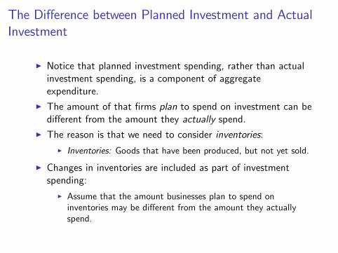
I Notice that planned investment spending, rather than actualinvestment spending, is a component of aggregateexpenditure.

I The amount of that firms plan to spend on investment can bedifferent from the amount they actually spend.

I The reason is that we need to consider inventories:I Inventories: Goods that have been produced, but not yet sold.

I Changes in inventories are included as part of investmentspending:

I Assume that the amount businesses plan to spend oninventories may be different from the amount they actuallyspend.

I (cont.) Changes in inventories depend on sales of goods,which firms cannot always forecast with perfect accuracy.

I E.g., an auto company may produce 15, 000 cars and expect tosell them all. If it does sell all 15, 000, its inventories will beunchanged, but if it sells only 10, 000 it will have an unplannedincrease in inventories.

I Hence, for the economy as a whole, we can say that actualinvestment spending (IS) will be greater (less) than planned ISwhen there is an unplanned increase (decrease) in inventories.

I Actual investment will equal planned investment only whenthere is no unplanned change in inventories.

Macroeconomic Equilibrium

I Macroeconomic equilibrium is similar to microeconomicequilibrium (demand=supply of a product), in which thequantity of apples produced and sold will not change unlessthe demand or supply of this good changes.

I For the economy as a whole, macro equilibrium occurs wheretotal spending equals to total production, that is,

Aggregate Expenditure = GDP

Adjustments to Macro Equilibrium

I Increases and decreases in AE cause the year-to-yearfluctuations in GDP.

I When AE is greater than GDP, inventories will decline, andGDP and total employment will increase.

I When AE is less than GDP, inventories will increase, and GDPand total employment will decrease.

I Only when AE equals GDP will the economy be inmacroeconomic equilibrium.

I Economists forecast what will happen to each component ofAE. If they forecast that AE will decline in the future, that isequivalent to forecasting that GDP will decline and that theeconomy will enter a recession.

I Individuals and firms closely watch these forecasts becausefluctuations in GDP can have dramatic effects on wages,profits, and employment.

I When economists forecast that AE is likely to decline and theeconomy is headed for a recession, the gov. may implementmacro policies to head off the decline in AE and avoid therecession.

10 of 75© 2013 Pearson Education, Inc. Publishing as Prentice Hall

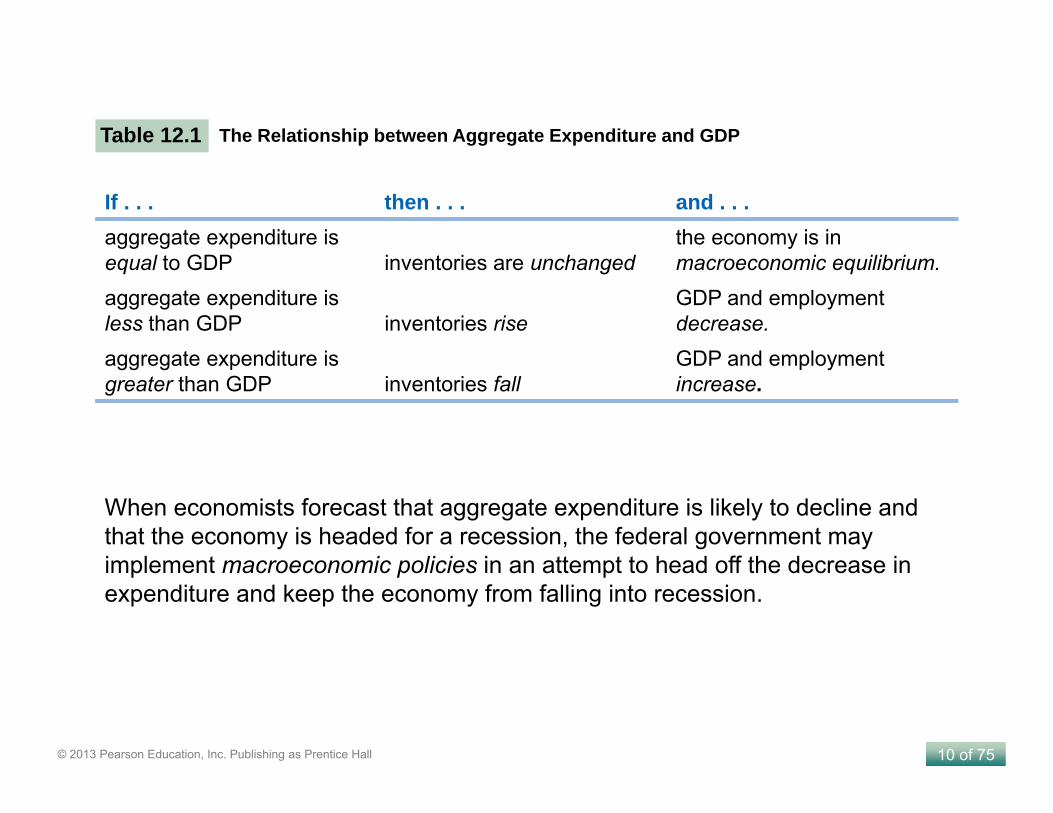
Table 12.1 The Relationship between Aggregate Expenditure and GDP

If . . . then . . . and . . .aggregate expenditure isequal to GDP inventories are unchanged

the economy is inmacroeconomic equilibrium.

aggregate expenditure isless than GDP inventories rise

GDP and employmentdecrease.

aggregate expenditure isgreater than GDP inventories fall

GDP and employmentincrease.

When economists forecast that aggregate expenditure is likely to decline and that the economy is headed for a recession, the federal government may implement macroeconomic policies in an attempt to head off the decrease in expenditure and keep the economy from falling into recession.


Expenditure CategoryReal Expenditure

(billions of 2005 dollars)Consumption $9,221

Planned investment 1,715

Government purchases 2,557

Net exports −422

Table 12.2 Components of Real Aggregate Expenditure, 2010

Each component is measured in real terms, meaning that it is corrected for inflation by being measured in billions of 2005 dollars.

Net exports were negative because in 2010, as in most years since the early 1970s, the United States imported more goods and services than it exported.


Figure 12.1 Real Consumption

Consumption follows a smooth, upward trend, interrupted only infrequently by brief recessions.

Consumption

Consumption

The five most important variables that determine the level ofconsumption:

I Current disposable income is the most important determinantof consumption.

I Disposable income (DI) is the income remaining to HHs afterpaying the personal income tax and receiving gov. transferpayments.

I For most HHs, the higher (lower) their DI, the more (the less)they spend.

I Aggregate (macro) consumption is the total of theconsumption of US HHs. The main reason for the generalupward trend in consumption is that DI has followed a similarupward trend.

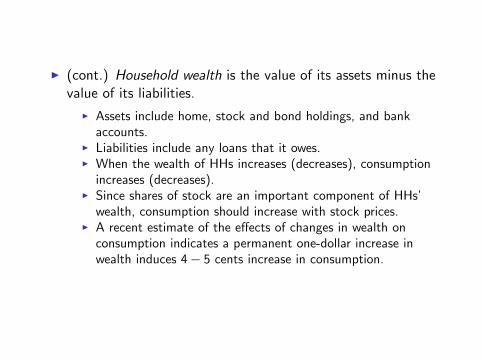
I (cont.) Household wealth is the value of its assets minus thevalue of its liabilities.

I Assets include home, stock and bond holdings, and bankaccounts.

I Liabilities include any loans that it owes.I When the wealth of HHs increases (decreases), consumptionincreases (decreases).

I Since shares of stock are an important component of HHs’wealth, consumption should increase with stock prices.

I A recent estimate of the effects of changes in wealth onconsumption indicates a permanent one-dollar increase inwealth induces 4− 5 cents increase in consumption.

I (cont.) Expected future income: Most people prefer to keeptheir consumption fairly stable and smooth over time, even iftheir income fluctuates significantly. Both current income andexpected future income need to be considered to determinecurrent consumption.

I The price level: Changes in the price level affect consumptionmainly through their effect on HHs’wealth. As the price levelrises, the real value of HHs wealth declines and so will HHsconsumption.

I (cont.) The interest rate: When the interest rate (IR) is high,the reward to saving is increased and HHs are likely to savemore and spend less.

I Note that consumption depends on the real IR that correctsthe nominal IR for the impact of inflation.

I Spending on durable goods (such as autos, one category ofconsumption) is most likely to be affected by the interest ratebecause a high real IR increases the cost of spending financedby borrowing.


Because many macroeconomic variables move together, economists sometimes have difficulty determining whether movements in one are causing movements in another.

Do Changes in Housing Wealth Affect Consumption Spending?

Makingthe

Connection

Your Turn: Test your understanding by doing related problem 2.11 at the end of this chapter.MyEconLab

Housing wealth equals the market value of houses minus the value of loans people have taken out to pay for the houses.

The figure shows the S&P/Case-Shiller index of housing prices, which represents changes in the prices of single-family homes.


Figure 12.2 The Relationship between Consumption and Income, 1960–2010

The Consumption Function

Panel (a) shows the relationship between consumption and income.The points represent combinations of real consumption spending and real disposable income for the years 1960 to 2010. In panel (b), we draw a straight line through the points from panel (a). The line, which represents the relationship between consumption and disposable income, is called the consumption function.The slope of the consumption function is the marginal propensity to consume.

The Consumption Function

I Consumption function The relationship between consumptionspending and disposable income.

I Marginal propensity to consume (MPC): The slope of theconsumption function: the amount by which consumptionspending increases when disposable income increases:

MPC =change in consumption

change in disposable income=

∆C∆YD

. (2)

I We can also use the MPC to determine how muchconsumption will change as income changes:

∆C = MPC × ∆YD.

The Relationship between Consumption and NationalIncome

I Shift to discuss the relationship between aggregateconsumption spending and GDP, rather than disposableincome because we are interested in using the AE model toexplain fluctuations in real GDP.

I Note that GDP and national income are almost the same.I Note that

Disposable income = National income−Net taxes (3)

where Net taxes=taxes minus gov transfer payments. Or,rearranging the equation:

National income = GDP = Disposable income+Net taxes.(4)

Income, Consumption, and Saving

I HHs either (1) spend their income, (2) save it, or (3) use it topay taxes. For the economy as a whole,

National income = Consumption+ Saving+ Taxes, (5)

which means that

Change in national income = Change in consumption (6)

+Change in saving+ Change in taxes

I Using symbols, where Y represents national income (andGDP), C represents consumption, S represents saving, and Trepresents taxes,

Y = C + S + T and ∆Y = ∆C + ∆S + ∆T . (7)


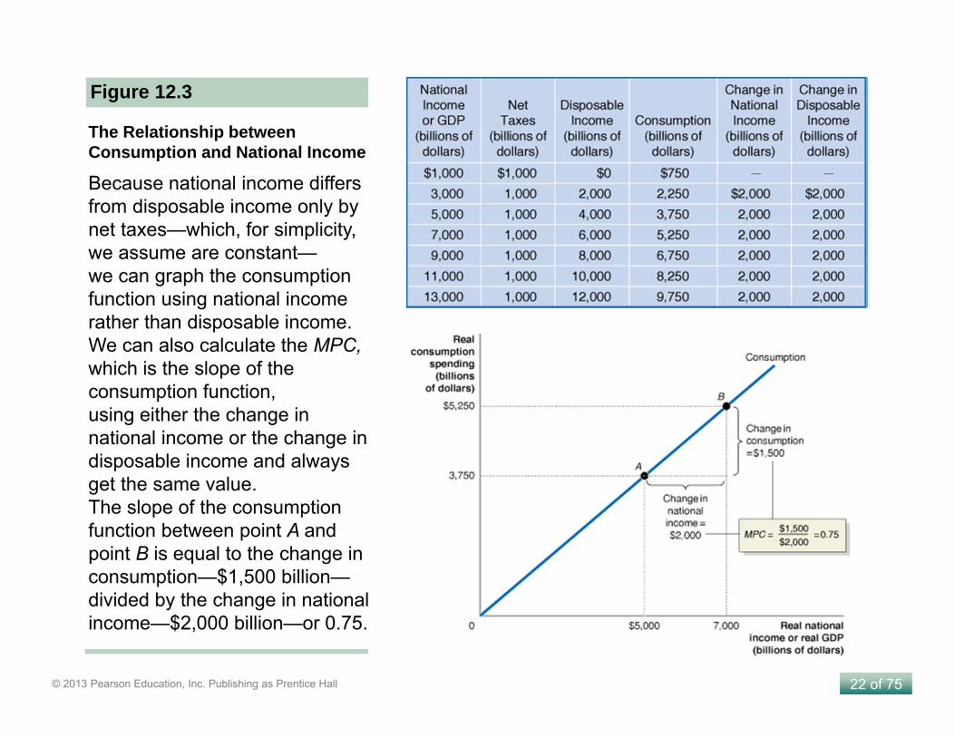
Figure 12.3

The Relationship between Consumption and National Income

Because national income differs from disposable income only by net taxes—which, for simplicity, we assume are constant—we can graph the consumption function using national income rather than disposable income. We can also calculate the MPC,which is the slope of the consumption function, using either the change in national income or the change in disposable income and always get the same value. The slope of the consumption function between point A and point B is equal to the change in consumption—$1,500 billion—divided by the change in national income—$2,000 billion—or 0.75.

I (cont.) To simplify, we can assume that taxes are always aconstant amount, in which case ∆T = 0, so that:

∆Y = ∆C + ∆S .

I Marginal propensity to save (MPS) The change in savingdivided by the change in income:

1 =∆C∆Y

+∆S∆Y

or 1 = MPC +MPS


Calculating the Marginal Propensity to Consume and the Marginal Propensity to Save

Solved Problem 12.2

Step 3: Show that the MPC plus the MPS equals 1.At every level of national income, the MPC is 0.6 and the MPS is 0.4. Therefore, the MPC plus the MPS is always equal to 1.

Your Turn: For more practice, do related problem 2.13 at the end of this chapter.MyEconLab

National Income and Real GDP (Y)

Consumption(C)

Saving(S)

Marginal Propensity to Consume (MPC)

Marginal Propensity to Save (MPS)

$9,000 $8,000 — —

10,000 8,600

11,000 9,200

12,000 9,800

13,000 10,400

$1,000

1,400

1,800

2,200

2,600

0.6 0.4

0.6 0.4

0.6 0.4

Fill in the blanks in the following table. For simplicity, assume that taxes are zero.

Show that the MPC plus the MPS equals 1.

0.6 0.4


Figure 12.4 Real Investment

Planned Investment

Investment is subject to larger changes than is consumption. Investment declined significantly during the recessions of 1980, 1981–1982, 1990–1991, 2001, and 2007–2009.Note: The values are quarterly data, seasonally adjusted at an annual rate.

Planned Investment

I Expectations on future profitabilityI Investment goods (equipment, offi ce buildings) are long-lived.I A firm is unlikely to make a new investment unless it isoptimistic that the demand for its product will remain strongfor several years.

I The optimism or pessimism of firms is an importantdeterminant of investment.

I (cont.)I The interest rate

I Borrowing takes the form of issuing corporate bonds orreceiving loans from banks. A significant fraction ofinvestment is financed by borrowing. HHs also borrow tofinance most of their spending on new houses.

I Because households and firms are interested in the cost ofborrowing after taking into account the effects of inflation,investment spending depends on the real interest rate.

I Holding the other factors that affect investment spendingconstant, there is an inverse relationship between the realinterest rate and investment spending:

I A higher real interest rate results in less investment spending,and a lower real interest rate results in more investmentspending.

I (cont.) TaxesI Firms focus on the profits that remain after paying taxes.I A reduction in the corporate income tax on the profitsincreases the after-tax profitability of investment.

I Investment tax incentives (it provides firms with a taxreduction when they spend on new investment goods) alsoincrease investment spending.

I Cash flowI The difference between the cash revenues received by the firmand the cash spending by the firm.

I Most firms use their own funds to finance investment goodsinstead of borrowing outside.

I The largest contributor to CF is profit. The more profitable afirm is, the greater its CF and the greater its ability to financeinvestment.


Figure 12.5 Real Government Purchases

Government Purchases

Government purchases grew steadily for most of the 1979–2011 period, with the exception of the early 1990s, when concern about the federal budget deficit caused real government purchases to fall for three years, beginning in 1992.Note: The values are quarterly data, seasonally adjusted at an annual rate.

Net Exports

I The price level in US relative to the price levels in othercountries: If prices in US increase more slowly than the pricesof other countries, the demand for US products increasesrelative to other countries.

I The growth rate of GDP in US relative to the growth rates ofother countries: When incomes (GDP) rise faster in US thanin other countries, US consumers’purchases of foreign G&Swill increase faster than foreign consumers’purchases of USG&S.

I The exchange rate between the dollar and other currencies:An increase in the value of the US dollar will reduce exportsand increase imports.


Figure 12.6 Real Net Exports

Net exports were negative in most years between 1979 and 2011. Net exports have usually increased when the U.S. economy is in recession and decreased when the U.S. economy is expanding, although they fell during most of the 2001 recession.Note: The values are quarterly data, seasonally adjusted at an annual rate.

The Important Role of Inventories

I Whenever aggregate expenditure is less than real GDP, somefirms will experience an unplanned increase in inventories.

I If firms don’t cut back on their production promptly, they willaccumulate excess inventories. As a result, even if spendingquickly returns to its normal levels, firms will have to sell theirexcess inventories before they can return to producing atnormal levels.

I This possibility can explain why a brief decline in AE canresult in a fairly long recession. Hence, effi cient systems ofinventories control help make recessions shorter and lesssevere.


Figure 12.7

An Example of a 45°-Line Diagram

The 45° line shows all the points that are equal distances from both axes. Points such as A and B, at which the quantity produced equals the quantity sold, are on the 45° line. Points such as C, at which the quantity sold is greater than the quantity produced, lie above the line. Points such as D, at which the quantity sold is less than the quantity produced, lie below the line.

The 45°-line diagram is sometimes referred to as the Keynesian cross because it is based on the analysis of John Maynard Keynes.


Figure 12.8

The Relationship between Planned Aggregate Expenditure and GDP on a 45°-Line Diagram

Every point of macroeconomic equilibrium is on the 45° line, where planned aggregate expenditure equals GDP. At points above the line, planned aggregate expenditure is greater than GDP. At points below the line, planned aggregate expenditure is less than GDP.

Although all points of macroeconomic equilibrium must lie along the 45° line, only one of these points will represent the actual level of equilibrium real GDP during any particular year, given theactual level of planned real expenditure.

The aggregate expenditure function shows us the amount of planned aggregate expenditure that will occur at every level of national income, or GDP.


Figure 12.9

Macroeconomic Equilibrium on the 45°-Line DiagramMacroeconomic equilibriumoccurs where the aggregateexpenditure (AE) line crosses the 45° line. The lowest upward-sloping line, C, represents the consumption function. The quantities of planned investment, government purchases, and net exports are constant because we assumed that the variables they depend on are constant. So, the total of planned aggregate expenditure at any level of GDP is the amount of consumption at that level of GDP plus the sum of the constant amounts of planned investment, government purchases, and net exports. We successively add each component of spending to the consumption function line to arrive at the line representing aggregate expenditure.


Figure 12.10

Macroeconomic Equilibrium

Macroeconomic equilibrium occurs where the AE line crosses the 45° line. In this case, that occurs at GDP of $10 trillion. If GDP is less than $10 trillion, the corresponding point on the AE line is above the 45° line, planned aggregate expenditure is greater than total production, firms will experience an unplanned decrease in inventories, and GDP will increase. If GDP is greater than $10 trillion, the corresponding point on the AE line is below the 45° line, planned aggregate expenditure is less than total production, firms will experience an unplanned increase in inventories, and GDP will decrease.


Showing a Recession on the 45°-Line Diagram

Macroeconomic equilibrium can occur at any point on the 45° line.

Ideally, we would like equilibrium to occur at potential GDP.

At potential GDP, firms will be operating at their normal level of capacity, and the economy will be at the natural rate of unemployment.

At the natural rate of unemployment, the economy will be at full employment: Everyone in the labor force who wants a job will have one, except the structurally and frictionally unemployed.

For equilibrium to occur at the level of potential GDP, planned aggregate expenditure must be high enough.


Figure 12.11

Showing a Recession on the 45°-Line Diagram

When the aggregate expenditure line intersectsthe 45° line at a level of GDP below potential GDP, the economy is in recession.The figure shows that potential GDP is $10 trillion, but because planned aggregate expenditure is too low, the equilibrium level of GDP is only $9.8 trillion, where the AE line intersects the 45° line. As a result, some firms will be operating below their normal capacity, and unemployment will be above the natural rate of unemployment. We can measure the shortfall in planned aggregate expenditure as the vertical distance between the AE line and the 45° line at the level of potential GDP.


A Numerical Example of Macroeconomic Equilibrium

Real GDP (Y)

Consumption(C)

Planned Investment

(I)


(G)

Net Exports

(NX)

Planned Aggregate

Expenditure(AE)

Unplanned Change in Inventories

Real GDP Will …

$8,000 $6,200 $1,500 $1,500 − $500 $8,700 −$700 increase

9,000 6,850 1,500 1,500 −500 9,350 −350 increase

10,000 7,500 1,500 1,500 −500 10,000 0be in

equilibrium

11,000 8,150 1,500 1,500 −500 10,650 +350 decrease

12,000 8,800 1,500 1,500 −500 11,300 +700 decrease

Note: The values are in billions of 2005 dollars

Table 12.3 Macroeconomic Equilibrium

Don’t Let This Happen to YouDon’t Confuse Aggregate Expenditure with Consumption SpendingPlanned aggregate expenditure equals the sum of consumption spending, planned investment spending, government purchases, and net exports, not consumption spending by itself.


We can capture some key features contained in the quantitative models that economic forecasters use by looking at several hypothetical combinations of real GDP and planned aggregate expenditure.


Determining Macroeconomic EquilibriumSolved Problem 12.3

Fill in the blanks in the following table and determine the equilibrium level of real GDP.

To fill in the first row, we have AE = $6,200 billion + $1,675 billion + $1,675 billion + (−$500 billion) = $9,050 billion; and unplanned change in inventories = $8,000 billion − $9,050 billion = −$1,050 billion.

Step 3: Determine the equilibrium level of real GDP.Once you fill in the table, you should see that equilibrium real GDP must be $11,000 billion because only at that level is real GDP equal to planned aggregate expenditure.

Your Turn: For more practice, do related problem 3.12 at the end of this chapter.MyEconLab

Real GDP (Y)

Consumption(C)

Planned Investment

(I)


(G)

Net Exports

(NX)

Planned Aggregate

Expenditure(AE)

Unplanned Change in Inventories

$8,000 $6,200 $1,675 $1,675 $−500

9,000 6,850 1,675 1,675 −500

10,000 7,500 1,675 1,675 −500

11,000 8,150 1,675 1,675 −500

12,000 8,800 1,675 1,675 −500Note: The values are in billions of 2005 dollars.

$9,050 $−1,050

9,700

10,350

11,000

11,650

−700

−350

0

350

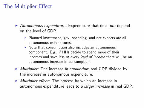
The Multiplier Effect

I Autonomous expenditure: Expenditure that does not dependon the level of GDP.

I Planned investment, gov. spending, and net exports are allautonomous expenditures.

I Note that consumption also includes an autonomouscomponent. E.g., if HHs decide to spend more of theirincomes and save less at every level of income there will be anautonomous increase in consumption.

I Multiplier: The increase in equilibrium real GDP divided bythe increase in autonomous expenditure.

I Multiplier effect: The process by which an increase inautonomous expenditure leads to a larger increase in real GDP.


Figure 12.12

The Multiplier Effect

The economy begins at point A, at which equilibrium real GDP is $9.6 trillion. A $100 billion increase in planned investment shifts up aggregate expenditure from AE1 to AE2. The new equilibrium is at point B, where real GDP is $10.0 trillion, which is potential real GDP. Because of the multiplier effect, a $100 billion increase in investment results in a $400 billion increase in equilibrium real GDP.

A Formula for the Multiplier

I

The total change in GDP = $100+MPC × $100(8)

+MPC ×MPC × $100+ . . . =⇒ 11−MPC .

I

Multiplier =Change in real GDP

Change in autonomous expenditure=

11−MPC .

(9)


Table 12.4 The Multiplier Effect in Action

Additional Autonomous Expenditure (investment)

Additional Induced Expenditure

(consumption)

Total Additional Expenditure =

Total Additional GDPRound 1 $100 billion $0 $100 billionRound 2 0 75 billion 175 billionRound 3 0 56 billion 231 billionRound 4 0 42 billion 273 billionRound 5 0 32 billion 305 billion...

.

.

.

.

.

.

.

.

.Round 10 0 8 billion 377 billion...

.

.

.

.

.

.

.

.


.

.

.

.

.

.

.

.


.

.

.

.

.

.

.

.

.Round n 0 0 $400 billion

By thinking of the multiplier effect occurring in rounds of spending, we can summarize how changes in GDP and spending caused by the initial $100 billion increase in investment will result in equilibrium GDP rising by $400 billion.


Year Consumption Investment Net Exports Real GDP Unemployment Rate1929 $737 billion $102 billion −$11 billion $977 billion 3.2%

1933 $601 billion $19 billion −$12 billion $716 billion 24.9%Note: The values are in 2005 dollars.

The Multiplier in Reverse: The Great Depression of the 1930s

Makingthe

ConnectionAn increase in autonomous expenditure causes an increase in equilibrium real GDP, but the reverse is also true: A decrease in autonomous expenditure causes a decrease in real GDP.

Americans became aware of this fact in the 1930s when the multiplier effect magnified reductions in autonomous expenditure, leading to very high levels of unemployment and the largest decline in real GDP in U.S. history.

The following table shows the severity of the economic downturn by contrasting the business cycle peak of 1929 with the business cycle trough of 1933:


The Multiplier in Reverse: The Great Depression of the 1930s

Makingthe

Connection


We can use a 45°-line diagram to illustrate the multiplier effect working in reverse during these years.

The economy was at potential real GDP in 1929, before the declines in aggregate expenditure began.

Declining consumption, planned investment, and net exports shifted the aggregate expenditure function down from AE1929 to AE1933, reducing equilibrium real GDP from $977 billion in 1929 to $716 billion in 1933.

The depth and length of this economic downturn led to its being labeled the Great Depression.

Summarizing the Multiplier EffectI The multiplier effect occurs both when autonomousexpenditure increases and when it decreases.

I For example, with an MPC of 0.75, a decrease in plannedinvestment of $100 billion will lead to a decrease in equilibriumincome of $400 billion.

I The multiplier effect makes the economy more sensitive tochanges in autonomous expenditure than it would otherwisebe.

I Because of the multiplier effect, a decline in spending andproduction in one sector of the economy can lead to declines inspending and production in many other sectors of the economy.

I The larger the MPC, the larger the value of the multiplier.I The formula for the multiplier, 1

1−MPC , is oversimplifiedbecause it ignores some real world complications, such as theeffect that an increasing GDP can have on imports, inflation,and interest rates. These effects combine to cause the simpleformula to overstate the true value of the multiplier.


Using the Multiplier FormulaSolved Problem 12.4

Step 2: Determine equilibrium real GDP.Just as in Solved Problem 12.2, we can find macroeconomic equilibrium by calculating the level of planned aggregate expenditure for each level of real GDP.We can see that macroeconomic equilibrium will occur when real GDP equals $10,000 billion.

Step 3: Calculate the MPC.YCMPC

ΔΔ

=

In this case: 8.0billion $1,000

billion $800==MPC

Use the information in the table to answer the following questions:

Real GDP (Y)

Consumption(C)

Planned Investment

(I)


(G)Net Exports

(NX)$8,000 $6,900 $1,000 $1,000 −$500

9,000 7,700 1,000 1,000 −500

10,000 8,500 1,000 1,000 −500

11,000 9,300 1,000 1,000 −500

12,000 10,100 1,000 1,000 −500

Note: The values are in billions of 2005 dollars.

Planned Aggregate

Expenditure(AE)

$8,400

9,200

10,000

10,800

11,600


Using the Multiplier FormulaSolved Problem 12.4

So:

Change in equilibrium real GDP = Change in autonomous expenditure × 5

Or:

Change in equilibrium real GDP = $200 billion × 5 = $1,000 billion

Therefore:

New level of equilibrium GDP = $10,000 billion + $1,000 billion= $11,000 billion


Step 4: Use the multiplier formula to calculate the new equilibrium level of real GDP.We could find the new level of equilibrium real GDP by constructing a new table with government purchases increased from $1,000 billion to $1,200 billion. But the multiplier allows us to calculate the answer directly. In this case:

58.01

11

1Multiplier =−

=−

=MPC

The Paradox of Thrift

I In discussing the AE model, John Maynard Keynes arguedthat if many households decide at the same time to increasetheir saving and reduce their spending, they may makethemselves worse off by causing aggregate expenditure to fall,thereby pushing the economy into a recession.

I The lower incomes in the recession might mean that totalsaving does not increase, despite the attempts by manyindividuals to increase their own saving.

I Keynes referred to this outcome as the paradox of thriftbecause what appears to be something favorable to thelong-run performance of the economy might becounterproductive in the short run.

The Aggregate Demand Curve

I When demand for a product increases, firms will usuallyrespond by increasing production, but they are also likely toincrease prices. So far, we have fixed the price level (PL).

I In fact, as we will see, increases (decreases) in the PL willcause AE decrease (rise). There are 3 reasons for this inverserelationship between changes in the PL and changes in AE.

(cont.)

I 1. A rising PL decreases consumption by decreasing the real valueof household wealth.

2. If the PL in US rises relative to the PLs in other countries, USexports will become relatively more expensive and foreignimports will become relatively less expensive, causing netexports to fall.

3. When prices rise, firms and HHs need more money to financebuying and selling. If the central bank doesn’t increase moneysupply, the result will increase the IR and then reduceinvestment as firms and HHs borrow less to build newfactories, ect., and new houses, respectively.

I Aggregate demand curve (AD) A curve showing therelationship between the price level and the level of plannedaggregate expenditure in the economy, holding constant allother factors that affect aggregate expenditure.


Figure 12.13 The Effect of a Change in the Price Level on Real GDP

In panel (a), an increase in the price level results in declining consumption, planned investment, and net exports and causes the aggregate expenditure line to shift down from AE1 to AE2.As a result, equilibrium real GDP declines from $10.0 trillion to $9.8 trillion.In panel (b), a decrease in the price level results in rising consumption, planned investment, and net exports and causes the aggregate expenditure line to shift up from AE1 to AE2.As a result, equilibrium real GDP increases from $10.0 trillion to $10.2 trillion.


The Algebra of Macroeconomic Equilibrium

Appendix

Apply the algebra of macroeconomic equilibrium.LEARNING OBJECTIVE

Graphs help us understand economic change qualitatively.

When we write an economic model using equations, we make it easier to make quantitative estimates.

An econometric model is an economic model written in the form of equations, where each equation has been statistically estimated, using methods similar to the methods used in estimating demand curves.


The following equations are based on the example shown in Table 12.3. Y stands for real GDP, and the numbers (with the exception of the MPC) represent billions of dollars.

1. C = 1,000 + 0.65Y

2. I = 1,500

3. G = 1,500

4. NX = −500

5. Y = C + I + G + NX

Consumption function

Planned investment function

Government spending function

Net export function

Equilibrium condition

The parameters of the functions—such as the value of autonomous consumption and the value of the MPC in the consumption function—would be estimated statistically, using data on the values of each variable overa period of years.


In this model, GDP is in equilibrium when it equals planned aggregate expenditure.

Equation 5—the equilibrium condition—shows us how to calculate equilibrium in the model: We need to substitute equations 1 through 4 into equation 5.Doing so gives us the following:

Y = 1,000 + 0.65Y + 1,500 + 1,500 − 500

We need to solve this expression for Y to find equilibrium GDP. The first step is to subtract 0.65Y from both sides of the equation:

Y − 0.65Y = 1,000 + 1,500 + 1,500 − 500

Then, we solve for Y:

0.35Y = 3,500

Or:

000,1035.0

500,3==Y


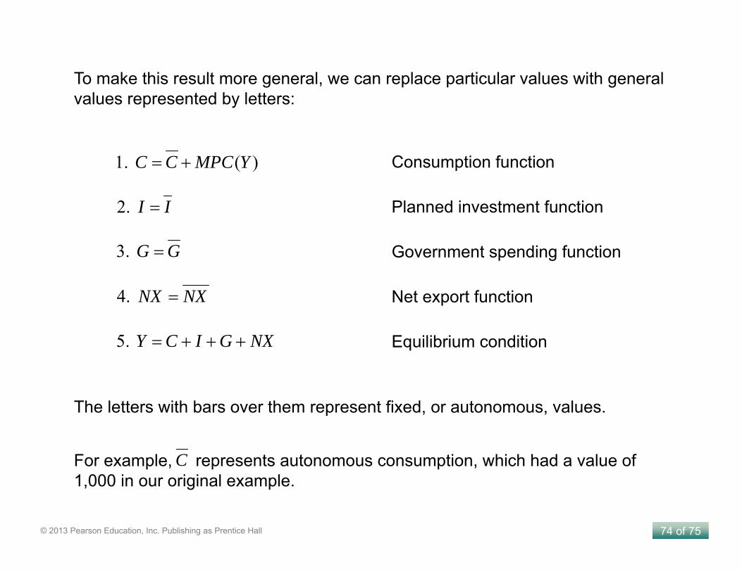
To make this result more general, we can replace particular values with general values represented by letters:

)( 1. YMPCCC +=

II 2. =

GG 3. =

NXNX 4. =

NXGICY +++= 5.

Consumption function

Planned investment function

Government spending function

Net export function

Equilibrium condition

For example, represents autonomous consumption, which had a value of 1,000 in our original example.

C

The letters with bars over them represent fixed, or autonomous, values.


Solving now for equilibrium, we get

NXGIYMPCCY ++++= )(

NXGICYMPCY +++=− )(

or

or

NXGICMPCY +++=− )1(

or

MPCNXGICY

−+++

=1

Remember that 1/(1 − MPC) is the multiplier, and all four variables in the numerator of the equation represent autonomous expenditure. Therefore, an alternative expression for equilibrium GDP is:

Equilibrium GDP = Autonomous expenditure × Multiplier


Figure 12.14

The Aggregate Demand Curve

The aggregate demand (AD) curve shows the relationship between the price level and the level of planned aggregate expenditure in the economy. When the price level is 97,real GDP is $10.2 trillion. An increase in the price level to 100 causes consumption, investment, and net exports to fall,which reduces real GDP to $10.0 trillion.

Aggregate demand (AD) curve A curve that shows the relationship between the price level and the level of planned aggregate expenditure in the economy, holding constant all other factors that affect aggregate expenditure.

chapter 12: aggregate expenditure and output in the …yluo/teaching/econ1002cd/chapter12.… ·...

Documents