chapter 11 lasers - ugentphotonics.intec.ugent.be/education/ivpv/res_handbook/v1ch11.pdf · chapter...
TRANSCRIPT

CHAPTER 11 LASERS
William T . Silfvast Center for Research and Education in Optics and Lasers ( CREOL ) Uni y ersity of Central Florida Orlando , Florida
1 1 . 1 GLOSSARY
A 2 radiative transition probability from level 2 to all other possible lower-lying levels
A 2 1 radiative transition probability from level 2 to level 1
a L scattering losses within a laser cavity for a single pass through the cavity
B 1 2 Einstein B coef ficient associated with absorption
B 2 1 Einstein B coef ficient associated with stimulated emission
E 1 , E 2 energies of levels 1 and 2 above the ground state energy for that species
g 1 , g 2 stability parameters for laser modes when describing the laser optical cavity
g 1 , g 2 statistical weights of energy levels 1 and 2 that indicate the degeneracy of the levels
g 2 1 gain coef ficient for amplification of radiation within a medium at a wavelength of l 2 1
I s a t saturation intensity of a beam in a medium ; intensity at which exponential growth will cease to occur even though the medium has uniform gain (energy / time-area)
N 1 , N 2 population densities (number of species per unit volume) in energy levels 1 and 2
r c radius of curvature of the expanding wavefront of a gaussian beam
R 1 , R 2 reflectivities of mirrors 1 and 2 at the desired wavelength
T 1 lifetime of a level when dominated by collisional decay
T 2 average time between phase-interrupting collisions of a species in a specific excited state
t o p t optimum mirror transmission for a laser of a given gain and loss
11 .1

11 .2 OPTICAL SOURCES
w ( z ) beam waist at a distance z from the minimum beam waist for a gaussian beam
w o minimum beam waist radius for a gaussian mode
a 1 2 absorption coef ficient for absorption of radiation within a medium at wavelength l 2 1
g 2 1 angular frequency bandwidth of an emission or absorption line
D t p pulse duration of a mode-locked laser pulse
D … frequency bandwidth over which emission , absorption , or amplification can occur
D … D frequency bandwidth (FWHM) when the dominant broadening process is Doppler or motional broadening
h index of refraction of the laser medium at the desired wavelength
l 2 1 wavelength of a radiative transition occurring between energy levels 2 and 1
… 2 1 frequency of a radiative transition occurring between energy levels 2 and 1
s 2 1 stimulated emission cross section (area)
s D 21 stimulated emission cross section at line center when Doppler broadening
dominates (area)
s H 21 stimulated emission cross section at line center when homogeneous broaden-
ing dominates (area)
τ 2 lifetime of energy level 2
τ 2 1 lifetime of energy level 2 if it can only decay to level 1
1 1 . 2 INTRODUCTION
A laser is a device that amplifies light and produces a highly directional , high-intensity beam that typically has a very pure frequency or wavelength . It comes in sizes ranging from approximately one-tenth the diameter of a human hair to the size of a very large building , in powers ranging from 10 2 9 to 10 2 0 watts , and in wavelengths ranging from the microwave to the soft-x-ray spectral regions with corresponding frequencies from 10 1 1 to 10 1 7 Hz . Lasers have pulse energies as high as 10 4 joules and pulse durations as short as 6 3 10 2 1 5 seconds . They can easily drill holes in the most durable of materials and can weld detached retinas within the human eye .
Lasers are a key component of some of our most modern communication systems and are the ‘‘phonograph needle’’ of compact disc players . They are used for heat treatment of high-strength materials , such as the pistons of automobile engines , and provide a special surgical knife for many types of medical procedures . They act as target designators for military weapons and are used in the checkout scanners we see everyday at the supermarket .
The word laser is an acronym for L ight A mplification by S timulated E mission of R adiation . The laser makes use of processes that increase or amplify light signals after those signals have been generated by other means . These processes include (1) stimulated emission , a natural ef fect that arises out of considerations relating to thermodynamic

LASERS 11 .3
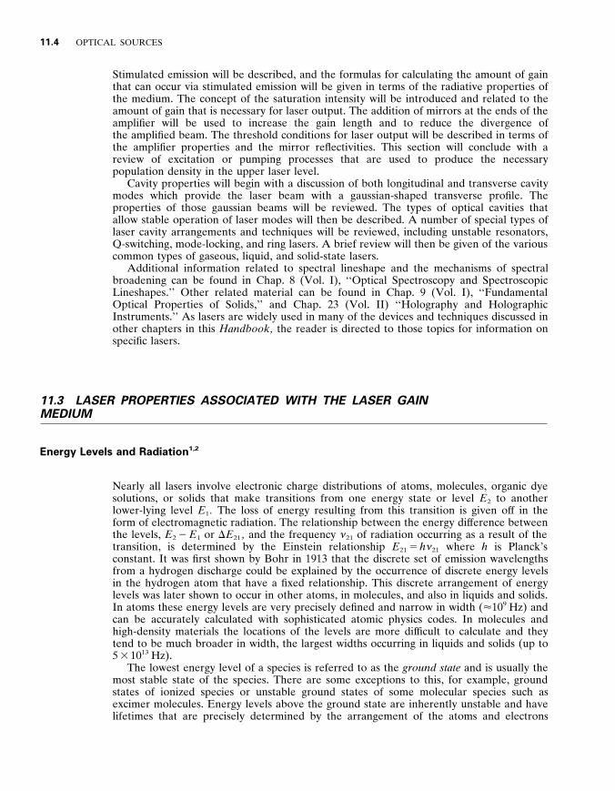
FIGURE 1 Simplified diagram of a laser , including the amplifying medium and the optical resonator .
equilibrium , and (2) optical feedback (present in most lasers) that is usually provided by mirrors . Thus , in its simplest form , a laser consists of a gain or amplifying medium (where stimulated emission occurs) and a set of mirrors to feed the light back into the amplifier for continued growth of the developing beam (Fig . 1) .
The entire spectrum of electromagnetic radiation is shown in Fig . 2 , along with the region covered by currently existing lasers . Such lasers span the wavelength range from the far infrared part of the spectrum ( l 5 1000 m m) to the soft-x-ray region ( l 5 3 nm) , thereby covering a range of almost six orders of magnitude! There are several types of units that are used to define laser wavelengths . These range from micrometers ( m m) in the infrared to nanometers (nm) and angstroms ( Å ) in the visible , ultraviolet (UV) , vacuum ultraviolet (VUV) , extreme ultraviolet (EUV or XUV) , and soft-x-ray (SXR) spectral regions .
This chapter provides a brief overview of how a laser operates . It considers a laser as having two primary components : (1) a region where light amplification occurs which is referred to as a gain medium or an amplifier , and (2) a ca y ity , which generally consists of two mirrors placed at either end of the amplifier .
Properties of the amplifier include the concept of discrete excited energy levels and their associated finite lifetimes . The broadening of these energy levels will be associated with the emission linewidth which is related to decay of the population in these levels .
FIGURE 2 The portion of the electromagnetic spectrum that involves lasers , along with the general wavelengths of operation of most of the common lasers .
11 .4 OPTICAL SOURCES
Stimulated emission will be described , and the formulas for calculating the amount of gain that can occur via stimulated emission will be given in terms of the radiative properties of the medium . The concept of the saturation intensity will be introduced and related to the amount of gain that is necessary for laser output . The addition of mirrors at the ends of the amplifier will be used to increase the gain length and to reduce the divergence of the amplified beam . The threshold conditions for laser output will be described in terms of the amplifier properties and the mirror reflectivities . This section will conclude with a review of excitation or pumping processes that are used to produce the necessary population density in the upper laser level .
Cavity properties will begin with a discussion of both longitudinal and transverse cavity modes which provide the laser beam with a gaussian-shaped transverse profile . The properties of those gaussian beams will be reviewed . The types of optical cavities that allow stable operation of laser modes will then be described . A number of special types of laser cavity arrangements and techniques will be reviewed , including unstable resonators , Q-switching , mode-locking , and ring lasers . A brief review will then be given of the various common types of gaseous , liquid , and solid-state lasers .
Additional information related to spectral lineshape and the mechanisms of spectral broadening can be found in Chap . 8 (Vol . I) , ‘‘Optical Spectroscopy and Spectroscopic Lineshapes . ’’ Other related material can be found in Chap . 9 (Vol . I) , ‘‘Fundamental Optical Properties of Solids , ’’ and Chap . 23 (Vol . II) ‘‘Holography and Holographic Instruments . ’’ As lasers are widely used in many of the devices and techniques discussed in other chapters in this Handbook , the reader is directed to those topics for information on specific lasers .
1 1 . 3 LASER PROPERTIES ASSOCIATED WITH THE LASER GAIN MEDIUM
Energy Levels and Radiation 1 , 2
Nearly all lasers involve electronic charge distributions of atoms , molecules , organic dye solutions , or solids that make transitions from one energy state or level E 2 to another lower-lying level E 1 . The loss of energy resulting from this transition is given of f in the form of electromagnetic radiation . The relationship between the energy dif ference between the levels , E 2 2 E 1 or D E 2 1 , and the frequency … 2 1 of radiation occurring as a result of the transition , is determined by the Einstein relationship E 2 1 5 h … 2 1 where h is Planck’s constant . It was first shown by Bohr in 1913 that the discrete set of emission wavelengths from a hydrogen discharge could be explained by the occurrence of discrete energy levels in the hydrogen atom that have a fixed relationship . This discrete arrangement of energy levels was later shown to occur in other atoms , in molecules , and also in liquids and solids . In atoms these energy levels are very precisely defined and narrow in width ( < 10 9 Hz) and can be accurately calculated with sophisticated atomic physics codes . In molecules and high-density materials the locations of the levels are more dif ficult to calculate and they tend to be much broader in width , the largest widths occurring in liquids and solids (up to 5 3 10 1 3 Hz) .
The lowest energy level of a species is referred to as the ground state and is usually the most stable state of the species . There are some exceptions to this , for example , ground states of ionized species or unstable ground states of some molecular species such as excimer molecules . Energy levels above the ground state are inherently unstable and have lifetimes that are precisely determined by the arrangement of the atoms and electrons
LASERS 11 .5
associated with any particular level as well as to the particular species or material . Thus , when an excited state is produced by applying energy to the system , that state will eventually decay by emitting radiation over a time period ranging from 10 2 1 5 seconds or less to times as long as seconds or more , depending upon the particular state or level involved . For strongly allowed transitions that involve the electron charge cloud changing from an atomic energy level of energy E 2 to a lower-lying level of energy E 1 , the radiative decay time τ 2 1 can be approximated by τ 2 1 < 10 4 l 2
21 where τ 2 1 is in seconds and l 2 1 is the wavelength of the emitted radiation in meters . l 2 1 is related to … 2 1 by the relationship l 2 1 … 2 1 5 c / h where c is the velocity of light (3 3 10 8 m / sec) and h is the index of refraction of the material . For most gases , h is near unity and for solids and liquids it ranges between 1 and 10 , with most values ranging from < 1 . 3 – 2 . 0 .
Using the expression suggested above for the approximate value of the lifetime of an excited energy level , one obtains a decay time of several nsec for green light ( l 2 1 5 5 3 10 2 7 m) . This represents a minimum radiative lifetime since most excited energy levels have a weaker radiative decay probability than mentioned above and would therefore have radiative lifetimes one or two orders of magnitude longer . Other laser materials such as molecules , organic dye solutions , and semiconductor lasers have similar radiative lifetimes . The one exception is the class of dielectric solid-state laser materials (both crystalline and glass) such as ruby and Nd : YAG , in which the lifetimes are of the order of 1 – 300 m sec . This much longer radiative lifetime in solid-state laser materials is due to the nature of the particular state of the laser species and to the crystal matrix in which it is contained . This is a very desirable property for a laser medium since it allows excitation and energy storage within the laser medium over a relatively long period of time .
Emission Linewidth and Line Broadening of Radiating Species 1 , 3
Assume that population in energy level 2 decays to energy level 1 with an exponential decay time of τ 2 1 and emits radiation at frequency … 2 1 during that decay . It can be shown by Fourier analysis that the exponential decay of that radiation requires the frequency width of the emission to be of the order of D … > 1 / 2 π τ 2 1 . This suggests that the energy width D E 2 of level 2 is of the order of D E 2 5 h / 2 π τ 2 1 . If the energy level 2 can decay to more levels than level 1 , with a corresponding decay time of τ 2 , then its energy is broadened by an amount D E 2 5 h / 2 π τ 2 . If the decay is due primarily to radiation at a rate A 2 i to one or more individual lower-lying levels i , then 1 / τ 2 5 A 2 5 o
i A 2 i . A 2 represents the
total radiative decay rate of level 2 , whereas A 2 i is the specific radiative decay rate from level 2 to a lower-lying level i .
If population in level 2 decays radiatively at a radiative rate A 2 and population in level 1 decays radiatively at a rate A 1 , then the emission linewidth of radiation from level 2 to 1 is given by
D … 2 1 5
O i
A 2 i 1 O j
A 1 j
2 π (1)
which is referred to as the natural linewidth of the transition and represents the sum of the widths of levels 2 and 1 in frequency units . If , in the above example , level 1 is a ground state with infinite lifetime or a long-lived metastable level , then the natural linewidth of the emission from level 2 to level 1 would be represented by
D … 2 1 5
O i
A 2 i
2 π (2)
11 .6 OPTICAL SOURCES
since the ground state would have an infinite lifetime and would therefore not contribute to the broadening . This type of linewidth or broadening is known as natural broadening since it results specifically from the radiative decay of a species . Thus the natural linewidth associated with a specific transition between two levels has an inherent value determined only by the factors associated with specific atomic and electronic characteristics of those levels .
The emission-line broadening or natural broadening described above is the minimum line broadening that can occur for a specific radiative transition . There are a number of mechanisms that can increase the emission linewidth . These include collisional broadening , phase-interruption broadening , Doppler broadening , and isotope broadening . The first two of these , along with natural broadening , are all referred to as homogeneous broadening . Homogeneous broadening is a type of emission broadening in which all of the atoms radiating from the specific level under consideration participate in the same way . In other words , all of the atoms have the identical opportunity to radiate with equal probability .
The type of broadening associated with either Doppler or isotope broadening is referred to as inhomogeneous broadening . For this type of broadening , only certain atoms radiating from that level that have a specific property such as a specific velocity , or are of a specific isotope , participate in radiation at a certain frequency within the emission bandwidth .
Collisional broadening is a type of broadening that is produced when surrounding atoms , molecules , solvents (in the case of dye lasers) , or crystal structures interact with the radiating level and cause the population to decay before it has a chance to decay by its normal radiative processes . The emission broadening is then associated with the faster decay time T 1 , or D … 5 1 / 2 π T 1 .
Phase - interruption broadening or phonon broadening is a type of broadening that does not increase the decay rate of the level , but it does interrupt the phase of the rotating electron cloud on average over a time interval T 2 which is much shorter than the radiative decay time τ 2 which includes all possible radiative decay channels from level 2 . The result of this phase interruption is to increase the emission linewidth beyond that of both natural broadening and T 1 broadening (if it exists) to an amount D … 5 1 / 2 π T 2 .
Doppler broadening is a type of inhomogeneous broadening in which the Doppler ef fect shifts the frequencies of atoms moving toward the observer to a higher value and the frequencies of atoms moving away from the observer to a lower value . This ef fect occurs only in gases since they are the only species that are moving fast enough to produce such broadening . Doppler broadening is the dominant broadening process in most visible gas lasers . The expression for the Doppler linewidth (FWHM) is given by
D … D 5 7 . 16 ? 10 2 7 … o – T
M (3)
in which … o is the center frequency associated with atoms that are not moving either toward or away from the observer , T is the gas temperature in kelvin and M is the atomic or molecular weight (number of nucleons / atom or molecule) of the gas atoms or molecules .
Isotope broadening also occurs in some gas lasers . It becomes the dominant broadening process if the specific gas consists of several isotopes of the species and if the isotope shifts for the specific radiative transition are broader than the Doppler width of the transition . The helium-cadmium laser is dominated more by this ef fect than any other laser since the naturally occurring cadmium isotopic mixture contains eight dif ferent isotopes and the isotope shift between adjacent isotopes (adjacent neutron numbers) is approximately equal to the Doppler width of the individual radiating isotopes . This broadening ef fect can be eliminated by the use of isotopically pure individual isotopes , but the cost for such isotopes is often prohibitive .
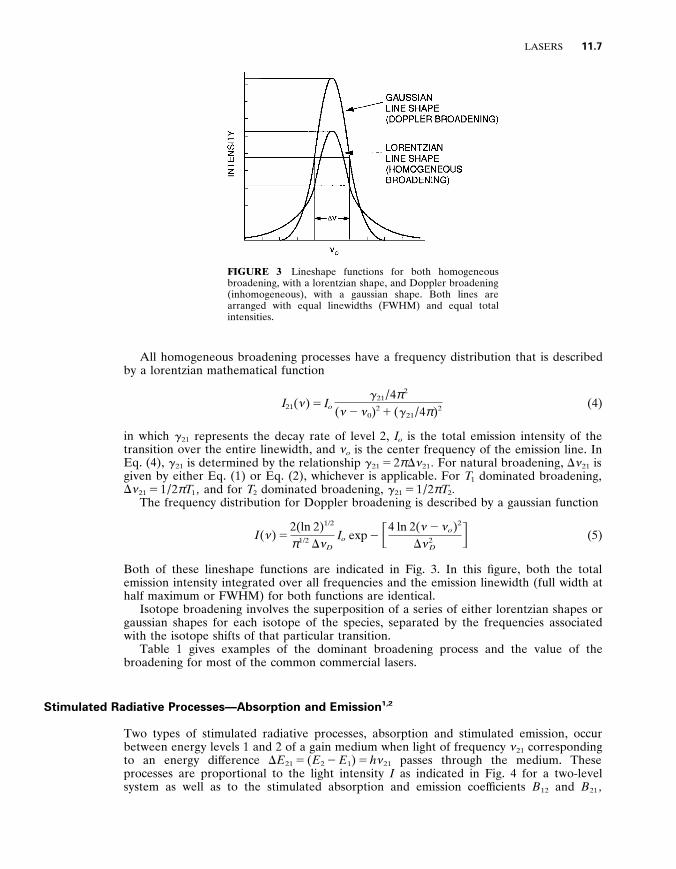
LASERS 11 .7
FIGURE 3 Lineshape functions for both homogeneous broadening , with a lorentzian shape , and Doppler broadening (inhomogeneous) , with a gaussian shape . Both lines are arranged with equal linewidths (FWHM) and equal total intensities .
All homogeneous broadening processes have a frequency distribution that is described by a lorentzian mathematical function
I 2 1 ( … ) 5 I o g 2 1 / 4 π 2
( … 2 … 0 ) 2 1 ( g 2 1 / 4 π ) 2 (4)
in which g 2 1 represents the decay rate of level 2 , I o is the total emission intensity of the transition over the entire linewidth , and … o is the center frequency of the emission line . In Eq . (4) , g 2 1 is determined by the relationship g 2 1 5 2 π D … 2 1 . For natural broadening , D … 2 1 is given by either Eq . (1) or Eq . (2) , whichever is applicable . For T 1 dominated broadening , D … 2 1 5 1 / 2 π T 1 , and for T 2 dominated broadening , g 2 1 5 1 / 2 π T 2 .
The frequency distribution for Doppler broadening is described by a gaussian function
I ( … ) 5 2(ln 2) 1 / 2
π 1 / 2 D … D I o exp 2 F 4 ln 2( … 2 … o ) 2
D … 2 D
G (5)
Both of these lineshape functions are indicated in Fig . 3 . In this figure , both the total emission intensity integrated over all frequencies and the emission linewidth (full width at half maximum or FWHM) for both functions are identical .
Isotope broadening involves the superposition of a series of either lorentzian shapes or gaussian shapes for each isotope of the species , separated by the frequencies associated with the isotope shifts of that particular transition .
Table 1 gives examples of the dominant broadening process and the value of the broadening for most of the common commercial lasers .
Stimulated Radiative Processes—Absorption and Emission 1 , 2
Two types of stimulated radiative processes , absorption and stimulated emission , occur between energy levels 1 and 2 of a gain medium when light of frequency … 2 1 corresponding to an energy dif ference D E 2 1 5 ( E 2 2 E 1 ) 5 h … 2 1 passes through the medium . These processes are proportional to the light intensity I as indicated in Fig . 4 for a two-level system as well as to the stimulated absorption and emission coef ficients B 1 2 and B 2 1 ,

11 .8 OPTICAL SOURCES
TABLE 1 Amplifier Parameters for a Wide Range of Lasers
respectively . These coef ficients are related to the frequency … 2 1 and the spontaneous emission probability A 2 1 associated with the two levels . A 2 1 has units of (1 / sec) .
Absorption results in the loss of light of intensity I when the light interacts with the medium . The energy is transferred from the beam to the medium by raising population from level 1 to the higher-energy level 2 . In this situation , the species within the medium can either reradiate the energy and return to its initial level 1 , it can reradiate a dif ferent energy and decay to a dif ferent level , or it can lose the energy to the surrounding medium via collisions , which results in the heating of the medium , and return to the lower level . The absorption probability is proportional to the intensity I which has units of energy / sec-m 2 times B 1 2 , which is the absorption probability coef ficient for that transition . B 1 2 is one of the Einstein B coef ficients and has the units of m 3 / energy-sec 2 .
Stimulated emission results in the increase in the light intensity I when light of the appropriate frequency … 2 1 interacts with population occupying level 2 of the gain medium . The energy is given up by the species to the radiation field . In the case of stimulated
FIGURE 4 Stimulated emission and absorption processes that can occur between two energy levels , 1 and 2 , and can significantly alter the population densities of the levels compared to when a beam of intensity I is not present .

LASERS 11 .9
emission , the emitted photons or bundles of light have exactly the same frequency … 2 1 and direction as the incident photons of intensity I that produce the stimulation . B 2 1 is the associated stimulated emission coef ficient and has the same units as B 1 2 . It is known as the other Einstein B coef ficient .
Einstein showed the relationship between B 1 2 , B 2 1 , and A 2 1 as
g 2 B 2 1 5 g 1 B 1 2 (6)
and
A 2 1 5 8 π h … 3
21
c 3 B 2 1 (7)
where g 2 and g 1 are the statistical weights of levels 2 and 1 and h is Planck’s constant . Since A 2 1 5 1 / τ 2 1 for the case where radiative decay dominates and where there is only one decay path from level 2 , B 2 1 can be determined from lifetime measurements or from absorption measurements on the transition at frequency … 2 1 .
Population Inversions 1 ,2
The two processes of absorption and stimulated emission are the principal interactions involved in a laser amplifier . Assume that a collection of atoms of a particular species is energized to populate two excited states 1 and 2 with population densities N 1 and N 2 (number of species / m 3 ) and state 2 is at a higher energy than state 1 by an amount D E 2 1 as described in the previous section . If a photon beam of energy D E 2 1 , with an intensity I o and a corresponding wavelength l 2 1 5 c / … 2 1 5 hc / D E 2 1 , passes through this collection of atoms , then the intensity I after the beam emerges from the medium can be expressed as
I 5 I o e s 2 1 ( N 2 2 ( g 2 / g 1 ) N 1 ) L 5 I o e s 2 1 D N 2 1 L (8)
where s 2 1 is referred to as the stimulated emission cross section with dimensions of m 2 , L is the thickness of the medium (in meters) through which the beam passes , and N 2 2 ( g 2 / g 1 ) N 1 5 D N 2 1 is known as the population in y ersion density . The exponents in Eq . (8) are dimensionless quantities than can be either greater or less than unity , depending upon whether N 2 is greater than or less than ( g 2 / g 1 ) N 1 .
The general form of the stimulated emission cross section per unit frequency is given as
s 2 1 5 l 2
21 A 2 1
8 π D … (9)
in which D … represents the linewidth over which the stimulated emission or absorption occurs .
For the case of homogeneous broadening , at the center of the emission line , s 2 1 is expressed as
s H 21 5
l 2 21 A 2 1
4 π 2 D … H 21
(10)
where D … H 21 is the homogeneous emission linewidth (FWHM) which was described earlier
for several dif ferent situations .

11 .10 OPTICAL SOURCES
For the case of Doppler broadening , s D 21 can be expressed as
s D 21 5 – ln 2
16 π 3
l 2 21 A 2 1
D … D 21
(11)
at the center of the emission line and D … D 21 is the Doppler emission linewidth expressed
earlier in Eq . (3) . For all types of matter , the population density ratio of levels 1 and 2 would normally be
such that N 2 Ô N 1 . This can be shown by the Boltzmann relationship for the population ratio in thermal equilibrium which provides the ratio of N 2 / N 1 to be
N 2
N 1 5
g 2
g 1 e 2 D E 2 1 / kT (12)
in which T is the temperature and k is Boltzmann’s constant . Thus , for energy levels separated by energies corresponding to visible transitions , in a medium at or near room temperature , the ratio of N 2 / N 1 > e 2 100 5 10 2 4 4 . For most situations in everyday life we can ignore the population N 2 in the upper level and rewrite Eq . (8) as
I 5 I o e 2 s 1 2 N 1 L 5 I o e 2 a 1 2 L (13)
where s 2 1 5 ( g 2 / g 1 ) s 1 2 and a 1 2 5 s 1 2 N 1 . Equation (13) is known as Beer’s law , which is used to describe the absorption of light within a medium . a 1 2 is referred to as the absorption coef ficient with units of m 2 1 .
In laser amplifiers we cannot ignore the population in level 2 . In fact , the condition for amplification and laser action is
N 2 2 ( g 2 / g 1 ) N 1 . 0 or g 1 N 2 / g 2 N 1 . 1 (14)
since , if Eq . (14) is satisfied , the exponent of Eq . (8) will be greater than 1 and I will emerge from the medium with a greater value than I o , or amplification will occur . The condition of Eq . (14) is a necessary condition for laser amplification and is known as a population inversion since N 2 is greater than ( g 2 / g 1 ) N 1 . In most cases , ( g 2 / g 1 ) is either unity or close to unity .
Considering that the ratio of g 1 N 2 / g 2 N 1 [Eq . (14)] could be greater than unity does not follow from normal thermodynamic equilibrium considerations [Eq . (12)] since it would represent a population ratio that could never exist in thermal equilibrium . When Eq . (14) is satisfied and amplification of the beam occurs , the medium is said to have gain or amplification . The factor s 2 1 ( N 2 2 ( g 2 / g 1 ) N 1 ) or s 2 1 D N 2 1 is often referred to as the gain coef ficient g 2 1 and is given in units of m 2 1 such that g 2 1 5 s 2 1 D N 2 1 . Typical values of s 2 1 , D N 2 1 , and g 2 1 are given in Table 1 for a variety of lasers . The term g 2 1 is also referred to as the small - signal gain coef ficient since it is the gain coef ficient determined when the laser beam intensity within the laser gain medium is small enough that stimulated emission does not significantly alter the populations in the laser levels .
Gain Saturation 2
It was stated in the previous section that Eq . (14) is a necessary condition for making a laser but it is not a suf ficient condition . For example , a medium might satisfy Eq . (14) by having a gain of e g 2 1 L < 10 2 1 0 , but this would not be suf ficient to allow any reasonable beam to develop . Lasers generally start by having a pumping process that produces enough
LASERS 11 .11
population in level 2 to create a population inversion with respect to level 1 . As the population decays from level 2 , radiation occurs spontaneously on the transition from level 2 to level 1 equally in all directions within the gain medium . In most of the directions very little gain or enhancement of the spontaneous emission occurs , since the length is not suf ficient to cause significant growth according to Eq . (8) . It is only in the elongated direction of the amplifier , with a much greater length , that significant gain exists and , consequently , the spontaneous emission is significantly enhanced . The requirement for a laser beam to develop in the elongated direction is that the exponent of Eq . (8) be large enough for the beam to grow to the point where it begins to significantly reduce the population in level 2 by stimulated emission . The beam will eventually grow , according to Eq . (8) , to an intensity such that the stimulated emission rate is equal to the spontaneous emission rate . At that point the beam is said to reach its saturation intensity I s a t , which is given by
I s a t 5 h … 2 1
s H 21 τ 2 1
(15)
The saturation intensity is that value at which the beam can no longer grow exponentially according to Eq . (8) because there are no longer enough atoms in level 2 to provide the additional gain . When the beam grows above I s a t it begins to extract significant energy since at this point the stimulated emission rate exceeds the spontaneous emission rate for that transition . The beam essentially takes energy that would normally be radiated in all directions spontaneously and redirects it via stimulated emission , thereby increasing the beam intensity .
Threshold Conditions with No Mirrors
I s a t can be achieved by having any combination of values of the three parameters s H 21 , D N 2 1 ,
and L large enough that their product provides suf ficient gain . It turns out that the requirement to reach I s a t can be given by making the exponent of Eq . (8) have the following range of values :
s H 21 D N 2 1 L < 10 2 20 or g H
21 L < 10 2 20 (16)
where the specific value between 10 and 20 is determined by the geometry of the laser cavity . Equation (16) suggests that the beam grows to a value of I / I o 5 e 10 2 20 5 2 3 10 4
– 5 3 10 8 , which is a very large amplification .
Threshold Conditions with Mirrors
One could conceivably make L suf ficiently long to always satisfy Eq . (16) , but this is not practical . Some lasers can reach the saturation intensity over a length L of a few centimeters , but most require much longer lengths . Since one cannot readily extend the lasing medium to be long enough to achieve I s a t , the same result is obtained by putting mirrors around the gain medium . This ef fectively increases the path length by having the beam pass many times through the amplifier .
11 .12 OPTICAL SOURCES
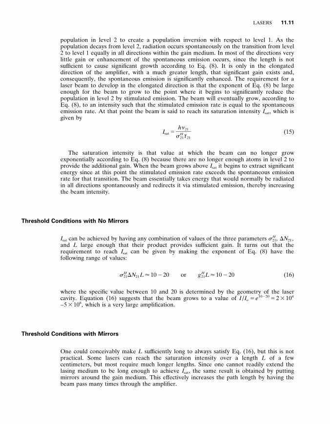
FIGURE 5 Laser-beam divergence for amplifier configurations having high gain and ( a ) no mirrors or ( b ) one mirror , and high or low gain and ( c ) two mirrors .
A simple understanding of how the mirrors af fect the beam is shown in Fig . 5 . The diagram ef fectively shows how multiple passes through the amplifier can be considered for the situation where flat mirrors are used at the ends of the amplifier . The dashed outlines that are the same size as the gain media represent the images of those gain media produced by their reflections in the mirrors . It can be seen that as the beam makes multiple passes , its divergence narrows up significantly in addition to the large increase in intensity that occurs due to amplification . For high-gain lasers , such as excimer or organic dye lasers , the beam only need pass through the amplifier a few times to reach saturation . For low-gain lasers , such as the helium-neon laser , it might take 500 passes through the amplifier in order to reach I s a t .
The laser beam that emerges from the laser is usually coupled out of the amplifier by having a partially transmitting mirror at one end of the amplifier which typically reflects most of the beam back into the medium for more growth . To ensure that the beam develops , the transmission of the output coupling mirror (as it is usually referred to) must be lower than the gain incurred by the beam during a round-trip pass through the amplifier . If the transmission is higher than the round-trip gain , the beam undergoes no net amplification . It simply never develops . Thus a relationship that describes the threshold for laser oscillation balances the laser gain with the cavity losses . In the most simplified form , those losses are due to the mirrors having a reflectivity less than unity . Thus , for a round-trip pass through the laser cavity , the threshold for inversion can be expressed as
R 1 R 2 e s 2 1 D N 2 1 2 L . 1 or R 1 R 2 e g 2 1 2 L . 1 (17 a )
which is a similar requirement to that of Eq . (16) since it defines the minimum gain requirements for a laser .
A more general version of Eq . (17 a ) can be expressed as
R 1 R 2 (1 2 a L ) 2 e ( s 2 1 D N 2 1 2 a )2 L 5 1 or R 1 R 2 (1 2 a L ) 2 e ( g 2 1 2 a )2 L 5 1 (17 b )
in which we have included a distributed absorption a throughout the length of the gain

LASERS 11 .13
medium at the laser wavelength , as well as the total scattering losses a L per pass through the cavity (excluding the gain medium and the mirror surfaces) . The absorption loss a is essentially a separate absorbing transition within the gain medium that could be a separate molecule as in an excimer laser , absorption from either the ground state or from the triplet state in a dye laser , or absorption from the ground state in the broadband tunable solid-state lasers and in semiconductor lasers or from the upper laser state in most solid-state lasers . The scattering losses a L , per pass , would include scattering at the windows of the gain medium , such as Brewster angle windows , or scattering losses from other elements that are inserted within the cavity . These are typically of the order of one or two percent or less .
Laser Operation Above Threshold
Significant power output is achieved by operating the laser at a gain greater than the threshold value defined above in Eqs . (16) and (17) . For such a situation , the higher gain that would normally be produced by increased pumping is reduced to the threshold value by stimulated emission . The additional energy obtained from the reduced population inversion is transferred to the laser beam in the form of increased laser power . If the laser has low gain , as most cw (continuously operating) gas lasers do , the gain and also the power output tend to stabilize rather readily .
For solid-state lasers , which tend to have higher gain and also a long upper-laser-level lifetime , a phenomenon known as relaxation oscillations 7 occurs in the laser output . For pulsed (non-Q-switched) lasers in which the gain lasts for many microseconds , these oscillations occur in the form of a regularly repeated spiked laser output superimposed on a lower steady-state value . For cw lasers it takes the form of a sinusoidal oscillation of the output . The phenomenon is caused by an oscillation of the gain due to the interchange of pumped energy between the upper laser level and the laser field in the cavity . This ef fect can be controlled by using an active feedback mechanism , in the form of an intensity- dependent loss , in the laser cavity .
Laser mirrors not only provide the additional length required for the laser beam to reach I s a t , but they also provide very important resonant cavity ef fects that will be discussed in a later section . Using mirrors at the ends of the laser gain medium (or amplifier) is referred to as having the gain medium located within an optical cavity .
How Population Inversions Are Achieved 4
It was mentioned earlier that population inversions are not easily achieved in normal situations . All types of matter tend to be driven towards thermal equilibrium . From an energy-level standpoint , to be in thermal equilibrium implies that the ratio of the populations of two excited states of a particular material , whether it be a gaseous , liquid , or solid material , is described by Eq . (12) . For any finite value of the temperature this leads to a value of N 2 / ( g 2 / g 1 ) N 1 that is always less than unity and therefore Eq . (14) can never be satisfied under conditions of thermal equilibrium . Population inversions are therefore produced in either one of two ways : (1) selective excitation (pumping) of the upper-laser-level 2 , or (2) more rapid decay of the population of the lower-laser-level 1 than of the upper-laser-level 2 , even if they are both populated by the same pumping process .
The first requirement mentioned above was met in producing the very first laser , the

11 .14 OPTICAL SOURCES
FIGURE 6 Energy-level diagram for a ruby laser showing the pump wavelength bands and the laser transition . The symbols 4 T 1 and 4 T 2 are shown as the appropriate designations for the pumping levels in ruby along with the more traditional designations in parenthesis .
ruby laser . 5 In this laser the flash lamp selectively pumped chromium atoms to the upper laser level (through an intermediate level) until the ground state (lower laser level) was depleted enough to produce the inversion (Fig . 6) . Another laser that uses this selective pumping process is the copper vapor laser 6 (CVL) . In this case , electrons in a gaseous discharge containing the copper vapor have a much preferred probability of pumping the upper laser level than the lower laser level (Fig . 7) . Both of these lasers involve essentially three levels .
The second type of excitation is used for most solid-state lasers , such as the Nd 3 1 doped yttrium aluminum garnet laser 7 (commonly referred to as the Nd : YAG laser) , for organic dye lasers , 8 and many others . It is probably the most common mechanism used to achieve
FIGURE 7 Energy-level diagrams of the transient three-level copper and lead vapor lasers showing the pump processes as well as the laser transitions .

LASERS 11 .15
FIGURE 8 Energy-level diagram of the Nd : YAG laser indicating the four-level laser excitation process .
the necessary population inversion . This process involves four levels 2 (although it can include more) and generally occurs via excitation from the ground state 0 to an excited state 3 which energetically lies above the upper-laser-level 2 . The population then decays from level 3 to level 2 by nonradiative processes (such as collisional processes in gases) , but can also decay radiatively to level 2 . If the proper choice of materials has been made , the lower-laser-level 1 in some systems will decay rapidly to the ground state (level 0) which allows the condition N 2 . ( g 2 / g 1 ) N 1 to be satisfied . This situation is shown in Fig . 8 for a Nd : YAG laser crystal .
Optimization of the Output Coupling from a Laser Cavity 9
A laser will operate with any combination of mirror reflectivities subject to the constraints of the threshold condition of Eq . (17 a or b ) . However , since lasers are devices that are designed to use the laser power in various applications , it is desirable to extract the most power from the laser in the most ef ficient manner . A simple expression for the optimum laser output coupling is given as
t o p t 5 ( a L g 2 1 L ) 1 / 2 2 a L (18)
in which a L is the absorption and scattering losses per pass through the amplifier (the same as in Eq . (17 a and b ) , g 2 1 is the small signal gain per pass through the amplifier , and L is the length of the gain medium . This value of t o p t is obtained by assuming that equal output couplings are used for both mirrors at the ends of the cavity . To obtain all of the power from one end of the laser , the output transmission must be doubled for one mirror and the other mirror is made to be a high reflector .
11 .16 OPTICAL SOURCES
The intensity of the beam that would be emitted from the output mirror can be estimated to be
I t m a x 5
I s a t t 2 opt
2 a L (19)
in which I s a t is the saturation intensity as obtained from Eq . (15) . If all of the power is desired from one end of the laser , as discussed above , then I t m a x
would be doubled in the above expression .
Pumping Techniques to Produce Inversions
Excitation or pumping of the upper laser level generally occurs by two techniques : (1) particle pumping and (2) optical or photon pumping . No matter which process is used , the goal is to achieve suf ficient pumping flux and , consequently enough , population in the upper-laser-level 2 to satisfy or exceed the requirements of either Eq . (16) or Eq . (17) .
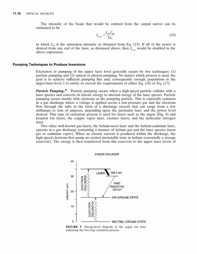
Particle Pumping . 1 0 Particle pumping occurs when a high-speed particle collides with a laser species and converts its kinetic energy to internal energy of the laser species . Particle pumping occurs mostly with electrons as the pumping particle . This is especially common in a gas discharge where a voltage is applied across a low-pressure gas and the electrons flow through the tube in the form of a discharge current that can range from a few milliamps to tens of amperes , depending upon the particular laser and the power level desired . This type of excitation process is used for lasers such as the argon (Fig . 9) and krypton ion lasers , the copper vapor laser , excimer lasers , and the molecular nitrogen laser .
Two other well-known gas lasers , the helium-neon laser and the helium-cadmium laser , operate in a gas discharge containing a mixture of helium gas and the laser species (neon gas or cadmium vapor) . When an electric current is produced within the discharge , the high-speed electrons first pump an excited metastable state in helium (essentially a storage reservoir) . The energy is then transferred from this reservoir to the upper laser levels of
FIGURE 9 Energy-level diagram of the argon ion laser indicating the two-step excitation process .

LASERS 11 .17
FIGURE 10 Energy-level diagrams of the helium-neon (He-Ne) laser and the helium-cadmium (He-Cd) laser that also include the helium metastable energy levels that transfer their energy to the upper laser levels by collisions .
neon or cadmium by collisions of the helium metastable level with the neon or cadmium ground-state atoms as shown in Fig . 10 . Electron collisions with the cadmium ion ground state have also been shown to produce excitation in the case of the helium-cadmium laser .
In an energy-transfer process similar to that of helium with neon or cadmium , the CO 2 laser operates by using electrons of the gas discharge to produce excitation of molecular nitrogen vibrational levels that subsequently transfer their energy to the vibrational upper laser levels of CO 2 as indicated in Fig . 11 . Helium is used in the CO 2 laser to control the
FIGURE 11 Energy-level diagram of the carbon dioxide (CO 2 ) laser along with the energy level of molecular nitrogen that collisionally transfers its energy to the CO 2 upper laser level .

11 .18 OPTICAL SOURCES
electron temperature and also to cool (reduce) the population of the lower laser level via collisions of helium atoms with CO 2 atoms in the lower laser level .
High-energy electron beams and even nuclear reactor particles have also been used for particle pumping of lasers , but such techniques are not normally used in commercial laser devices .
Optical Pumping . 7 Optical pumping involves the process of focusing light into the gain medium at the appropriate wavelength such that the gain medium will absorb most (or all) of the light and thereby pump that energy into the upper laser level as shown in Fig . 12 . The selectivity in pumping the laser level with an optical pumping process is determined by choosing a gain medium having significant absorption at a wavelength at which a suitable pump light source is available . This of course implies that the absorbing wavelengths provide ef ficient pumping pathways to the upper laser level . Optical pumping requires very intense pumping light sources , including flash lamps and other lasers . Lasers that are produced by optical pumping include organic dye lasers and solid-state lasers .
Flash lamps used in optically pumped laser systems are typically long , cylindrically shaped , fused quartz structures of a few millimeters to a few centimeters in diameter and 10 to 50 centimeters in length . The lamps are filled with gases such as xenon and are initiated by running an electrical current through the gas . The light is concentrated into the lasing medium by using elliptically shaped reflecting cavities that surround both the laser medium and the flash lamps as shown in Fig . 13 . These cavities ef ficiently collect and transfer to the laser rod most of the lamp energy in wavelengths within the pump absorbing band of the rod . The most common flash-lamp-pumped lasers are Nd : YAG , Nd : glass , and organic dye lasers . New crystals such as Cr : LiSAF and HoTm : YAG are also amenable to flash-lamp pumping .
Solid-state lasers also use energy-transfer processes as part of the pumping sequence in a way similar to that of the He-Ne and He-Cd gas lasers . For example , Cr 3 1 ions are added into neodymium-doped crystals to improve the absorption of the pumping light . The energy is subsequently transferred to the Nd 3 1 laser species . Such a process of adding desirable impurities is known as sensitizing .
Lasers are used as optical pumping sources in situations where (1) it is desirable to be able to concentrate the pump energy into a small-gain region or (2) it is useful to have a narrow spectral output of the pump source in contrast with the broadband spectral distribution of a flash lamp .
Laser pumping is achieved by either transverse pumping (a direction perpendicular to the direction of the laser beam) or longitudinal pumping (a direction in the same direction as the emerging laser beam) . Frequency doubled and tripled pulsed Nd : YAG lasers are
FIGURE 12 A general diagram showing optical pumping of the upper laser level .
LASERS 11 .19
FIGURE 13 Flash-lamp pumping arrangements for solid-state laser rods showing the use of helical lamps as well as linear lamps in a circular cavity , a single elliptical cavity , and a double elliptical cavity .
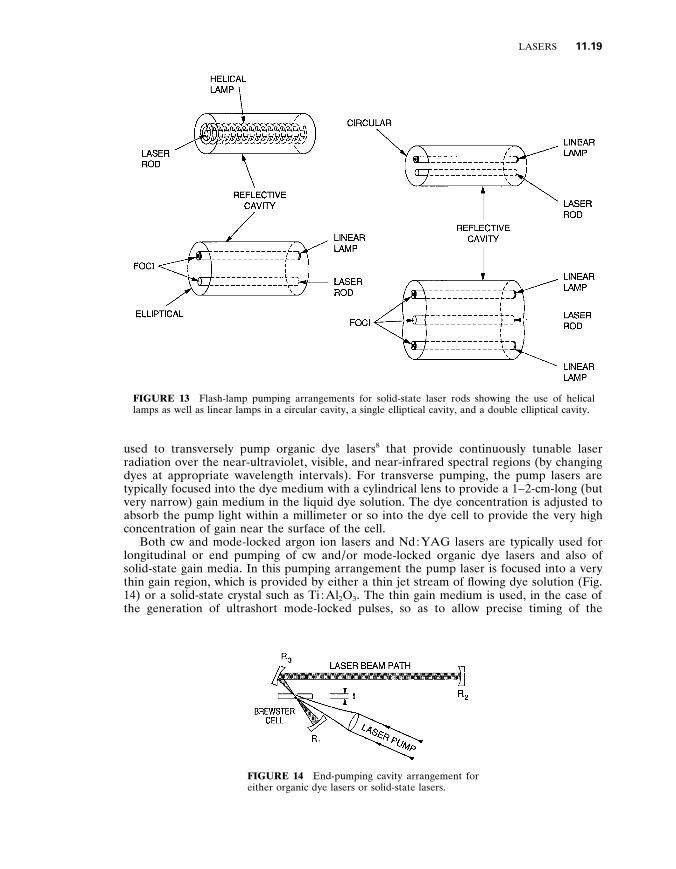
used to transversely pump organic dye lasers 8 that provide continuously tunable laser radiation over the near-ultraviolet , visible , and near-infrared spectral regions (by changing dyes at appropriate wavelength intervals) . For transverse pumping , the pump lasers are typically focused into the dye medium with a cylindrical lens to provide a 1 – 2-cm-long (but very narrow) gain medium in the liquid dye solution . The dye concentration is adjusted to absorb the pump light within a millimeter or so into the dye cell to provide the very high concentration of gain near the surface of the cell .
Both cw and mode-locked argon ion lasers and Nd : YAG lasers are typically used for longitudinal or end pumping of cw and / or mode-locked organic dye lasers and also of solid-state gain media . In this pumping arrangement the pump laser is focused into a very thin gain region , which is provided by either a thin jet stream of flowing dye solution (Fig . 14) or a solid-state crystal such as Ti : Al 2 O 3 . The thin gain medium is used , in the case of the generation of ultrashort mode-locked pulses , so as to allow precise timing of the
FIGURE 14 End-pumping cavity arrangement for either organic dye lasers or solid-state lasers .

11 .20 OPTICAL SOURCES
FIGURE 15 Pumping arrangements for diode-pumped Nd : YAG lasers showing both ( a ) standard pumping using an imaging lens and ( b ) close- coupled pumping in which the diode is located adjacent to the laser crystal .
short-duration pump pulses with the ultrashort laser pulses that develop within the gain medium as they travel within the optical cavity .
Gallium arsenide semiconductor diode lasers , operating at wavelengths around 0 . 8 m m , can be ef fectively used to pump Nd : YAG lasers because the laser wavelength is near that of the strongest absorption feature of the pump band of the Nd : YAG laser crystal , thereby minimizing excess heating of the laser medium . Also , the diode lasers are very ef ficient light sources that can be precisely focused into the desired mode volume of a small Nd : YAG crystal (Fig . 15 a ) which results in minimal waste of the pump light . Figure 15 b shows how close-coupling of the pump laser and the Nd : YAG crystal can be used to provide compact ef ficient diode laser pumping . The infrared output of the Nd : YAG laser can then also be frequency doubled as indicated in Fig . 15 a , using nonlinear optical techniques to produce a green laser beam in a relatively compact package .
1 1 . 4 LASER PROPERTIES ASSOCIATED WITH OPTICAL CAVITIES OR RESONATORS
Longitudinal Laser Modes 1 , 2
When a collimated optical beam of infinite lateral extent (a plane wave) passes through two reflecting surfaces of reflectivity R and also of infinite extent that are placed normal (or nearly normal) to the beam and separated by a distance d , as shown in Fig . 16 a , the
LASERS 11 .21
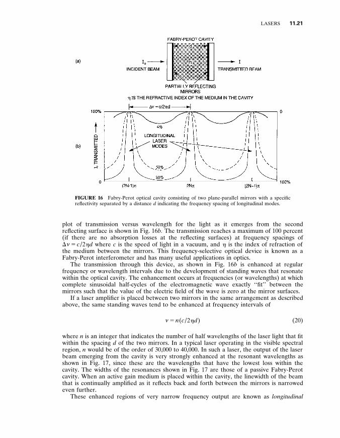
FIGURE 16 Fabry-Perot optical cavity consisting of two plane-parallel mirrors with a specific reflectivity separated by a distance d indicating the frequency spacing of longitudinal modes .
plot of transmission versus wavelength for the light as it emerges from the second reflecting surface is shown in Fig . 16 b . The transmission reaches a maximum of 100 percent (if there are no absorption losses at the reflecting surfaces) at frequency spacings of D … 5 c / 2 h d where c is the speed of light in a vacuum , and h is the index of refraction of the medium between the mirrors . This frequency-selective optical device is known as a Fabry-Perot interferometer and has many useful applications in optics .
The transmission through this device , as shown in Fig . 16 b is enhanced at regular frequency or wavelength intervals due to the development of standing waves that resonate within the optical cavity . The enhancement occurs at frequencies (or wavelengths) at which complete sinusoidal half-cycles of the electromagnetic wave exactly ‘‘fit’’ between the mirrors such that the value of the electric field of the wave is zero at the mirror surfaces .
If a laser amplifier is placed between two mirrors in the same arrangement as described above , the same standing waves tend to be enhanced at frequency intervals of
… 5 n ( c / 2 h d ) (20)
where n is an integer that indicates the number of half wavelengths of the laser light that fit within the spacing d of the two mirrors . In a typical laser operating in the visible spectral region , n would be of the order of 30 , 000 to 40 , 000 . In such a laser , the output of the laser beam emerging from the cavity is very strongly enhanced at the resonant wavelengths as shown in Fig . 17 , since these are the wavelengths that have the lowest loss within the cavity . The widths of the resonances shown in Fig . 17 are those of a passive Fabry-Perot cavity . When an active gain medium is placed within the cavity , the linewidth of the beam that is continually amplified as it reflects back and forth between the mirrors is narrowed even further .
These enhanced regions of very narrow frequency output are known as longitudinal
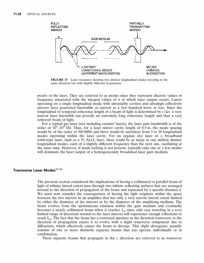
11 .22 OPTICAL SOURCES
FIGURE 17 Laser resonator showing two distinct longitudinal modes traveling in the same direction but with slightly dif ferent frequencies .
modes of the laser . They are referred to as modes since they represent discrete values of frequency associated with the integral values of n at which laser output occurs . Lasers operating on a single longitudinal mode with ultrastable cavities and ultrahigh reflectivity mirrors have generated linewidths as narrow as a few hundred hertz or less . Since the longitudinal or temporal coherence length of a beam of light is determined by c / D … , a very narrow laser linewidth can provide an extremely long coherence length and thus a very coherent beam of light .
For a typical gas laser (not including excimer lasers) , the laser gain bandwidth is of the order of 10 9 – 10 1 0 Hz . Thus , for a laser mirror cavity length of 0 . 5 m , the mode spacing would be of the order of 300 MHz and there would be anywhere from 3 to 30 longitudinal modes operating within the laser cavity . For an organic dye laser or a broadband solid-state laser , such as a Ti : Al 2 O 3 laser , there could be as many as one million distinct longitudinal modes , each of a slightly dif ferent frequency than the next one , oscillating at the same time . However , if mode-locking is not present , typically only one or a few modes will dominate the laser output of a homogeneously broadened laser gain medium .
Transverse Laser Modes 11–14
The previous section considered the implications of having a collimated or parallel beam of light of infinite lateral extent pass through two infinite reflecting surfaces that are arranged normal to the direction of propagation of the beam and separated by a specific distance d . We must now consider the consequences of having the light originate within the space between the two mirrors in an amplifier that has only a very narrow lateral extent limited by either the diameter of the mirrors or by the diameter of the amplifying medium . The beam evolves from the spontaneous emission within the gain medium and eventually becomes a nearly collimated beam when it reaches I s a t since only rays traveling in a very limited range of directions normal to the laser mirrors will experience enough reflections to reach I s a t . The fact that the beam has a restricted aperture in the direction transverse to the direction of propagation causes it to evolve with a slight transverse component due to dif fraction , which ef fectively causes the beam to diverge . This slight divergence actually consists of one or more distinctly separate beams that can operate individually or in combination .
These separate beams that propagate in the z direction are referred to as trans y erse

LASERS 11 .23
FIGURE 18 Laser resonator showing two distinct transverse modes traveling in dif ferent directions with slightly dif ferent frequencies .
modes as shown in Fig . 18 . They are characterized by the various lateral spatial distributions of the electric field vector E ( x , y ) in the x - y directions as they emerge from the laser . These transverse amplitude distributions for the waves can be described by the relationship .
E p q ( x , y ) 5 H p S 4 2 x
w D H q S 4 2 y
w D e 2 ( x 2 1 y 2 )/ w 2
(21)
In this solution , p and q are positive integers ranging from zero to infinity that designate the dif ferent modes which are associated with the order of the Hermite polynomials . Thus every set of p , q represents a specific distribution of wave amplitude at one of the mirrors , or a specific transverse mode of the open-walled cavity . We can list several Hermite polynomials as follows :
H 0 ( u ) 5 1 H 1 ( u ) 5 2 u
H 2 ( u ) 5 2(2 u 2 2 1) (22)
H m ( u ) 5 ( 2 1) m e u 2 d m ( e 2 u 2 )
du m
The spatial intensity distribution would be obtained by squaring the amplitude distribution function of Eq . (21) . The transverse modes are designated TEM for transverse electro- magnetic . The lowest-order mode is given by TEM 0 0 . It could also be written as TEM n 00 in which n would designate the longitudinal mode number [Equation (20)] . Since this number is generally very large for optical frequencies , it is not normally given .
The lowest order TEM 0 0 mode , has a circular distribution with a gaussian shape (often referred to as the gaussian mode ) and has the smallest divergence of any of the transverse modes . Such a mode can be focused to a spot size with dimensions of the order of the wavelength of the beam . It has a minimum width or waist 2 w o that is typically located between the laser mirrors (determined by the mirror curvatures and separation) and expands symmetrically in opposite directions from that minimum waist according to the following equation :
w ( z ) 5 w o F 1 1 S l z h π w 2
o D 2 G 1/2
5 w o F 1 1 S z z o D 2 G 1/2
(23)
where w ( z ) is the beam waist at any location z measured from w o , h is the index of

11 .24 OPTICAL SOURCES
FIGURE 19 Parameters of a gaussian-shaped beam which are the features of a TEM 0 0 transverse laser mode .
refraction of the medium , and z o 5 h π w 2 o / l is the distance over which the beam waist
expands to a value of 4 2 w o . The waist w ( z ) at any location , as shown in Fig . 19 , describes the transverse dimension
within which the electric field distribution of the beam decreases to a value of 37 percent (1 / e ) of its maximum on the beam axis and within which 86 . 5 percent of the beam energy is contained . The TEM 0 0 mode would have an intensity distribution that is proportional to the square of Eq . (21) for p 5 q 5 0 and , since it is symmetrical around the axis of propagation , it would have a cylindrically symmetric distribution of the form
I ( r , z ) 5 I o e 2 2 r 2 / w 2 ( z ) (24)
where I o is the intensity on the beam axis . The beam also has a wavefront curvature given by
R ( z ) 5 z F 1 1 S h π w 2 o
l z D 2 G (25)
which is indicated in Fig . 19 , and a far-field angular divergence given by
θ 5 lim z 5 ̀
2 w ( z ) z
5 2 l
π w o 5 0 . 64
l
w o (26)
For a symmetrical cavity formed by two mirrors , each of radius of curvature R , separated by a distance d and in a medium in which h 5 1 the minimum beam waist w o is given by
w 2 o 5
l
2 π [ d (2 R 2 d )] 1 / 2 (27)
and the radius of curvature r c of the wavefront is
r c 5 z 1 d (2 R 2 d )
4 z (28)

LASERS 11 .25
FIGURE 20 A stable laser resonator indicating the beam profile at various locations along the beam axis as well as the wavefront at the mirrors that matches the curvature of the mirrors .
For a confocal resonator in which R 5 d , w o is given by
w o 5 – l d 2 π
(29)
and the beam waist (spot size) at each mirror located a distance d / 2 from the minimum is
w 5 – l d π
(30)
Thus , for a confocal resonator , w ( d / 2) at each of the mirrors is equal to 4 2 w o and thus at that location , z 5 z o . The distance between mirrors for such a cavity configuration is referred to as the confocal parameter b such that b 5 2 z o . In a stable resonator , the curvature of the wavefront at the mirrors , according to Eqs . (25) and (28) , exactly matches the curvature of the mirrors as shown in Fig . 20 .
Each individual transverse mode of the beam is produced by traveling a specific path between the laser mirrors such that , as it passes from one mirror to the other and returns , the gain it receives from the amplifier is at least as great as the total losses of the mirror , as indicated from Eq . (17) , plus the additional dif fraction losses produced by either the finite lateral extent of the laser mirrors or the finite diameter of the laser amplifier or some other optical aperture placed in the system , whichever is smaller . Thus the TEM 0 0 mode is produced by a beam passing straight down the axis of the resonator as indicated in Fig . 19 .
Laser Resonator Configurations and Cavity Stability 4 ,14
There are a variety of resonator configurations that can be used for lasers . The use of slightly curved mirrors leads to much lower dif fraction losses of the transverse modes than do plane parallel mirrors , and they also have much less stringent alignment tolerances . Therefore , most lasers use curved mirrors for the optical cavity . For a cavity with two
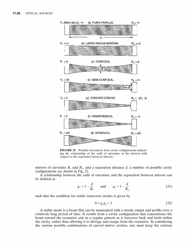
11 .26 OPTICAL SOURCES
FIGURE 21 Possible two-mirror laser cavity configurations indicat- ing the relationship of the radii of curvature of the mirrors with respect to the separation between mirrors .
mirrors of curvature R 1 and R 2 , and a separation distance d , a number of possible cavity configurations are shown in Fig . 21 .
A relationship between the radii of curvature and the separation between mirrors can be defined as
g 1 5 1 2 d
R 1 and g 2 5 1 2
d R 2
(31)
such that the condition for stable transverse modes is given by
0 , g 1 g 2 , 1 (32)
A stable mode is a beam that can be maintained with a steady output and profile over a relatively long period of time . It results from a cavity configuration that concentrates the beam toward the resonator axis in a regular pattern as it traverses back and forth within the cavity , rather than allowing it to diverge and escape from the resonator . In considering the various possible combinations of curved mirror cavities , one must keep the relation

LASERS 11 .27
FIGURE 22 Stability diagram for two-mirror laser cavities indicating the shaded regions where stable cavities exist .
between the curvatures and mirror separation d within the stable regions of the graph , as shown in Fig . 22 , in order to produce stable modes . Thus it can be seen from Fig . 22 that not all configurations shown in Fig . 21 are stable . For example , the planar , confocal , and concentric arrangements are just on the edge of stability according to Fig . 22 .
There may be several transverse modes oscillating simultaneously ‘‘within’’ a single longitudinal mode . Each transverse mode can have the same value of n [Eq . (20)] but will have a slightly dif ferent value of d as it travels a dif ferent optical path between the resonator mirrors , thereby generating a slight frequency shift from that of an adjacent transverse mode . For most optical cavities , the mode that operates most easily is the TEM 0 0 mode , since it travels a direct path along the axis of the gain medium .
1 1 . 5 SPECIAL LASER CAVITIES
Unstable Resonators 1 4
A laser that is operating in a TEM 0 0 mode , as outlined above , typically has a beam within the laser cavity that is relatively narrow in width compared to the cavity length . Thus , if a laser with a relatively wide gain region is used , to obtain more energy in the output beam , it is not possible to extract the energy from that entire region from a typically very narrow low-order gaussian mode . A class of resonators has been developed that can extract the energy from such wide laser volumes and also produce a beam with a nearly gaussian

11 .28 OPTICAL SOURCES
FIGURE 23 Unstable resonator cavity configurations show- ing both the negative and positive branch confocal cavities .
profile that makes it easily focusable . These resonators do not meet the criteria for stability , as outlined above , but still provide a good beam quality for some types of lasers . This class of resonators is referred to as unstable resonators .
Unstable resonators are typically used with high-gain laser media under conditions such that only a few passes through the amplifier will allow the beam to reach the saturation intensity and thus extract useful energy . A diagram of two unstable resonator cavity configurations is shown in Fig . 23 . Figure 23 b is the positive branch confocal geometry and is one of the most common unstable resonator configurations . In this arrangement , the small mirror has a convex shape and the large mirror a concave shape with a separation of length d such that R 2 2 R 1 5 2 d . With this configuration , any ray traveling parallel to the axis from left to right that intercepts the small convex mirror will diverge toward the large convex mirror as though it came from the focus of that mirror . The beam then reflects of f of the larger mirror and continues to the right as a beam parallel to the axis . It emerges as a reasonably well-collimated beam with a hole in the center (due to the obscuration of the small mirror) . The beam is designed to reach the saturation intensity when it arrives at the large mirror and will therefore proceed to extract energy as it makes its final pass through the amplifier . In the far field , the beam is near gaussian in shape , which allows it to be propagated and focused according to the equations described in the previous section . A number of dif ferent unstable resonator configurations can be found in the literature for specialized applications .
Q-Switching 1 5
A typical laser , after the pumping or excitation is first applied , will reach the saturation intensity in a time period ranging from approximately 10 nsec to 1 m sec , depending upon the value of the gain in the medium . For lasers such as solid-state lasers the upper-laser-level lifetime is considerably longer than this time (typically 50 – 200 m sec) . It

LASERS 11 .29
is possible to store and accumulate energy in the form of population in the upper laser level for a time duration of the order of that upper-level lifetime . If the laser cavity could be obscured during this pumping time and then suddenly switched into the system at a time order of the upper-laser-level lifetime , it would be possible for the gain , as well as the laser energy , to reach a much larger value than it normally would under steady-state conditions . This would produce a ‘‘giant’’ laser pulse of energy from the system .
Such a technique can in fact be realized and is referred to as Q - switching to suggest that the cavity Q is changed or switched into place . The cavity is switched on by using either a rapidly rotating mirror or an electro-optic shutter such as a Pockel cell or a Kerr cell . Nd : YAG and Nd : glass lasers are the most common Q-switched lasers . A diagram of the sequence of events involved in Q-switching is shown in Fig . 24 .
Another technique that is similar to Q-switching is referred to as ca y ity dumping . With this technique , the intense laser beam inside of a normal laser cavity is rapidly switched out of the cavity by a device such as an acousto-optic modulator . Such a device is inserted at Brewster’s angle inside the cavity and is normally transparent to the laser beam . When the device is activated , it rapidly inserts a high-reflecting surface into the cavity and reflects the beam out of the cavity . Since the beam can be as much as two orders of magnitude higher in intensity within the cavity than that which leaks through an output mirror , it is possible to extract high power on a pulsed basis with such a technique .
Mode-Locking 1 4
In the discussion of longitudinal modes it was indicated that such modes of intense laser output occur at regularly spaced frequency intervals of D … 5 c / 2 h d over the gain bandwidth of the laser medium . For laser cavity lengths of the order of 10 – 100 cm these frequency intervals range from approximately 10 8 to 10 9 Hz . Under normal laser operation , specific modes with the highest gain tend to dominate and quench other modes (especially if the gain medium is homogeneously broadened) . However , under certain conditions it is possible to obtain all of the longitudinal modes lasing simultaneously , as shown in Fig . 25 a . If this occurs , and the modes are all phased together so that they can act in concert by constructively and destructively interfering with each other , it is possible to produce a series of giant pulses separated in a time D t of
D t 5 2 h d / c (33)
or approximately 1 – 10 nsec for the cavity lengths mentioned above (see Fig . 25 b ) . The pulse duration is approximately the reciprocal of the separation between the two extreme longitudinal laser modes or
D t p 5 1
n D … (34)
as can also be seen in Fig . 25 b . This pulse duration is approximately the reciprocal of the laser gain bandwidth . However , if the index of refraction varies significantly over the gain bandwidth , then all of the frequencies are not equally spaced and the mode-locked pulse duration will occur only within the frequency width over which the frequency separations are approximately the same .
The narrowest pulses are produced from lasers having the largest gain bandwidth such as organic dye lasers , and solid-state lasers including Ti : Al 2 O 3 , Cr : Al 2 O 3 , and Cr : LiSAlF . The shortest pulses to date , of the order of 6 3 10 2 1 5 sec , are produced in

11 .30 OPTICAL SOURCES
FIGURE 24 Schematic diagram of a Q-switched laser indicating how the loss is switched out of the cavity and a gaint laser pulse is produced as the gain builds up .
organic dyes where the gain bandwidth is approximately 50 nm at a center wavelength of 600 nm .
Such short-pulse operation is referred to as mode - locking and is achieved by inserting a very fast shutter within the cavity which is opened and closed at the intervals of the round-trip time of the short laser pulse within the cavity . This shutter coordinates the time at which all of the modes arrive at the mirror and thus brings them all into phase at that location . Electro-optic shutters , short duration gain pumping by another mode-locked laser , or passive saturable absorbers are techniques that can serve as the fast shutter . The second technique , short-duration gain pumping , is referred to as synchronous pumping . Three fast saturable absorber shutter techniques for solid-state lasers include colliding pulse mode-locking , 1 6 additive pulse mode-locking , 1 7 and Kerr lens mode-locking . 1 8
Distributed Feedback Lasers 1 9
The typical method of obtaining feedback into the laser gain medium is to have the mirrors located at the ends of the amplifier as discussed previously . It is also possible , however , to provide the reflectivity within the amplifying medium in the form of a periodic variation of either the gain or the index of refraction throughout the medium . This process is referred to as distributed feedback or DFB . Such feedback methods are particularly ef fective in

LASERS 11 .31
FIGURE 25 Diagrams in both the frequency and time domains of how mode-locking is produced by phasing n longitudinal modes together to produce an ultrashort laser pulse .
semiconductor lasers in which the gain is high and the fabrication of periodic variations is not dif ficult . The reader is referred to the reference section at the end of this chapter for further information concerning this type of feedback .
Ring Lasers 1 4
Ring lasers are lasers that have an optical path within the cavity that involves the beam circulating in a loop rather than passing back and forth over the same path . This requires optical cavities that have more than two mirrors . The laser beam within the cavity consists of two waves traveling in opposite directions with separate and independent resonances within the cavity . In some instances an optical device is placed within the cavity that provides a unidirectional loss . This loss suppresses one of the beams , allowing the beam propagating in the other direction to become dominant . The laser output then consists of a traveling wave instead of a standing wave and therefore there are no longitudinal modes . Such an arrangement also eliminates the variation of the gain due to the standing waves in the cavity (spatial hole burning) , and thus the beam tends to be more homogeneous than

11 .32 OPTICAL SOURCES
that of a normal standing-wave cavity . Ring lasers are useful for producing ultrashort mode-locked pulses and also for use in laser gyroscopes as stable reference sources .
1 1 . 6 SPECIFIC TYPES OF LASERS
Lasers can be categorized in several dif ferent ways including wavelength , material type , and applications . In this section we will summarize them by material type such as gas , liquid , solid-state , and semiconductor lasers . We will include only lasers that are available commercially since such lasers now provide a very wide range of available wavelengths and powers without having to consider special laboratory lasers .
Gaseous Laser Gain Media
Helium - Neon Laser . 1 0 The helium-neon laser was the first gas laser . The most widely used laser output wavelength is a red beam at 632 . 8 nm with a cw output ranging from 1 to 100 mW and sizes ranging from 10 to 100 cm in length . It can also be operated at a wavelength of 543 . 5 nm for some specialized applications . The gain medium is produced by passing a relatively low electrical current (10 mA) through a low pressure gaseous discharge tube containing a mixture of helium and neon . In this mixture , helium metastable atoms are first excited by electron collisions as shown in Fig . 10 . The energy is then collisionally transferred to neon atom excited states which serve as upper laser levels .
Argon Ion Laser . 1 0 The argon ion laser and the similar krypton ion laser operate over a wide range of wavelengths in the visible and near-ultraviolet regions of the spectrum . The wavelengths in argon that have the highest power are at 488 . 0 and 514 . 5 nm . Power outputs on these laser transitions are available up to 20 W cw in sizes ranging from 50 – 200 cm in length . The gain medium is produced by running a high electric current (many amperes) through a very low pressure argon or krypton gas . The argon atoms must be ionized to the second and third ionization stages (Fig . 9) in order to produce the population inversions . As a result , these lasers are inherently inef ficient devices .
Helium - Cadmium Laser . 1 0 The helium-cadmium laser operates cw in the blue at 441 . 6 nm , and in the ultraviolet at 353 . 6 and 325 . 0 nm with powers ranging from 20 – 200 mW in lasers ranging from 40 – 100 cm in length . The gain medium is produced by heating cadmium metal and evaporating it into a gaseous discharge of helium where the laser gain is produced . The excitation mechanisms include Penning ionization (helium metastables collide with cadmium atoms) and electron collisional ionization within the discharge as indicated in Fig . 10 . The laser uses an ef fect known as cataphoresis to transport the cadmium through the discharge and provide the uniform gain medium .
Copper Vapor Laser . 1 0 This pulsed laser provides high-average powers of up to 100 W at wavelengths of 510 . 5 and 578 . 2 nm . The copper laser and other metal vapor lasers of this class , including gold and lead lasers , typically operate at a repetition rate of up to 20 kHz with a current pulse duration of 10 – 50 nsec and a laser output of 1 – 10 mJ / pulse . The copper lasers operate at temperatures in the range of 1600 8 C in 2 – 10-cm-diameter temperature-resistant tubes typically 100 – 150 cm in length . The lasers are self-heated such

LASERS 11 .33
that all of the energy losses from the discharge current provide heat to bring the plasma tube to the required operating temperature . Excitation occurs by electron collisions with copper atoms vaporized in the plasma tube as indicated in Fig . 7 .
Carbon - Dioxide Laser . 1 0 The CO 2 laser , operating primarily at a wavelength of 10 . 6 m m , is one of the most powerful lasers in the world , producing cw powers of over 100 kW and pulsed energies of up to 10 kJ . It is also available in small versions with powers of up to 100 W from a laser the size of a shoe box . CO 2 lasers typically operate in a mixture of carbon dioxide , nitrogen , and helium gases . Electron collisions excite the metastable levels in nitrogen molecules with subsequent transfer of that energy to carbon dioxide laser levels as shown in Fig . 11 . The helium gas acts to keep the average electron energy high in the gas discharge region and to cool or depopulate the lower laser level . This laser is one of the most ef ficient lasers , with conversion from electrical energy to laser energy of up to 30 percent .
Excimer Laser . 2 0 The rare gas-halide excimer lasers operate with a pulsed output primarily in the ultraviolet spectral region at 351 nm in xenon fluoride , 308 nm in xenon chloride , 248 nm in krypton fluoride , and 193 nm in argon fluoride . The laser output , with pulse durations of 10 – 50 nsec , is typically of the order of 0 . 2 – 1 . 0 J / pulse at repetition rates up to several hundred Hz . The lasers are relatively ef ficient (1 to 5 percent) and are of a size that would fit on a desktop . The excitation occurs via electrons within the discharge colliding with and ionizing the rare gas molecules and at the same time disassociating the halogen molecules to form negative halogen ions . These two species then combine to form an excited molecular state of the rare gas-halogen molecule which serves as the upper laser state . The molecule then radiates at the laser transition and the lower level advantageously disassociates since it is unstable , as shown in Fig . 26 , for the ArF excimer molecule . The excited laser state is an excited state dimer which is referred to as an excimer state .
X - Ray Laser . 2 4 Laser output in the soft-x-ray spectral region has been produced in plasmas of highly ionized ions of a number of atomic species . The highly ionized ions are
FIGURE 26 Energy-level diagram of an argon fluoride (ArF) excimer laser showing the stable excited state (upper laser level) and the unstable or repulsive ground state .
11 .34 OPTICAL SOURCES
produced by the absorption of powerful solid-state lasers focused onto solid material of the desired atomic species . Since mirrors are not available for most of the soft-x-ray laser wavelengths (4 – 30 nm) , the gain has to be high enough to obtain laser output in a single pass through the laser amplifier [Eq . (16)] . The lasers with the highest gain are the selenium laser (Se 2 4 1 ) at 20 . 6 and 20 . 9 nm and the germanium laser (Ge 2 2 1 ) at 23 . 2 , 23 . 6 , and 28 . 6 nm .
Liquid Laser Gain Media
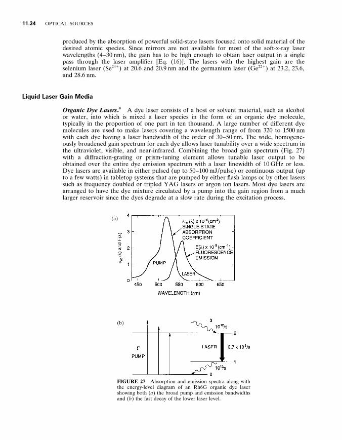
Organic Dye Lasers . 8 A dye laser consists of a host or solvent material , such as alcohol or water , into which is mixed a laser species in the form of an organic dye molecule , typically in the proportion of one part in ten thousand . A large number of dif ferent dye molecules are used to make lasers covering a wavelength range of from 320 to 1500 nm with each dye having a laser bandwidth of the order of 30 – 50 nm . The wide , homogene- ously broadened gain spectrum for each dye allows laser tunability over a wide spectrum in the ultraviolet , visible , and near-infrared . Combining the broad gain spectrum (Fig . 27) with a dif fraction-grating or prism-tuning element allows tunable laser output to be obtained over the entire dye emission spectrum with a laser linewidth of 10 GHz or less . Dye lasers are available in either pulsed (up to 50 – 100 mJ / pulse) or continuous output (up to a few watts) in tabletop systems that are pumped by either flash lamps or by other lasers such as frequency doubled or tripled YAG lasers or argon ion lasers . Most dye lasers are arranged to have the dye mixture circulated by a pump into the gain region from a much larger reservoir since the dyes degrade at a slow rate during the excitation process .
(a)
(b)
FIGURE 27 Absorption and emission spectra along with the energy-level diagram of an Rh6G organic dye laser showing both ( a ) the broad pump and emission bandwidths and ( b ) the fast decay of the lower laser level .

LASERS 11 .35
Dye lasers , with their broad gain spectrum , are particularly attractive for producing ultrashort mode-locked pulses . The shortest light pulses ever generated , of the order of 6 3 10 2 1 5 sec , were produced with mode-locked dye lasers . A mode-locked dye laser cavity is shown in Fig . 14 with a thin dye gain region located within an astigmatically compensated laser cavity .
Dielectric Solid-State Laser Gain Media
Ruby Laser . 5 , 7 The ruby laser , with an output at 694 . 3 nm , was the first laser ever developed . It consisted of a sapphire (Al 2 O 3 ) host material into which was implanted a chromium laser species in the form of Cr 3 1 ions at a concentration of 0 . 05 percent as the amplifying medium . The ruby laser involves a three-level optical pumping scheme , with the excitation provided by flash lamps , and operates either in a pulsed or cw mode . The three-level scheme for the ruby laser (Fig . 6) requires a large fraction of the population to be pumped out of the ground state before an inversion occurs . Therefore , the ruby laser is not as ef ficient as other solid-state lasers such as the Nd : YAG laser which employs a four-level pumping scheme (Fig . 8) . It is therefore no longer used as much as it was in the early days .
Nd : YAG and Nd : Glass Lasers . 7 Neodymium atoms , in the form of Nd 3 1 ions , are doped into host materials , including crystals such as yttrium-aluminum-garnet (YAG) and various forms of glass , in concentrations of approximately one part per hundred . The pumping scheme is a four-level system as shown in Fig . 8 . When implanted in YAG crystals to produce what is referred to as an Nd : YAG laser , the laser emits primarily at 1 . 06 m m with continuous powers of up to 250 W and with pulsed powers as high as several MW . Dif ficulties in growing Nd : YAG crystals limit the size of commonly used laser rods to a maximum of 1 cm in diameter and 10 cm in length . Although this size limitation is somewhat restrictive , a YAG crystal has the advantage of high thermal conductivity allowing the rapid removal of wasted heat due to inef ficient excitation . Slab geometries have recently been developed to compensate for focusing due to thermal gradients and gradient-induced stresses within the amplifier medium , thereby allowing higher average powers to be achieved . Ef ficient GaAs laser diodes are also being used to pump Nd : YAG amplifiers (see Fig . 15) since the diode pump wavelength matches a very strong pump absorption wavelength for the Nd 3 1 ion . This absorption wavelength is near the threshold pump energy , thereby minimizing the generation of wasted heat . Also , the diode pump laser can be made to more ef ficiently match the Nd laser mode volume than can a flash lamp .
Under long-pulse , flash-lamp-pumped operation , Nd : YAG lasers can produce 5 J / pulse at 100 Hz from a single rod . The pulses are trains of relaxation oscillation spikes lasting 3 – 4 msec which is obtained by powerful , long-pulse flash-lamp pumping . Q-switched Nd : YAG lasers , using a single Nd : YAG laser rod , can provide pulse energies of up to 1 . 5 J / pulse at repetition rates up to 50 Hz (75 W of average power) .
Nd : glass lasers have several advantages over Nd : YAG lasers . They can be made in much larger sizes , allowing the construction of very large amplifiers . Nd : glass has a wider gain bandwidth which makes possible the production of shorter mode-locked pulses and a lower stimulated emission cross section . The latter property allows a larger population inversion to be created and thus more energy to be stored before energy is extracted from the laser . Nd : glass amplifiers operate at a wavelength near that of Nd : YAG , at 1 . 054 m m , for example , with phosphate glass , with a gain bandwidth 10 – 15 times broader than that of Nd : YAG . This larger gain bandwidth lowers the stimulated emission cross section compared to that of Nd : YAG , which allows increased energy storage when used as an amplifier , as mentioned above .

11 .36 OPTICAL SOURCES
FIGURE 28 Absorption and emission spectra of a Ti : Al 2 O 3 laser crystal showing the extremely broad emission (gain) spectrum for this material .
The large Nd : glass lasers system at Lawrence Livermore National Laboratory , referred to as NOVA , has produced a pulse energy of 100 KJ at the fundamental frequency and 40 KJ at the third harmonic frequency at 351 nm . This system was developed for studies associated with the inertial confinement laser fusion program .
Ti : Al 2 O 3 Laser and Other Broad Bandwidth Solid-State Lasers . 7
Another class of solid-state lasers provides emission and gain over a bandwidth of the order of 100 – 400 nm in the near-infrared , as indicated in Fig . 28 . The pump absorption band is in the visible spectrum , thus allowing such pump sources as flash lamps and other lasers . The Ti : AL 2 O 3 laser is perhaps the most well-known laser of this category in that it has the widest bandwidth , covering a wavelength range from 0 . 67 m m to greater than 1 . 07 m m . Other lasers of this type include alexandrite (Cr : BeAl 2 O 4 ) , lasing from 0 . 7 to 0 . 8 m m , and Cr : LiSAF which lases from 0 . 8 to 1 . 05 m m . These lasers are used in applications where either wide tunability or short-pulse production are desired . Pulses as short as 40 fsec have been produced with mode-locked versions of these lasers . Ti : Al 2 O 3 lasers , although of fering very wide gain bandwidth , have relatively short upper-laser-level lifetimes (3 m sec) , thereby making them less ef ficient when pumping with conventional flash lamps . Cr : LiSAF lasers have longer upper-level lifetimes (67 m sec) , closer to that of Nd : YAG or Nd : glass and have demonstrated ef ficient laser operation with pumping technologies developed for Nd : YAG lasers .
Color - Center Laser . 2 1 Color-center laser gain media are produced by a dif ferent form of impurity species than most solid-state lasers . Special defect centers (F-centers) are produced within alkali-halide crystals at a density of 1 part in 10 , 000 by irradiation with x rays . These defect centers have absorbing regions in the visible portion of the spectrum and emission (and gain) in the near-infrared . A variety of crystals are used to span the laser wavelength spectrum from 0 . 8 to 4 . 0 m m . Disadvantages of color-center lasers

LASERS 11 .37
include operation at temperatures well below room temperature and the necessity to re-form the color centers at intervals of weeks or months in most cases .
Semiconductor Laser Gain Media
Semiconductor Lasers . 2 2 Semiconductor or diode lasers , typically about the size of a grain of salt , are the smallest lasers yet devised . They consist of a p - n junction formed in semiconductor crystal such as GaAs or InP in which the p -type material has an excess of holes (vacancies due to missing electrons) and the n -type material has an excess of electrons . When these two types of materials are brought together to form a junction , and an electric field in the form of a voltage is applied across the junction in the appropriate direction , the electrons and holes are brought together and recombine to produce recombination radiation at or near the wavelength associated with the bandgap energy of the material . The population of electrons and holes within the junction provides the upper-laser-level population , and the recombination radiation spectrum is the gain bandwidth D … of the laser , typically of the order of 0 . 5 to 1 . 0 nm .
The extended gain length required for these lasers is generally provided by partially reflecting cleaved parallel faces at the ends of the crystals which serve as an optical cavity . Because the cavity is so short , the longitudinal modes are spaced far apart in frequency ( D … > 1 – 5 3 10 1 1 Hz or several tenths of a nanometer) , and thus it is possible to obtain single longitudinal mode operation in such lasers . They require a few volts to operate with milliamperes of current .
Heterostructure semiconductor lasers include additional layers of dif ferent materials of similar electronic configurations , such as aluminum , indium , and phosphorous , grown adjacent to the junction to help confine the electron current to the junction region in order to minimize current and heat dissipation requirements (see Fig . 29) . The laser mode in the transverse direction is either controlled by gain guiding , in which the gain is produced over a specific narrow lateral extent determined by fabrication techniques , or by index guiding , in which the index of refraction in the transverse direction is varied to provide total internal reflection of a guided mode . Quantum-well lasers have a smaller gain region (cross section) , which confines the excitation current and thus the laser mode to an even smaller lateral region , thereby significantly reducing the threshold current and also the heat
FIGURE 29 A typical heterostructure semiconductor laser showing the various layers of dif ferential materials and the narrow region where current flows to produce the gain region in the active layer .

11 .38 OPTICAL SOURCES
dissipation requirements . Because of these low threshold requirements , quantum-well semiconductor lasers are used almost exclusively for most semiconductor laser applications .
Multiple semiconductor lasers fabricated within the same bulk structure , known as semiconductor arrays , can be operated simultaneously to produce combined cw power outputs of up to 10 W from a laser crystal of dimensions of the order of 1 mm or less . Semiconductor lasers have also been fabricated in multiple arrays mounted vertically on a chip with the mirrors in the plane of the chip . They are known as y ertical ca y ity semiconductor lasers . Each of the individual lasers has dimensions of the order of 5 m m and can be separately accessed and excited .
Semiconductor lasers operate over wavelengths ranging from 0 . 63 to 1 . 65 m m by using special doping materials to provide the expanded or contracted bandgap energies that provide the varied wavelengths . Also , new semiconductor lasers in the blue-green spectral region in crystals of ZnSe have recently been developed , but presently operate only at temperatures well below room temperature .
Laser Gain Media in Vacuum
Free Electron Laser . 2 3 Free-electron lasers are significantly dif ferent than any other type of laser in that the laser output does not result from transitions between discrete energy levels in specific materials . Instead , a high-energy beam of electrons , such as that produced by a synchrotron , traveling in a vacuum with kinetic energies of the order of 1 MeV , are directed to pass through a spatially varying magnetic field produced by two regular arrays of alternating magnet poles located on opposite sides of the beam as shown in Fig . 30 . The alternating magnetic field causes the electrons to oscillate back and forth in a direction transverse to the beam direction . The frequency of oscillation is determined by the electron beam energy , the longitudinal spacing of the alternating poles (the magnet period) , and the separation between the magnet arrays on opposite sides of the beam . The transverse oscillation of the electrons causes them to radiate at the oscillation frequency and to stimulate other electrons to oscillate and thereby radiate at the same frequency , in phase with the originally oscillating electrons . The result is an intense tunable beam of light emerging from the end of the device . Mirrors can be placed at the ends of the radiated beam to produce feedback and extra amplification .
FIGURE 30 A general diagram of a free-electron laser showing how the electron beam is introduced into the cavity and how the alternating magnets cause the beam to oscillate to produce laser radiation .

LASERS 11 .39
Free-electron lasers have operated at wavelengths ranging from the near-ultraviolet (0 . 25 m m) to the far-infrared (6 mm) spectral regions . They are ef ficient devices and also of fer the potential of very high average output powers .
1 1 . 7 REFERENCES
1 . A . Corney , Atomic and Laser Spectroscopy , Clarendon Press , Oxford , 1977 . 2 . P . W . Milonni and J . H . Everly , Lasers , John Wiley & Sons , New York , 1988 . 3 . H . G . Kuhn , Atomic Spectra , 2d ed . Academic Press , New York , 1969 . 4 . J . T . Verdeyen , Laser Electronics , 2d ed ., Prentice-Hall , Englewood Clif fs , New Jersey , 1989 . 5 . T . H . Maiman , Nature 187 : 493 – 494 (1960) . 6 . W . T . Walter , N . Solimene , M . Piltch , and G . Gould , IEEE J . of Quant . Elect . QE-2 : 474 – 479
(1966) . 7 . W . Koechner , Solid - State Laser Engineering , 3d ed ., Springer-Verlag , New York , 1992 . 8 . F . J . Duarte and L . W . Hillman (eds . ) , Dye Laser Principles , Academic Press , New York , 1990 . 9 . W . W . Rigrod , J . Appl . Phys . 34 : 2602 – 2609 (1963) ; 36 : 2487 – 2490 (1965) .
10 . C . S . Willett , An Introduction to Gas Lasers : Population In y ersion Mechanisms , Pergamon Press , Oxford , 1974 .
11 . A . G . Fox and T . Li , Bell Syst . Tech . J . 40 : 453 – 488 (1961) . 12 . G . D . Boyd and J . P . Gordon , Bell Syst . Tech . J . 40 : 489 – 508 (1961) . 13 . H . Kogelnik and T . Li , Proc . IEEE 54 : 1312 – 1329 (1966) . 14 . A . E . Siegman , Lasers , University Science Books , Mill Valley , Calif ., 1986 . 15 . W . Wagner and B . Lengyel , J . Appl . Phys . 34 : 2040 – 2046 (1963) . 16 . R . L . Fork , B . I . Greene , and C . V . Shank , Appl . Phys . Lett . 38 : 671 – 672 (1981) . 17 . J . Mark , L . Y . Liu , K . L . Hall , H . A . Haus , and E . P . Ippen , Opt . Lett . 14 : 48 – 50 (1989) . 18 . D . K . Negus , L . Spinelli , N . Goldblatt , and G . Feuget , Proc . on Ad y anced Solid State Lasers
(Optical Soc . of Am . ) 10 : 120 – 124 (1991) . 19 . H . Kogelnik and C . V . Shank , J . Appl . Phys . 43 : 2327 – 2335 (1972) . 20 . M . Rokni , J . A . Mangano , J . H . Jacobs , and J . C . Hsia , IEEE Journ . of Quant . Elect .
QE-14 : 464 – 481 (1978) . 21 . L . F . Mollenauer and D . H . Olson , J . Appl . Phys . 46 : 3109 – 3118 (1975) . 22 . A . Yariv , Quantum Electronics , John Wiley & Sons , New York , 1989 . 23 . L . R . Elias , W . M . Fairbank , J . M . Madey , H . A . Schewttman , and T . J . Smith , Phys . Re y . Lett .
36 : 717 – 720 (1976) . 24 . R . C . Elton , X - Ray Lasers , Academic Press , New York , 1990 .