chapter 11: gene expressionbi190/sg11.pdf · systems genetics chapter 11 bi190-2013 h/0 !! 1...

Systems Genetics Chapter 11 bi190-2013 h/0

1

Chapter 11: Gene Expression The availability of an annotated genome sequence enables massively parallel analysis of gene expression. The expression of all genes in an organism can be measured in one experiment. In this chapter we discuss the key aspects of such gene expression analysis. The genome sequence also enables analysis of cis-regulation, also discussed in this chapter. There are many methods of examining gene expression. A method of choice is to sequence libraries of cDNA made from a population of mRNA. The sequencing reads can be assembled to deduce a transcriptome, the set of transcribed sequences, which include mRNAs and non-coding RNAs. The reads can also be mapped onto a genome assembly to identify the genes expressed. Note that mRNA measurements imply the extent of steady state mRNA accumulation not transcription. The level of mRNA is a function of the rate of synthesis and the rate of degradation. Table of gene expression measurement methods Method features RNA-seq comprehensive Microarray less sensitive than RNA-seq but more robust analysis pipelines Nano-string expensive but quantitiatve qRT-PCR standard but typically not high throughput RNA-seq reads can be quantified by a simple metric, FPKM To normalize the number of reads as a function of gene size, a common metric is RPKM, reads per kilobase of gene model per million reads. For paired end reads the comparable measure is FPKM, fragments per kilobase of gene model per million reads. Transcripts per million is another metric.

Figure SGF-1137. FPKM. Variation in results


2

Technical - differences due to measurement Biological - differences in samples We want to measure the level of expression of each gene under a set of conditions. Such a genome-wide gene expression analysis gives results such as shown in Figure [SGF-1336].

Figure [SGF-1336]. Generalized gene expression experiment RNA-seq An RNA-seq experiment involves a series of steps that, in brief, obtain a count of the relative number of transcripts in a sample. mRNA is extracted from a sample. The population of mRNA is converted to a population of cDNA and that population of cDNA analyzed. In a common platform, DNA sequence is obtained with read length of at least 50 nucleotides. The reads are then mapped to the relevant genome, and assigned to gene models. The number of reads is normalized to the length of the gene model: a longer gene will have more reads (Figure…]. The read counts are normalized to the total number of reads. There is error associate with mapping reads, for example if the reads map to more than one location in the genome. The sensitivity is greater than that of microarrays. Analysis of data. Data processing results in a table of genes with read counts per sample (eg.., Table ). Table. Simple gene expression analysis example Gene Condition 1

sample1 condition 1 sample 2

condition 2, sample 1

condition2, sample2

A 9 12 13 8 B 11 10 11 9 C 8 13 2 1 D 0 0 1 0 E 2 1 1 0 F 123 198 34 21 G 0 1 49 62 For one sample of one condition we simply have a list of genes. For two samples from the same condition we have a better sense of accuracy, both of the relative


3

measurements and of the presence of gene expression. To compare two conditions, it is better to have replicates. The number of replicates is driven by cost and statistics. Two is much better than 1; Three is significantly better than 2; Four is better than 3; Five is slightly better than 4; and so forth. In this example, genes A, B, D and E don’t change among conditions. C and F is higher under condition 1; G is lower. Modern analysis programs such as DEseq include information on total number of reads but uses raw values of reads. The software estimates variance for each gene and across all data. For example, the coefficient of variation is the standard deviation divided by the mean so it is normalized. The variance between samples comprises the sum of sample-sample variation in expression (dispersion) and the uncertainty in determining a concentration by counting reads (called the shot or Poisson noise). DEseq performs a negative binomial test to get a p value. The negative binomial (or Pascal) distribution allows variance and mean to be different. The number of successes in a sequence trials before a specified number of failures (denoted r) occurs. NB(r,p), p is probability of success; r is number of desired failures. For the negative binomial: Mean is pr/(1-p). Variance is pr/(1-p)2 K is number of successes: and the probability mass function is

By contrast, the Poisson distribution has mean=variance.


4

Figure of negative binomial distribution with various p and r values. from http://www.google.com/url?sa=t&rct=j&q=&esrc=s&source=web&cd=2&ved=0CDkQFjAB&url=http%3A%2F%2Fwww.stat.washington.edu%2Fpeter%2F341%2FGeoemtric%2520and%2520negative%2520binomial.pdf&ei=RWWZUejXOae9igKphoDIDA&usg=AFQjCNGyV5f3utJ7MAsDyWLNgFXKF9msCw&sig2=P9O9xm5pNOGO0mqpQL9YRg&bvm=bv.46751780,d.cGE Comparison of two measurements and Multiple hypothesis testing. The Bonferroni correction is conservative and corrects significance values by the number of tests. Bonferroni corrected α = α/N FDR The Bonferroni correction allows us to know the probability that a particular observation might come about by chance. In most screens, we are interested in finding many true positives, but can tolerate the fact that some are falsely positive. We can control the False Discovery Rate (FDR) by a simple procedure. If alpha is our significance cutoff, then the number of false positives among N observation is α•N, and the proportion of false positives is α•N / #Positives. FDR = αN/POS And rearranging we have α = FDR • POS/N Where POS/N is the proportion of observed positives. For FDR = 0.1, α = 0.1 • POS/N Table SGT---. Choice of a at FDR=0.1 proportion positive α 0.5 0.05 0.1 0.01 0.01 0.001 0.001 0.0001 As you can see, the rarer the positives observed, the lower the p-value has to be to control false discoveries. If we test 10,000 genes and find 10% positive, to have a 10% FDR, we use as cutoff α=0.01. Bonferroni correction in this situation would be 0.05/N = 0.000005 and we would throw out many false positives.


5

Spike-ins allow absolute quantification. By adding an absolute number of specific mRNAs to the sample before processing, one can obtain a good estimate of absolute number of transcripts. Enrichment analysis. After you have identified sets of genes associated with a particular biological condition (genotype, environment, experimental treatment), you want to explore common features of the gene set. One standard way to do this is to look for Gene Ontology term enrichment. Suppose you have a simple ontology (Fig. [SGF-1273]) with 5 genes annotated to each of six nodes for a total of 30 genes. We test for enrichment for each node where there are two or more genes in our potentially enriched set. We thus test node D for enrichment. 3 of 4 genes identified in our experiment are annotated to node D. A standard statistical test for such a case is the Hypergeometric Distribution, which tests sampling without replacement and is thus a bit more complicated than the binomial distribution. For 3 of 4 from 5 of 30, the probability of obtaining such a result is 0.009, which is highly significant.


6

Figure [SGF-1273]. Enrichment example. 3 of 4 genes in experiment are annotated to node D. Is a set of genes significantly enriched in a particular characteristic? Hypergeometric Distribution The hypergeometric distribution differs from a binomial distribution in that it models sampling without replacement. To apply it to Gene Ontology annotation, we define: G = number of genes in population; g = number of genes in population with a particular annotation; G-g = number of genes in population without that annotation; F = number of genes in sample; f = number of genes in sample with that annotation; and F -f = number of genes in sample without that annotation. We thus have as the probability of getting exactly f of F given g of G:

qf = !!

!!!!!!!!

This is derived in the following way. The probability of getting exactly f of F given g of G is: There are !

! ways of getting exactly f successes.

There are !!!!!! ways of getting exactly F-f failures.

There are !! ways of sampling F from the total population G

The probability of getting exactly ≥f of F given g of G is 1 – P(getting <f), and thus:


7

𝑃 = 1− !!

!!!!!!!!

!!!

!!!

An example calculation is as follows.

f F g G p

1 1 1 20 0.05

1 1 50 100 0.5

2 2 10 100 0.009

1 2 10 100 0.2

2 4 25 100 0.047

For analysis of Gene Ontology annotations, each node in the GO is a test We can exclude any test that involves a node with less than 2 gene annotations since they will never be significant. To use a Bonferroni correction, one can use the total number of nodes to which the provided list of genes are annotated, either directly or indirectly, excluding any nodes that are annotated only once since these cannot be overrepresented. (multiply p by the number of tests.)

! = 1−!! × !!!

!!!!!

!!!

!!!!


8

There are a number of web-accessible enrichment tools such as Amigo ffromt he Gene Ontology Consortium: http://amigo.geneontology.org/cgi-bin/amigo/term_enrichment?session_id=


9


10

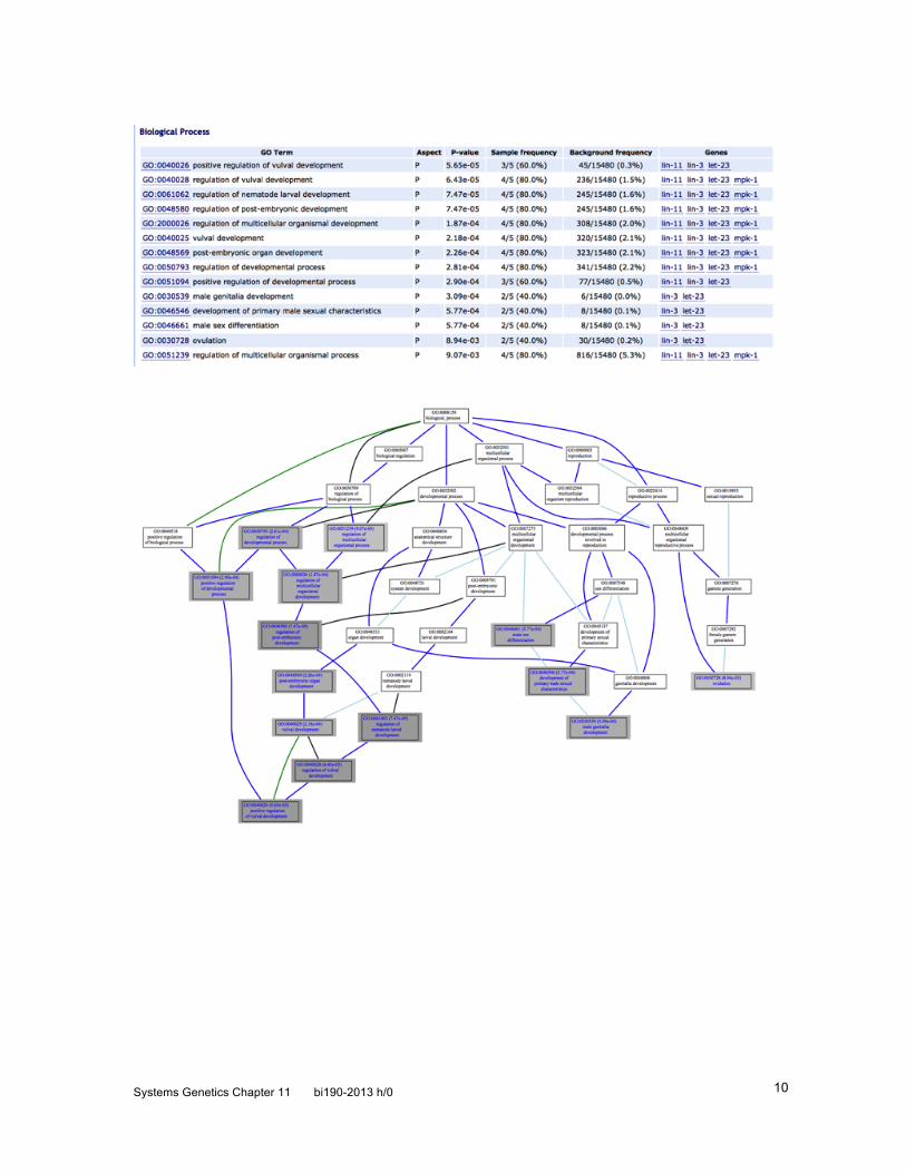
chapter 11: gene expressionbi190/sg11.pdf · systems genetics chapter 11 bi190-2013 h/0 !! 1...

Documents