chapter 11 embryomorphic engineering: emergent innovation...

Chapter 11Embryomorphic Engineering:Emergent Innovation ThroughEvolutionary Development

René Doursat, Carlos Sánchez, Razvan Dordea, David Fourquetand Taras Kowaliw

Abstract Embryomorphic Engineering, a particular instance of MorphogeneticEngineering, takes its inspiration directly from biological development to createnew robotic, software or network architectures by decentralized self-assembly ofelementary agents. At its core, it combines three key principles of multicellularembryogenesis: chemical gradient diffusion (providing positional information to theagents), gene regulatory networks (triggering their differentiation into types, thuspatterning), and cell division or aggregation (creating structural constraints, thusreshaping). This chapter illustrates the potential of Embryomorphic Engineering indifferent spaces: 2D/3D physical swarms, which can find applications in collectiverobotics, synthetic biology or nanotechnology; and nD graph topologies, which canfind applications in distributed software and peer-to-peer techno-social networks.In all cases, the specific genotype shared by all the agents makes the phenotype’scomplex architecture and function modular, programmable and reproducible.

This chapter is a condensed review version of references [16–22].

R. Doursat (B) · T. KowaliwComplex Systems Institute Paris Ile-de-France (ISC-PIF),CNRS and Ecole Polytechnique, 57-59, rue Lhomond, 75005 Paris, Francee-mail: [email protected]

C. A. SánchezResearch Group in Biomimetics (GEB),Universidad de Málaga, C/ Severo Ochoa 4, PTA, 29590 Malaga, Spain

R. Dordea · D. FourquetErasmus Mundus Masters in Complex Systems Science (EMMCS),Ecole Polytechnique, Route de Saclay, 91120 Palaiseau, France

R. Doursat et al. (eds.), Morphogenetic Engineering, Understanding Complex Systems, 275DOI: 10.1007/978-3-642-33902-8_11, © Springer-Verlag Berlin Heidelberg 2012

276 R. Doursat et al.

11.1 Evolutionary Development

Morphogenetic Engineering (ME), the topic of this book, concerns the design, orrather “meta-design”, of the self-organizing abilities of the elements of complex sys-tems toward functional architectures. This meta-design, however, should not exclu-sively rely on human inventiveness as in traditional engineering disciplines but mayalso involve an important automation part, essentially via an evolutionary search. Inthat sense, by combining not only self-organization and architecture but also evolu-tion, ME is very close to the tenets of evolutionary development, a recent and rapidlyexpanding field of biology nicknamed “evo-devo” [6, 8, 10, 11, 30, 40, 48, 58, 68].

11.1.1 Evo-Devo in Biology

In the variation/selection couple of evolutionary biology, “selection” has receivedmost of the honors while “variation” remained the neglected child. Darwin discov-ered the evolution of species, based on random mutations and nonrandom naturalselection, and established it as a central fact of biology. During the same period,Mendel brought to light the laws of inheritance of traits. In the twentieth century, hiswork was rediscovered and became the foundation of the science of genetics, whichculminated with the revelation of DNA’s role in heredity by Avery and its double-helix structure by Watson and Crick. Integrating evolution and genetics, the “ModernSynthesis” of biology has successfully demonstrated the existence of a fundamentalcorrelation between genotype and phenotype and between their respective changes:mutation in the first is causally related to variation in the second. Yet, 150 years afterDarwin’s and Mendel’s era, the nature of the link from genes to organismal forms,i.e., the actual molecular and cellular basis of the mechanisms of development, arestill unclear. How does a one-dimensional genome specify a three-dimensional ani-mal? [24]. How does a static, linear DNA unfold in time (regulation dynamics) andspace (cellular self-assembly)? What is the part also played by epigenetics? Thesequestions constitute the missing link of the Modern Synthesis and the main challengeof evo-devo.

While the attention was focused on selection, it is only during the past decade thatanalyzing and understanding variation (as the generation of phenotypic innovation)by comparing the developmental processes of different species, at both the embry-onic and the genomic levels, became again a major concern of biology. Researchersrealized that the genotype-phenotype pairing could not forever remain an abstractionif they wanted to understand the unique power of evolution to produce countlessinnovative structures—and, concerning Artificial Life and bio-inspired engineering,ultimately transfer this understanding to self-organized technological systems. Toquote Kirschner and Gerhart [40, p. ix]:

When Charles Darwin proposed his theory of evolution by variation and selection, explainingselection was his great achievement. He could not explain variation. That was Darwin’s

11 Embryomorphic Engineering: Emergent Innovation 277

dilemma. . . . To understand novelty in evolution, we need to understand organisms downto their individual building blocks, down to their deepest components, for these are whatundergo change.

Evo-devo casts a new light on the question still little addressed by today’s predom-inant gene-centric view of biology: To what extent are organisms also the product ofcomplex physicochemical developmental processes not necessarily or always con-trolled by complex underlying genetics? Before and during the advent of genetics, thestudy of developmental structures had been pioneered by the “structuralist” schoolof theoretical biology, which can be traced back to Goethe, D’Arcy Thompson, andWaddington. Later, it was most actively pursued and defended by Kauffman [38, 39]and Goodwin [30] under the banner of self-organization, argued to be an even greaterforce than natural selection in the production of viable diversity.

Recent dramatic advances in the genetics and evolution of biological developmenthave paved the way toward explaining morphological self-organization and sketchingan encompassing “generativist” theory of embryogenesis. The objective is to unifyorganisms beyond their seemingly “endless forms most beautiful” (in the words ofDarwin [7]) by unraveling the generic mechanisms that make them variations arounda common theme [68]. The variations are the specifics of the genetic and epigeneticinformation; the theme is the developmental dynamics that this information steers. Itcomprises the elementary laws by which the genome produces the very proteins thatcan further interpret it, controlling cell division, differentiation, adhesion and death,and ultimately producing an anatomy. On this keyboard, evolution is the ultimateplayer.

11.1.2 Evo-Devo in Artificial Life

Looking at the full evolutionary and developmental picture should also be a pri-mary concern of systems engineering and computer science when venturing into thenew arena of autonomous, distributed architectures. Evolutionary Computation (EC)techniques such as genetic algorithms or genetic programming, which were inspiredby evolutionary biology in its traditional modern-synthesis form, have like their nat-ural model principally focused on selection through virtual “genomic operators”,“fitness functions” and “reproduction rates”. As a consequence, the great majorityof these approaches rely on more or less direct and abstract mappings from artificialgenomes to artificial individuals, while including only little or no morphogenesis.

Therefore, one important goal of a new field of “Alife evo-devo” is to providethe computational foundation for a virtual re-engineering of the “strongly morpho-genetic” complex systems spontaneously produced by nature, such as biologicaldevelopment. To this aim, one must design a programmable and reproducible two-way indirect mapping between the local rules of self-assembly followed by the ele-mentary agents at the microscopic level (the genotype �), and the collective structureand function of the system at the macroscopic level (the phenotype �). Calculating


the transformation from � to � corresponds to developing an organism—while solv-ing the inverse problem of finding an appropriate � given a desired � (or family ofsimilar�’s), would be the challenge of an evolutionary search, whether goal-oriented,open-ended, or a mix of the two.

Mirroring the evo-devo paradigm in biological systems, new EC avenues need tostress the importance of fundamental laws of developmental variations as a prereq-uisite to selection on the evolutionary time scale of artificial systems [62]. From theEC viewpoint, it means an implicit or indirect mapping from genotype to phenotype.Fine-grained, hyperdistributed architectures similar to multicellular organisms (i.e.,many light-weight agents, as opposed to a few heavy-weight agents) might be in aunique position to provide the “solution-rich” space needed for successful selectionand spontaneous innovation through developmental modularity and composition.

11.1.3 From Embryogenesis to Embryomorphic Engineering

Putting in practice the above theoretical intentions, this chapter offers an overview ofa recent framework called Embryomorphic Engineering, founded in 2006 by RenéDoursat [16, 17] (who coined the term after “Neuromorphic Engineering”) to explorethe causal and programmable link from genotype to phenotype that is needed in manyemerging computational disciplines, such as artificial embryogeny [5, 46, 62], andapply it to innovative uses. Its endeavors as a bio-inspired computing technologyfollow those of biological evo-devo, and for this reason it could be equivalentlyreferred to as “Evo-Devo Engineering”. Embryomorphic Engineering works on twolevels in parallel: it consists of simultaneous genetic engineering (�) and functionalshape engineering (�), based on a common playground made of a multitude ofsmall agents capable of self-assembling into a particular organism. These agents areguided by the genetic instructions they carry, which parametrize and modulate thefundamental laws of biomechanical-like assembly and biochemical-like signalingthat they obey, creating appropriate context-sensitive rules.

The remainder of the text illustrates the potential of Embryomorphic Engineeringin different spaces: 2D/3D physical swarms, which can find applications in collectiverobotics, synthetic biology or nanotechnology; and nD graph topologies, which canfind applications in distributed software and peer-to-peer techno-social networks. Inall cases, the specific genotype shared by the agents makes the phenotype’s complexarchitecture and function modular, programmable and reproducible:

• Section 11.2 describes MapDevo (Modular Architecture by Programmable Devel-opment), the original and foundational 2D model of embryonic developmentbased on self-assembly, pattern formation, and genetic regulation (Fig. 11.1).Section 11.3 examines hand-made mutations of the genotypes of MapDevo organ-isms and their corresponding phenotypes, paving the way toward an evolutionaryversion of programmable development. It is followed in Sect. 11.4 by a study offunctional—not merely morphological—architectures, called fMapDevo, through


Fig. 11.1 The iterative 3-stage MapDevo growth cycle

a model of animated embryomorphic organisms immersed in a 3D physical envi-ronment.• After those 2D/3D models, which remained close to their biological inspiration

based on multicellular development, Sect. 11.5 presents ProgNet (ProgrammableNetwork Growth), an extension of MapDevo to nD graph topologies via a modelof autonomous network construction. There, nodes execute the same program inparallel, communicate and differentiate, while links are dynamically created andremoved based on “ports” and “gradients” that guide nodes to specific attachmentlocations. As the network grows, nodes switch different rules on and off, creatingchains, lattices, and other composite topologies. Finally, Sect. 11.6 introducesProgLim (Program-Limited Aggregation), a particular implementation of ProgNetin cellular automata, and Sect. 11.7 briefly concludes the chapter.

11.2 MapDevo: Modular Architecture by ProgrammableDevelopment

The spontaneous making of an entire organism from a single cell is the epitome ofa self-organizing and programmable complex system. Through a precise spatiotem-poral interplay of genetic switches and chemical gradients, an elaborate form is cre-ated without explicit architectural plan or engineering intervention. Embryomorphic


agent-based modeling and simulation attempt to understand and exploit these fun-damental morphogenetic mechanisms.

On the one hand, research in self-assembling (SA) systems, whether natural orartificial, has traditionally focused on pre-existing components endowed with fixedshapes [69]. Biological development, by contrast, dynamically creates new cells thatacquire selective adhesion properties and forms through differentiation induced bytheir neighborhood [72]. On the other hand, biological pattern formation (PF) phe-nomena [28, 42, 45, 50, 63, 73] are generally construed as orderly states of activityon top of a quasi-continuous and fixed 2D or 3D background of cellular substrate.Yet again, the spontaneous patterning of an organism into regions of gene expressionarises within a multicellular medium in perpetual expansion and reshaping. Finally,both phenomena (SA and PF) are often thought of in terms of stochastic events—whether mixed components that randomly collide during SA, or spots and stripesthat crop up unpredictably from instabilities during PF. Here too, these notions needsignificant revision if they are to be extended and applied to embryogenesis. Cells arenot randomly mixed but pre-positioned where cell division occurs. Genetic identityregions are not randomly distributed but highly regulated in number and position.

This section describes MapDevo (Modular Architecture by Programmable Devel-opment), the original and foundational 2D model of Embryomorphic Engineeringfirst published in [16–18]. It is a spatial computational simulation of programmableand reproducible morphogenesis that combines SA and PF under the control of anonrandom gene regulatory network (GRN) stored inside each cell of a swarm. Thedifferential properties of cells (division, adhesion, migration) are determined by theregions of gene expression to which they belong, while at the same time these regionsfurther expand and segment into subregions due to the self-assembly of differenti-ating cells. To follow an artistic metaphor [10], SA is similar to “self-sculpting”and PF to “self-painting”. The model can be construed from two different vantagepoints: either pattern formation on moving cellular automata, in which cells divideand spatially rearrange under the influence of their own activity pattern; or collectivemotion in a heterogeneous swarm, in which cells gradually differentiate and modifytheir interactions according to their positions and the regions they form.

In the next subsections, the motion of a homogeneous swarm of cells (pure SA)and the patterning by gradient propagation on a static swarm (pure PF) are introducedseparately. Then, these two components are combined to form reproducible growingpatterns (SA+ PF). The genetic control inside every cell guiding these arrangementsis also explained. Finally, this combination is repeated in modules (SAk + PFk)inside a larger, heterogeneous system to create complex morphologies by recursiverefinement of details.

Self-assembly by Division and Adhesion (SA) The original MapDevo modelconsists of a 2D swarm of cells with dynamically changing neighbor interactionscalculated by a Delaunay-Voronoi tessellation (Fig. 11.2). Each cell follows twomajor laws of cellular biomechanics in a simplified format: (i) cell division, codedby a uniform probability p for any cell to split into two, and (ii) cell adhesion, repre-sented by elastic forces derived from a quadratic potential V with resting length re,


Fig. 11.2 Deployment of a homogeneous swarm (SA). a Cell-to-cell interaction potential V similarto elastic springs. b Relaxation of a 400-cell swarm from an initially compressed layout. c Sameswarm viewed from its underlying mesh of pairwise interactions, obtained by Delaunay triangulationand pruning of links longer than r0. d Genetic SA parameters inside every cell (from [18])

hard-core radius rc, and scope of visibility r0, similar to collective motion models [31,66] but with zero velocity (no self-propulsion). These parameters are grouped into agenotype GSA. Laws of motion are derived from a spring-damper system with neg-ligible mass/inertia effects. Under potential V , starting from a compressed swarm,cells quickly relax to a resting state that forms a quasi-regular hexagonal mesh.

Propagation of Positional Information by Gradients (PF-I) Pieces of a jigsawpuzzle are defined not only by their position and shape but also by the “image”that they carry. In our self-organized swarm, this translates into state variables thatdetermine the PF activity inside each cell. The model distinguishes between twokinds of PF-specific state variables (i.e., signals that cells continuously exchangeand process): gradient variables (PF-I) and pattern variables proper (PF-II).

Gradient values (PF-I) propagate from cell to cell to establish positional informa-tion across the swarm [71]. For example, each cell contains a counter variable gW .The source cell of this gradient, denoted W , is characterized by gW = 0. It passesvalue 1 to neighboring cells, which in turn tell their neighbors to set gW to 2, and soon (Fig. 11.3). To give this isotropic propagation a specific direction, another localrule instructs each cell to retain only the smallest of the current counter value and thereceived values. The result is a roughly circular wave pattern of increasing gW coun-ters centered on source W . Together with W , three other gradients, E , N and S, con-tribute to form a 2D coordinate system via equatorial (midline) axes X = NS⊥ andY = WE⊥, which contain the cells where counter values cross, respectively: |gY =gN−gS| ≤ 1 and |gX = gW−gE | ≤ 1. Note that the four sources W , E , N , S positionthemselves, too, by “hopping” away from each other (i.e., passing a flag representingsource N to any neighbor with a higher S-gradient value, and vice-versa; same for Wand E). First defined by Lewis Wolpert [71], “positional information” is a fundamen-tal concept of biological development, and its natural chemical versions (morphogendiffusion and messenger-based signaling) are often translated into discrete coun-ters in artificial systems like this one, such as in Amorphous Computing [12, 49]and Spatial Computing [3, 4].


Fig. 11.3 Propagation of positional information (PF-I). a Circular gradient of counter values origi-nating from source cell W (circled in red; end points circled in blue). b Same gradient values viewedthrough a cyclic color map. c Opposite gradient coming from antipode cell E . d Set of midline cellsY = WE⊥ whose W and E counters are equal ±1. e Quasi-planar gradient gX = gW − gE . f, gFull coordinate compass with axis X = NS⊥ ≈ WE (adapted from [18])

Programmed Patterning by Gene Expression Levels (PF-II) Pattern values (PF-II)correspond to gene expression levels that are calculated on top of the (gX , gY ) gra-dient values to create different cell types (which in turn affect the SA behavior;see SA + PF integration below). This calculation relies on a gene regulatory net-work (GRN) inside each cell, whose weights constitute the genetic parameters ofthe PF process and are denoted by GPF (Fig. 11.4). The inputs of the GRN arethe morphogen/second-messenger proteins whose concentrations are encoded in thegradient values gX and gY . Thus the core architecture of the virtual organism is anetwork of networks, i.e., an irregular 2D lattice of identical GRNs locally coupledto each other via “chemical signaling” nodes (here, gX and gY ) [13, 47, 53].

The patterning process represents the emergence of heterogeneity, i.e., the seg-mentation of the swarm into “identity regions” corresponding to high expressionlevels of particular genes Ik of the GRN. A well-known example is the early stripingof Drosophila [8] controlled by a 5-layer hierarchy of segmentation genes along theanteroposterior axis (maternal genes, gap genes, primary/secondary pair-rule genes,and segment polarity genes). The present model relies on a 3-layer caricature of thesame principle along the two intersecting axes X and Y : (1) the bottom (input) layerof the GRN groups the two positional variables (morphogen concentrations) gX andgY ; (2) the middle layer groups “boundary” genes Bi , which segment the embryo intoroughly horizontal and vertical half-planes of strong and weak expression levels via2D step functions σ ; (3) the top (output) layer groups the identity genes Ik derivedfrom positive and negative products of the Bi ’s, i.e., various intersections of the Bi

half-planes.

Simultaneous Growth and Patterning (SA + PF) After describing the self-assembly of a non-patterned swarm (SA) and the patterning of a fixed swarm (PF),the embryomorphic SA and PF behaviors are combined to create growing patterns at


Fig. 11.4 Programmed patterning (PF-II). a Same swarm viewed under different color mapsrevealing the regions where cells’ internal variables gX , gY , Bi and Ik are highest (virtual equiv-alent of in situ hybridization in biology). b Consolidated view of all identity regions Ik fork = 1...9. c The GRN, denoted GPF, used by each cell to calculate its expression levels, here:B1 = σ(−1/3− gX ), B3 = σ(1/3− gY ), I4 = B1 B3(1− B4), etc. (adapted from [18])

every stage (Fig. 11.5). Cells continually adjust their positions according to the elas-tic SA constraints, while exchanging PF signals over the same dynamic links. Thisdual dynamics is guided by the combined genotype G = (GSA, GPF). Daughter cellsinherit all the attributes of mother cells, including G and the current internal PF vari-ables (gradient counters and gene levels). As for the SA variables (coordinates andadhesion/signaling links of the lattice), they are recalculated from a position close tothe original cell. Both sets of variables are updated as the newborn cell immediatelystarts contributing to the SA forces and the traffic of PF gradients, which maintainthe pattern’s consistency at all times in the swarm.

Modular, Recursive Patterning (PFk) Natural embryological patterns, however, donot develop in one shot but in numerous incremental stages [10]. An adult organ-ism is produced through modular, recursive growth and patterning. In Drosophila,regions of the embryo that acquire leg, wing or antenna identity (called “imaginaldiscs”) start developing local coordinate systems of morphogen gradients to supportthe prepatterning and construction of the planned organ [8]. Correspondingly, thepresent embryomorphic model includes a pyramidal hierarchy of network modulesable to generate patterns in a recursive fashion (Fig. 11.6). First, the base networkG0

PF establishes the main identity regions as above, then subnetworks GkPF triggered

by the identity genes Ik of G0PF further partition these regions into smaller, special-

ized compartments at a finer scale. This “trigger” is based on usual gene regulationmechanisms, whereby proteins produced by Ik bind to the regulatory sites of genesBk

i in the upper layer and are necessary to promote their expression. Fractal pattern-ing has also been explored in generative algorithms such as “L-systems” [52, 61].These algorithms, however, are most often self-similar and rely on symbolic rules andexplicit geometry. In contrast, MapDevo is a dynamical system of physicochemical


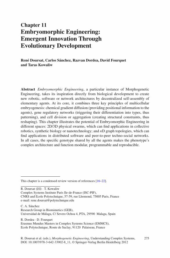
Fig. 11.5 Simultaneous growth and patterning (SA + PF). a Swarm growing from 4 to400 cells by division. b Swarm mesh, highlighting gradient sources and midline axes.The gradients and the whole pattern are continually maintained by source migration,e.g., N moves away from S and toward WE⊥ (same with the other three sources).c Cell B created by A’s division quickly contributes to SA forces and PF traffic.d Combined genomes inside each cell (adapted from [18])

Fig. 11.6 Modular, recursive patterning (PFk ). a A 9-region swarm, as in Fig. 11.4b. b Cells atthe border between two domains are highlighted with yellow circles. c These border cells becomenew gradient sources (red circles) inside certain identity regions at a lower scale. d Missing bordersources arise from the ends (blue circles) of other gradients. e, f Subpatterning of the swarm insideI4 and I6. g Corresponding hierarchical GRN: GPF = {G0

PF, G4PF, G6

PF} (from [18])

interactions among a multitude of units (a distinction also made in cognitive sciencebetween Artificial Intelligence and Neural Networks).

Modular, Anisotropic Growth (SAk) So far missing from the model is a truetopological deformation dynamics, or “morphodynamics”, that can confer non-trivial shapes to the organic system beyond mere blobs. To this aim, cells mustbe able to diversify their SA characteristics, depending on their PF type andspatial position—thus closing the feedback loop between genetics and geome-try [11]. In particular, they have to exhibit nonuniform, anisotropic cell division


Fig. 11.7 Modular, anisotropic growth (SAk ). a Genetic SA parameters are augmented withrepelling V values r ′e and r ′0 used between the growing region (green) and the rest of the swarm(gray). b Daughter cells are positioned away from the neighbors’ center of mass. c Offshoot growthproceeds from an “apical meristem” made of gradient ends (blue circles). d Cyclic coloring of thegradient underlying this growth (from [18])

(varying p) and differential adhesion (varying V ). For example, in our artificialmodel, the growth of limb-like structures can be achieved by a coarse imita-tion of meristematic plant offshoots (Fig. 11.7). In this process, only the tip or“apical meristem” of the organ is actively dividing at any time (whereby cellsforming the tip self-identify as being the local maxima of the gradient generatedby the base of the limb). Moreover, potential V is defined to be attractive onlyamong cells within the limb region, while it becomes repelling (i.e., r0 ≤ re,see Fig. 11.2a) between the limb and other areas. Just like inhomogeneous divi-sion, differential adhesion is an essential ingredient of complex shape formation[34, 44].

Modular Growth and Patterning (SAk + PFk) Putting everything together, fullmorphologies can develop and self-organize from a few cells (Fig. 11.8). Thesemorphologies are complex, programmable and reproducible: they are architecturallycomplex because they can be made of any variety of modules and parts that are notnecessarily repeated in any periodic or self-similar way; they represent programmablephenotypes because they emerge from a same given genotype carried by every cellof the swarm; they are reproducible, because their structure and shape are not left tochance but tightly controlled by the genotype.

Naturally, the exact positions of the cells at the microscopic level are still random,but not the positions of the mesoscopic and macroscopic regions that they form.Moreover, the modularity of the phenotype is a direct reflection of the modularityof the genotype. The hierarchical SA and PF dynamics recursively unfolds insidethe different regions and subregions that it creates. Each module Gk = (Gk

SA, GkPF)

can be reused by exact duplication, but can also diverge from other blocks throughdifferent internal genetic SA and PF parameters, potentially giving each region adifferent morphodynamic behavior and a different gene activity landscape. Duplica-tion of gene modules followed by divergence of these copies is the basis of serialhomology, a major evolutionary mechanism in nature exemplified by vertebrae, teeth,or digits [8]. Here, the integration between SA and PF is controlled by the identity


Fig. 11.8 Modular growth and patterning (SAk+PFk ). a Example of a three-tier modular genotypegiving rise to the artificial organism on the right. b Three iterations detailing the simultaneous limb-like growth process (Fig. 11.7) and patterning of these limbs during execution of the middle tier(modules 4 and 6). c Main stages of the complex morphogenesis process, showing full patterns afterexecution of the bottom, middle and top tiers (from [18])

genes Ik : their corresponding nodes in the GRN switch on the execution of subor-dinate modules Gk (Fig. 11.6g), i.e., their gene expression activity (parametrizedby Gk

PF) to create new local segmentation patterns, and their mechanical behavior(parametrized by Gk

SA) to create new morphodynamical processes.

11.3 Toward an Evolutionary MapDevo Through Variation

This section presents experiments involving hand-made mutations of the genotypesof MapDevo systems and their corresponding phenotypes (first published in [19]).For now, these systems are purely developmental and do not serve a specific purpose.There is no organism fitness or selection-based evolutionary search. These importantaspects are included in ongoing projects, which will be previewed in Sects. 11.4and 11.6. Here, we exclusively focus on variation to illustrate the link betweengenotype and phenotype, and the programmable and predictable effect that changesin the former can have on the latter via self-organization—in which modularity is anessential condition of future evolvability [6, 58, 67].

The figures of this section show several simulation examples of modular embryo-genesis and how certain mutations in the genotype correlate with quantitative orqualitative changes in the phenotype. The organism of Fig. 11.9a is taken as the ref-erence or “wild type”. Its genotype is composed of two layers with one module each:a base module establishing the body plan (lower module) and a specialized modulein charge of growing a simple limb-like appendage (upper module). The latter is exe-cuted twice, in the left and right regions of the body, switched on by identity genesI4 and I6 (like in Fig. 11.6a). As just described in Sect. 11.2, each module consists oftwo types of genomes: a self-assembly genome GSA, encoding how cells divide andspread spatially, and a pattern formation genome GPF, encoding how cells acquiretheir types. To simplify the figures, the GRN that constitutes GPF is not displayed


Fig. 11.9 Simulation trials showing quantitative variations. a–c Varying limb thickness by modi-fying the GRN weights and thresholds. d–f Varying length and size of limbs and body by stoppingcell division earlier or later (from [19])

in its entirety; instead, only the type of checkered pattern that it produces (explainedbelow) and the module-switching identity genes are sketched.

Quantitative Variation of Limb Thickness by GRN Weights (PF) In Fig. 11.9b,the wild-type organism has been affected by a “thin-limb” mutation of the bodyplan. Although not shown, some weights and thresholds of the base GPF have beenmodified in such a way that they now create a checkered pattern with a narrowercentral row (displacing the Bi gene domains of Fig. 11.4a). This gives less spacefor the limb buds to grow, hence making them thinner. The reverse, “thick-limb”mutation is shown in Fig. 11.9c, with coefficient 2. This is a good example of thecompactness of the developmental genotype [26, 62] and its large-scale effect on thephenotype: slightly varying the sensitivity of a couple of genes can already result insignificant morphological changes.

Quantitative Variation of Limb Length by Division Signals (SA) By modifyingthe division rate and/or the stop conditions of proliferation, the size of various parts ofthe embryo can also be modulated. For example, in Fig. 11.9d and e, cell proliferationis regulated in the limbs. Here, it is achieved by stopping division when the gradientvalues of the tip cells (blue circles in Fig. 11.7) reach a specific value g′, respectivelysooner (g′ = 10) and later (g′ = 40) than the wild type (g = 15). In Fig. 11.9f,both body plan and limbs stop growing beyond gradient value g′ = 8, producing aphenotypic shape that is proportionally smaller than the wild type. Note that similareffects can also be achieved by decreasing or increasing the probability of divisionp, while keeping the stop gradient values constant (see Fig. 11.10c).

Structural Change of Limb Position by Module Switching In Fig. 11.10, themodularity of the limb component is demonstrated through various mutations rem-iniscent of experiments on biological organisms such as Drosophila. The identitygenes marking the regions (“imaginal discs”) responsible for the growth of a specific


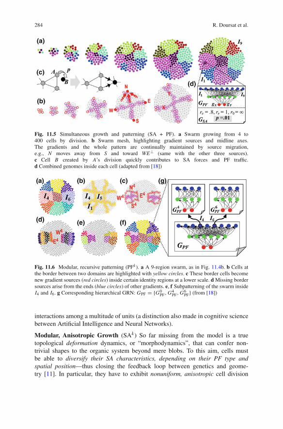
Fig. 11.10 Simulation trials showing structural variations. a–c Changing limb configuration byswitching the limb-triggering genes and/or duplicating the limb module (from [19])

Fig. 11.11 More structuralvariations. d, e Adding limbsby body plan expansion(from [19])

appendage [8, 10] can be literally turned on or off in new regions with respect to thewild type of Fig. 11.9a. For example, in Fig. 11.10a, a virtual case of “antennapedia”,i.e., the ectopic growth of a leg where there should be an antenna, is obtained byconnecting a new identity region to the limb module, here region I2 instead of regionI6. This means rewiring the GRN of GPF to reflect the fact that the regulatory sites ofthe limb genes on the DNA have mutated and now accept gene I2’s proteins as pro-moters instead of gene I6’s proteins. In the three-limb mutation of Fig. 11.10b, theseregulatory sites have been duplicated before mutating, accepting gene I2 in additionto gene I6 (not just in replacement), so that the limb module is now executed threetimes in three different regions instead of twice.


Structural Duplication and Divergence, or “Serial Homology” Later in the courseof evolution, similar copies of the same organ can diverge and acquire specializedcharacteristics, as Fig. 11.10c illustrates. In this scenario, three copies of the entirelimb module were produced by duplication as in Fig. 11.10b. Afterwards, thesecopies mutated independently from each other, e.g., by adopting different cell divi-sion rates p′, which created shorter or longer limbs. Serial homology is the namegiven to this major evolutionary process resulting from duplication followed bydivergence [7, 40]. Biological organisms often contain numerous repeated parts intheir body plan. This is most striking in the segments of arthropods (several hun-dreds in millipedes; see the simulated “biomorphs” of [14]) or the vertebrae, teethand digits of vertebrates. After duplication, these parts tend to diversify and evolvemore specialized structures (lumbar vs. cervical vertebrae, canines vs. molars, etc.).Homology exists not only within individuals but also between different species, asclassically shown by comparing the forelimbs of various tetrapods from the bat to thewhale. Thus homology should also be explored as an important principle of artificialself-developing systems.

Structural Addition of Limbs by Body Plan Expansion In the scenario ofFig. 11.11d and e, new limbs are generated not by reusing the same body plan differ-ently (Fig. 11.10a and b) or by duplicating the limb module (Fig. 11.10c), but ratherby expanding the GRN of the base GPF in order to create new regions of gene identitythat can host additional limb growth. Here, the embryo’s geography has expandedfrom a 3 × 3 = 9-type checkered pattern to a 5 × 3 = 15-type (Fig. 11.11d) and a9× 3 = 27-type pattern (Fig. 11.11e). The SA part of the body plan is also slightlymodified to accommodate these new regions. It assumes an oval shape resulting froma nonuniform distribution of the division rate p that elongates the body along the Yaxis (see Fig. 11.3), i.e., greater toward the N and S poles and lower in the middle.

Structural Addition of Digits by Modular Hierarchy Finally, along the same prin-ciples, Fig. 11.12 shows a few simulation trials of three-tier organisms. Figure 11.12ais the new wild type. After the usual development of two limbs from the 3× 3 bodyplan, extra “digits” now grow from these limbs, guided by the top module of the hier-archical genotype. To make room for these digits, limbs have expanded their internalpattern from 1×1 to 2×4 (see previous paragraph). Figure 11.12a presents a doublebilateral symmetry, with respect to both horizontal and vertical axes. Figure 11.12c isa further mutation of Fig. 11.12b, in which region I6’s limb has accelerated its growthand expanded its checkered pattern to support the development of two new digits,whereas, on the contrary, region I4’s limb has continued to regress back to a prim-itive “stump”. Figure 11.13 paints a possible phylogenetic tree that includes all thespecies simulated in this section (dashed branches suggest “convergent” speciationpathways).

Naturally, beyond these proof-of-concept simulation trials, a more systematicexploration is needed. Further work needs to be done on how an embryomorphicsystem can spontaneously evolve, i.e., how it can be randomly varied and non-randomly selected based on its success in performing certain tasks. Toward this


Fig. 11.12 a–c Adding digits to the limbs via a third tier in the modular hierarchy of the genotype(from [19])

Fig. 11.13 A phylogenetictree (from [19])

objective, different selection strategies are possible, whether focusing on prespecifiedforms, prespecified functions, or allowing open outcomes.

When selecting for form, a hard reverse engineering problem must be addressed:given a desired phenotype, what is the genotype that can produce it? While determin-


istic phenotype-to-genotype “compilation” is possible in limited cases [49], parame-ter search is generally difficult. With a fitness criterion rewarding only a specifictarget shape, solutions in genomic space are likely to be few and far between, ifnot reduced to a unique spot. In this situation, a classical approach is to define a“shape distance” as an increasing function of favorable, stepwise mutations. It isconjectured here that this kind of gradual search might actually benefit, not suffer,from the high genotype dimensionality of an embryomorphic model, compared tothe direct genotype-phenotype mappings of most genetic algorithms. HierarchicalGRNs might be better at providing the fine-grained mutations required by the “gentleslope” search toward increasingly sophisticated innovation [14, 51]. Complex sys-tems inherently have greater variational power, as they allow combinatorial tinkeringon highly redundant parts.

However, beside gaining self-repair properties, why constrain a self-assemblingsystem to produce a predefined shape? More benefits might come from such systemsby selecting them for function while leaving complete freedom of form. Gradualoptimization could rely on a distance of performance to predefined goals, instead ofshapes, allowing the most successful candidates to reproduce faster and mutate. Func-tional selection under free form has often been tried in evolutionary robotic systems[41, 43], but there it was based on non-developmental, direct genotype-phenotypeencodings. Again, it is hypothesized here that a larger number of microscopic agents,such as in multicellular embryogenesis, would be more favorable to a successfulfunctional search due to their collective combinatorial abilities.

Finally, in a third scenario, specifications can be diversified and relaxed to the pointof being open to surprise and harvesting unexpected but useful organisms from a“free-range menagerie” (see for example “evolutionary swarm chemistry” [57]). Ulti-mately, reconciling the antagonistic objectives of spontaneity and purpose will prob-ably hinge on two complementary aspects: (a) finer-grained variation-by-mutationmechanisms yielding a larger number of search paths and (b) looser selection criteriayielding a larger number of fitness maxima. With more search paths covering morefit regions, evolution is more likely to find good matches.

11.4 Functional MapDevo by Animation in 3D

While the task of “meta-designing” laws of artificial development inspired from biol-ogy is already challenging, it only constitutes the first part of the EmbryomorphicEngineering effort. Once a self-developing infrastructure is mature, what other com-puting and behavioral capabilities can it support? What do its “cells” (agents) and“organs” (regions) actually represent and achieve in practice? In biological organ-isms, although cell physiology often partakes in development (e.g., electrical signalsof neurons guiding synaptogenesis), there seems to be a broad distinction betweendevelopmental genes and the rest of the genome. In computing systems, these twomodes could also be separated into two different sets of state variables. After reach-ing developmental maturation, and while still fulfilling maintenance and self-repair


tasks, morphogenetic SA and PF activity (division, position information and pat-terning signals) would give way to another type of activity subserving functionalcomputation. Obviously, the type of computation entirely depends on the nature ofthe agents: processor-carrying nano-units, software agents, robot parts, mini-robots,synthetic bacteria, and so on.

In fact, the problem is the opposite in many computing domains: there is a demandfor precise self-formation capabilities in distributed systems made of existing func-tional agents. A variety of morphogenetic-like approaches have been proposed forsuch applications. For example, Amorphous Computing has set the stage for a myr-iad of micro-processors containing the same instructions to self-organize without anexact blueprint map or functional reliability, unlike traditional VLSI [1, 12, 49]. Self-assembling components can also represent mobile sensors and actuators in complexself-managing networks [3, 4]. In software applications (servers, security), a soci-ety of small-footprint software agents could diversify and self-deploy to achieve adesired level of application functionality and service (e.g., “immune” security [33]).It is also an important challenge in complex “techno-social networks” made of myr-iads of devices, software agents, and/or human users, which use only local rules andpeer-to-peer communication to achieve a collective function [23] (see Sect. 11.5). Incollective robotics, too, whether articulated parts of reconfigurable devices [29, 35,41, 43], or mobile formations of mini-robots [9, 32, 70], there is a need for complexbut controllable morphologies.

This section describes preliminary work toward such a goal through a modelof animated MapDevo organisms immersed in a 3D physical environment, calledfMapDevo [21]. The developmental process follows the exact same principles as the2D model of Sect. 11.2 (SA by elastic forces, PF-I by gradient propagation, PF-IIby gene expression). In addition, after development, mature organisms are able togenerate movement by contracting adhesion links between “muscle” cells, whileother cells have differentiated into “bones” and “joints” to support and articulate thebody’s structure. Finally, by interacting with a virtual physical world, made of a rigidfloor, simple objects and a gravitational field, creatures can exhibit locomotion andprimitive behavior. This project constitutes an original demonstration of a genuinelyevo-devo Alife system, in which self-organization is not only programmable butfunctional and evolvable. We summarize below the main features and novelties ofthis project compared to MapDevo.

Body Growth in 3D Space We use the Open Dynamics Engine (ODE) to imple-ment the embryomorphic development and behavioral dynamics of the organisms in3D. Like the 2D version, cells are modeled as point-like elements (here representedby small spheres, Fig. 11.14) and neighborhood relationships are calculated by a 3DDelaunay triangulation (Fig. 11.14e) from which long links are removed above a cut-off distance. As before, mechanical SA forces are elastic links between neighboringcells, and in the first stage—the growth of the body—cell division is characterized bya uniform probability and random orientation (visualized with vectors, Fig. 11.14f).Gradient propagation PF-I (Fig. 11.14g) is triggered by three pairs of source cells,North-South, West-East, and Top-Bottom (Fig. 11.14a), which place themselves as


Fig. 11.14 Simulation of body growth in 3D space. a The 6 original source cells inside a small ballof cells after a few divisions at iteration t = 25. b–d Successive growth states at iterations t = 150,400 and 700: 27 cell-type regions have formed under a 3×3×3 checkered gene expression pattern.e Detail of the mesh of neighborhood links calculated by 3D Delaunay triangulation. f Detail of therandom division vectors in each cell: norms represent probabilities, orientations are perpendicularto cleavage planes. g East gradient gE from the E source, displayed in red–white shading. h A thickequatorial plane (in red) corresponding to |gW − gE | ≤ 3

Fig. 11.15 Simulation of single limb development in 3D. a–d Successive states. a′–c′ Correspond-ing division field: the body has halted its growth (nullifying all division vectors inside), while in thelimb the division probability is 0 everywhere except at the local North tip (gN ≤ 3), where its ori-entation is South→North. e Detail of the division field at the tip. f The three pairs of self-positionedsources inside the limb (showing axes, not actual links), with South at its root and North at its tip

usual by hopping away from each other, i.e., navigating the opposite gradients uphill.Regional differentiation PF-II (Fig. 11.14b–d) results from the execution of a geneticprogram, whose output depends on the input gradients in each cell. In this model,however, the program is not necessarily a GRN but can be in symbolic format, suchas logic rules (e.g., “if |gW − gE | ≤ 3 then switch on the red gene”, Fig. 11.14h).

Modular Limb Growth, Homology and Divergence In a second stage, limb growth(Fig. 11.15a–d) proceeds in the same way as the 2D version, by relying on a het-erogeneous field of cell division probability and orientation (Fig. 11.15a′–c′), which


Fig. 11.16 Fully developed 4-legged organism. a Standard sphere-based multicellular view fromunderneath. b Corresponding division vector field, null in the limbs except at their tips. c Geneticprogram G executed by all cells, comprising three modules: a body module (uniform field of divisionprobability, 27 cell types), a short-limb module (tip-area division field, 2 subtypes, high link cutoff),and a long-limb module (small link cutoff). Each limb module is triggered in two different regionsof the body, creating a total of four legs. d Profile view of the creature when positioned on the floor

is calculated as a function of the local gradients inside the limb. In the examplebelow, cell division is zero everywhere except at the North tip, where its orientationis South→North (Fig. 11.15e, f). As in the 2D model, the same “homologous” limbmodule of the genotype can be reused to develop several limbs from different “imag-inal” regions of the body (Fig. 11.16). Then, evolutionarily “divergent” versions ofthat structure can be created by varying, for example, the link cutoff distance: a highvalue makes cells more likely to remain linked as neighbors, hence cluster togetherdue to the elastic attraction and create more compact, shorter limbs. Conversely, alower cutoff value tends to detach more cells from each other, hence let them spreadout and make longer limbs. In Fig. 11.16, the developed organism possesses onepair of short limbs and one pair of long limbs. In sum, each module of the organism(body, limbs, etc.) represents an autonomous domain of space in which local gradi-ents are mapped to various fields of developmental and structural parameters, suchas division vectors, cell types, link cutoff value (and stiffness coefficient: see next),via a local genetic program (Fig. 11.16c).

Bones, Joints, Muscles: Structural Differentiation and Dynamics In the embry-omorphic paradigm, the genotype-guided development of an organism not onlyprovides a reproducible overall shape, but can also equip this shape with built-in structural features that confer it specific mechanical properties. In Figs. 11.16and 11.17, for example, a few cells at the root of the limbs (where they attach tothe body) have differentiated into “muscles”, while others have become “bones” and“joints” inside the limbs. Computationally, this amounts to adding various Booleanfields—functions of the local gradients, like the division and type fields—to eachgenetic module (Fig. 11.16c). Here, the muscle field corresponds to a cylindricalsection of the limb’s root, e.g., where gS ≤ 5 (pink regions in Fig. 11.16a and d to becontrasted with the purple tips), while the bone field is 1 only along some thin South-North path on each limb and inside a small cluster at the center of the body. Linktypes are then simply deduced by connecting neighboring cells of identical types: forexample, the bone links are formed exclusively between bone cells (white edges in


Fig. 11.17 Structural differentiation and dynamics. a The grown organism contains a skeleton madeof differentiated “bone” cells and rigid links connecting them (displayed in white). b Experimentwhere all other links (the “flesh” in red) have been dissolved, showing the stability of the nakedbone structure under gravitational pull. c Opposite experiment where bone differentiation was turnedoff: the organism spreads on the floor like a starfish. d–g Locomotion and ball-kicking behavior,achieved by stimulating and contracting the “muscle” regions (pink roots of the limbs) in specificsubregions at specific time intervals—a coordination and control program that would be typicallythe task of a central nervous system

Fig. 11.17a, b). In this case, for a link to turn into “bone” means to become rigid, i.e.,acquiring a virtually infinite spring coefficient, so that it maintains a fixed spatial rela-tionship between its two extremities. The net effect is that a connected bone structureforms a “skeleton” that can support the whole organism and keep it standing on thefloor under gravitational pull. The skeleton’s stability can be revealed by “dissolvingthe flesh” around it as in Fig. 11.17b. Its usefulness can also be demonstrated byturning off bone differentiation, after which the softened organism collapses on thefloor in a spread-out posture resembling a starfish (Fig. 11.17c).

Behavioral Performance and Evolution Finally and most importantly, once themechanical features of cells and links have been established by development, theorganism is immersed in a physical environment where it can exhibit locomotionand other types of behavior. In Fig. 11.17d–g, it is shown walking on the floor andkicking a ball. Without going into details here, this is essentially achieved by con-tracting the muscle regions (pink roots of the limbs) periodically and nonuniformlythrough “stimulus” fields applied to specific subregions at specific time intervals—acoordination and control program that would be typically the task of a central nervoussystem, itself subject to evolutionary changes. For more information on this model,the reader is referred to upcoming publications such as [21].

In sum, the fMapDevo model offers a complete morphogenetic machine that cantransform by development a genotype G (Fig. 11.16c) into a functional phenotype(Fig. 11.16d). Metaphorically, G is the music roll of this mechanical organ, throughwhich evolution can play different original tunes, i.e., produce different innovativearchitectures.


11.5 ProgNet: Programmable Network Growth

After the foundational 2D/3D embryomorphic models of the MapDevo family(Sects. 11.2–11.4), which remained close to their biological inspiration based onmulticellular development, this part presents an extension to “nD” graph topologies.In this original project of programmable network self-construction and dynamics,called ProgNet (first published in [22]), neighborhood relationships between nodesare no longer necessarily a consequence of their proximity in Euclidean space. Yet,the overall challenge remains the same: design or evolve a ruleset that the individualagents of a multi-agent system can follow to independently create connections witheach other, such that the end result is an intended functional architecture.

With information and communication technologies (ICT) pervading everydayobjects and infrastructures, today’s Internet, so far playing the role of a communica-tion highway, is envisioned to become in the near future an “Internet of Things”, i.e.,a vast and hybrid complex network that will seamlessly integrate the physical andthe virtual worlds. It will enable the spontaneous creation of collaborative societiesof otherwise separate systems, both mobile and static, referred to as “cyber-physicalecosystems” (CPE) [64]. Examples will include self-reconfiguring manufacturingplants, self-stabilizing energy grids, self-deploying emergency taskforces [65], andself-growing autonomic applications [15]. What they will all have in common isa myriad of devices, software agents, and human users, dynamically building andreconfiguring their own network structures on the sole basis of local rules and peer-to-peer communication [23].

In this context, the ability to form specific connections by “programmed attach-ment” (as opposed to random connections by “preferential attachment” [2]) in adecentralized, self-organized way, would be of great benefit to a number of real-world situations where networking accuracy and reliability is important. Here, agentsare called “nodes” and represent, for example, human users equipped with wirelessdevices such as personal digital assistants (PDAs), or software agents acting as prox-ies for physical machines and other resources that need to function together.

The basic mechanisms of self-constructing networks in ProgNet are explained inthe following subsections from an abstract viewpoint. We start with elementary chainsand continue with more complicated, composite architectures, including branchingand stochastic redundancy. Nodes come in one by one and attach to the growingstructure toward the goal of building a particular topology. They communicate witheach other and execute the same program, but also gradually differentiate accordingto local and limited positional information in the form of discrete “gradients”, similarto MapDevo. The self-assembly program carried by each node includes routines forthe exchange of messages, the opening and closing of attachment ports and thedynamical creation or removal of links. Ports, gradients and other state variablesguide new nodes to specific locations in the developing network. As the networkexpands and node positions change, nodes adapt by switching different rule-subsetson or off—analogous to gene promotion/repression in DNA—thus triggering thegrowth of specific structures.


Fig. 11.18 Self-assembly of a simple chain. a The five main steps leading to a 5-node chain.Through the link creation routine L , incoming nodes attach to either open ports, X or X ′ (in darkblue), of the forming chain. When a link is created, its ports become “occupied” (in light blue)and gradient values are updated in all nodes (see b). When the chain length is 5, all open ports areclosed (in gray; see c). b Detailed substeps of the value-passing gradient update routine Gr . c Portmanagement routine P , the core and only evolvable component of genotype G in each agent: here,the ports of a node are instructed to close when x + x ′ = 4, i.e., length is 5 (adapted from [22])

Constructing Simple Chains Chains are the simplest self-assembling structures.In this first scenario, nodes possess two ports, X and X ′, and two correspondinggradient values x and x ′ (Fig. 11.18). Ports can be “occupied” (linked to other nodeports) or “free” (not linked), while free ports can be “open” (available for a link)or “closed” (disabled). New nodes that just arrived in the system’s space, or nodesthat are not yet connected, have both ports open and gradients set to 0. A new nodej can create a link with an existing node i only through a pair of complementaryopen ports, here X and X ′, with one link per port. Thus the only two possible linksbetween i and j are X ′j ↔ Xi or X ′i ↔ X j . Upon attachment, gradient valuesare immediately updated according to the following rules: (a) a free port alwaysmaintains its value at 0 (gradient source), and (b) assuming that it was link X ′i ↔ X j

that was created, value x is sent out in the direction X ′i → X j with an increment of+1 so that x j = xi + 1, while x ′ is sent out in the opposite direction X ′i ← X j sothat x ′i = x ′j +1 (swap i and j if the other link was created instead). This is similar tothe gradient propagation rule of the embryomorphic model presented in Sect. 11.2.

Figure 11.18 shows the self-assembly of a short chain. A new node can connectto any available open and complementary port at random, including the most recentand oldest nodes of the chain: all potentially valid links (here, two at any time) havean equal probability of being formed. The gradient counters keep track of the nodes’positions in the chain. This allows, for example, to build chains of a fixed length n byclosing any remaining open ports as soon as x + x ′ = n− 1. Again, as mentioned inSect. 11.2, discrete counter increments are also the method of choice for spreadingpositional information in other spatially extended paradigms [3, 4, 12, 49]. In thepresent model, the role of the gradient source can be transferred to another node,thereby shifting gradient chains in successive corrective waves, as nodes continu-ally communicate with each other to adjust their counters. Figure 11.18b shows an


Fig. 11.19 Sketch of a programmed branching scenario. a, b Beginning of chain a (ports and linksin blue). c Branch b starts to grow (orange). d Two alternative next steps. e Chain b stops growingat length 3. f Final developed structure, including a 4-node branch c (green). g This exact networkis prescribed by the port management program P carried by each node (from [22])

example of a step-by-step decomposition of a gradient update after a new node hasconnected to the chain (dashed circle to the left).

In sum, all nodes carry the same program, genotype G, which comprises threemain routines: gradient update (Gr ), port management (P), and link creation (L):

• The gradient update routine, denoted Gr to distinguish it from G, was explainedabove: it consists of generic code that provides nodes with the positional informa-tion that they need to make further decisions, and is used in all network structures(see next sections).

• The port management routine P (Fig. 11.18c) contains the heart of the logicspecific to the topology of a target architecture—chain, lattice, or any complicatedcomposite graph. For example, in the case of a 5-node chain, P simply commandsa node to shut its ports whenever x + x ′ = 4 (the “open” and “close” commandsapply only to free ports, and are ignored by occupied ports).

• Finally, the link creation routine L (Fig. 11.18a) is also generic logic that promptsnew nodes to pick one of the open ports of the network at random to make a newconnection.

Routines Gr and P are executed only by the nodes that are already involved in thenetwork, paving the way for newcomer nodes to execute routine L . In the remainderof the text, we focus on P , as it is the only variable and evolvable part of the genotypeG (while Gr and L are stereotyped and fixed).

Branching and Modular Structures by Local Gradients More complicated struc-tures can then develop by composing multiple chains and lattices. To allow thecreation of modules with their own identities and local positional information, onecan find again inspiration from biology, in particular the concepts of modularity and


Fig. 11.20 Simulation trials of programmed branching structures. a A main chain (horizontal,here) branches off into two smaller chains at points where the x gradient values respectively reach2 and 4. Nodes show here a unique ID number, which is not playing any role in the attachmentdynamics, while ports (represented by small rectangles attached to the nodes) contain the gradientvalues. Every node carries all three pairs of ports (blue, orange, green) but uses only 1, 2 or 3single ports (resp. at chain extremities, middles, and junctions). b Another example of chain (inblue) branching off into a red chain at x = 3 and a green chain at x = 5. Here, the layout followsa force-based algorithm and integer gradient values are visualized by color shading (from [20]). cExample of a complex programmed network integrating a branching chain structure with clusterformations (from [22])

homology that are central in evo-devo [8, 40, 48] (see Sect. 11.3). Modules are similarto “limbs” that have distinct morphologies and geographies. They are implementedhere by distinguishing between chain segments with independent coordinate systemsbased on different “tags” a, b, c, etc. To start with a simple example, a new chaincan branch off from the middle of another chain (Fig. 11.19). The gradient portsin the initial chain of the system are denoted by (Xa, X ′a), while the ports of thebranches will be (Xb, X ′b), (Xc, X ′c), etc. Accordingly, routine L is modified so thatlinks cannot be created between ports with different tags.

In the elementary scenario of Fig. 11.19, when the third node has attached (i.e.,when xa = 2), the P routine commands that a new pair of ports (Xb, X ′b) be createdon that node and only port X ′b be opened (Fig. 11.19c). Afterwards, new nodescan attach to either open port, X ′a (lengthening the initial chain) or X ′b (starting thenew branch; Fig. 11.19d). Under the right set of constraints, generally imposingunidirectional attachment (e.g., always to X ′), the order of node attachment doesnot influence the final structure. Actual simulation trials of self-organized branching


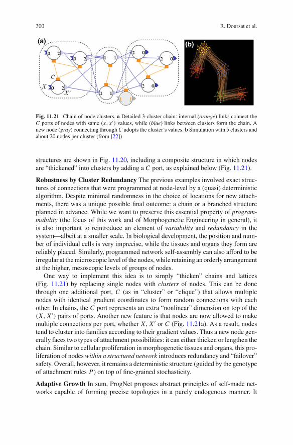
Fig. 11.21 Chain of node clusters. a Detailed 3-cluster chain: internal (orange) links connect theC ports of nodes with same (x, x ′) values, while (blue) links between clusters form the chain. Anew node (gray) connecting through C adopts the cluster’s values. b Simulation with 5 clusters andabout 20 nodes per cluster (from [22])

structures are shown in Fig. 11.20, including a composite structure in which nodesare “thickened” into clusters by adding a C port, as explained below (Fig. 11.21).

Robustness by Cluster Redundancy The previous examples involved exact struc-tures of connections that were programmed at node-level by a (quasi) deterministicalgorithm. Despite minimal randomness in the choice of locations for new attach-ments, there was a unique possible final outcome: a chain or a branched structureplanned in advance. While we want to preserve this essential property of program-mability (the focus of this work and of Morphogenetic Engineering in general), itis also important to reintroduce an element of variability and redundancy in thesystem—albeit at a smaller scale. In biological development, the position and num-ber of individual cells is very imprecise, while the tissues and organs they form arereliably placed. Similarly, programmed network self-assembly can also afford to beirregular at the microscopic level of the nodes, while retaining an orderly arrangementat the higher, mesoscopic levels of groups of nodes.

One way to implement this idea is to simply “thicken” chains and lattices(Fig. 11.21) by replacing single nodes with clusters of nodes. This can be donethrough one additional port, C (as in “cluster” or “clique”) that allows multiplenodes with identical gradient coordinates to form random connections with eachother. In chains, the C port represents an extra “nonlinear” dimension on top of the(X, X ′) pairs of ports. Another new feature is that nodes are now allowed to makemultiple connections per port, whether X, X ′ or C (Fig. 11.21a). As a result, nodestend to cluster into families according to their gradient values. Thus a new node gen-erally faces two types of attachment possibilities: it can either thicken or lengthen thechain. Similar to cellular proliferation in morphogenetic tissues and organs, this pro-liferation of nodes within a structured network introduces redundancy and “failover”safety. Overall, however, it remains a deterministic structure (guided by the genotypeof attachment rules P) on top of fine-grained stochasticity.

Adaptive Growth In sum, ProgNet proposes abstract principles of self-made net-works capable of forming precise topologies in a purely endogenous manner. It


Fig. 11.22 Illustration of various types of phenotypic adaptation in a programmable network growthmodel. a Stereotyped development: a certain genotype (port routine P) gives nodes a strong biastoward self-assembling into a certain shape, here a spider-like formation made of one ring and sixlegs. b Developmental “polyphenism”: similar to a plant, the same P could give rise to variants of theabove shape modified by external conditions from the environment, such as obstacles or attractors.c “Polymorphism”: slight parametric variants of P may produce other structural variants, such assize of ring, number of legs, or ring location. d “Speciation”: drastically different genomes createdrastically different structures—although there is no real qualitative difference with c: it is only amatter of degree and time scale of evolution

establishes generic rules for the emergence of non-random (except for possible redun-dancies at the microscopic level), programmable graph structures that are neitherrepetitive nor imposed by external conditions. Beyond the engineering of stereotypi-cal genotype-phenotype mappings, however, network growth must also be adaptive.It is critical to be able to rely on dynamic structures that can co-develop with a rapidlychanging situation by remaining open to influences and modifications coming fromthe environment in which they are expected to function (Fig. 11.22). This can occuron multiple taxonomic levels: on the long time scale through speciation reflecting“new” genotypes (Fig. 11.22d), on the shorter time scale through polymorphismof a “single” species (Fig. 11.22c), or even on one individual’s time scale throughdevelopmental polyphenism (Fig. 11.22b):

• Evolutionary Polymorphism: Varying the Genotype A genotype may provideinternal parameters controlling different “traits” of the final structure: slight vari-ants of the former produce slight variants of the latter (Fig. 11.22c). This is similarto the classical laws of population genetics within the same species, schematicallycorresponding to the concepts of “alleles” or single-nucleotide polymorphisms


(SNPs) in DNA. Varying and combining genotypic parameters gives rise to a fam-ily of different “breeds”—like Mendel’s peas or Darwin’s pigeons. Note, however,that the distinction between polymorphism and speciation (Fig. 11.22d) is not clearcut: it is only a matter of degree and time, as the same evolutionary mechanismsare at work in both cases.• Developmental Polyphenism: Varying the Phenotype Under an invariant geno-

type, however, development can also be modified by environmental conditions(Fig. 11.22b). External cues surrounding one individual during its growth can alsoplay an important role in its final structure. This is the level of the phenotype, forwhich natural analogies can be found more readily in the vegetal kingdom: plantsand trees can be pruned, bent, arranged, or sculpted, whether by human interven-tion (bonsais, espaliers, topiaries, etc.) or by natural conditions (wind, rocks, soil,light, etc.).

11.6 ProgLim: Program-Limited Aggregation

A number of real-world networks combine non-spatial graph topologies (e.g., con-necting software agents or organizations) with Euclidean graph topologies (e.g.,connecting people and equipment on the field) at different degrees. For example,many cyber-physical systems inherently have a dual spatial/non-spatial nature, asthey often include a physical infrastructure at a lower communication level, togetherwith a virtual overlay network at a higher application level [65]. The abstract mech-anisms of programmed attachment in the above ProgNet framework create purelynon-spatial graphs, which can still be viewed in 2D by using a force-based layoutalgorithm [27]. But if nodes represent agents and devices interacting in real space,the dynamics, not just the visualization, should also be modified to take into accountthe effects of metric distance on node aggregation.

In the particular embodiment of ProgNet presented here, called ProgLim (for“Program-Limited Aggregation”), we revert to the 2D plane and restrict nodes todiscrete positions on a grid. By simplifying the network’s space, we can gain bettercontrol and understanding of its embryomorphic dynamics. Here, each node canhave at most four neighbors, and create up to two horizontal links, left and right,and two vertical links, up and down. They are the equivalent of square pixels in a2D cellular automaton (displayed in yellow on a black background in the figuresbelow), whose four ports X , X ′, Y and Y ′ are located at the centers of their fouredges (Fig. 11.23a). As before, incoming nodes aggregate to the structure one at atime by choosing any currently free edge at random. The next subsections give a briefoverview of ProgLim, which includes preliminary experiments combining evolutionand polyphenism (for more details, see upcoming publications such as [20]).

Acquiring Polyphenism by Evolution In ProgNet, node attachment was only basedon port availability driven by positional gradient values: a network grew in vac-uum, while environment-induced polyphenism remained theoretical (Fig. 11.22b).


Port Routine :Line

open X , X ′close Y , Y ′

Port Routine P 2 : Regular Rowof Rectangles

h = 10, w = 5, n = 4if (x′ = 0) then open X ′if (x % w = 0) then open Y ′if (y > 0) then close X ′if (y = h) then open X ′if (x ≥ nw) then close X ′if (y ≥ h) then close Y ′

(a)

(b)

P1

Fig. 11.23 Two simple stereotyped network examples on a 2D grid. All structures are made ofyellow square nodes. a Open-ended line: the corresponding genotype (port routine P1) simplyconsists of two unconditional port-opening actions, left and right, keeping the bottom and top portsclosed. b Row of adjacent rectangles, growing toward the right and the top (with two intermediatestages shown in inset): in this case, genotype P2 is more complicated, as it involves opening andclosing the right and top ports (X ′ and Y ′) under certain conditions based on the gradient states andthree parameters: w for the width (number of pixels) of each rectangle, h for their height, and n fortheir total number

In ProgLim, we can more easily experiment with the ability of the growth dynamicsto be perturbed and diverted by obstacles—here, taking the form of “rocks” ran-domly scattered on the grid (Fig. 11.24). In practice, this is achieved by insertingpixel-state conditions in the port-opening rules, in addition to gradient-state condi-tions. Generally, in an empty (fully black) environment, the same genotype (portroutine P) reliably creates the same network. In a cluttered environment, however,rocks (gray pixels) can block ports and impede growth. This is why variants of thegenotype that are able to literally “work around” those obstacles and create networkssimilar to a desired wild type can be very useful. Contrary to an inflexible rulesetP , an adaptive ruleset Q can continue development in restrictive environments byproviding bifurcations based on neighboring pixel states in the port-opening logic.As explained below, “rock sensing” is purely local, i.e., pixel-based influences onlyinvolve the states of the four nearest neighbors.

With the goal of finding adaptive genotypes Q, instead of designing them by hand,we apply an evolutionary algorithm to P . For this, we need to define a target structurethat the network should ideally realize while at the same time dealing with obstacles.Precisely because of environmental perturbations, it will not reproduce the exact sameconfiguration (especially on a discrete 2D grid). Yet, certain criteria can be designedto come as close as possible to the initially intended network. We demonstrate thisprinciple below on two simple structures: an open-ended line formation (Fig. 11.23a)


and a row of adjacent rectangles (Fig. 11.23b). These two examples are especiallyinteresting because they illustrate two different goals: a line can be construed as atool to discover the environment in a particular direction, while a row of rectanglescan be construed as a case of modular self-organization.

Rulesets and Mutations To let structures evolve and find good solutions, rulesetsP are represented in standardized format using a grammar, and a list of possiblemutation operators are defined. In short, each rule is written “if (clause1 [and|or]clause2) then action”, where clause1 is based on gradient states only, clause2 is basedon neighboring pixel states only (i.e., whether specific ports of the central pixel arehindered or not), and action manages one of the four ports as follows: “[open|close][X |X ′|Y |Y ′]”. Each clause can be replaced by Boolean constants “true” or “false”.Five types of mutations are considered: (i) inserting a random rule (possibly with anew constant value), (ii) deleting a rule, (iii) modifying a component of a rule (clause1, clause2, [and|or], action), (iv) reordering a rule (switching its rank in the prioritylist), and (v) changing a constant (in the rectangle example: w, h, or n).

Fitness and Evolutionary Algorithm The goal function or “fitness” reflects theoverall structure that we want to achieve:

• In the example of the open-ended line, the fitness is equal to L2/N , where L is thehorizontal extension of the chain (which might be less than the number of nodes ifthe line is diagonal, see below) and N is the total number of nodes. The intention isthat the chain should stretch out as much as possible in one preferential directionwithout twisting and turning.• In the row of rectangles, the fitness is the number of completed compartments,

i.e., for which a closed border (possibly irregular) can be detected.

For a start, we use a primitive “(1 + 1)” evolutionary algorithm, i.e., not based on apopulation but on a single individual. At every time step t , one of the five mutationoperators (i)-(v) is applied at random to the current ruleset Pt , generating a newruleset P ′. If the fitness of the new structure developed from P ′ is higher than thefitness of the structure developed from P , then Pt+1 = P ′; otherwise, Pt+1 = P withprobability 1 − p, or P ′ with probability p, where p is a probability of acceptinga lesser fitness and varies as 1/log(t) (a classical stochastic scheme akin to the“Monte Carlo” or “simulated annealing” methods, which can avoid being stuck inlocal optima).

Different numbers of trials per mutation and numbers of time steps necessaryto find a good ruleset have been tested (discussed below). However, many mutatedrulesets led to potentially infinitely growing networks, therefore we also imposed aglobal maximal number of nodes Nmax at which development stopped. This corre-sponds to a situation of “limited resources” keeping swarms small in practice. Thischange has important consequences when Nmax is lower than the total number ofnodes N necessary to build a complete structure. In that case, the network ends insome arbitrary intermediate stage that depends on the order of node aggregation—although the final structure is often deterministic and, ultimately, should not dependon that order.


Por Routine P3:Fixed Line (likeP1)

open X , X ′close Y , Y ′

Port Routine P4:Polyphenic Line

open Xif (r(X) = 1) open Y ′if (r(X ′) = 1) close Y ′

(a)

(b)

Fig. 11.24 Evolution of the fixed line into a polyphenic line. a The same ruleset as P1, this time inan environment littered with “rocks” (gray pixels), produces a straight line whose growth is rapidlyblocked at both extremities. b After a few dozen mutations and selection steps, one of the evolvedrulesets, P4, is able to unblock the line growth (toward the left) by opening the top port Y ′ whenevera rock is encountered by the left port X

(a) (b) (c)

Fig. 11.25 Evolution of the row of rectangles. a The development of the original ruleset P2 isblocked by every rock on its way. b After a few hundred selected mutations, the structure canbypass the obstacles in certain directions and reform irregular compartments. The evolved rulesetP5 is also relatively simplified compared to P2. c Another 100 mutations later, the structure is ableto grow farther out under an even more reduced ruleset P6

Results As expected, the (1 + 1) evolutionary algorithm does not easily producegood solutions: the majority of mutations are deleterious or neutral, bringing thestructure in a domain of genomic space where most “neighboring” genomes (onemutation away) have a low fitness. This happens usually because an action critical tothe successful growth of the structure (e.g., “open X ′” in Fig. 11.23) was accidentally


deleted from the ruleset, making it very difficult to recover that specific action througha reverse accident. Regardless, evolution is still very much possible, and even in thissimple evolutionary framework, a number of decisive breakthroughs were observed:

• After a few dozen mutations, the fixed line’s ruleset of Fig. 11.24a (the same asFig. 11.23a in a cluttered space) has transformed into the three rules of Fig. 11.24b,which give the chain formation the necessary flexibility to bypass obstacles. In thiscase, it grows only toward the left by aggregating pixels to port X (first rule) butalso to the top port Y ′, which is opened whenever a rock is encountered on itspath (second rule, in which r(X) = 1 means “left pixel is gray”). Interestingly,the third rule is useless because, due to the direction of growth, there will neverbe a rock on the right-port side X ′. Yet, that rule was resistant to further mutationor deletion for over 200 time steps, eventually remaining neutral.

• Concerning the row of rectangles, just as with the line, every rock blocks theinitial ruleset’s growth and the structure cannot be completed (Fig. 11.25a). Afterhundreds of selected mutations, however, the algorithm manages to grow past someobstacles and form new compartments (Fig. 11.25b). Interestingly, its interactionwith the environment is not very complex (only the last two rules contain pixel-state conditions, plus a new constant) while the environment-independent parthas been reduced to four rules, which are very different from the original. Anotherobservation is that the constants did not evolve much, probably because in a randomenvironment like this one there are no regularities that could be exploited to growfaster. After a hundred more mutations, the algorithm is able to surmount almostevery obstacle (Fig. 11.25c). The ruleset has become even simpler, in particular thetwo previous terminating rules (third and fourth) have disappeared. The evolvedstructure is now relying on the rocks themselves and the limited total number ofnodes to stop its own extension.

These preliminary experiments demonstrate that effective mutated genotypes canbe rather short, even shorter than the original wild-type ones. We can also notethat among the first rules to disappear during evolution were the ones closing portsand limiting growth in certain directions. In a cluttered environment, indeed, suchrules are no longer needed as the rocks themselves can provide the necessary spatialframe. Moreover, the best rulesets usually contain rules that depend either on thegradients or on the environment but not both conditions at the same time. In fact,when new rules (brought by the insertion operator) were restricted to be exclusivelyenvironment-dependent, the fitness increased faster. Rules can also become “neutral”(as the third rule of P4) in the sense that they never apply to any node in practice, thusdo not interfere with the structure’s growth. However, as it is generally well knownin evolutionary computation methods, neutral elements also constitute an importantreservoir of future useful mutations. Finally, the above evolutionary algorithm canobviously be improved in many ways (by screening mutations, by including a full-fledged population dynamics and crossover between individuals, etc.) to refine thesearch and obtain optimal rules while staying closer to the originally intended shape.

In summary, by reframing ProgNet within a regular 2D grid, the ProgLim projectmakes it easier to highlight the evolutionary potential of self-organizing program-


mable networks. In particular, it shows that stereotyped and brittle embryomor-phic processes (Fig. 11.22a) can evolve to become more robust and polyphenic(Fig. 11.22b) under environmental pressure.

11.7 Conclusion

Embryomorphic Engineering is inherently interdisciplinary, as it closely followsbiological principles at an abstract level, but does not attempt to model detaileddata from real genomes or organisms. Thus, it sits at crossroads between differentdomains, from developmental and systems biology to artificial life, in particularspatial computing, evolutionary programming and swarm robotics. Following thetenets of Morphogenetic Engineering described in this book, it constitutes an orig-inal attempt to “endow a physical system with information” or, from the oppositeviewpoint, “embed an informational system in physics” (see Introduction chapter).It does so by combining (1) mechanical self-assembly (SA) and (2) computationalpattern formation (PF), (3) under the control of a genomic program (G):

• In MapDevo, these principles are modeled by dynamical processes, respectively:(1) cell adhesion (through elastic forces), (2) morphogen diffusion (through integercounters), and (3) gene expression (through a GRN).• In ProgNet and ProgLim, they take the form of logical instructions, respectively:

(1) the link attachment routine L , (2) the gradient propagation routine Gr and(3) the port-opening routine P .

Only few previous theoretical models of biological development or bio-inspiredartificial life systems have combined these principles in various ways. The evo-devoworks of [25, 34, 54], or with lesser morphogenetic abilities those of [49, 60], areamong these early notable achievements. Other interesting studies have explored thecombination of two out of three:

• SA and PF, no G: self-assembly by cell adhesion and signal-based pattern forma-tion, but using predefined cell types without internal genetic variables [44].• PF and G, no SA: non-trivial pattern formation by information-driven signaling,

but on a fixed lattice without self-assembling motion [12, 13].• SA and G, no PF: heterogeneous swarms of genetically programmed, self-

assembling agents, but in empty space without mutual exchange of differentiationsignals [55, 56].

More recently, new models of gene-controlled animats based on body-brainco-evolution and co-development have also shown a promising path toward a fullyintegrated artificial evo-devo approach [36, 37, 59].

Ultimately, abstracting farther away from biological development, an importantgoal of Embryomorphic Engineering is to contribute to the design of new self-organizing systems able to replace omniscient architects with large-scale decentral-ized collectivities of agents—the whole topic of this book. Many research works have


investigated the possibility of obtaining self-formation properties from a variety ofcomplex computing components: nano-units, bacteria, software agents, robot parts,mini-robots, and so on (see the other chapters). Since functionality is distributedover a great number of components, it would be an insurmountable task to assembleand instruct each of them individually. Rather, in a way similar to biological cells,these components should be easily mass-produced, initially as identical copies ofeach other, and only acquire their specialized positions and functions by themselveswithin the system, once mixed together.

Acknowledgments Since the inception of Embryomorphic Engineering in 2006, R. Doursat’spositions have been funded by the Brain Lab and Department of Computer Science, Universityof Nevada, Reno; the Complex Systems Institute, Paris Ile-de-France (ISC-PIF), CNRS; and theResearch Group in Biomimetics (GEB), Universidad de Málaga, Spain. C.A. Sánchez is a PhDstudent at GEB since 2011. R. Dordea and D. Fourquet are MSc students by Ecole Polytechnique,Paris. T. Kowaliw is a research scientist at ISC-PIF since 2010, supported by Région Ile-de-Franceand the French ANR project grant “SynBioTIC” 2010-BLAN-0307-03.

References

1. Abelson, H., Allen, D., Coore, D., Hanson, C., Homsy, G., Nagpal, R., Rauch, E., Sussman,G.J., Weiss, R.: Amorphous computing. Commun. ACM 43(5), 74–82 (2000)

2. Barabási, A.L., Albert, R.: Emergence of scaling in random networks. Science 286(5439),509–512 (1999)

3. Beal, J., Bachrach, J.: Infrastructure for engineered emergence on sensor/actuator networks.IEEE Intell. Syst. 21(2), 10–19 (2006)

4. Beal, J., Dulman, S., Usbeck, K., Viroli, M., Correll, N.: Organizing the aggregate: languagesfor spatial computing. Comput. Res. Repos. abs/1202.5509 (2012)

5. Bentley, P., Kumar, S.: Three ways to grow designs: a comparison of embryogenies for anevolutionary design problem. In: Proceedings of the Genetic and Evolutionary ComputationConference, vol. 1, pp. 35–43. Morgan Kaufmann, San Francisco (1999)

6. Callebaut, W., Rasskin-Gutman, D.: Modularity: understanding the development and evolutionof natural complex systems. The MIT Press, Cambridge (2005)

7. Carroll, S.B.: Endless Forms Most Beautiful: The New Science of Evo Devo and the Makingof the Animal Kingdom. W. W. Norton, New York (2005)

8. Carroll, S.B., Grenier, J.K., Weatherbee, S.D.: From DNA to Diversity: Molecular Geneticsand the Evolution of Animal Design. Wiley-Blackwell, Malden (2001)

9. Christensen, A.L., O’Grady, R., Dorigo, M.: Morphology control in a multirobot system. IEEERobot. Autom. Mag. 14(4), 18–25 (2007)

10. Coen, E.: The Art of Genes. Oxford University Press, Oxford (2000)11. Coen, E., Rolland-Lagan, A.G., Matthews, M., Bangham, J.A., Prusinkiewicz, P.: The genetics

of geometry. Proc. Natl. Acad. Sci. U. S. A. 101(14), 4728–4735 (2004)12. Coore, D.N.: Botanical computing: a developmental approach to generating interconnect

topologies on an amorphous computer. Ph.D. thesis, MIT (1999)13. von Dassow, G., Meir, E., Munro, E.M., Odell, G.M.: The segment polarity network is a robust

developmental module. Nature 406, 188–192 (2000)14. Dawkins, R.: Climbing Mount Improbable. W.W. Norton & Company, New York (1996)15. Diaconescu, A., Lalanda, P.: A decentralized, architecture-based framework for self-growing

applications. In: Proceedings of the 6th International Conference on Autonomic Computing,pp. 55–56. ACM (2009)


16. Doursat, R.: The growing canavas of biological development: multiscale pattern generation onan expanding lattice of gene regulatory networks. Inter J. Complex Syst. 1809 (2006)

17. Doursat, R.: Organically grown architectures: creating decentralized, autonomous systems byembryomorphic engineering. In: R.P. Würtz (ed.) Organic Computing, Understanding ComplexSystems, pp. 167–199. Springer, Heidelberg (2008)

18. Doursat, R.: Programmable architectures that are complex and self-organized: from morpho-genesis to engineering. In: Artificial Life XI: Proceedings of the 11th International Conferenceon the Simulation and Synthesis of Living Systems (Alife XI), pp. 181–188. MIT Press, Cam-bridge (2008)

19. Doursat, R.: Facilitating evolutionary innovation by developmental modularity and variability.In: Proceedings of the 11th Annual Conference on Genetic and Evolutionary Computation(GECCO), pp. 683–690. ACM (2009)

20. Doursat, R., Fourquet, D., Dordea, R., Kowaliw, T.: Morphogenetic engineering by program-limited aggregation. To appear (2013).

21. Doursat, R., Sánchez, C., Fernández, J.D., Kowaliw, T., Vico, F.: Function from structure fromdevelopment: a dynamical evo-devo model of complex artificial organisms. To appear (2013).

22. Doursat, R., Ulieru, M.: Emergent engineering for the management of complex situations.In: Proceedings of the 2nd International Conference on Autonomic Computing and Com-munication Systems, vol 14. ICST, Institute for Computer Sciences, Social-Informatics andTelecommunications Engineering, 2008

23. Dressler, F.: Self-Organization in Sensor and Actor Networks. Wiley, New York (2007)24. Edelman, G.M.: Topobiology: An Introduction to Molecular Embryology. Basic Books, New

York (1988)25. Eggenberger, P.: Evolving morphologies of simulated 3d organisms based on differential gene

expression. In: Proceedings of the Fourth European Conference on, Artificial Life, pp. 205–213,1997

26. Floreano, D., Mattiussi, C.: Bio-Inspired Artificial Intelligence: Theories, Methods, and Tech-nologies. The MIT Press, Cambridge (2008)

27. Fruchterman, T.M.J., Reingold, E.M.: Graph drawing by force-directed placement. Softw.Pract. Exp. 21(11), 1129–1164 (1991)

28. Gierer, A., Meinhardt, H.: A theory of biological pattern formation. Biol. Cybern. 12(1), 30–39(1972)

29. Goldstein, S.C., Campbell, J.D., Mowry, T.C.: Programmable matter. Computer 38(6), 99–101(2005)

30. Goodwin, B.C.: How the leopard changed its spots: the evolution of complexity. Scribner, NewYork (1994)

31. Grégoire, G., Chaté, H.: Onset of collective and cohesive motion. Phys. Rev. Lett. 92(2),025702–025704 (2004)

32. Groß, R., Bonani, M., Mondada, F., Dorigo, M.: Autonomous self-assembly in swarm-bots.IEEE Trans. Robot. 22(6), 1115–1130 (2006)

33. Hofmeyr, S.A., Forrest, S.: Architecture for an artificial immune system. Evol. Comput. 8(4),443–473 (2000)

34. Hogeweg, P.: Evolving mechanisms of morphogenesis: on the interplay between differentialadhesion and cell differentiation. J. Theor. Biol. 203(4), 317–333 (2000)

35. Hornby, G.S., Pollack, J.B.: Creating high-level components with a generative representationfor body-brain evolution. Artif. Life 8(3), 223–246 (2002)

36. Joachimczak, M., Kowaliw, T., Doursat, R., Wrobel, B.: Brainless bodies: controlling thedevelopment and behavior of multicellular animats by gene regulation and diffusive signals.In: Artificial Life 13: Proceedings of the Thirteenth International Conference on the Simulationand Synthesis of Living Systems, pp. 349–356, 2012

37. Joachimczak, M., Wróbel, B.: Evo-devo in silico: a model of a gene network regulating multi-cellular development in 3d space with artificial physics. In: Artificial Life XI: Proceedings ofthe Eleventh International Conference on the Simulation and Synthesis of Living Systems, pp.297–304, 2008


38. Kauffman, S.A.: The Origins of Order: Self Organization and Selection in Evolution. OxfordUniversity Press, Oxford (1993)

39. Kauffman, S.A.: Reinventing the Sacred: A New View of Science, Reason, and Religion. BasicBooks, New York (2008)

40. Kirschner, M.W., Gerhart, J.C.: The Plausibility of Life: Resolving Darwin’s Dilemma. YaleUniversity Press, New Haven (2005)

41. Komosinski, M., Rotaru-Varga, A.: Comparison of different genotype encodings for simulatedthree-dimensional agents. Artif. Life 7(4), 395–418 (2001)

42. Kondo, S., Asai, R.: A reaction-diffusion wave on the skin of the marine angelfish pomacanthus.Nature 376, 765–768 (1995)

43. Lipson, H., Pollack, J.B.: Automatic design and manufacture of robotic lifeforms. Nature406(6799), 974–978 (2000)

44. Marée, A.F.M., Hogeweg, P.: How amoeboids self-organize into a fruiting body: multicellularcoordination in dictyostelium discoideum. Proc. Natl. Acad. Sci. U. S. A. 98(7), 3879–3883(2001)

45. Meinhardt, H.: The Algorithmic Beauty of Sea Shells. Springer, Berlin (2003)46. Miller, J.F., Banzhaf, W.: Evolving the program for a cell: from french flags to boolean circuits.

In: On Growth, Form and Computers, pp. 278–301, 200347. Mjolsness, E., Sharp, D.H., Reinitz, J.: A connectionist model of development. J. Theor. Biol.

152(4), 429–453 (1991)48. Müller, G.B., Newman, S.A.: Origination of Organismal Form: Beyond the Gene in Develop-

mental and Evolutionary Biology. The MIT Press, Cambridge (2003)49. Nagpal, R.: Programmable self-assembly using biologically-inspired multiagent control. In:

Proceedings of the First International Joint Conference on Autonomous Agents and MultiagentSystems: Part 1, pp. 418–425. ACM (2002)

50. Nijhout, H.F.: A comprehensive model for colour pattern formation in butterflies. Proc. RoyalSoc. Lond. B Biol. Sci. 239, 81–113 (1990)

51. Nilsson, D.E., Pelger, S.: A pessimistic estimate of the time required for an eye to evolve. Proc.Royal Soc. Lond. Ser. B Biol. Sci. 256(1345), 53–58 (1994)

52. Prusinkiewicz, P., Lindenmayer, A.: The Algorithmic Beauty of Plants. Springer, New York(1990)

53. Salazar-Ciudad, I., Garcia-Fernández, J., Solé, R.: Gene networks capable of pattern formation:from induction to reaction-diffusion. J. Theor. Biol. 205(4), 587–603 (2000)

54. Salazar-Ciudad, I., Jernvall, J.: A gene network model accounting for development and evolu-tion of mammalian teeth. Proc. Natl. Acad. Sci. U. S. A. 99, 8116–8120 (2002)

55. Sayama, H.: Decentralized control and interactive design methods for large-scale heteroge-neous self-organizing swarms. In: Proceedings of the 9th European Conference on Advancesin Artificial Life, pp. 675–684. Springer (2007)

56. Sayama, H.: Swarm chemistry. Artif. Life 15(1), 105–114 (2009)57. Sayama, H.: Seeking open-ended evolution in swarm chemistry. In: Artificial Life (ALIFE),

2011 IEEE Symposium on, pp. 186–193. IEEE (2011)58. Schlosser, G., Wagner, G.P.: Modularity in Development and Evolution. University of Chicago

Press, Chicago (2004)59. Schramm, L., Jin, Y., Sendhoff, B.: Emerged coupling of motor control and morphological

development in evolution of multi-cellular animats. In: Advances in Artificial Life. DarwinMeets von Neumann, pp. 27–34, 2011

60. Shapiro, B.E., Levchenko, A., Meyerowitz, E.M., Wold, B.J., Mjolsness, E.D.: Cellerator:extending a computer algebra system to include biochemical arrows for signal transductionsimulations. Bioinformatics 19(5), 677–678 (2003)

61. Siero, P.L.J., Rozenberg, G., Lindenmayer, A.: Cell division patterns: syntactical descriptionand implementation. Comput. Graph. Image Process. 18(4), 329–346 (1982)

62. Stanley, K.O., Miikkulainen, R.: A taxonomy for artificial embryogeny. Artif. Life 9(2), 93–130(2003)


63. Turing, A.M.: The chemical basis of morphogenesis. Philos. Trans. Royal Soc. Lond. Ser. BBiol. Sci. 237, 37–72 (1952)

64. Ulieru, M., Doursat, R.: Emergent engineering: a radical paradigm shift. Int. J. Auton. Adapt.Commun. Syst. 4(1), 39–60 (2011)

65. Ulieru, M., Unland, R.: Emergent e-logistics infrastructure for timely emergency responsemanagement. In: G. Di Marzo Serugendo et al. (eds.) Engineering Self-Organising Systems:Nature Inspired Approaches to Software Engineering, pp. 139–156. Springer, Berlin (2004)

66. Vicsek, T., Czirók, A., Ben-Jacob, E., Cohen, I., Shochet, O.: Novel type of phase transition ina system of self-driven particles. Phys. Rev. Lett. 75(6), 1226–1229 (1995)

67. Watson, R.A., Pollack, J.B.: Modular interdependency in complex dynamical systems. Artif.Life 11(4), 445–457 (2005)

68. Webster, G., Goodwin, B.C.: Form and Transformation: Generative and Relational Principlesin Biology. Cambridge University Press, Cambridge (1996)

69. Whitesides, G.M., Grzybowski, B.: Self-assembly at all scales. Science 295, 2418–2421 (2002)70. Winfield, A., Harper, C., Nembrini, J.: Towards dependable swarms and a new discipline of

swarm engineering. In: Swarm Robotics, pp. 126–142, 200571. Wolpert, L.: Positional information and the spatial pattern of cellular differentiation. J. Theor.

Biol. 25(1), 1–47 (1969)72. Wolpert, L., Beddington, R., Jessell, T., Lawrence, P., Meyerowitz, E., Smith, J.: Principles of

Development, vol. 3. Oxford University Press, Oxford (2002)73. Young, D.A.: A local activator-inhibitor model of vertebrate skin patterns. Math. Biosci. 72(1),

51–58 (1984)

chapter 11 embryomorphic engineering: emergent innovation...

Documents