Chapter 10Partial Equilibrium Competitive

Model

We will study how price is arrived at in a single market (Partial

Equilibrium).

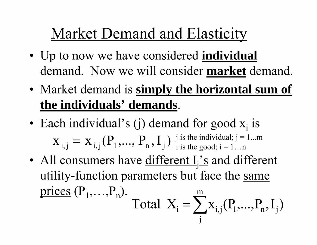
• Up to now we have considered individualdemand. Now we will consider market demand.

• Market demand is simply the horizontal sum of the individuals’ demands.

• Each individual’s (j) demand for good xi is

• All consumers have different Ij’s and different utility-function parameters but face the same prices (P1,…,Pn).

)I,P,...,(Pxx jn1ji,ji,

Market Demand and Elasticity

m

jjn1ji,i )I,P,...,(PxXTotal

j is the individual; j = 1...mi is the good; i = 1…n

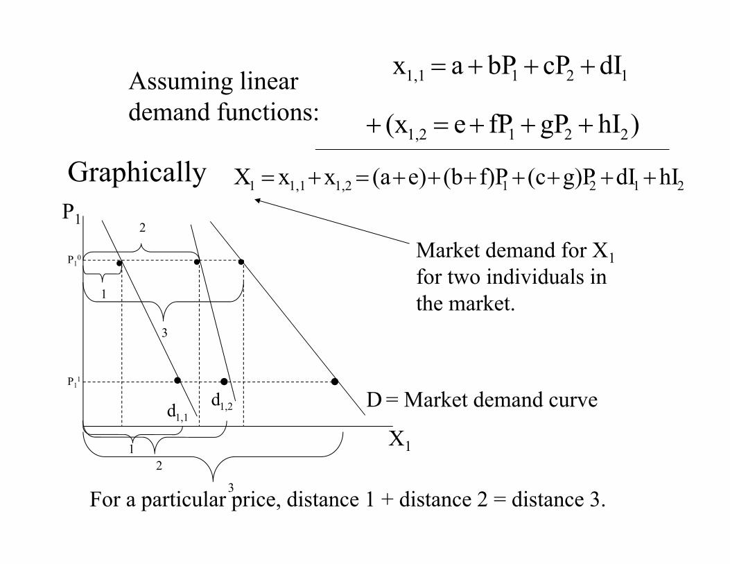
)hIgPfPe(x

dIcPbPax

2211,2

1211,1

21211,21,11 hIdIg)P(cf)P(be)(axxX

D = Market demand curve

P1

Market demand for X1for two individuals in the market.

Graphically

X1

1

2

3

1,1d 1,2d

For a particular price, distance 1 + distance 2 = distance 3.

2

3

1

Assuming linear demand functions:

P10

P11

• When individual demand curves shift, so does the market demand curve, although when only one individual’s demand curve shifts, market demand may not shift perceptibly.

• Sometimes movements are unambiguous because all individual demand curves move in the same direction.

• However, in other cases, movements in individual demands may be in different directions, because for different individuals a good may be normal or inferior and/or it may be a gross substitute or a gross complement for another good.

• Which way will D move? Existence of income effects and relationships between goods over many individuals may make market demand respond ambiguously.Preferences may also be different across individuals.

Own-Price Elasticity of Demand

goods.other of prices is P where,QP

PI),P(P,Qe

D

DPQ,

(-) (+)

eQ,P ≤ 0 except for Giffen good.

P,Q-space coordinate for where you are on the demand curve.

1e1e1e

P,Q

P,Q

P,Q Elastic

Unit elastic

InelasticMany economists think about elasticities in absolute value terms, so they reverse the operators (e.g., > becomes <), but we will view them as above.

Q

LARGE negative numbers less than -1 are elastic.P

P

Q

Q

SMALL negative numbers between -1 and 0 are inelastic.

P

Unit elastic.

Cross-Price Elasticity of Demand

QP

PQe PQ,

Gross Substitutes 0,e PQ, Gross Complements 0,e PQ, DQP

We don’t usually refer to cross-price elasticity as being “elastic” or “inelastic”.

DQP

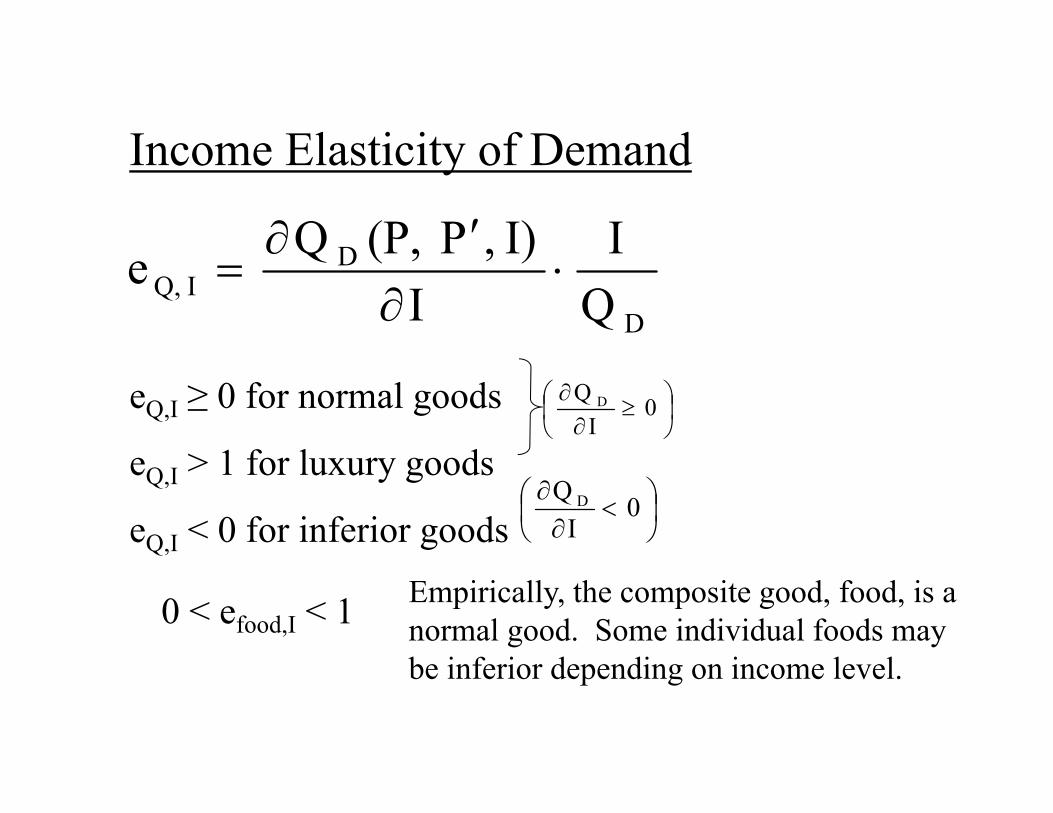
Income Elasticity of Demand

D

DIQ, Q

II

I),P(P,Qe

eQ,I ≥ 0 for normal goods

eQ,I > 1 for luxury goods

eQ,I < 0 for inferior goods

0

IQ D

0

IQ D

0 < efood,I < 1 Empirically, the composite good, food, is a normal good. Some individual foods may be inferior depending on income level.

• In price determination, we generally divide lengths of run into:– Very short run: Changes in quantity are not

possible.– Short run: Existing firms can change their

quantity by changing variable inputs, but firms will not enter or exit the industry, and at least one input is fixed (fixed costs).

– Long run: Firms may enter and exit the industry and all inputs are variable.

Very Short-Run Pricing• Market period – Firms cannot change the quantities they

produce. The good is already produced and in the market place, and cannot be stored. For example, fresh fish or strawberries must be sold soon after harvest.

• Price simply rations the quantity supplied among consumers.• Price will adjust to clear the market.

QQDQS

P P S

QQ1,2,3

P3P2P1

D3D2

D1D1

S

We will assume a Perfectly Competitive Industry (Pure Competition). The assumptions are:– A large number of small firms exist in the industry, each

producing the same homogeneous product with the same technology and costs,

– Each firm attempts to maximize profit,– Each firm is a price taker: It assumes that its actions

have no effect on market price.– Information is perfect: Prices are assumed to be known

by all market participants, – Transactions are costless: Buyers and sellers incur no

costs in making exchanges.Are these assumptions realistic? Why do we make

these assumptions?

Short-Run Pricing

• Each firm in the industry has a supply curve as shown in the last chapter; q depends on P, v, and w (v and w are fixed, while q varies with P).

• The number of firms is fixed.• q produced by each firm is variable. They can change q by

changing the variable input levels.• They cannot change the fixed inputs.• Market supply curve is the horizontal sum of the SMC

curves of all firms in the industry.

Firm 1 Firm 2 Firm 3 Industry

P

q

SMC1S

QS

P

w).v,(P,qw)v,(P,Qn

1iiS

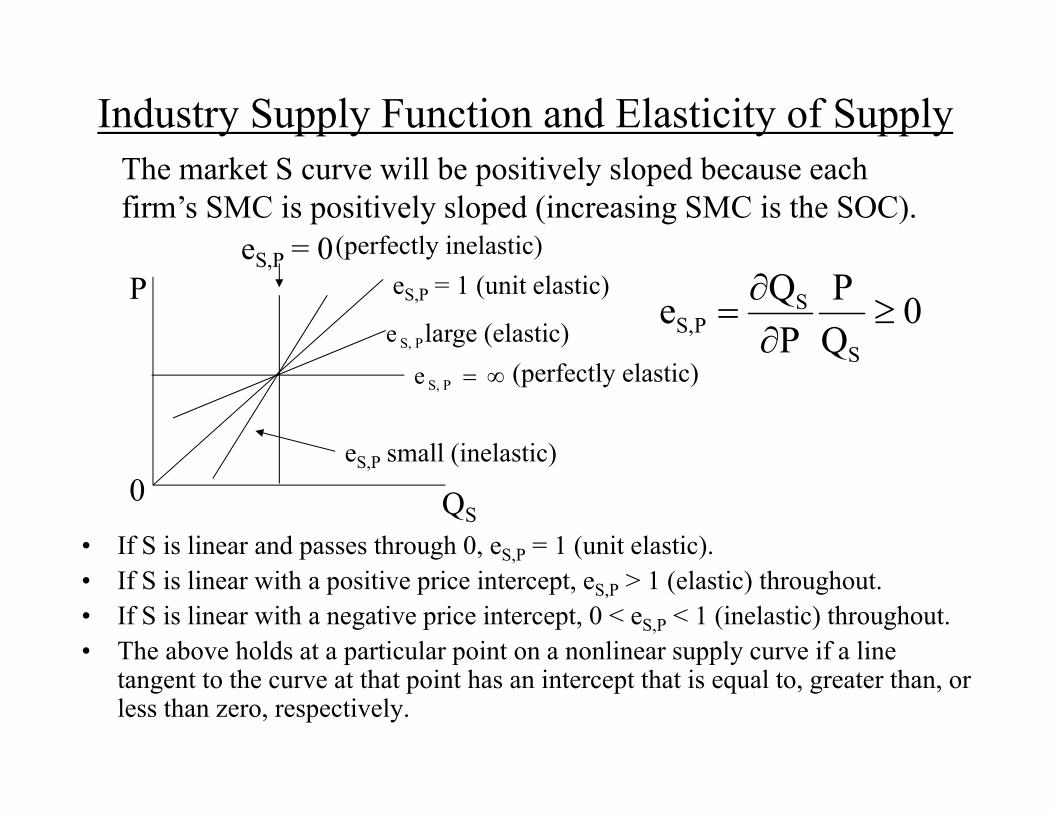
Industry Supply Function and Elasticity of Supply

• If S is linear and passes through 0, eS,P = 1 (unit elastic).• If S is linear with a positive price intercept, eS,P > 1 (elastic) throughout.• If S is linear with a negative price intercept, 0 < eS,P < 1 (inelastic) throughout.• The above holds at a particular point on a nonlinear supply curve if a line

tangent to the curve at that point has an intercept that is equal to, greater than, or less than zero, respectively.

0QP

PQe

S

SPS,

P

0

eS,P = 0

QS

eS,P = 1 (unit elastic)

PS,ePS,e large (elastic)

eS,P small (inelastic)

(perfectly elastic)

(perfectly inelastic)

The market S curve will be positively sloped because each firm’s SMC is positively sloped (increasing SMC is the SOC).

Market supply and demand curves interact to determine the market price (P).

q

SMC changes for only one firm

d changes for only one consumer

P

P1

0

SMC'SMC

SAC

qq1

P dD SMCS

0 Q1 = QS = QDQ

P

01q 1q

d1

All firms and consumers (market)

Solve S and D simultaneously

1d

1q

Trace logical sequence for constructing graphs: 1) Individual d curve, 2) , 3) Firm’s SMC, 4) SMC = S, 5) Solve S and D simultaneously to determine P1, 6) At P1, q1 is produced by firm, 7) At P1, is consumed by individual, and 8) and π > 0 can occur in the short run.

i

Dd

F

1q.qQQQq

i1D1S

F1

P1 is the equilibrium between the costs of firms and the demands (preferences) of individuals. Price acts as a signal to producers, and price acts as a signal to consumers.The equilibrium price is the price where QD = QS. Both suppliers and demanders are doing as they wish,

given the conditions (prices, costs, income, preferences, and technology).Suppose the individual (only one) has an increase in d. Market P and Q will change by only an

imperceptible amount because D will not change significantly.Suppose the firm (only one) has an increase in SMC. Market P and Q will change by only an

imperceptible amount because S will not change significantly (SAC' is not shown in graph).Price does not change when demand for one consumer changes or short-run marginal cost for one

firm changes because each firm and consumer account for only a very small amount of the market (see assumptions). Only quantity produced or consumed for the one firm or consumer changes.

w)v,,(PQI),P,(PQ 1S1D

Suppose demands for many individuals change:

Firm Market Individual

P

P2

0

SMCSAC

qq2q1

P

0 Q2Q

P

01q 2q

One of manyOne of many

All firms and individuals in the

P1

Q1

D D'

S

3q

A new short-run equilibrium is established because Market D increases to D'. S does not shift because in the short run the number of firms in the industry does not increase.

dd

q

Demand changes for many

π > 0 can occur in the short run.

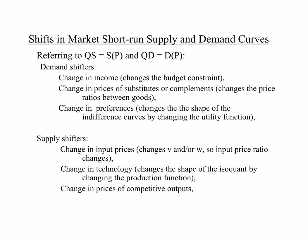
Shifts in Market Short-run Supply and Demand CurvesReferring to QS = S(P) and QD = D(P):Demand shifters:

Change in income (changes the budget constraint),Change in prices of substitutes or complements (changes the price

ratios between goods), Change in preferences (changes the the shape of the

indifference curves by changing the utility function),

Supply shifters:Change in input prices (changes v and/or w, so input price ratio

changes),Change in technology (changes the shape of the isoquant by

changing the production function),Change in prices of competitive outputs,

With elastic D, a change in S has little effect on P but a large effect on Q.

With inelastic D*, a change in S has a large effect on P but little effect on Q.

With an inelastic D curve (D*), changes in costs change P a lot, but result in only small changes in Q. U.S. agriculture is in this situation. Decreases in costs of production (SMC) cause relatively large decreases in output prices as supply increases.

Could also look at the effects of the elasticity of supply on P and Q caused by shifts in D. In agriculture, supply is inelastic, so changes in demand cause relatively large changes in price. In the U.S., changes in D are relatively minor compared with changes in S.

SS

PP

*P*QQ Q

*D

D

Effects of shifts in S or D depend on shape of the other curve (mostly slope).

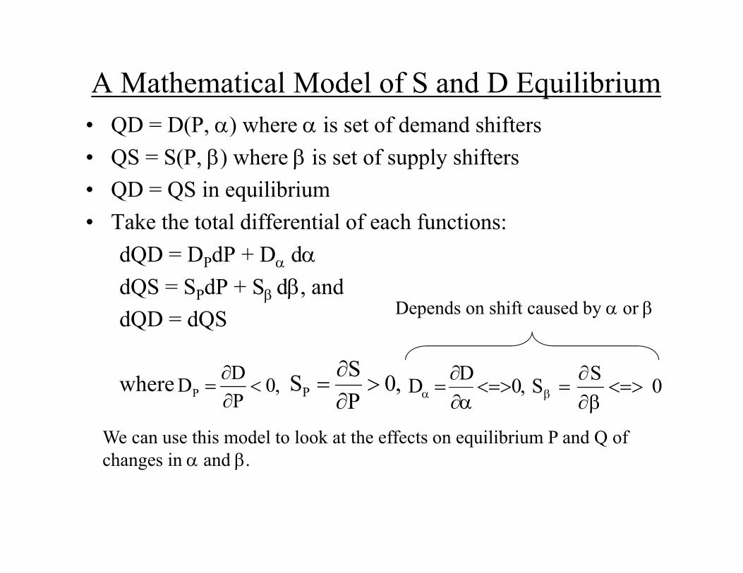
A Mathematical Model of S and D Equilibrium• QD = D(P, ) where is set of demand shifters• QS = S(P, ) where is set of supply shifters• QD = QS in equilibrium• Take the total differential of each functions:

dQD = DPdP + D ddQS = SPdP + S d, anddQD = dQS

where ,0PDDP

,0PSSP

,0DD

0SS

Depends on shift caused by or

We can use this model to look at the effects on equilibrium P and Q of changes in and .

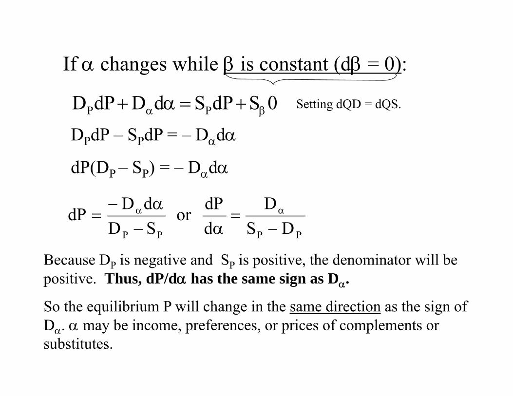
If changes while is constant (d = 0):

0SdPSdDdPD PP

DPdP – SPdP = – Dd

dP(DP – SP) = – Dd

PPPP DSD

ddPor

SDdDdP

Setting dQD = dQS.

Because DP is negative and SP is positive, the denominator will be positive. Thus, dP/d has the same sign as D.

So the equilibrium P will change in the same direction as the sign of D. may be income, preferences, or prices of complements or substitutes.

• If d = 0 and d 0, then Dd = 0, so

DPdP – SPdP = Sd

dP(DP – SP) = Sd

dβS

)S(DdPβ

PP

PP SDS

ddPor

Because DP is negative and SP is positive, the denominator will be negative. Thus, dP/d has the opposite sign as S.

So the equilibrium P will change in the opposite direction as the sign of S. may be the price of an input, technology, or the price of a competing product.

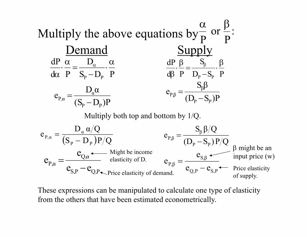
Multiply the above equations byDemand Supply

:P

orP

PDSD

PddP

PP

PSDS

PddP

PP

)PD(SαDe

PP

αP,α

QPDSQαDe

PP

αP,α

PQ,PS,

Q,αP,α ee

ee

Might be income elasticity of D.

PS,PQ,

βS,βP, ee

ee

might be an input price (w)

Multiply both top and bottom by 1/Q.

)PS(DβS

ePP

ββP,

QP)S(DQβS

ePP

ββP,

Price elasticity of demand.Price elasticity of supply.

These expressions can be manipulated to calculate one type of elasticity from the others that have been estimated econometrically.

Long-Run Pricing in Pure Competition

• In the long run, all inputs are variable and firms may enter and exit the industry.

• Each firm will operate at its most efficient plant size (SAC) at the low point on its AC curve.

• Long-run cost curves are used for decision-making.

q1

$

P1

0

SMC

MC

SAC

AC

q

d = AR = MR =

INDUSTRY

P = MC criterion

$

0Q1

SS = SMC

QQ1 = nq1, where n = number of firms in the industry.

P1

ONE OF MANY FIRMS

In the long run, there are no fixed costs. Any price below P1 will cause exits from the industry because firms earn an economic loss and any price above P1 will cause entries into the industry because firms earn an economic profit. These graphs depict long-run equilibrium where P=MR=AR=d=SMC=MC =Min SAC=Min AC

D= di

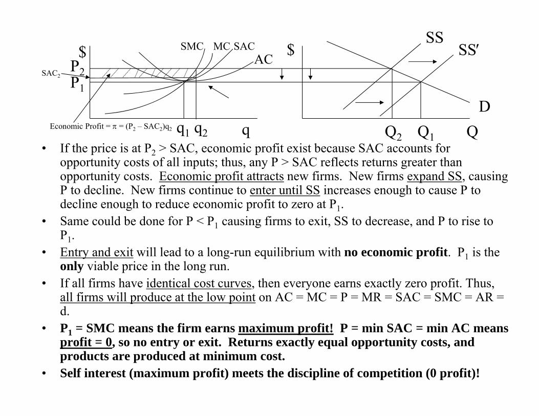
• If the price is at P2 > SAC, economic profit exist because SAC accounts for opportunity costs of all inputs; thus, any P > SAC reflects returns greater than opportunity costs. Economic profit attracts new firms. New firms expand SS, causing P to decline. New firms continue to enter until SS increases enough to cause P to decline enough to reduce economic profit to zero at P1.

• Same could be done for P < P1 causing firms to exit, SS to decrease, and P to rise to P1.

• Entry and exit will lead to a long-run equilibrium with no economic profit. P1 is the only viable price in the long run.

• If all firms have identical cost curves, then everyone earns exactly zero profit. Thus, all firms will produce at the low point on AC = MC = P = MR = SAC = SMC = AR = d.

• P1 = SMC means the firm earns maximum profit! P = min SAC = min AC means profit = 0, so no entry or exit. Returns exactly equal opportunity costs, and products are produced at minimum cost.

• Self interest (maximum profit) meets the discipline of competition (0 profit)!

SS

Economic Profit = = (P2 – SAC2)q2

$

P1

P2

q1 q2 q

SMC MC SACAC $ SS

DQ2 Q1 Q

SAC2

Constant, Increasing, and Decreasing Cost Industries

1. Constant Cost – Entry or exit of firms does not affectinput costs.

2. Increasing Cost – Entry (or exit) increases (or decreases) input costs.

3. Decreasing Cost – Entry (or exit) decreases (or increases) input costs.

In the long run, the MC curve does not relate specifically to the long-run supply curve as in the case of short-run supply relating to the SMC curve. Rather, it is the MC = MR = P intersection at minimum AC that shows how Q responds to P. The emphasis is on minimum AC.

P3 P1

q1 q2 Q2 Q3 Qq3Q1

LRS

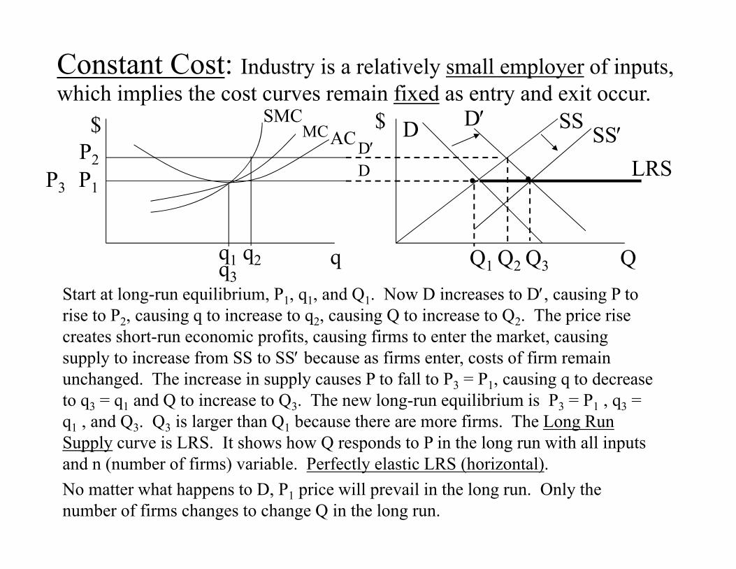
Start at long-run equilibrium, P1, q1, and Q1. Now D increases to D, causing P to rise to P2, causing q to increase to q2, causing Q to increase to Q2. The price rise creates short-run economic profits, causing firms to enter the market, causing supply to increase from SS to SS because as firms enter, costs of firm remain unchanged. The increase in supply causes P to fall to P3 = P1, causing q to decrease to q3 = q1 and Q to increase to Q3. The new long-run equilibrium is P3 = P1 , q3 = q1 , and Q3. Q3 is larger than Q1 because there are more firms. The Long Run Supply curve is LRS. It shows how Q responds to P in the long run with all inputs and n (number of firms) variable. Perfectly elastic LRS (horizontal).No matter what happens to D, P1 price will prevail in the long run. Only the number of firms changes to change Q in the long run.

$P2

q

SMCAC

$MCDD

SS SSDD

Constant Cost: Industry is a relatively small employer of inputs, which implies the cost curves remain fixed as entry and exit occur.

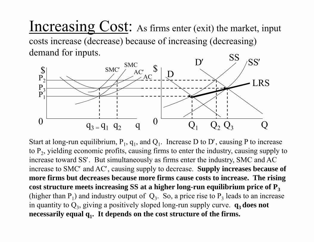
Increasing Cost: As firms enter (exit) the market, input costs increase (decrease) because of increasing (decreasing) demand for inputs.

$

q

$

0 0q2q3 = q1 QQ1 Q2 Q3

LRS

DD SS SS

ACACSMC

SMC

P2P3P1

Start at long-run equilibrium, P1, q1, and Q1. Increase D to D, causing P to increase to P2, yielding economic profits, causing firms to enter the industry, causing supply to increase toward SS. But simultaneously as firms enter the industry, SMC and AC increase to SMC and AC, causing supply to decrease. Supply increases because of more firms but decreases because more firms cause costs to increase. The rising cost structure meets increasing SS at a higher long-run equilibrium price of P3(higher than P1) and industry output of Q3. So, a price rise to P3 leads to an increase in quantity to Q3, giving a positively sloped long-run supply curve. q3 does not necessarily equal q1. It depends on the cost structure of the firms.

Decreasing Cost: Decreasing costs may result from a larger pool of trained labor, better infrastructure, economies of size among input suppliers as the industry grows larger (n increases) (eg., the computer industry).

$

q

$

0 0q2q1 QQ1 Q2 Q3

P2

P1

SMC SMC1

AC1

AC

q3

D D1SS

SS

LRSP3

Start at long-run equilibrium, P1, q1, and Q1. Increase D to D1, causing P to increase to P2, yielding economic profits, causing firms to enter the industry, causing supply to increase toward SS. But simultaneously as firms enter the industry, SMC and AC decrease to SMC1 and AC1, causing supply to increase even further. Supply increases because of more firms and increases because more firms cause costs to decrease. The declining cost structure is overtaken by increasing SS at a lower long-run equilibrium price of P3 (lower than P1) and industry output of Q3. So, a price fall to P3 leads to an increase in quantity to Q3, giving a negatively sloped long-run supply curve. With the cost structure graphed here, q3 does not equal q1, but they could be equal. It depends on the cost structure of the firms.

Long-Run Supply Elasticity• The LRS curve incorporates all adjustments that occur within the firm

and in the industry outside the firm (eg., changing cost structure).

• eLS,P may be negative (decreasing cost) as well as positive (increasing cost) or infinity (constant cost). LRS will be more elastic than SS.

P%Q%

QP

PQe PLS,

Q is a long-run adjustment to P.

eLS,P > 0

LRS

P,LSe0e P,LS

Q

P Changes in the number of firmsA new equilibrium implies a change in the number of firms in the industry.If Q0 is initial industry equilibrium output and q0

* is the optimal firm output, then the number of firms in the industry is .qQn *

000

If the D causes Q to rise to Q1, then and the change in n is In the constant cost industry case,

so n is a function of Q only.

*111 qQn

.qQqQnnn *00

*1101 ,

qQQnso,qq *

0

01*0

*1

In the increasing and decreasing cost industry cases, may not equal , implying a change in optimal firm size.

*1q

We could do the same for a decreasing cost industry for a decrease in cost as the initial stimulus; just switch q1

* and q0* around on the

graph. Even for a constant cost industry, changes in input costs (as the initial stimulus) may obviously result in a different q* at the new equilibrium Q.

Eg., With an increase in D for an increasing cost industry or increase in input cost as initial stimulus, could have either of the following.

*0q *

1q *1q *

0q

AC2AC1

AC2AC1P

*0q

Producer Surplus in Long Run, Ricardian Rent, and Capitalization of Rents

Producer surplus is the extra return producers make by making transactions at the market price over and above what they would earn if nothing were produced. Graphically it is similar to short-run producer surplus; the area above the long-run supply curve below the market price.

In the long run, profits are zero at the market price, so who receives the gain? Producer surplus goes to the owners of the inputs in the form of higher input prices.

For a constant-cost industry, returns to inputs are independent of the level of output; producer surplus is zero.

For an increasing-cost industry, input prices are bid up as output increases, so returns to inputs increase; producer surplus is positive. Input prices must increase to attract more and more highly productive resources to the industry. Vice versa for decreasing-cost industry.

Ricardian rents are profits earned by firms (low cost firms) with resources that are more productive than needed to earn zero profit at the market price (eg., crop land). These profits can persist in the long run.

Capitalization of rents simply means that input prices increase to reflect the present value of future profits earned by the input (eg., more productive land earns higher profits, so land price will be higher for more productive land than for less productive land). Therefore, future profits are said to be capitalized into the price of input. Producer surplus goes to owners of the inputs that cause an upward sloping long-run industry supply curve.