chapter 10 segmentation - utrecht university · · 2005-11-09chapter 10 segmentation t he...
TRANSCRIPT

Chapter 10
Segmentation
The division of an image into meaningful structures, image segmentation, is often anessential step in image analysis, object representation, visualization, and manyother image processing tasks. In chapter 8, we focussed on how to analyze and
represent an object, but we assumed the group of pixels that identified that object wasknown beforehand. In this chapter, we will focus on methods that find the particularpixels that make up an object.
A great variety of segmentation methods has been proposed in the past decades, andsome categorization is necessary to present the methods properly here. A disjunct cat-egorization does not seem to be possible though, because even two very different seg-mentation approaches may share properties that defy singular categorization1. The cat-egorization presented in this chapter is therefore rather a categorization regarding theemphasis of an approach than a strict division.
The following categories are used:
• Threshold based segmentation. Histogram thresholding and slicing techniquesare used to segment the image. They may be applied directly to an image, but canalso be combined with pre- and post-processing techniques.• Edge based segmentation. With this technique, detected edges in an image are
assumed to represent object boundaries, and used to identify these objects.• Region based segmentation. Where an edge based technique may attempt to find
the object boundaries and then locate the object itself by filling them in, a regionbased technique takes the opposite approach, by (e.g.) starting in the middle of anobject and then “growing” outward until it meets the object boundaries.
1In much the same way as the platypus does not seem to fit in any of normal zoological categories. Itseems that any segmentation method categorized as a mammal, upon closer inspection, appears to havesome aspect that shows it to be laying eggs.
274 Segmentation
• Clustering techniques. Although clustering is sometimes used as a synonym for(agglomerative) segmentation techniques, we use it here to denote techniques thatare primarily used in exploratory data analysis of high-dimensional measurementpatterns. In this context, clustering methods attempt to group together patternsthat are similar in some sense. This goal is very similar to what we are attemptingto do when we segment an image, and indeed some clustering techniques canreadily be applied for image segmentation.• Matching. When we know what an object we wish to identify in an image (ap-
proximately) looks like, we can use this knowledge to locate the object in an image.This approach to segmentation is called matching.
Perfect image segmentation –i.e., each pixel is assigned to the correct object segment–is a goal that cannot usually be achieved. Indeed, because of the way a digital imageis acquired, this may be impossible, since a pixel may straddle the “real” boundaryof objects such that it partially belongs to two (or even more) objects. Most methodspresented here –indeed most current segmentation methods– only attempt to assign apixel to a single segment, which is an approach that is more than adequate for mostapplications. Methods that assign a segment probability distribution to each pixel arecalled probabilistic. This class of methods is theoretically more accurate, and applicationswhere a probabilistic approach is the only approach accurate enough for specific objectmeasurements can easily be named. However, probabilistic techniques add consider-able complexity to segmentation –both in the sense of concept and implementation–and as such are still little used.
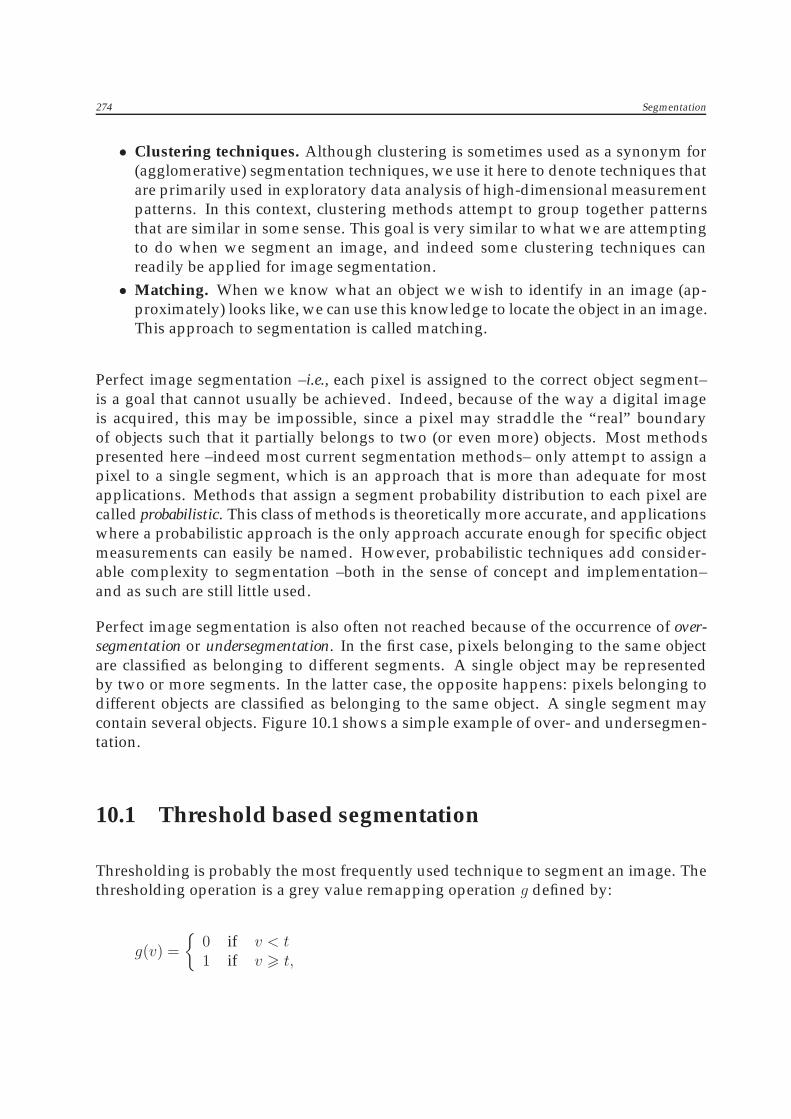
Perfect image segmentation is also often not reached because of the occurrence of over-segmentation or undersegmentation. In the first case, pixels belonging to the same objectare classified as belonging to different segments. A single object may be representedby two or more segments. In the latter case, the opposite happens: pixels belonging todifferent objects are classified as belonging to the same object. A single segment maycontain several objects. Figure 10.1 shows a simple example of over- and undersegmen-tation.
10.1 Threshold based segmentation
Thresholding is probably the most frequently used technique to segment an image. Thethresholding operation is a grey value remapping operation g defined by:
g(v) =
{0 if v < t1 if v � t,
10.1 Threshold based segmentation 275
Figure 10.1 An original image is shown at the top left. If it is known that this image containsonly uniformly sized squares, then the image on the top right shows the correct segmentation.Each segment has been indicated by a unique grey value here. The bottom left and right imagesshow examples of oversegmentation and undersegmentation respectively.
where v represents a grey value, and t is the threshold value. Thresholding maps agrey-valued image to a binary image. After the thresholding operation, the image hasbeen segmented into two segments, identified by the pixel values 0 and 1 respectively.
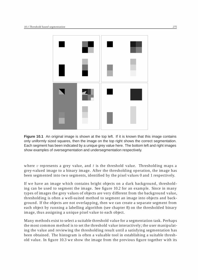
If we have an image which contains bright objects on a dark background, threshold-ing can be used to segment the image. See figure 10.2 for an example. Since in manytypes of images the grey values of objects are very different from the background value,thresholding is often a well-suited method to segment an image into objects and back-ground. If the objects are not overlapping, then we can create a separate segment fromeach object by running a labelling algorithm (see chapter 8) on the thresholded binaryimage, thus assigning a unique pixel value to each object.
Many methods exist to select a suitable threshold value for a segmentation task. Perhapsthe most common method is to set the threshold value interactively; the user manipulat-ing the value and reviewing the thresholding result until a satisfying segmentation hasbeen obtained. The histogram is often a valuable tool in establishing a suitable thresh-old value. In figure 10.3 we show the image from the previous figure together with its
276 Segmentation
Figure 10.2 Example of segmentation by thresholding. On the left, an original image withbright objects (the pencils) on a dark background. Thresholding using an appropriate thresholdsegments the image into objects (segment with value 1) and background (segment with value0).
histogram, and the thresholding results using four different threshold values obtainedfrom the histogram. In the next section, threshold selection methods are discussed inmore detail.
When several desired segments in an image can be distinguished by their grey values,threshold segmentation can be extended to use multiple thresholds to segment an imageinto more than two segments: all pixels with a value smaller than the first threshold areassigned to segment 0, all pixels with values between the first and second threshold areassigned to segment 1, all pixels with values between the second and third thresholdare assigned to segment 2, etc. If n thresholds (t1, t2, . . . , tn) are used:
g(v) =
⎧⎪⎪⎪⎪⎪⎨⎪⎪⎪⎪⎪⎩
0 if v < t11 if t1 � v < t22 if t2 � v < t3...
......
n if tn � v.
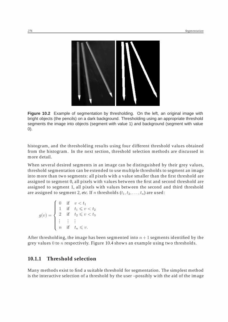
After thresholding, the image has been segmented into n+ 1 segments identified by thegrey values 0 to n respectively. Figure 10.4 shows an example using two thresholds.
10.1.1 Threshold selection
Many methods exist to find a suitable threshold for segmentation. The simplest methodis the interactive selection of a threshold by the user –possibly with the aid of the image

10.1 Threshold based segmentation 277
Freq
uenc
y
Grey value
Thr 1 Thr 2 Thr 3 Thr 4
Figure 10.3 Example of threshold selection from the histogram. Top row: original image andhistogram. Four special grey values (indicated by Thr 1,2,3,4) have been chosen. The bottomrow shows the respective thresholding results at each of the values. At a first glance, the originalimage appears to have only three grey values. But the histogram shows that the grey valuedistribution is more diffuse; that the three basic values are in fact spread out over a certainrange. Because the background grey values occur most frequently, we expect all of the largevalues in the left part of the histogram to correspond to the background. This is indeed the case.The result of threshold 1 shows that the peak between thresholds 1 and 2 also corresponds tobackground values. The result of threshold 2 shows the desired segmentation; every grey valueto the right of threshold 2 corresponds to the pencils. Threshold 4 shows that the right-most littlepeak corresponds to the bright grey value in the tips of the pencils.
278 Segmentation
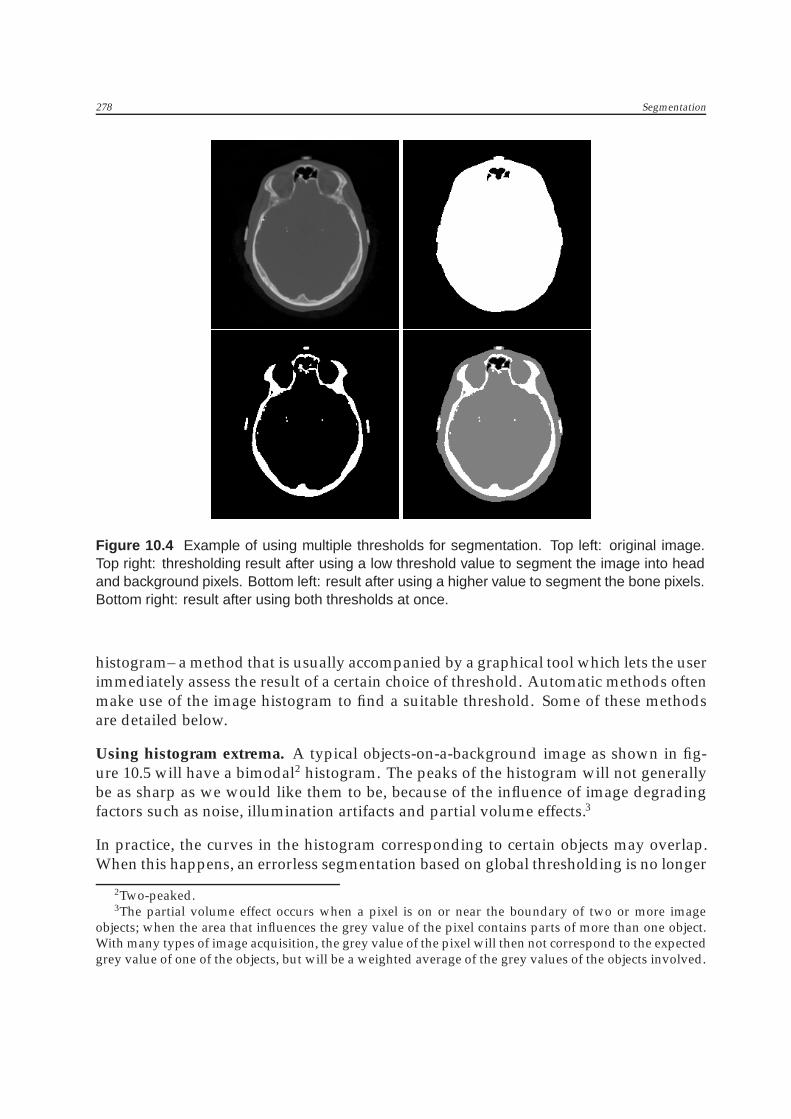
Figure 10.4 Example of using multiple thresholds for segmentation. Top left: original image.Top right: thresholding result after using a low threshold value to segment the image into headand background pixels. Bottom left: result after using a higher value to segment the bone pixels.Bottom right: result after using both thresholds at once.
histogram– a method that is usually accompanied by a graphical tool which lets the userimmediately assess the result of a certain choice of threshold. Automatic methods oftenmake use of the image histogram to find a suitable threshold. Some of these methodsare detailed below.
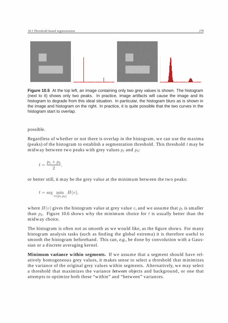
Using histogram extrema. A typical objects-on-a-background image as shown in fig-ure 10.5 will have a bimodal2 histogram. The peaks of the histogram will not generallybe as sharp as we would like them to be, because of the influence of image degradingfactors such as noise, illumination artifacts and partial volume effects.3
In practice, the curves in the histogram corresponding to certain objects may overlap.When this happens, an errorless segmentation based on global thresholding is no longer
2Two-peaked.3The partial volume effect occurs when a pixel is on or near the boundary of two or more image
objects; when the area that influences the grey value of the pixel contains parts of more than one object.With many types of image acquisition, the grey value of the pixel will then not correspond to the expectedgrey value of one of the objects, but will be a weighted average of the grey values of the objects involved.
10.1 Threshold based segmentation 279
Figure 10.5 At the top left, an image containing only two grey values is shown. The histogram(next to it) shows only two peaks. In practice, image artifacts will cause the image and itshistogram to degrade from this ideal situation. In particular, the histogram blurs as is shown inthe image and histogram on the right. In practice, it is quite possible that the two curves in thehistogram start to overlap.
possible.
Regardless of whether or not there is overlap in the histogram, we can use the maxima(peaks) of the histogram to establish a segmentation threshold. This threshold t may bemidway between two peaks with grey values p1 and p2:
t =p1 + p2
2,
or better still, it may be the grey value at the minimum between the two peaks:
t = arg minv∈[p1,p2]
H(v),
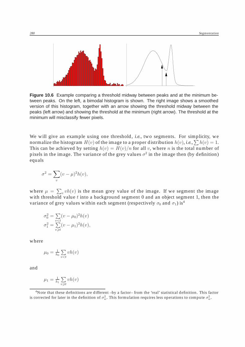
where H(v) gives the histogram value at grey value v, and we assume that p1 is smallerthan p2. Figure 10.6 shows why the minimum choice for t is usually better than themidway choice.
The histogram is often not as smooth as we would like, as the figure shows. For manyhistogram analysis tasks (such as finding the global extrema) it is therefore useful tosmooth the histogram beforehand. This can, e.g., be done by convolution with a Gaus-sian or a discrete averaging kernel.
Minimum variance within segments. If we assume that a segment should have rel-atively homogeneous grey values, it makes sense to select a threshold that minimizesthe variance of the original grey values within segments. Alternatively, we may selecta threshold that maximizes the variance between objects and background, or one thatattempts to optimize both these “within” and “between” variances.
280 Segmentation
Figure 10.6 Example comparing a threshold midway between peaks and at the minimum be-tween peaks. On the left, a bimodal histogram is shown. The right image shows a smoothedversion of this histogram, together with an arrow showing the threshold midway between thepeaks (left arrow) and showing the threshold at the minimum (right arrow). The threshold at theminimum will misclassify fewer pixels.
We will give an example using one threshold, i.e., two segments. For simplicity, wenormalize the histogramH(v) of the image to a proper distribution h(v), i.e.,
∑h(v) = 1.
This can be achieved by setting h(v) = H(v)/n for all v, where n is the total number ofpixels in the image. The variance of the grey values σ2 in the image then (by definition)equals
σ2 =∑v
(v − μ)2h(v),
where μ =∑
v vh(v) is the mean grey value of the image. If we segment the imagewith threshold value t into a background segment 0 and an object segment 1, then thevariance of grey values within each segment (respectively σ0 and σ1) is4
σ20 =
∑v<t
(v − μ0)2h(v)
σ21 =
∑v�t
(v − μ1)2h(v),
where
μ0 = 1h0
∑v<t
vh(v)
and
μ1 = 1h1
∑v�t
vh(v)
4Note that these definitions are different –by a factor– from the ‘real’ statistical definition. This factoris corrected for later in the definition of σ2
w. This formulation requires less operations to compute σ2w.

10.1 Threshold based segmentation 281
are the mean grey values of the respective segments 0 and 1. The probabilities h0 and h1
that a randomly selected pixel belongs to segment 0 or 1 are
h0 =∑v<t
h(v)
h1 =∑v�t
h(v).
Note that h0 + h1 = 1. The total variance within segments σ2w is
σ2w = h0σ
20 + h1σ
21.
This variance only depends on the threshold value t: σ2w = σ2
w(t). This means that we canfind the value of t that minimizes the variance within segments by minimizing σ2
w(t).
The variance between the segments 0 and 1, σ2b , is
σ2b = h0(μ0 − μ)2 + h1(μ1 − μ)2.
Again, this variance is only dependent on the threshold value t. Finding the t that max-imizes σ2
b maximizes the variance between segments. A hybrid approach that attemptsto maximize σ2
b while minimizing σ2w is to find the threshold t that maximizes the ratio
σ2b/σ
2w.
If more than two segments are required, the method described above can be extendedto use multiple thresholds. The variances σ2
w and σ2b will then be functions of more than
one threshold, so we need multi-dimensional optimization to find the set of optimalthresholds. Since this is especially cumbersome if the number of segments is large, amore practical algorithm that minimizes the variances within segments is often used,an iterative algorithm known as K-means clustering.
Algorithm: K-means clusteringThe objective of theK-means clustering algorithm is to divide an image intoK segments(using K − 1 thresholds), minimizing the total within-segment variance. The variable Kmust be set before running the algorithm.
The within-segment variance σ2w is defined by
σ2w =
K−1∑i=0
hiσ2i ,
where hi =∑
v∈Sih(v) is the probability that a random pixel belongs to segment i (con-
taining the grey values in the range Si), σ2i =
∑v∈Si
(v − μi)2h(v) is the variance of greyvalues of segment i, and μi =
∑v∈Si
vh(v) is the mean grey value in segment i. Alldefinitions are as before in the case with a single threshold.
282 Segmentation
1. Initialization: distribute the K − 1 thresholds over the histogram. (For example insuch a way that the grey value range is divided into K pieces of equal length.)Segment the image according to the thresholds set. For each segment, computethe ’cluster center’,i.e., the value midway between the two thresholds that makeup the segment.
2. For each segment, compute the mean pixel value μi.
3. Reset the cluster centers to the computed values μi.
4. Reset the thresholds to be midway between the cluster centers, and segment theimage.
5. Go to step 2. Iterate until the cluster centers do not move anymore (or do not movesignificantly).
Note that this algorithm –although it minimizes a variance– does not require any vari-ance to be computed explicitly!
The version of this algorithm with only one threshold (two segments) can be extractedfrom the general form above. In practice, the initialization step in this case is oftenslightly different to try to get the initial threshold close to the optimal position, so thealgorithm will converge faster. A heuristic rule is often used to achieve this. The algo-rithm –with a widely employed heuristic– then becomes:
Algorithm: Iterative thresholding
1. Assume that the four corner points of the image are background pixels (part ofsegment 0), and set μ0 to the average grey value of these four pixels. Assume allof the other pixels are object pixels, and set μ1 to their average grey value.
2. Set the threshold t to t = 12(μ0 + μ1), and segment the image.
3. Recompute μ0 and μ1, the mean of the original grey values of the two segments.
4. Go to step 2 and iterate until the threshold value no longer changes (or no longerchanges significantly).
Example
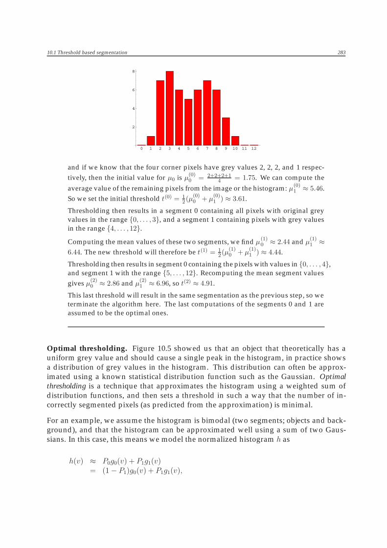
If we have an image with the following histogram:
10.1 Threshold based segmentation 283
0 1 2 3 4 5 6 7 8 9 10 11 12
2
4
6
8
and if we know that the four corner pixels have grey values 2, 2, 2, and 1 respec-tively, then the initial value for μ0 is μ(0)
0 = 2+2+2+14 = 1.75. We can compute the
average value of the remaining pixels from the image or the histogram: μ(0)1 ≈ 5.46.
So we set the initial threshold t(0) = 12 (μ(0)
0 + μ(0)1 ) ≈ 3.61.
Thresholding then results in a segment 0 containing all pixels with original greyvalues in the range {0, . . . , 3}, and a segment 1 containing pixels with grey valuesin the range {4, . . . , 12}.Computing the mean values of these two segments, we find μ(1)
0 ≈ 2.44 and μ(1)1 ≈
6.44. The new threshold will therefore be t(1) = 12(μ(1)
0 + μ(1)1 ) ≈ 4.44.
Thresholding then results in segment 0 containing the pixels with values in {0, . . . , 4},and segment 1 with the range {5, . . . , 12}. Recomputing the mean segment valuesgives μ(2)
0 ≈ 2.86 and μ(2)1 ≈ 6.96, so t(2) ≈ 4.91.
This last threshold will result in the same segmentation as the previous step, so weterminate the algorithm here. The last computations of the segments 0 and 1 areassumed to be the optimal ones.
Optimal thresholding. Figure 10.5 showed us that an object that theoretically has auniform grey value and should cause a single peak in the histogram, in practice showsa distribution of grey values in the histogram. This distribution can often be approx-imated using a known statistical distribution function such as the Gaussian. Optimalthresholding is a technique that approximates the histogram using a weighted sum ofdistribution functions, and then sets a threshold in such a way that the number of in-correctly segmented pixels (as predicted from the approximation) is minimal.
For an example, we assume the histogram is bimodal (two segments; objects and back-ground), and that the histogram can be approximated well using a sum of two Gaus-sians. In this case, this means we model the normalized histogram h as
h(v) ≈ P0g0(v) + P1g1(v)= (1− P1)g0(v) + P1g1(v),
284 Segmentation
where g0 and g1 are Gaussian functions with unknown mean and variance, and P0 andP1 are the global probabilities –also unknown– that a pixel belongs to segment 0 or 1respectively. Note that P0 + P1 = 1. This leaves us with five unknowns –two means,two variances, and P1– to be estimated from the image histogram. Figure 10.7 shows anexample bimodal histogram and its approximation using two Gaussians. The estima-tion of the unknowns is usually done using a non-linear curve fitting technique whichminimizes the sum of squared distances (as a function of the unknowns) between thehistogram data and the fitted curve, i.e.,
minimize∑v
(h(v)−m(v))2,
where m(v) is the chosen model for the histogram, which has the unknowns for param-eters (here m(v) = P0g0(v) + P1g1(v)). The estimation of the (here) five unknowns cantherefore be formulated as the minimization of a function of five variables. How thisminimization is achieved is beyond the scope of this book, but techniques for this arefairly standard and can easily be found in mathematics literature.
Assuming we can estimate all of the unknowns, the optimal threshold t is the grey valuewhere the two Gaussian curves intersect:
(1− P1)g0(t) = P1g1(t).
Intermezzo∗
This last equation can be deduced as follows:
The normalized histogram is approximated by
h(v) ≈ (1− P1)g0(v) + P1g1(v),
with g0(v) the distribution of background pixels, and g1(v) the distribution of ob-ject pixels. P1 and (1 − P1) are the fractions of object and background pixels re-spectively. If we threshold the image at a certain threshold t, then the fraction ofbackground misclassified as object pixels is
(1− P1)
∞∫t
g0(v)dv.
The fraction of object pixels misclassified as background pixels is
P1
t∫−∞
g1(v)dv.

10.1 Threshold based segmentation 285
The total error fraction E(t) is the sum of these partial errors:
E(t) = (1− P1)
∞∫t
g0(v)dv + P1
t∫−∞
g1(v)dv.
The error E(t) is minimal when the derivative is zero:
E′(t) = 0(1− P1)(−)g0(t) + P1g1(t) = 0(1− P1)g0(t) = P1g1(t).
Figure 10.7 Example of optimal thresholding. Left: image histogram. Right: approximationof the histogram (thick curve) using two Gaussians (thin curves). The right arrow shows theoptimal threshold. For comparison, the left arrow shows the threshold value if we had used theminimum-between-peaks criterion.
Optimal thresholding may be extended to use multiple thresholds, i.e., the normalizedhistogram is approximated using a sum of more than two Gaussians:
h(v) ≈k−1∑i=0
Pigi(v),
where gi is a Gaussian, Pi the global probability of a pixel belonging to segment i, andk the number of Gaussians used to model the histogram. Since the addition of eachGaussian to the model adds three parameters to be estimated, using this model be-comes increasingly fickle for large k. Moreover, selecting an appropriate value for kcan be a difficult problem by itself. The model can also be extended using other distri-butions than the Gaussian. The choice of the distribution function should be based onknowledge of the image acquisition process, from which the correct choice can often bededuced.
286 Segmentation
Histogram estimation. The optimal thresholding method described above uses an es-timation of the histogram –actually, a smooth curve that best fits the measured imagehistogram– rather than the histogram itself. Some of the other threshold selection meth-ods described previously also benefit from using a smooth estimate instead of the rawhistogram data. For example, the methods that require finding the extrema of the his-togram curve may be better off using a smooth estimate, since this way the chance ofgetting stuck in a local optimum is decreased, and the process is less susceptible to noisein the raw histogram data.
Good estimation of the histogram often does not require that all of the available pixelinformation is used. Using a small fraction of the grey values is usually sufficient for agood estimate. For example, instead of using all of the pixels (and their grey values) inthe estimation process, we could randomly select 5% of the image pixels and use onlythose in the process. In practice –unless the noise is exceedingly large or the number ofpixels in the image very small– adding the remaining 95% will not significantly improvethe estimation.
The approach to estimation used in optimal thresholding is an example of a parametricapproach. In this type of approach, the histogram is modeled by a function with a fixednumber of parameters, and the function is fitted to the histogram by twiddling with theparameters. A non-parametric approach to histogram estimation is any approach thatdoes not require the computation or approximation of parameters. The most frequentlyused method in this category is called Parzen windowing.
Parzen windowing estimates the histogram by a sum of simple distribution functions.In contrast to parametric techniques, the number of distribution functions is large ratherthan small. In fact, one function may be used for each pixel that is employed in theestimation process. Each distribution function used is identical to all others, and anyparameters of the distribution function are fixed to identical values beforehand. Forexample, the estimate may be a sum of Gaussians, all with a mean of 0 and a varianceof 1. In general the Parzen windowing estimate p(v) of the normalized histogram canbe written as
p(v) =1
N
∑i
d(v − vi),
where N is the number of pixels from the original image used in the estimation, vi isthe grey value of a pixel, i ∈ {1, 2, . . . , N}, and d is a distribution function (kernel). TheN pixels are usually sampled randomly or equidistantly from the original image. Thekernel d is usually a Gaussian or a block or triangular function centered around zerowith unit area, but other functions may also be used. Figure 10.8 shows an example ofa Parzen histogram estimate using a Gaussian function for the kernel d.

10.1 Threshold based segmentation 287
Figure 10.8 Example of Parzen windowing to estimate the histogram. In this example, theGaussian function with zero mean and unit variance was chosen for the distribution kernel. Asmall fraction of the pixels was sampled randomly from the image, and a Gaussian placed a thecorresponding grey value in the histogram. Left: original image histogram. Middle: Gaussianfunctions of the sampled pixels. Right: normalized sum of the Gaussians in the middle figure;the Parzen windowing estimate of the histogram.
In practice, non-parametric approaches such as Parzen windowing are often more flex-ible than parametric ones, as well as less computationally expensive. The better flex-ibility stems from the fact that no strong assumptions are made on the shape of thehistogram, while parametric approaches effectively straitjacket the shape by assumingthe histogram to be shaped like –for instance– the sum of two Gaussians.
10.1.2 Enhancing threshold segmentation
The segmentation of an image by thresholding is totally insensitive to the spatial contextof a pixel. There are many cases conceivable where a human observer may decide onthe basis of spatial context that a pixel is not part of a segment, even though it satis-fies a threshold criterion. For example, noise in an image may cause many very smallsegments5 when thresholding, while in many applications it is known that such smallsegments cannot physically exist (see figure 10.9). Or: segment boundaries may ap-pear bumpy while we know them to be smooth. Or: thresholding shows two objectsconnected by a thin ‘bridge’, while we know them to be separate objects.
Many techniques exist that address such problems. These techniques can be dividedinto three categories: processing of the original image prior to segmentation, processingof the segmented result, or adaptation of the segmentation process. Often, a combina-tion of these techniques is used in a single application. In this section we will give someexamples of common approaches.
The next two examples show the use of non-linear filters such as a median filter andmorphological operators for removing (often noise related) small scale artifacts.
5Or, depending on the implementation, a single segment including many small disjunct fragments.
288 Segmentation
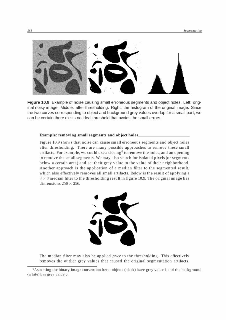
Figure 10.9 Example of noise causing small erroneous segments and object holes. Left: orig-inal noisy image. Middle: after thresholding. Right: the histogram of the original image. Sincethe two curves corresponding to object and background grey values overlap for a small part, wecan be certain there exists no ideal threshold that avoids the small errors.
Example: removing small segments and object holes
Figure 10.9 shows that noise can cause small erroneous segments and object holesafter thresholding. There are many possible approaches to remove these smallartifacts. For example, we could use a closing6 to remove the holes, and an openingto remove the small segments. We may also search for isolated pixels (or segmentsbelow a certain area) and set their grey value to the value of their neighborhood.Another approach is the application of a median filter to the segmented result,which also effectively removes all small artifacts. Below is the result of applying a3× 3 median filter to the thresholding result in figure 10.9. The original image hasdimensions 256 × 256.
The median filter may also be applied prior to the thresholding. This effectivelyremoves the outlier grey values that caused the original segmentation artifacts.
6Assuming the binary-image convention here: objects (black) have grey value 1 and the background(white) has grey value 0.

10.1 Threshold based segmentation 289
Below are the original image after application of a 3 × 3 median filter and thresh-olding:
Example: pre- and postprocessing using morphology
Consider these images:
The left image is a noisy original (256 × 256) image, the right image a binary im-age after thresholding the original. Needless to say, direct thresholding performspoorly on this type of original. The influence of noise can be reduced, however, bymaking the object in the original more coherent using a morphological operationsuch as closing. The left image below shows the original image after closing usinga 7× 7 square, the right image the result after thresholding this image:
290 Segmentation
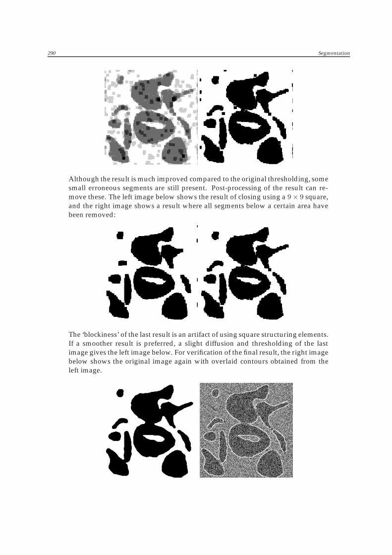
Although the result is much improved compared to the original thresholding, somesmall erroneous segments are still present. Post-processing of the result can re-move these. The left image below shows the result of closing using a 9× 9 square,and the right image shows a result where all segments below a certain area havebeen removed:
The ‘blockiness’ of the last result is an artifact of using square structuring elements.If a smoother result is preferred, a slight diffusion and thresholding of the lastimage gives the left image below. For verification of the final result, the right imagebelow shows the original image again with overlaid contours obtained from theleft image.
10.1 Threshold based segmentation 291
Large scale grey value artifacts, such as the occurrence of an illumination gradient acrossan image, can be handled in various ways. In chapter 6, we have already shown thatthe morphological white top hat transform (see figure 6.18) can be effective to removesuch a gradient. Fourier techniques are also often effective, because the gradient imageis a distinct low-frequency feature. A popular technique is the subtraction of a low-passfiltered image from an original image. Below are two examples showing yet other ap-proaches. The first is an adaptation of the thresholding algorithm that bases a thresholdon the local image grey values, i.e., based only on the neighborhood of a pixel ratherthan all of the grey values in an image. The second is a pre-processing technique thatestimates and removes the large grey value artifact from the image.
Example: local thresholding
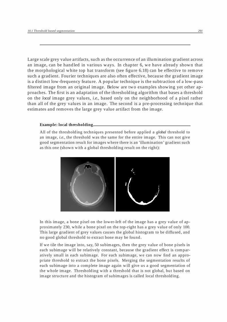
All of the thresholding techniques presented before applied a global threshold toan image, i.e., the threshold was the same for the entire image. This can not givegood segmentation result for images where there is an ’illumination’ gradient suchas this one (shown with a global thresholding result on the right):
In this image, a bone pixel on the lower-left of the image has a grey value of ap-proximately 230, while a bone pixel on the top-right has a grey value of only 100.This large gradient of grey values causes the global histogram to be diffused, andno good global threshold to extract bone may be found.
If we tile the image into, say, 50 subimages, then the grey value of bone pixels ineach subimage will be relatively constant, because the gradient effect is compar-atively small in each subimage. For each subimage, we can now find an appro-priate threshold to extract the bone pixels. Merging the segmentation results ofeach subimage into a complete image again will give us a good segmentation ofthe whole image. Thresholding with a threshold that is not global, but based onimage structure and the histogram of subimages is called local thresholding.
292 Segmentation
Local thresholding can be used effectively when the gradient effect is small withrespect to the chosen subimage size. If the gradient is too large, similar errors asin the global example will now occur within a subimage, and the segments foundwithin subimages will no longer match up adequately at the subimage seams. Thisis a telltale that the subimage size should be reduced. However, we cannot makethe subimage too small, because then a reliable histogram can no longer be made.
Example: using histogram entropy
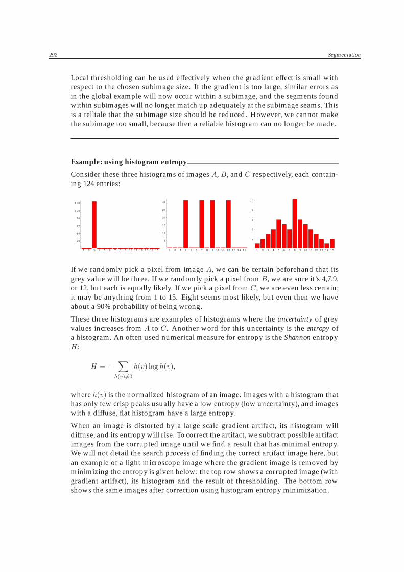
Consider these three histograms of images A, B, and C respectively, each contain-ing 124 entries:
1 2 3 4 5 6 7 8 9 10 11 12 13 14 15
20
40
60
80
100
120
1 2 3 4 5 6 7 8 9 10 11 12 13 14 15
5
10
15
20
25
30
1 2 3 4 5 6 7 8 9 10 11 12 13 14 15
2
4
6
8
10
If we randomly pick a pixel from image A, we can be certain beforehand that itsgrey value will be three. If we randomly pick a pixel from B, we are sure it’s 4,7,9,or 12, but each is equally likely. If we pick a pixel from C , we are even less certain;it may be anything from 1 to 15. Eight seems most likely, but even then we haveabout a 90% probability of being wrong.
These three histograms are examples of histograms where the uncertainty of greyvalues increases from A to C . Another word for this uncertainty is the entropy ofa histogram. An often used numerical measure for entropy is the Shannon entropyH :
H = −∑h(v)�=0
h(v) log h(v),
where h(v) is the normalized histogram of an image. Images with a histogram thathas only few crisp peaks usually have a low entropy (low uncertainty), and imageswith a diffuse, flat histogram have a large entropy.
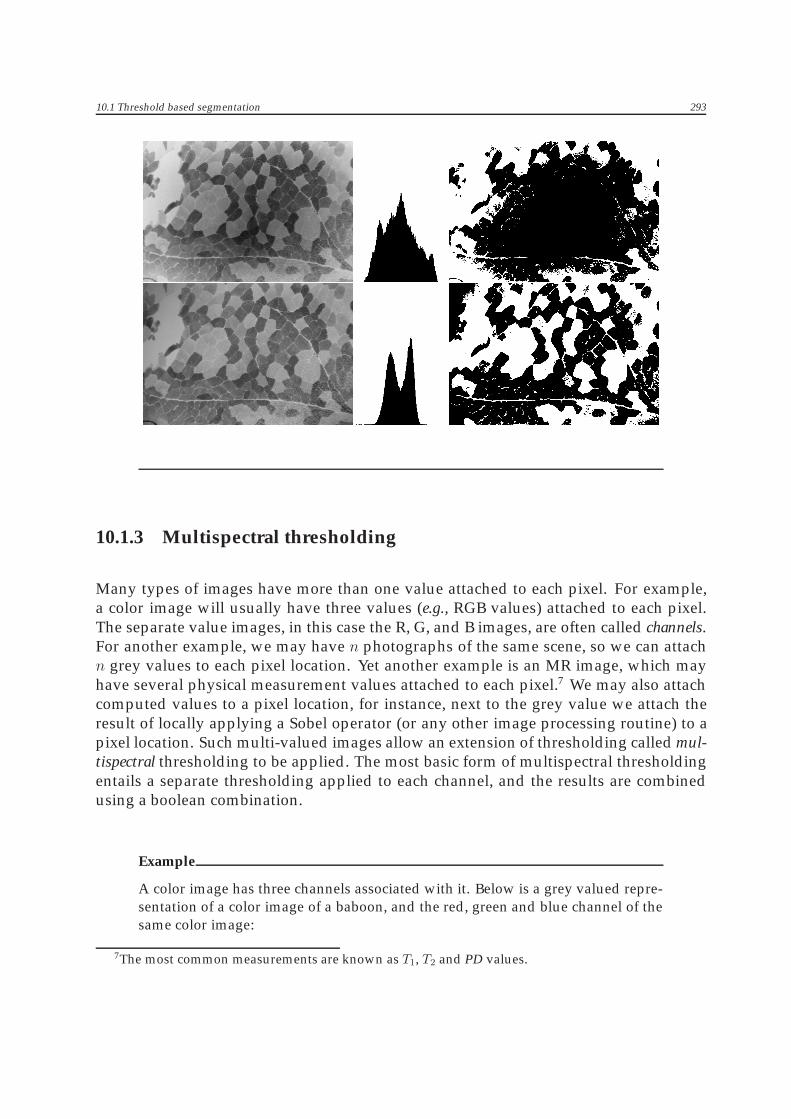
When an image is distorted by a large scale gradient artifact, its histogram willdiffuse, and its entropy will rise. To correct the artifact, we subtract possible artifactimages from the corrupted image until we find a result that has minimal entropy.We will not detail the search process of finding the correct artifact image here, butan example of a light microscope image where the gradient image is removed byminimizing the entropy is given below: the top row shows a corrupted image (withgradient artifact), its histogram and the result of thresholding. The bottom rowshows the same images after correction using histogram entropy minimization.
10.1 Threshold based segmentation 293
10.1.3 Multispectral thresholding
Many types of images have more than one value attached to each pixel. For example,a color image will usually have three values (e.g., RGB values) attached to each pixel.The separate value images, in this case the R, G, and B images, are often called channels.For another example, we may have n photographs of the same scene, so we can attachn grey values to each pixel location. Yet another example is an MR image, which mayhave several physical measurement values attached to each pixel.7 We may also attachcomputed values to a pixel location, for instance, next to the grey value we attach theresult of locally applying a Sobel operator (or any other image processing routine) to apixel location. Such multi-valued images allow an extension of thresholding called mul-tispectral thresholding to be applied. The most basic form of multispectral thresholdingentails a separate thresholding applied to each channel, and the results are combinedusing a boolean combination.
Example
A color image has three channels associated with it. Below is a grey valued repre-sentation of a color image of a baboon, and the red, green and blue channel of thesame color image:
7The most common measurements are known as T1, T2 and PD values.

294 Segmentation
Suppose we wish to find the image parts that are yellow. We know that yellow isa composite of red and green, so we can find the yellow pixels by thresholding thered and green channels: we take all pixels where both the red and green valuesare above a threshold. Unfortunately, white or bright grey pixels also have a highred and green value, as well as a high blue value. To find only yellow pixels, wedemand the blue value to be below a threshold. Below on the left is the result afterthresholding and combining (by a logical ’and’) the red and green channel, and onthe right the result after excluding the pixels with a high blue value: the yellowpixels.
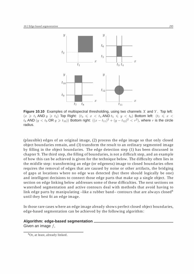
By thresholding each channel separately and combining the results using boolean op-erations, we effectively find segments in rectangular regions of the ’channel space’, asshown in figure 10.10. Channel space is the n-dimensional space (where n is the numberof channels), where each image pixel is plotted using its channel values for coordinates.For example, a pure red pixel has coordinates (1, 0, 0) in the RGB channel space. Thefigure also gives an example of how other regions than rectangles can be segmented bythresholding some function of all channel values.
10.2 Edge based segmentation
Since a (binary) object is fully represented by its edges, the segmentation of an imageinto separate objects can be achieved by finding the edges of those objects. A typicalapproach to segmentation using edges is (1) compute an edge image, containing all
10.2 Edge based segmentation 295
x
x
x
x
y
yy
y
t12
t11
t10
t9
t8t7
t6
t5
t4t3
t2
t1
Figure 10.10 Examples of multispectral thresholding, using two channels X and Y . Top left:(x � t1 AND y � t2) Top Right: (t3 � x < t4 AND t5 � y < t6) Bottom left: (t7 � x <t8 AND (y < t9 OR y � t10)) Bottom right: ((x − t11)2 + (y − t12)2 < r2), where r is the circleradius.
(plausible) edges of an original image, (2) process the edge image so that only closedobject boundaries remain, and (3) transform the result to an ordinary segmented imageby filling in the object boundaries. The edge detection step (1) has been discussed inchapter 9. The third step, the filling of boundaries, is not a difficult step, and an exampleof how this can be achieved is given for the technique below. The difficulty often lies inthe middle step: transforming an edge (or edgeness) image to closed boundaries oftenrequires the removal of edges that are caused by noise or other artifacts, the bridgingof gaps at locations where no edge was detected (but there should logically be one)and intelligent decisions to connect those edge parts that make up a single object. Thesection on edge linking below addresses some of these difficulties. The next sections onwatershed segmentation and active contours deal with methods that avoid having tolink edge parts by manipulating –like a rubber band– contours that are always closed8
until they best fit an edge image.
In those rare cases where an edge image already shows perfect closed object boundaries,edge-based segmentation can be achieved by the following algorithm:
Algorithm: edge-based segmentationGiven an image f ,
8Or, at least, already linked.
296 Segmentation
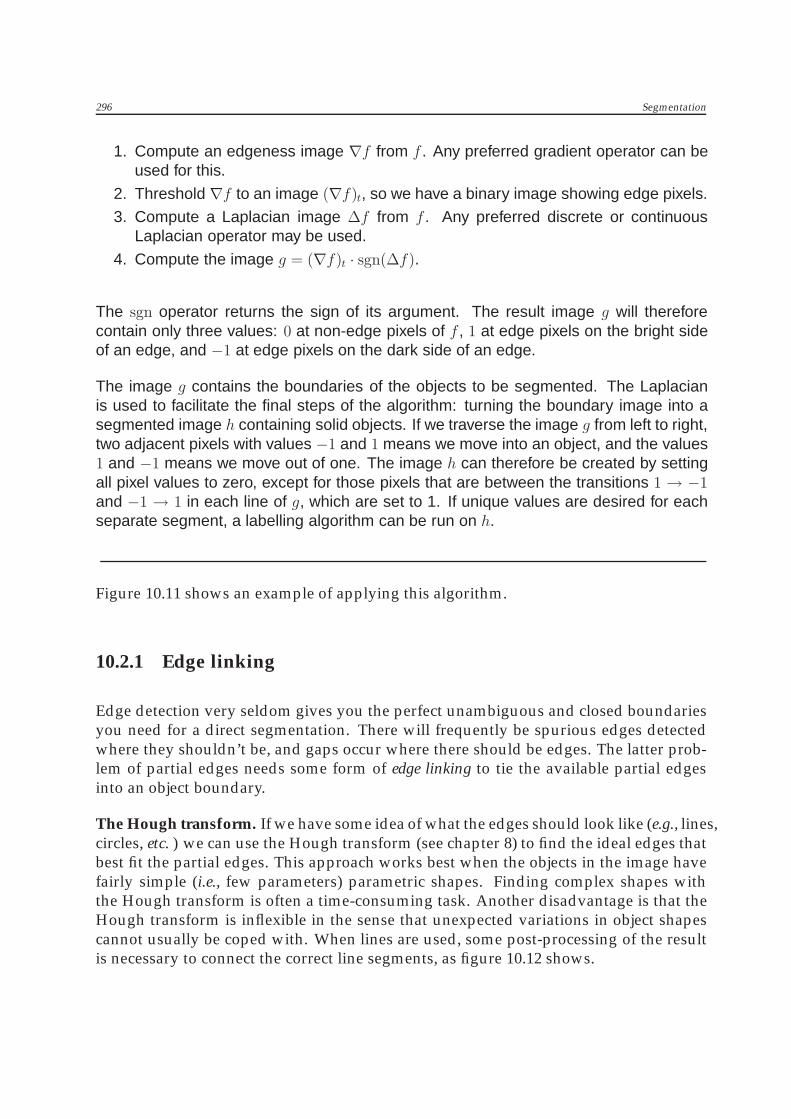
1. Compute an edgeness image ∇f from f . Any preferred gradient operator can beused for this.
2. Threshold ∇f to an image (∇f)t, so we have a binary image showing edge pixels.
3. Compute a Laplacian image Δf from f . Any preferred discrete or continuousLaplacian operator may be used.
4. Compute the image g = (∇f)t · sgn(Δf).
The sgn operator returns the sign of its argument. The result image g will thereforecontain only three values: 0 at non-edge pixels of f , 1 at edge pixels on the bright sideof an edge, and −1 at edge pixels on the dark side of an edge.
The image g contains the boundaries of the objects to be segmented. The Laplacianis used to facilitate the final steps of the algorithm: turning the boundary image into asegmented image h containing solid objects. If we traverse the image g from left to right,two adjacent pixels with values −1 and 1 means we move into an object, and the values1 and −1 means we move out of one. The image h can therefore be created by settingall pixel values to zero, except for those pixels that are between the transitions 1 → −1and −1 → 1 in each line of g, which are set to 1. If unique values are desired for eachseparate segment, a labelling algorithm can be run on h.
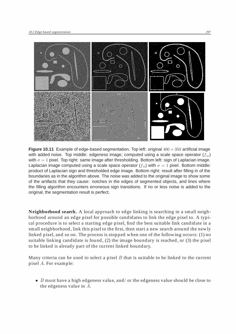
Figure 10.11 shows an example of applying this algorithm.
10.2.1 Edge linking
Edge detection very seldom gives you the perfect unambiguous and closed boundariesyou need for a direct segmentation. There will frequently be spurious edges detectedwhere they shouldn’t be, and gaps occur where there should be edges. The latter prob-lem of partial edges needs some form of edge linking to tie the available partial edgesinto an object boundary.
The Hough transform. If we have some idea of what the edges should look like (e.g., lines,circles, etc. ) we can use the Hough transform (see chapter 8) to find the ideal edges thatbest fit the partial edges. This approach works best when the objects in the image havefairly simple (i.e., few parameters) parametric shapes. Finding complex shapes withthe Hough transform is often a time-consuming task. Another disadvantage is that theHough transform is inflexible in the sense that unexpected variations in object shapescannot usually be coped with. When lines are used, some post-processing of the resultis necessary to connect the correct line segments, as figure 10.12 shows.
10.2 Edge based segmentation 297
Figure 10.11 Example of edge-based segmentation. Top left: original 400× 350 artificial imagewith added noise. Top middle: edgeness image; computed using a scale space operator (fw)with σ = 1 pixel. Top right: same image after thresholding. Bottom left: sign of Laplacian image.Laplacian image computed using a scale space operator (f ii) with σ = 1 pixel. Bottom middle:product of Laplacian sign and thresholded edge image. Bottom right: result after filling in of theboundaries as in the algorithm above. The noise was added to the original image to show someof the artifacts that they cause: notches in the edges of segmented objects, and lines wherethe filling algorithm encounters erroneous sign transitions. If no or less noise is added to theoriginal, the segmentation result is perfect.
Neighborhood search. A local approach to edge linking is searching in a small neigh-borhood around an edge pixel for possible candidates to link the edge pixel to. A typi-cal procedure is to select a starting edge pixel, find the best suitable link candidate in asmall neighborhood, link this pixel to the first, then start a new search around the newlylinked pixel, and so on. The process is stopped when one of the following occurs: (1) nosuitable linking candidate is found, (2) the image boundary is reached, or (3) the pixelto be linked is already part of the current linked boundary.
Many criteria can be used to select a pixel B that is suitable to be linked to the currentpixel A. For example:
• B must have a high edgeness value, and/or the edgeness value should be close tothe edgeness value in A.

298 Segmentation
Figure 10.12 Example of edge linking using the Hough transform. Top left: original noisy256 × 256 image. Top middle: edge image, computed using the fw operator at a scale of σ = 2pixels. Top right: threshold of this image, showing gaps in the object boundary. Bottom left:the Hough transform (lines) of the thresholded edge image, showing eight maxima. Bottommiddle: the corresponding line image of the maxima in the Hough transform. Note that intelligentprocessing of this image is necessary to obtain only those line segments that make up theoriginal object. (In this case we dilated the binary edge image, took the logical ‘and’ with theHough lines image, and performed an opening by reconstruction of erosion.) Bottom right: resultafter processing and filling; we now have a closed boundary.
• The direction of the gradient in B should not differ too much from the gradientdirection in A, and/or the direction from A to B should not differ too much fromthe direction of previous links.
The latter criterion ensures that edges cannot bend too much, which ensures that thesearch is kept on the right path when we reach a point where edges cross. It has alsoproven to be a necessary heuristic for noisy images. A disadvantage, however, is thatedges at places where objects really have sharp angles are not linked. In these cases, apost-processing of all found linked boundary segments is necessary, where the bound-ary segments themselves are linked (using proximity and other criteria) to form closedboundaries. In addition, some form of post-processing is usually necessary to removethose linked edge segments that are unlikely to belong to realistic boundaries. The re-moval criteria are often application dependent, but commonly edge segments below acertain length are removed.
A problem by itself is the proper choice of starting points –the seeds– for the search pro-
10.2 Edge based segmentation 299
cesses. These starting points may be indicated by a user or determined in an application-dependent way. It is also possible to use the (say) hundred points that have the highestedgeness value for starting points. This works well when the contrast of objects andbackground is about the same for all objects. If this is not the case, it may be that nostarting points are picked at low-contrast objects. An approach that remedies this prob-lem is to pick a hundred starting points with highest edgeness values, do edge linking,and then pick a new set of starting points (with highest edgeness), disregarding all pixelstracked in the first run (and possibly their neighborhoods too).
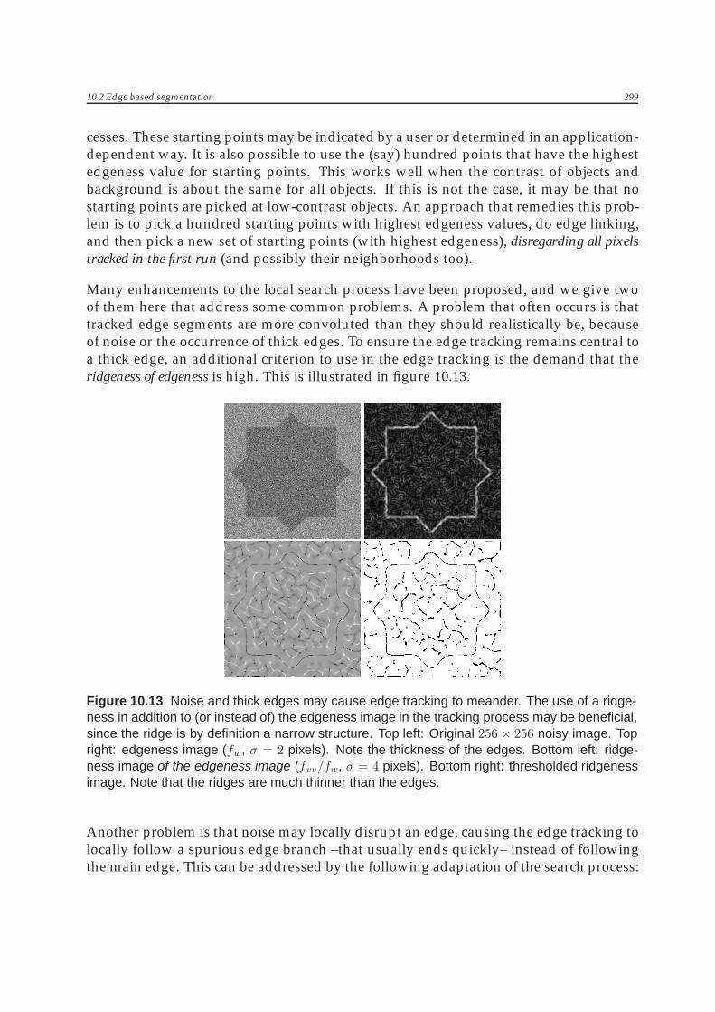
Many enhancements to the local search process have been proposed, and we give twoof them here that address some common problems. A problem that often occurs is thattracked edge segments are more convoluted than they should realistically be, becauseof noise or the occurrence of thick edges. To ensure the edge tracking remains central toa thick edge, an additional criterion to use in the edge tracking is the demand that theridgeness of edgeness is high. This is illustrated in figure 10.13.
Figure 10.13 Noise and thick edges may cause edge tracking to meander. The use of a ridge-ness in addition to (or instead of) the edgeness image in the tracking process may be beneficial,since the ridge is by definition a narrow structure. Top left: Original 256 × 256 noisy image. Topright: edgeness image (fw, σ = 2 pixels). Note the thickness of the edges. Bottom left: ridge-ness image of the edgeness image (fvv/fw, σ = 4 pixels). Bottom right: thresholded ridgenessimage. Note that the ridges are much thinner than the edges.
Another problem is that noise may locally disrupt an edge, causing the edge tracking tolocally follow a spurious edge branch –that usually ends quickly– instead of followingthe main edge. This can be addressed by the following adaptation of the search process:

300 Segmentation
instead of linking an edge pixel to the best linking candidate and then moving on tothis candidate, we make a small list of suitable linking candidates. If linking of the bestcandidate results in a short dead end, we backtrack and see if the next best candidateresults in a longer branch.
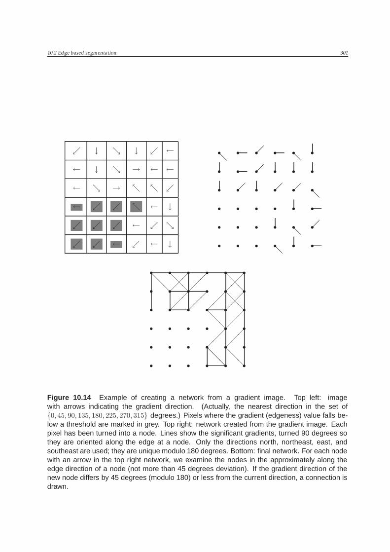
Network analysis: mathematical programming. If we not only have a good startingpoint A for a boundary segment, but also a likely end point B (or a set of potentialend points), then the edge linking process is effectively the same as finding the bestpath from A to B. To find this best path, we first need to construct some network fromwhich all possible paths from A to B can be gleaned. Figure 10.14 shows an exampleof how such a network can be constructed from a gradient image: each edge pixel istransformed to a network node –only pixels with an edgeness value above a certainthreshold are part of the network– and arrows are drawn to all neighboring nodes (pix-els) that can reached from a certain node. An arrow is drawn if certain criteria are met,e.g., the gradient direction at the two nodes does not differ too much.
Our goal now is to find the best path, i.e., the best sequence of arrows, from A to B.’Best’ can be defined in several ways here, depending on the application. The best pathmay, e.g., be the shortest path, the path with highest average edgeness value, the pathwith least curvature, or a combination of these and yet other criteria. These criteriaare included in our network by assigning costs to each arrow. For instance, if we areinterested in the shortest path, we assign distances to each arrow: 1 to each horizontalor vertical arrow,
√2 to each diagonal arrow. If we are interested in a path that is both
short and runs along nodes with high edgeness values, we may assign an arrow costthat is a weighed sum of a distance term and a term inversely proportional to edgeness.The cost of each path from A to B is defined as the sum of costs of the arrows that makethe path. The best path is the path with lowest cost.
The problem of finding the best path has been –and still is– an area of considerableresearch. It is known as the shortest-route problem in the field of operations research, andmany algorithms for (approximately) solving the problem can be found. The problemsolving strategy is known as mathematical programming.9 Other areas of research maypresent the problems under different headings, such as graph searching or networkanalysis. We present here a simple but effective algorithm for finding the best path.
Algorithm: Solving the shortest-route problemProblem: find the shortest route from A to B given a network of nodes and branches,with given distances (costs) for each branch.
The idea of this iterative algorithm is to find the n-th nearest node to A, where n is theiteration number. For example, if n = 1, we find the nearest node to A. If n = 2, we findthe second closest node to A, etc. The algorithm is terminated if the n-th closest nodeis the desired end node B.
9Mathematical programming also contains the techniques indicated as dynamic programming in otherbooks in reference to the problem at hand.
10.2 Edge based segmentation 301
↙ ↓ ↘ ↓ ↙ ←
← ↓ ↘ → ← ←
← ↘ → ↖ ↖ ↙
← ↙ ↙ ↖ ← ↓
↙ ↙ ↙ ← ↙ ↘
↙ ↙ ← ↙ ← ↓ � � � � � �
� � � � � �
� � � � � �
� � � � � �
� � � � � �
� � � � � �
����
��
��
�� �� ����
����
��
� � � � � �
� � � � � �
� � � � � �
� � � � � �
� � � � � �
� � � � � �
��
�
��
�
��
�
��
���
�
��
�
��
�
��
�
��
���
�
��
�
��
��
��
��
�
��
�
��
�
��
�
��
�
Figure 10.14 Example of creating a network from a gradient image. Top left: imagewith arrows indicating the gradient direction. (Actually, the nearest direction in the set of{0, 45, 90, 135, 180, 225, 270, 315} degrees.) Pixels where the gradient (edgeness) value falls be-low a threshold are marked in grey. Top right: network created from the gradient image. Eachpixel has been turned into a node. Lines show the significant gradients, turned 90 degrees sothey are oriented along the edge at a node. Only the directions north, northeast, east, andsoutheast are used; they are unique modulo 180 degrees. Bottom: final network. For each nodewith an arrow in the top right network, we examine the nodes in the approximately along theedge direction of a node (not more than 45 degrees deviation). If the gradient direction of thenew node differs by 45 degrees (modulo 180) or less from the current direction, a connection isdrawn.
302 Segmentation
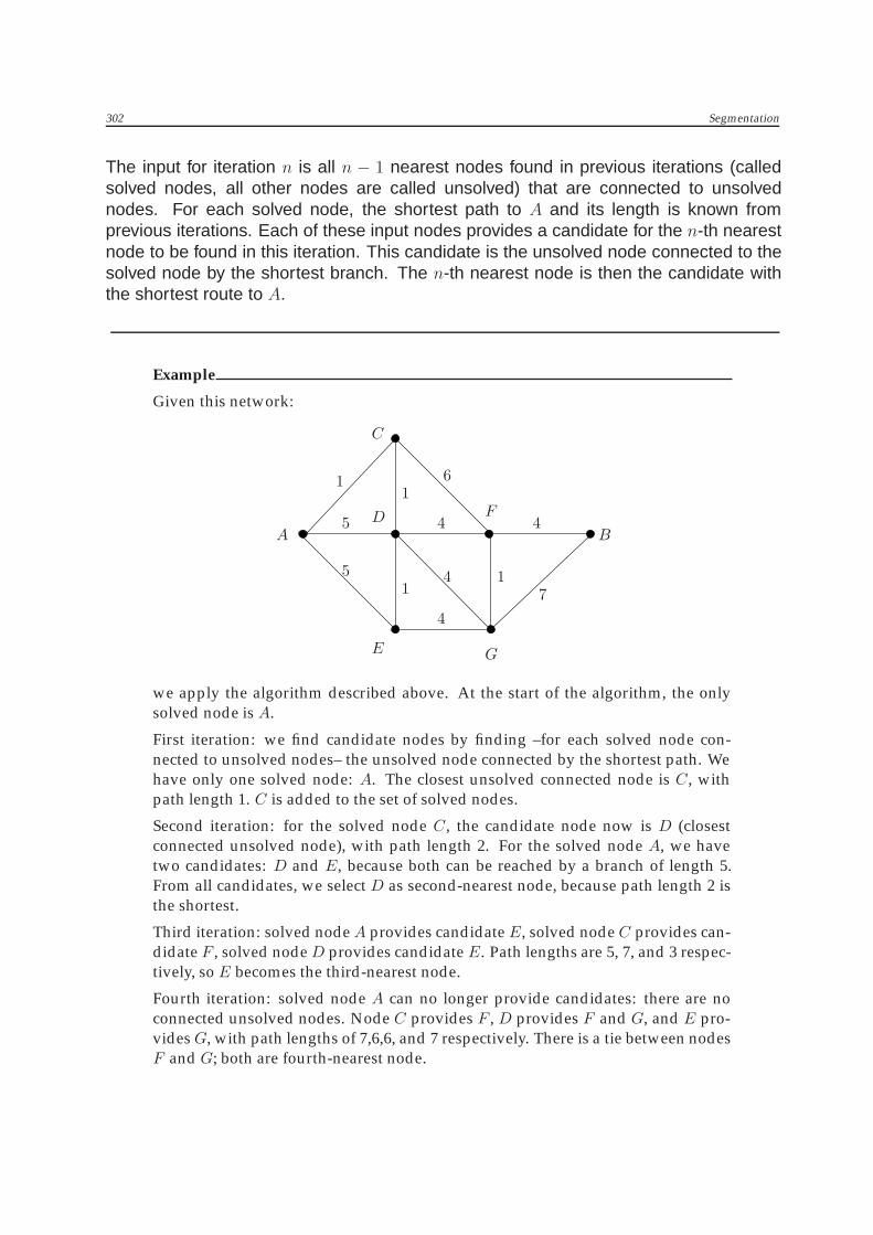
The input for iteration n is all n − 1 nearest nodes found in previous iterations (calledsolved nodes, all other nodes are called unsolved) that are connected to unsolvednodes. For each solved node, the shortest path to A and its length is known fromprevious iterations. Each of these input nodes provides a candidate for the n-th nearestnode to be found in this iteration. This candidate is the unsolved node connected to thesolved node by the shortest branch. The n-th nearest node is then the candidate withthe shortest route to A.
Example
Given this network:
A B
C
D
E
F
G
11
11
4
4
4
4
5
5
6
7
we apply the algorithm described above. At the start of the algorithm, the onlysolved node is A.
First iteration: we find candidate nodes by finding –for each solved node con-nected to unsolved nodes– the unsolved node connected by the shortest path. Wehave only one solved node: A. The closest unsolved connected node is C , withpath length 1. C is added to the set of solved nodes.
Second iteration: for the solved node C , the candidate node now is D (closestconnected unsolved node), with path length 2. For the solved node A, we havetwo candidates: D and E, because both can be reached by a branch of length 5.From all candidates, we select D as second-nearest node, because path length 2 isthe shortest.
Third iteration: solved nodeA provides candidate E, solved node C provides can-didate F , solved nodeD provides candidate E. Path lengths are 5, 7, and 3 respec-tively, so E becomes the third-nearest node.
Fourth iteration: solved node A can no longer provide candidates: there are noconnected unsolved nodes. Node C provides F , D provides F and G, and E pro-videsG, with path lengths of 7,6,6, and 7 respectively. There is a tie between nodesF and G; both are fourth-nearest node.
10.2 Edge based segmentation 303
Fifth iteration: only F and G of the solved nodes have a connected unsolved node,B in both cases. The path lengths are 10 and 13 respectively. B is fifth-nearestnode, and the algorithm terminates.
Backtracking provides us with the optimal path: from B to F toD to C toA; or theright way round: ACDFB.
The table below summarizes the course of the algorithm:
n solved nodes connected closest connected path length n-th nearest nodeto unsolved nodes unsolved node
1 A C 1 C
2 A D 5E 5
C D 1 + 1 = 2 D
3 A E 5C F 1 + 6 = 7D E 2 + 1 = 3 E
4 C F 1 + 6 = 7D F 2 + 4 = 6 F
G 2 + 4 = 6 GE G 3 + 4 = 7
5 F B 6 + 4 = 10 BG B 6 + 7 = 13
10.2.2 Watershed segmentation
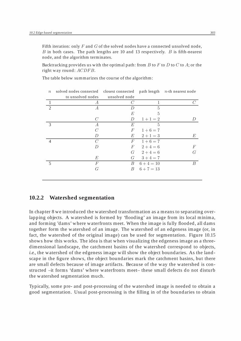
In chapter 8 we introduced the watershed transformation as a means to separating over-lapping objects. A watershed is formed by ‘flooding’ an image from its local minima,and forming ’dams’ where waterfronts meet. When the image is fully flooded, all damstogether form the watershed of an image. The watershed of an edgeness image (or, infact, the watershed of the original image) can be used for segmentation. Figure 10.15shows how this works. The idea is that when visualizing the edgeness image as a three-dimensional landscape, the catchment basins of the watershed correspond to objects,i.e., the watershed of the edgeness image will show the object boundaries. As the land-scape in the figure shows, the object boundaries mark the catchment basins, but thereare small defects because of image artifacts. Because of the way the watershed is con-structed –it forms ‘dams’ where waterfronts meet– these small defects do not disturbthe watershed segmentation much.
Typically, some pre- and post-processing of the watershed image is needed to obtain agood segmentation. Usual post-processing is the filling in of the boundaries to obtain
304 Segmentation
solid segments. In the case of watershed segmentation, we do not need to worry aboutsmall ‘leaks’ in a boundary (a small leak between two segments will fill in the twosegments as being a single segment). Because of the way the watershed is constructed,leaks cannot occur.
Figure 10.15 Example of edgeness watershed segmentation. Top left: original noisy image.Top right: edgeness image. Bottom left: landscape version of the edgeness image. Note thatobjects are surrounded by a ‘palisade’, that will hold the water in the flooding process that formsthe watershed. Dams will be formed when the water level reaches the tops of the palisades.An uneven palisade height will not disturb the formation of the correct dam marking an objectboundary. Bottom right: all dams formed; the watershed of the edgeness image.
Some pre- and post-processing is usually necessary to avoid an oversegmentation. Inthe example in our figure, we set all grey values below a threshold to zero. This en-sures no dams are formed early in the flooding process. Since such dams are causedby very weak edges, they are unlikely to correspond to object boundaries, and shouldnot be part of the segmentation watershed. Our example still shows some oversegmen-tation: besides the correct object boundaries, several erroneous branches are present.Many approaches have been proposed to remove these erroneous branches. One effec-tive method is to merge those segments that are likely to belong together. How thislikelihood is measured is discussed in the section on region based segmentation. An-
10.2 Edge based segmentation 305
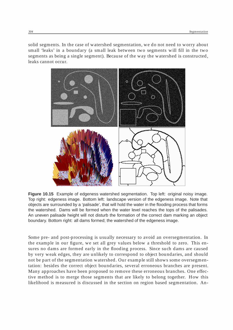
other method that is effective in our example is to compute the average edgeness valueof each branch, and remove those branches where this average falls below a threshold.Figure 10.16 shows that this effectively removes all spurious branches from our exam-ple.
Figure 10.16 Example of removing the spurious branches of the edgeness watershed to reduceoversegmentation of the original image. The image shows a multiplication of the edgenessimage and its watershed from the previous figure, clearly showing that the erroneous branchescan be easily removed by thresholding the average edgeness of branches.
10.2.3 Snakes
An active contour or snake is a curve defined in an image that is allowed to change itslocation and shape until it best satisfies predefined conditions. It can be used to segmentan object by letting it settle –much like a constricting snake– around the object boundary.
A snake C is usually modeled as a parametrized curve C(s) = (x(s), y(s)), where theparameter s varies from 0 to 1. So, C(0) gives the coordinate pair (x(0), y(0)) of the start-ing point, C(1) gives the end coordinates, and C(s) with 0 < s < 1 gives all intermediatepoint coordinates. The movement of the snake is modeled as an energy minimizationprocess, where the total energy E to be minimized consists of three terms:
E =
1∫0
E(C(s))ds =
1∫0
(Ei(C(s)) + Ee(C(s)) + Ec(C(s))
)ds.
The term Ei is based on internal forces of the snake; it increases if the snake is stretchedor bent. The term Ee is based on external forces; it decreases if the snake moves closer toa part of the image we wish it to move to. For example, if we wish the snake to move to

306 Segmentation
edges, we may base this energy term on edgeness values. The last term Ec can be usedto impose additional constraints, such as penalizing the creation of loops in the snake,penalizing moving too far away from the initial position, or penalizing moving into anundesired image region. For many applications, Ec is not used, i.e., simply set to zero.Common definitions for the internal and external terms are
Ei = c1
∥∥∥dC(s)ds
∥∥∥2
+ c2
∥∥∥d2C(s)ds2
∥∥∥2
Ee = −c3 ‖∇f‖2 ,
where the external term is based on the assumption that the snake should be attractedto edges of the original image f . By using other external terms, we can make use ofdifferent image features, making the snake follow ridges, find corner points, etc. Theconstants c1, c2, and c3 determine the relative influence of each term on the movementof the snake. The elasticity of the snake is controlled by c1; the norm of the derivativedC(s)ds
measures how much the snake is stretched locally, so setting c1 to zero will resultin high stretch values having no impact on the energy, hence the snake may stretchinfinitely. Alternatively, a high (relative to the other c’s) value of c1 makes that thesnake can stretch very little. In the same manner, c2 controls how much the snake canbend (i.e., its stiffness or rigidity), since the second derivative d2C(s)
ds2is a measure for the
snake’s curvature, and c3 sets the relative influence of the edge attraction force.
When implementing a snake, it is commonly modeled by a connected series of splines.This model allows the snake –on the one hand– to be easily connected to the mathemat-ical model: the spline representation is easily converted to the parametrized curve C(s),and its derivatives can also be computed in a straightforward manner. On the otherhand, the discrete set of control points of the spline give a handle to optimizing thesnake; only the control points need to be moved, and the set is easily related to discreteimages. The optimization itself is not usually carried out by direct minimization of theenergy functional E, but by numerically solving its Euler-Lagrange form:
− d
ds
(c1
∥∥∥∥dC(s)
ds
∥∥∥∥2)
+d2
ds2
(c2
∥∥∥∥d2C(s)
ds2
∥∥∥∥2)
+∇(Ee + Ec) = 0.
Figure 10.17 shows an example of a snake used to find the boundary of an object.
For a snake to converge to the desired location and shape, we need a good starting esti-mate in most practical applications. This can be provided by the user, or by processingand linking of extracted edges as described in the previous section. To improve thechances of the snake converging to the desired shape, many current algorithms haveadded features to the original snake algorithm, such as:
10.2 Edge based segmentation 307
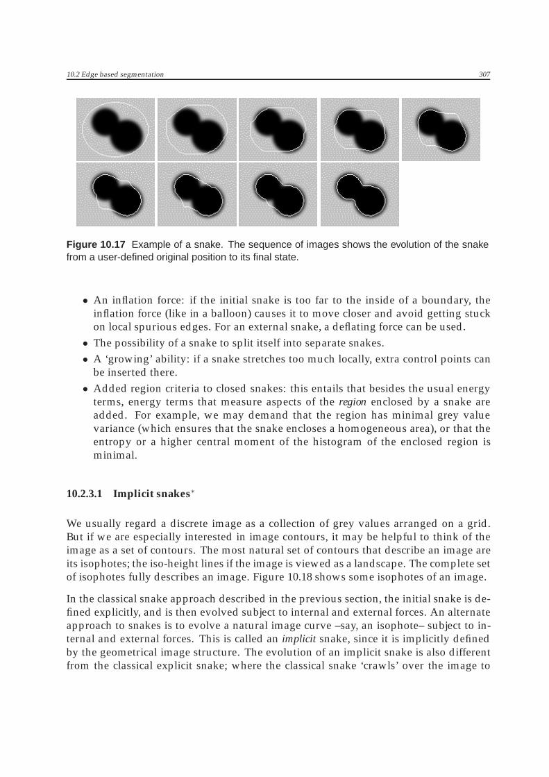
Figure 10.17 Example of a snake. The sequence of images shows the evolution of the snakefrom a user-defined original position to its final state.
• An inflation force: if the initial snake is too far to the inside of a boundary, theinflation force (like in a balloon) causes it to move closer and avoid getting stuckon local spurious edges. For an external snake, a deflating force can be used.• The possibility of a snake to split itself into separate snakes.• A ‘growing’ ability: if a snake stretches too much locally, extra control points can
be inserted there.• Added region criteria to closed snakes: this entails that besides the usual energy
terms, energy terms that measure aspects of the region enclosed by a snake areadded. For example, we may demand that the region has minimal grey valuevariance (which ensures that the snake encloses a homogeneous area), or that theentropy or a higher central moment of the histogram of the enclosed region isminimal.
10.2.3.1 Implicit snakes∗
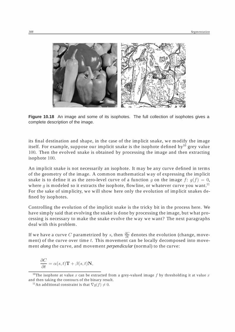
We usually regard a discrete image as a collection of grey values arranged on a grid.But if we are especially interested in image contours, it may be helpful to think of theimage as a set of contours. The most natural set of contours that describe an image areits isophotes; the iso-height lines if the image is viewed as a landscape. The complete setof isophotes fully describes an image. Figure 10.18 shows some isophotes of an image.
In the classical snake approach described in the previous section, the initial snake is de-fined explicitly, and is then evolved subject to internal and external forces. An alternateapproach to snakes is to evolve a natural image curve –say, an isophote– subject to in-ternal and external forces. This is called an implicit snake, since it is implicitly definedby the geometrical image structure. The evolution of an implicit snake is also differentfrom the classical explicit snake; where the classical snake ‘crawls’ over the image to
308 Segmentation
Figure 10.18 An image and some of its isophotes. The full collection of isophotes gives acomplete description of the image.
its final destination and shape, in the case of the implicit snake, we modify the imageitself. For example, suppose our implicit snake is the isophote defined by10 grey value100. Then the evolved snake is obtained by processing the image and then extractingisophote 100.
An implicit snake is not necessarily an isophote. It may be any curve defined in termsof the geometry of the image. A common mathematical way of expressing the implicitsnake is to define it as the zero-level curve of a function g on the image f : g(f) = 0,where g is modeled so it extracts the isophote, flowline, or whatever curve you want.11
For the sake of simplicity, we will show here only the evolution of implicit snakes de-fined by isophotes.
Controlling the evolution of the implicit snake is the tricky bit in the process here. Wehave simply said that evolving the snake is done by processing the image, but what pro-cessing is necessary to make the snake evolve the way we want? The next paragraphsdeal with this problem.
If we have a curve C parametrized by s, then ∂C∂t
denotes the evolution (change, move-ment) of the curve over time t. This movement can be locally decomposed into move-ment along the curve, and movement perpendicular (normal) to the curve:
∂C
∂t= α(s, t)T + β(s, t)N,
10The isophote at value x can be extracted from a grey-valued image f by thresholding it at value xand then taking the contours of the binary result.
11An additional constraint is that ∇g(f) = 0.

10.2 Edge based segmentation 309
where T and N are the local tangential and normal unit vectors to the curve, and α andβ are arbitrary functions. Tangential movement, however, does not alter the curve,12
so we can effectively write the curve evolution as an evolution in the normal directiononly:
∂C
∂t= β ′(s, t)N,
where β ′ depends only on α and β. Without proof, we note her that if the curve C isan isophote of the image f , then the curve evolution can be written in terms of imageevolution by the equivalence:
∂C
∂t= β ′(·)N ⇐⇒ ∂f
∂t= −fwβ ′(·),
where we use the local gradient-based coordinate system (v, w) defined in chapter 9.The arguments of β′ on the left side must be ‘translated’ to arguments in image form.This is not a trivial matter in general. A frequently occurring argument is the isophotecurvature κ, which (as we have seen before) can be expressed as−fvv/fw. Table 10.1 listssome frequently used curve evolutions. Note that we have seen the image evolutionequations before as the equations driving non-linear diffusion in chapter 9.
Curve evolution Image evolution∂C∂t
= cN ∂f∂t
= cfw∂C∂t
= κN ∂f∂t
= fvv∂C∂t
= (α + βκ)N ∂f∂t
= αfw + βfvv∂C∂t
= κ1/3N ∂f∂t
= f1/3vv f
2/3w
Table 10.1 Some examples of implicit snake curve evolution equations and the correspondingimage evolution equations.
A type of implicit snake that can be used well for many segmentation tasks is controlledby the equation ∂C
∂t= gκN−∇g, where g is a function that decreases with edgeness (such
as g = exp(
−f2w
k2
)), and κ is the isophote curvature. The image evolution form is ∂f
∂t=
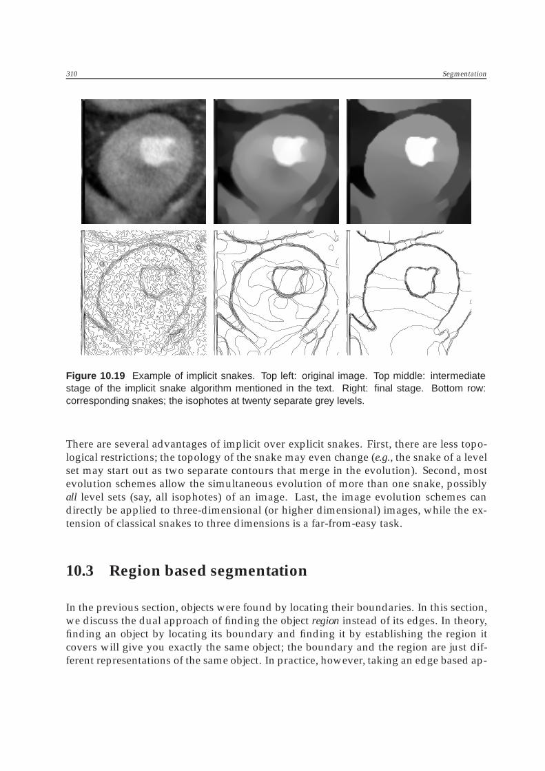
gfvv+∇g ·∇f . Without going into the mathematical explanation, we note that this snakewill be attracted to edges in such a way that evolving an image will result in an imagewhere segmentation can optimally be done using simple thresholding. Figure 10.19shows an example of this.
12Only its parameterization.
310 Segmentation
Figure 10.19 Example of implicit snakes. Top left: original image. Top middle: intermediatestage of the implicit snake algorithm mentioned in the text. Right: final stage. Bottom row:corresponding snakes; the isophotes at twenty separate grey levels.
There are several advantages of implicit over explicit snakes. First, there are less topo-logical restrictions; the topology of the snake may even change (e.g., the snake of a levelset may start out as two separate contours that merge in the evolution). Second, mostevolution schemes allow the simultaneous evolution of more than one snake, possiblyall level sets (say, all isophotes) of an image. Last, the image evolution schemes candirectly be applied to three-dimensional (or higher dimensional) images, while the ex-tension of classical snakes to three dimensions is a far-from-easy task.
10.3 Region based segmentation
In the previous section, objects were found by locating their boundaries. In this section,we discuss the dual approach of finding the object region instead of its edges. In theory,finding an object by locating its boundary and finding it by establishing the region itcovers will give you exactly the same object; the boundary and the region are just dif-ferent representations of the same object. In practice, however, taking an edge based ap-
10.3 Region based segmentation 311
proach to segmentation may give radically different results than taking a region basedapproach. The reason for this is that we are bound to using imperfect images and imper-fect methods, hence the practical result of locating an object boundary may be differentfrom locating its region.
Region based segmentation methods have only two basic operations: splitting and merg-ing, and many methods even feature only one of these. The basic approach to imagesegmentation using merging is:
1. obtain an initial (over)segmentation of the image,2. merge those adjacent segments that are similar –in some respect– to form single
segments,3. go to step 2 until no segments that should be merged remain.
The initial segmentation may simply be all pixels, i.e., each pixel is a segment by itself.The heart of the merging approach is the similarity criterion used to decide whetheror not two segments should be merged. This criterion may be based on grey valuesimilarity (such as the difference in average grey value, or the maximum or minimumgrey value diference between segments), the edge strength of the boundary between thesegments, the texture of the segments, or one of many other possibilities.
The basic form of image segmentation using splitting is:
1. obtain an initial (under)segmentation of the image,2. split each segment that is inhomogeneous in some respect (i.e., each segment that
is unlikely to really be a single segment).3. go to step 2 until all segments are homogeneous.
The initial segmentation may be no segmentation at all, i.e., there is only a single seg-ment, which is the entire image. The criterion for inhomogeneity of a segment may bethe variance of its grey values, the variance of its texture, the occurrence of strong in-ternal edges, or various other criteria. The basic merging and splitting methods seemto be the top-down and bottom-up approach to the same method of segmentation, butthere is an intrinsic difference: the merging of two segments is straightforward, but thesplitting of a segment requires we establish suitable sub-segments the segments can besplit into. In essence, we still have the segmentation problem we started with, except itis now defined on a more local level. To avoid this problem, the basic splitting approachis often enhanced to a combined split and merge approach, where inhomogeneous seg-ments are split into simple geometric forms (usually into four squares) recursively. Thisof course creates arbitrary segment boundaries (that may not be correlated to realisticboundaries), and merge steps are included into the process to remove incorrect bound-aries.
312 Segmentation
10.3.1 Merging methods
Region growing. Many merging methods of segmentation use a method called regiongrowing to merge adjacent single pixel segments into one segment. Region growingneeds a set of starting pixels13 called seeds. The region growing process consists of pick-ing a seed from the set, investigating all 4-connected neighbors of this seed, and merg-ing suitable neighbors to the seed. The seed is then removed from the seed set, andall merged neighbors are added to the seed set. The region growing process continuesuntil the seed set is empty. The algorithm below implements an example with a singleseed, where all connected pixels with the same grey value as the seed are merged.
Algorithm: Region growingThe data structure used to keep track of the set of seeds is usually a stack. Two opera-tions are defined on a stack: push, which puts a pixel (or rather, its coordinates) on thetop of the stack, and pop, which takes a pixel from the top of the stack.
In the algorithm, the image is called f , the seed has coordinates (x, y) and grey valueg = f(x, y). The region growing is done by setting each merged pixel’s grey value to avalue h (which must not equal g). The pixel under investigation has coordinates (a, b).The algorithm runs:
1. push (x, y)
2. as long as the stack is not empty do
(a) pop (a, b)
(b) if f(a, b) = g theni. set f(a, b) to h
ii. push (a− 1, b)
iii. push (a+ 1, b)
iv. push (a, b− 1)
v. push (a, b+ 1)
The final region can be extracted from the image by selecting all pixels with grey valueh. To ensure the correctness of the result, we must select h to be a value that is notpresent in the original image prior to running the algorithm. The statement that decidesif a pixel should be merged (‘if f(a, b) = g’) can be modified to use a different mergingcriterion. A simple modification would be to allow merging of pixels that are in a certainrange of grey values (‘if l < f(a, b) < h’). An example of this is shown in figure 10.20.
13Which usually contains only a single pixel.
10.3 Region based segmentation 313
Another modification is to allow merging only if the gradient value of the candidatepixel is low (a high gradient could signify we are at the edge of an object). This last cri-terion is often combined with a grey value range criterion to ensure the region growingdoes not grow right through a weak spot in the boundary where the gradient value islow. More elaborate merging criteria can be used, but they do not usually result in asgood a segmentation as may be hoped for, since the heart of region growing is the eval-uation of the criterion at a single pixel –the merging candidate– which may be prone tonoise. Elaborate criteria are usually more effectively used when evaluating whether tomerge two segments of a larger size.
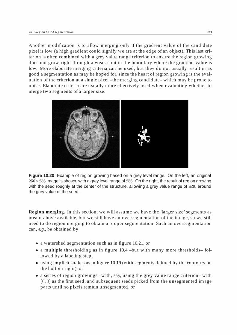
Figure 10.20 Example of region growing based on a grey level range. On the left, an original256×256 image is shown, with a grey level range of 256. On the right, the result of region growingwith the seed roughly at the center of the structure, allowing a grey value range of ±30 aroundthe grey value of the seed.
Region merging. In this section, we will assume we have the ‘larger size’ segments asmeant above available, but we still have an oversegmentation of the image, so we stillneed to do region merging to obtain a proper segmentation. Such an oversegmentationcan, e.g., be obtained by
• a watershed segmentation such as in figure 10.21, or• a multiple thresholding as in figure 10.4 –but with many more thresholds– fol-
lowed by a labeling step,• using implicit snakes as in figure 10.19 (with segments defined by the contours on
the bottom right), or• a series of region growings –with, say, using the grey value range criterion– with
(0, 0) as the first seed, and subsequent seeds picked from the unsegmented imageparts until no pixels remain unsegmented, or
314 Segmentation
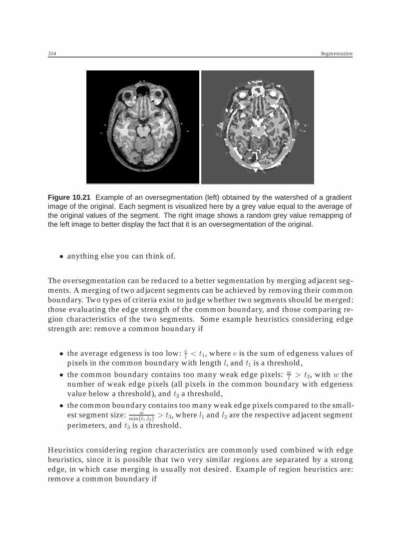
Figure 10.21 Example of an oversegmentation (left) obtained by the watershed of a gradientimage of the original. Each segment is visualized here by a grey value equal to the average ofthe original values of the segment. The right image shows a random grey value remapping ofthe left image to better display the fact that it is an oversegmentation of the original.
• anything else you can think of.
The oversegmentation can be reduced to a better segmentation by merging adjacent seg-ments. A merging of two adjacent segments can be achieved by removing their commonboundary. Two types of criteria exist to judge whether two segments should be merged:those evaluating the edge strength of the common boundary, and those comparing re-gion characteristics of the two segments. Some example heuristics considering edgestrength are: remove a common boundary if
• the average edgeness is too low: el< t1, where e is the sum of edgeness values of
pixels in the common boundary with length l, and t1 is a threshold,• the common boundary contains too many weak edge pixels: w
l> t2, with w the
number of weak edge pixels (all pixels in the common boundary with edgenessvalue below a threshold), and t2 a threshold,• the common boundary contains too many weak edge pixels compared to the small-
est segment size: wmin{l1,l2} > t3, where l1 and l2 are the respective adjacent segment
perimeters, and t3 is a threshold.
Heuristics considering region characteristics are commonly used combined with edgeheuristics, since it is possible that two very similar regions are separated by a strongedge, in which case merging is usually not desired. Example of region heuristics are:remove a common boundary if
10.3 Region based segmentation 315
• the grey values of the adjacent regions are similar. Various measures can be usedto measure this, e.g.,
– the average grey value of the two segments differs by less than a threshold:|g1 − g2| < t1,
– the maximum (or minimum) grey value difference found between the twosegments is below a threshold: max(x1,y1)∈S1,(x2,y2)∈S2 |g(x1, y1)−g(x2, y2)| < t2,
– in addition to one of the above measures: the variance of grey values in eachsegment must be similar: |σ2(S1)− σ2(S2)| < t3, or |Δ(S1)−Δ(S2)| < t4,
• the texture of the regions is similar. Example of texture measures are treated in aseparate section later in this chapter.• the histogram of the adjacent segments is similar. The similarity can be measured
by comparing scalar histogram features such as (central) moments or entropy ofthe histogram. Note that comparing first and second (central) histogram momentsboils down to the same average and variance grey value criteria as describedabove.
In the above, S1 and S2 denote the respective segment regions, g is a grey value, gi is theaverage grey value of segment i, tj is a threshold, σ2(Si) denotes the grey value variance,and Δ(Si) is the maximum grey value difference occurring in segment i. Combinationsof the criteria above are also possible. The removal of common boundaries is usuallydone recursively: all common boundaries in an image are considered for removal, thosethat do not meet the set criteria are removed, and the process is repeated until no morecommon boundaries are removed. Note that the order in which the common boundariesare removed may have an impact on the merging process: suppose we have three seg-ments S1, S2, and S3, with the pairs (S1, S2) and (S2, S3) adjacent. Then merging S1 andS2 to a new segment S12 may cause that S12 and S3 are unsuitable for merging, whilepreviously S2 and S3 were to be merged according to the criteria set. In practice, it is of-ten a good idea to start by removing the weakest boundary, re-evaluating the boundarystrengths, again remove the weakest, etc. .
10.3.2 Splitting and split & merge methods
Where region merging is an agglomerative approach, region splitting is divise. We men-tioned before that this difference makes that the two approaches are not opposites, butfundamentally different problems; the merging of two segments is straightforward, butthe splitting of a segment requires that suitable sub-segments are established to split theoriginal segment into. The problem of how to split a segment is of course itself a segmen-tation problem, and we can treat it as such: any segmentation method (such as the onestreated in this chapter) can be applied to the segment to establish sub-segments. Besidesthe hierarchical level, there is no intrinsic difference The problem of how to decide if a

316 Segmentation
segment need splitting can be solved using the same measures of region homogeneitymentioned in the section on region merging, e.g., a segment needs to be split if
• the grey value variance exceeds a threshold, or• the variance of a texture measure exceeds a threshold, or• the histogram entropy (or another histogram measure) exceeds a threshold, or• high edgeness pixels are present.
When a segment needs splitting, a faster approach than starting a segmentation on thesegment is to simply split it into four quadrants. This of course has a high probability ofplacing segment boundaries at unrealistic positions. This problem is reduced by addingmerging operations to the segmentation process; recursively splitting and merging theimage segments in a way such as the one used in figure 10.22. Especially if different
Figure 10.22 Example of split and merge segmentation. Left: original image. From left toright: recursively splitting each segment into four segments when the grey value variance of asegment is non-zero. If we subsequently recursively merge all adjacent segments with the same(average) grey value, we end up with two segments; exactly the desired segments of object andbackground.
criteria are used for splitting and merging –for example, edge heuristics for the merg-ing and region homogeneity for splitting– the split and merge segmentation may notconverge to a stable result, but instead keep alternating between various solutions. Thisproblem can sometimes be avoided by modifying the criteria in the course of the pro-cess, but is usually simply ignored by terminating the process after a fixed number ofiterations. Another problem of the ‘split into quadrants and merge’ approach is that theresulting segmentation may be very blocky. Figure 10.23 shows examples of using thisapproach.
10.3.3 Pyramid, tree, and scale space methods
Trees are often used as data structures that represent segmentation by splitting andmerging. For example, figure 10.24 shows there is an easy one-to-one relationship be-
10.3 Region based segmentation 317
tween splitting an image recursively into quadrants and a quadtree, as we have seenpreviously in section 8.3.7. The quadtree is often a more convenient and efficient datastructure to use in a segmentation by splitting than the image itself. However, using atree of this type is limited, because we cannot –for instance– model a merging of twosegments on different levels of the pyramid. A more common use of a tree structure isto use it in combination with a multiresolution pyramid (or a scale space): the pyramidlevel defines the tree level, each pixel in the pyramid defines a tree node, and branchescan be formed between nodes in adjacent levels. In this context, a branch is usuallycalled a link, the high-level end a parent, and the other end a child. An example of sucha pyramid-tree can be seen in figure 10.25. Ways to construct a pyramid have beendiscussed in section9.3.
There are many ways to construct and use a pyramid-tree for segmentation, but allapproaches share three steps:
• creating the multiresolution pyramid,• creating links,• finding nodes whose leaves (i.e., connected nodes on the base pyramid level) iden-
tify a segment. Such nodes are called roots.
Many methods iterate between the various steps, e.g., the pyramid may be re-createdusing the results of the first linking step. In this section, we will show two examples ofpyramid-tree segmentation; a classical approach (Burt-pyramid) and an advanced oneusing scale space techniques.
A classical example. The initial pyramid is created by averaging of the grey values ofeach 4 × 4 neighborhood. Links are created upwards from the base level of the pyra-mid. Each child is given exactly one link upwards, to the candidate parent in the 4 × 4neighborhood that is closest in grey value. The pyramid is then re-created by assigningto each pixel the average grey value of its children–the base level remains unmodified.The linking and re-creation is iterated to stability. A segmentation is obtained by go-ing down the final pyramid-tree until the number of nodes on the current level equalsthe pre-defined number of desired segments. These nodes are then assigned to be thesegment roots, and the leaves of their sub-trees constitute the various segments.
Example
For reasons of clarity, we show here a one-dimensional example of the algorithmdescribed above. We have image data of a noisy edge; the subsequent 16 greyvalues are {6, 6, 6, 0, 4, 22, 16, 26, 26, 16, 26, 38, 18, 28, 16, 28}. From this data, we canconstruct the following pyramid by averaging each 4 grey values. Each pyramidlevel reduces resolution by a factor of two. Lines show which children where usedin the computation of each parent.

318 Segmentation
6 6 6 0 4 22 16 26 26 16 26 36 18 28 16 28
6 4 11 23 24 24 25 24
7 16 24 24
16 21
19
Now we link each child to the parent in the 4×4 neighborhood on the current levelthat is closest in grey value. In case of a tie between candidate parents, we link tothe spatially closest parent:
6 6 6 0 4 22 16 26 26 16 26 36 18 28 16 28
6 4 11 23 24 24 25 24
7 16 24 24
16 21
19
Actually, an additional heuristic was used in the linking process that avoids thecrossing of links (‘22’ and ‘36’ grey values on the base level). When this happens,one of the crossing links is destroyed, and the child is linked to the next closestparent. Now we recompute the pyramid values: each parent is given the averagevalue of its children. Parents without children are deleted from the tree.
6 6 6 0 4 22 16 26 26 16 26 36 18 28 16 28
6 2 23 27 22
25 25
17
19 28
9
9 25
Since a repetition of the linking process does not alter the tree, we terminate theprocess. The segmentation of the image can now be done by bunching all the leavesof the sub-trees at an appropriate pyramid level. For example, if we desire twosegments, we take the second level from the top: the sub-tree with root ‘9’ definesone segment, and the sub-tree with root ‘25’ defines the other. Segmentation atlower pyramid levels gives us respectively three, seven, and 16 segments.
10.3 Region based segmentation 319
A pyramid-tree segmentation using scale space. In this example, the pyramid levelsare taken from a scale space built of the original image. The advantage of using scalespace is that it is easier to control the reduction of resolution between two pyramid lev-els. In the pyramid in the previous example, the resolution in each spatial dimensionwas reduced by a factor of two if we move up a level in the pyramid. In a formula:14
Nn = 12Nn−1, where Ni is the number of pixels in one dimension at level i of the pyra-
mid, the base level being level 0. In terms of the original number of pixels, this becomesNn =
(12
)nN0. In scale space, the story is a bit more complex: although scaling an image
lowers its intrinsic resolution, it is common practice to represent the scaled image usingthe same number of pixels as in the original image, instead of the more natural numberof pixels that is inversely proportional to the scale of the image.15 This is not very prac-tical in our case; we need a decreasing number of pixels as we rise in the pyramid/scalespace. To achieve this, we subsample scaled images. The correct subsampling rate andthe correct scale σn of each pyramid level are related by the equations:
σn = εeτ0+nδ
Nn = N0e−nδ,
where δ is a scale sampling parameter and ε is the pixel distance in the original image.The constant τ0 is used to relate ε to the inner scale of the original image. Often τ0 isassumed to be zero, which gives us σ0 = ε for the original image, i.e., the inner scale ofthe original image equals the pixel size. The example below shows how we can build apyramid for segmentation based on scale space.
Example
Suppose we wish to construct a pyramid using scale space where the resolutionin each spatial dimension is reduced by a factor of two if we go up a level. Thenthe following holds (see text above for an explanation): Nn =
(12
)nN0. We also
know that Nn = N0e−nδ. Some calculation then leads to δ = ln 2. Substituting this
in σn = εeτ0+nδ –where we set ε to 1 (i.e., distances are measured in original pixellengths), and take τ0 to be zero– we arrive at σn = 2n.
We now have almost everything to compute pyramid based on scale space of, say,a 256 × 256 image: the base of the pyramid is the original image. The first levelis created by computing the image at scale σ = 21 = 2, and subsampling it using128 × 128 pixels. Level two is created by taking the image at scale σ = 22 = 4, andsubsampling it at 64 × 64. And so on, until the desired number of pyramid levelsis reached.
There is only one snag: scaled images must be computed based on the originalimage, which we assumed to have scale σ = 1. We must compensate for this ‘offset’
14For simplicity, we assume that the original resolution is a power of 2.15More accurately, the number of pixels along each spatial axis (i.e., the x-dimension and y-dimension
of the image) is inversely proportional to the scale.

320 Segmentation
scale when computing the pyramid levels. We can do this by using the formula
σc =√σ2a + σ2
b , where σc is the scale of an image with original scale σa whenconvolved with a Gaussian of width σb. For example, pyramid level 1, with scaleσ = 2, is computed by applying convolution with a Gaussian with scale σ =
√3 to
the original image, because then the final scale σ1 will be σ1 =√
(√
3)2 + 12 = 2.
The example above shows how a pyramid can be constructed with a resolution reduc-tion of a factor of two when rising a level in the pyramid. We chose this example be-cause it creates a pyramid similar to the ‘ordinary’ multiresolution pyramid. For manypractical applications, however, the reduction by a factor of two per level is too fast togive satisfactory segmentation results. Using the scale space approach, we now have aneasy mechanism to set the resolution reduction per level to a lower value: simply setthe variable δ to a lower value (1
2ln 2 instead of ln 2 is a much used heuristic value) and
evaluate the pyramid as in the example above.
After creating the pyramid, the next steps of creating links and finding roots are ba-sically the same as in the Burt-pyramid example. The only intrinsic difference in thelinking process is that we need to establish a set of candidate parents a child may linkto. A common procedure is to examine all parents in a circular region directly abovethe child, with a radius that is proportional to the scale of the parent level. A heuristicvalue for the proportionality constant is 2.5.
Linking criteria. In our first pyramid example, a child was linked to the parent thatwas closest in grey value. For a more effective segmentation, it is for many applicationsbeneficial to use other linkage criteria in addition to the grey value difference. Examplesinclude many of the criteria we have seen before:
• gradient magnitude; a large gradient magnitude (i.e., indication of an edge) of aparent should reduce the probability of a child linking to that parent,• average grey value of the leaves of the sub-tree of a child; this should be close to
the grey value of the parent• spatial distance of child to a potential parent; a large distance should reduce the
link probability.
Probabilistic segmentation. Up until now, we linked children to a single parent only.An interesting addition to the segmentation method is to allow children to link to sev-eral parents, assigning a link strength to each link in such a way that the combinedstrength of all links leaving a child is one; so-called probabilistic linking. Although thisaddition makes the process and implementation more complex, the amount of informa-tion gained over conventional single-linking is considerable: by forcing a child to have
10.3 Region based segmentation 321
only a single parent, you essentially throw away most of the available local information,reducing it to a single binary link. The cumulative loss of information considering allchildren and pyramid levels is substantial. This information loss is not present whenprobabilistic linking is applied.
When a pyramid-tree is probabilistically linked, and we have identified roots that indi-cate segments in the tree, a leaf of the pyramid (i.e., a base level pixel) may no longer beuniquely connected to a single root. Instead, we can compute the probability of a leafbelonging to a particular root. This probability equals the sum of the edge strength ofall paths leading from the root to the leaf via links. The strength of each path equals theproduct of the link strengths of the links in the path.
Probabilistic segmentation allows for a more realistic image segmentation in many cases.For example, suppose we have three pixels in a row: the left pixel is inside an object, theright on the outside, and the middle one straddling the object boundary. Conventionalsegmentation techniques will assign the middle pixel either as object or backgroundpixel16, which is clearly wrong. Probabilistic segmentation will assign the pixel par-tially to the object, and partially to the background, which is much more realistic. Ex-amples of probabilistic segmentation are shown in figure 10.26 and figure 10.27. Usinga probabilistic segmentation is often little more complex than using a conventional one.For example: in non-probabilistic methods, the volume of a segment is determined bycounting all pixels contained in the segment. The probabilistic volume is determinedby counting each pixel for the fraction that it belongs to the segment. Another example:visualization of the surface of segments obtained by non-probabilistic segmentation of-ten gives a ‘blocky’ result. By making pixels on the surface that have a lower segmentprobability partially transparent, the visualization is greatly enhanced. An example ofthis is shown in figure 10.28.
In our example on scale space based pyramid-tree segmentation, we used linear scalespace, i.e., the ‘ordinary’ scale space generated by convolving an image with Gaussians.As a final note, we mention that non-linear scale spaces, such as the ones mentioned insection 9.2 (with generating equations shown in table 10.1) can often be used effectively,especially those that preserve strong edges.
10.3.4 Texture measures
In the previous sections, we have come across several measures that are used to decidewhether regions should be merged or split. In this section, we treat a useful class ofmeasures based on the texture of regions. Texture measures are used for segmentationin exactly the same way as the other measures: regions having a similar measure are
16or possibly as part of some unrealistic boundary-straddling segment.
322 Segmentation
candidates for merging, and a region that has high variance of a measure is a candidatefor splitting.
Defining ‘texture’ clearly in words is not an easy task. My dictionary tells me texture isthe mode of union or disposition of elementary constituent parts, as in a photograph, or surfaceof paper, etc.; minute structure or make; structural order. In the context of image processing,we might think up a definition featuring keywords such as local pattern, repetition, ori-entation, graininess, but perhaps the easiest path to understanding what we mean by atexture is to simply show a number of specific ones; see figure 10.29. Most texture mea-sures are limited in the sense that they only measure a certain aspect of texture, suchas graininess or repetitive behavior. Some care is therefore needed when selecting anappropriate texture measure for a certain task; selecting the wrong measure may verywell imply that the textures involved cannot be discriminated sufficiently.
Many image processing papers devoted to the quantification and measuring of texturecan be found. For the most part, the approaches presented are based on local imagestatistics, a (Fourier) image transform, or the syntaxis of image patterns. In this section,we present the texture measures most frequently used in practice. Most of these arebased on local image statistics.
We have already encountered many measures that can be used to characterize texturesin different contexts. For example, the range of grey values in a certain neighborhood ofa pixel can be used as a measure for discriminating textures. But the range is nothing butthe difference of the maximum and minimum grey value in the neighborhood, i.e., theresidue of dilation and erosion, i.e., the morphological gradient. In fact, a large numberof the measures presented before can be used for discriminating certain types of textureto some degree. Some that can be used are
• range, morphological gradient,• homogeneity, (see the region heuristics in section 10.3.1),• histogram features, such as moments or entropy,• edge density (fww), or number of edge pixels in a neighborhood,• edge (gradient) orientation.
Many texture measures can be embedded in a scale space framework, either by usingscale space directly in the computation (e.g., by using scaled derivatives) or by applyingthe texture measures to scaled images. Since many textures exhibit repetitive patternsof a certain size (i.e., a certain scale), there is often a ‘natural’ scale for optimal texturemeasuring. Note that this scale itself can be used as a measure to discriminate textures.
Although a multitude of texture measures can be defined, it is very hard to find a singlemeasure that performs well in all practical situations. In practice, several scalar texturemeasures are often used simultaneously to discriminate between different textures. This
10.3 Region based segmentation 323
is often much more effective than using a single measure. For example, measures likeaverage grey value of a region, variance of grey values, and size of the texture patterncan each separately be used to discriminate textures, but it is obvious that very differenttextures may have a similar average grey value or variance or pattern size, decreasingthe discriminative power of the separate measures. If we use all three measures simul-taneously, we can discriminate textures even if one or two of the measures have similarvalues. A simple way to combine several texture measures x1, x2, . . . , xn is to combinethem into a vector (x1, x2, . . . , xn)
T , and define the difference in texture of two regions tobe the distance of the respective texture measure vector heads of the regions. To makesure the separate texture measures xi all have a similar influence on the final result, itis common to put xi−xi
σ2xi
in the vector instead of xi. Here, xi denotes the average value
of xi, and σ2xi
denotes the variance of xi. This ensures no single texture measure has adisproportional influence on the texture vector disctance of two regions.
Autocorrelation. The correlation of an image with translated versions of itself can giveus –amongst others– information on the pattern size of a texture. This autocorrelationis computed by multiplication of each grey value f(x, y) in a certain region with thetranslated grey value f(x + k, y + l), and then taking the sum of these multiplicationsover all the pixels in the region. In practice, it is often convenient to use a slightly morecomplex formula, which computes a value that is normalized between 0 and 1: theautocorrelation coefficient r(k, l) (with translation variables k and l) of a region R –whichmay be the whole image– is defined by
r(k, l) =
∑(x,y)∈R
f(x, y)f(x+ k, y + l)∑(x,y)∈R
f 2(x, y).
Example autocorrelation functions can be seen in figure 10.30. A repetitive pattern willcause peaks in the autocorrelation function, with the inter-peak distance equal to thepattern size. If peaks cannot be distinguished with any precision, the slope of the func-tion at (0, 0) may still give information: a relatively small slope, i.e., the function de-creases slowly as we move away from (0, 0) indicates a large pattern size, while a largeslope indicates a small pattern. The shape of the autocorrelation function, character-ized by a vector of suitable scalar shape measures obtained from it, can itself be usedfor a texture measure. Typically, moments (especially second order) computed fromthe autocorrelation function are included in the vector, but other information, such asderivatives or even samples of the autocorrelation function at fixed locations, may beincluded as well. Shape vectors can be used for texture discrimination as describedearlier in this section.
The Hurst coefficient. The idea of grey value range of a neighborhood as a texturemeasure can be extended to using neighborhoods of various sizes by using the Hurst
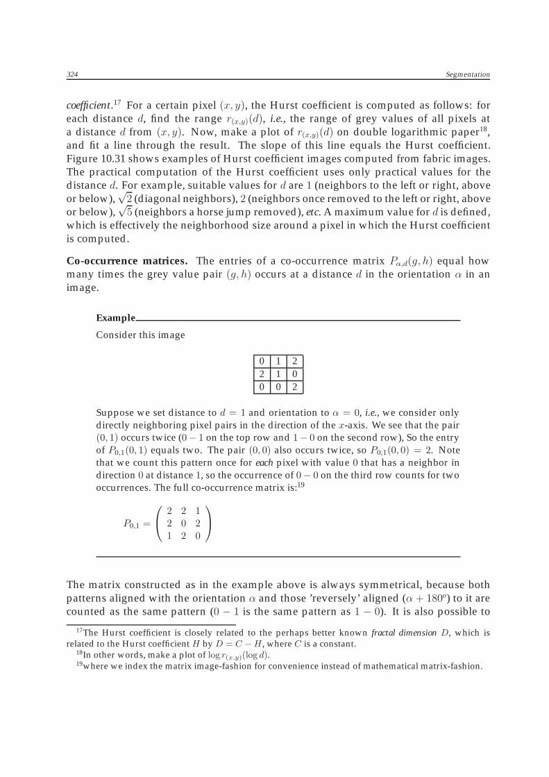
324 Segmentation
coefficient.17 For a certain pixel (x, y), the Hurst coefficient is computed as follows: foreach distance d, find the range r(x,y)(d), i.e., the range of grey values of all pixels ata distance d from (x, y). Now, make a plot of r(x,y)(d) on double logarithmic paper18,and fit a line through the result. The slope of this line equals the Hurst coefficient.Figure 10.31 shows examples of Hurst coefficient images computed from fabric images.The practical computation of the Hurst coefficient uses only practical values for thedistance d. For example, suitable values for d are 1 (neighbors to the left or right, aboveor below),
√2 (diagonal neighbors), 2 (neighbors once removed to the left or right, above
or below),√
5 (neighbors a horse jump removed), etc. A maximum value for d is defined,which is effectively the neighborhood size around a pixel in which the Hurst coefficientis computed.
Co-occurrence matrices. The entries of a co-occurrence matrix Pα,d(g, h) equal howmany times the grey value pair (g, h) occurs at a distance d in the orientation α in animage.
Example
Consider this image
0 1 22 1 00 0 2
Suppose we set distance to d = 1 and orientation to α = 0, i.e., we consider onlydirectly neighboring pixel pairs in the direction of the x-axis. We see that the pair(0, 1) occurs twice (0− 1 on the top row and 1− 0 on the second row), So the entryof P0,1(0, 1) equals two. The pair (0, 0) also occurs twice, so P0,1(0, 0) = 2. Notethat we count this pattern once for each pixel with value 0 that has a neighbor indirection 0 at distance 1, so the occurrence of 0− 0 on the third row counts for twooccurrences. The full co-occurrence matrix is:19
P0,1 =
⎛⎝ 2 2 1
2 0 21 2 0
⎞⎠
The matrix constructed as in the example above is always symmetrical, because bothpatterns aligned with the orientation α and those ’reversely’ aligned (α + 180o) to it arecounted as the same pattern (0 − 1 is the same pattern as 1 − 0). It is also possible to
17The Hurst coefficient is closely related to the perhaps better known fractal dimension D, which isrelated to the Hurst coefficient H by D = C −H , where C is a constant.
18In other words, make a plot of log r(x,y)(log d).19where we index the matrix image-fashion for convenience instead of mathematical matrix-fashion.
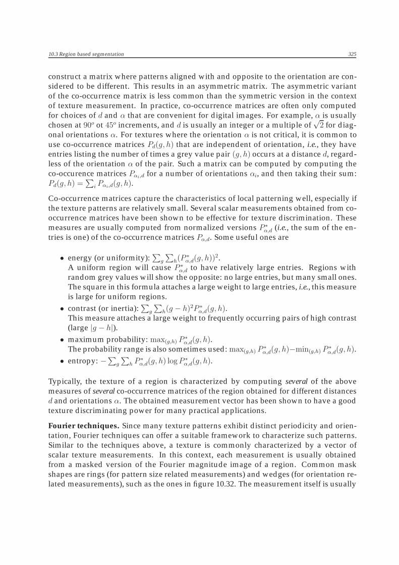
10.3 Region based segmentation 325
construct a matrix where patterns aligned with and opposite to the orientation are con-sidered to be different. This results in an asymmetric matrix. The asymmetric variantof the co-occurrence matrix is less common than the symmetric version in the contextof texture measurement. In practice, co-occurrence matrices are often only computedfor choices of d and α that are convenient for digital images. For example, α is usuallychosen at 90o ot 45o increments, and d is usually an integer or a multiple of
√2 for diag-
onal orientations α. For textures where the orientation α is not critical, it is common touse co-occurrence matrices Pd(g, h) that are independent of orientation, i.e., they haveentries listing the number of times a grey value pair (g, h) occurs at a distance d, regard-less of the orientation α of the pair. Such a matrix can be computed by computing theco-occurence matrices Pαi,d for a number of orientations αi, and then taking their sum:Pd(g, h) =
∑i Pαi,d(g, h).
Co-occurrence matrices capture the characteristics of local patterning well, especially ifthe texture patterns are relatively small. Several scalar measurements obtained from co-occurrence matrices have been shown to be effective for texture discrimination. Thesemeasures are usually computed from normalized versions P ∗
α,d (i.e., the sum of the en-tries is one) of the co-occurrence matrices Pα,d. Some useful ones are
• energy (or uniformity):∑
g
∑h(P
∗α,d(g, h))
2.A uniform region will cause P ∗
α,d to have relatively large entries. Regions withrandom grey values will show the opposite: no large entries, but many small ones.The square in this formula attaches a large weight to large entries, i.e., this measureis large for uniform regions.• contrast (or inertia):
∑g
∑h(g − h)2P ∗
α,d(g, h).This measure attaches a large weight to frequently occurring pairs of high contrast(large |g − h|).• maximum probability: max(g,h) P
∗α,d(g, h).
The probability range is also sometimes used: max(g,h) P∗α,d(g, h)−min(g,h) P
∗α,d(g, h).
• entropy: −∑g
∑h P
∗α,d(g, h) logP ∗
α,d(g, h).
Typically, the texture of a region is characterized by computing several of the abovemeasures of several co-occurrence matrices of the region obtained for different distancesd and orientations α. The obtained measurement vector has been shown to have a goodtexture discriminating power for many practical applications.
Fourier techniques. Since many texture patterns exhibit distinct periodicity and orien-tation, Fourier techniques can offer a suitable framework to characterize such patterns.Similar to the techniques above, a texture is commonly characterized by a vector ofscalar texture measurements. In this context, each measurement is usually obtainedfrom a masked version of the Fourier magnitude image of a region. Common maskshapes are rings (for pattern size related measurements) and wedges (for orientation re-lated measurements), such as the ones in figure 10.32. The measurement itself is usually

326 Segmentation
energy, i.e., the sum of squared values in the masked Fourier image, or the maximumvalue occurring in the masked Fourier image.
10.4 Clustering techniques
Clustering techniques is the collective name for methods that attempt to group togethermeasurements points (‘patterns’). For an off-topic example, let’s say we measure theweight and length of a population of rabbits. We can then plot the measurements ofeach rabbit together as shown in figure 10.33. When looking at the figure, it will be clearthat three clusters can be identified –there are very likely three types of rabbit in thepopulation. The object of clustering techniques is to identify such clusters in data. Therelation to segmentation will be clear; when viewing the rabbit plot as an image, themost intuitive segmentation would be to divide the image into segments equal to thethree clusters and the background.
Clustering techniques are often formulated for data of arbitrary dimension (not just twoas in our rabbit example), but many clustering methods can readily be applied to two-or three-dimensional images. The images best suited for applying clustering techniquesto are those similar in appearance to the rabbit plot, i.e., of a very sparse nature, the darkpixels forming quasi-coherent clouds.
The rabbit data consists of a list of pairs of measurements. This data representation isthe most natural for clustering techniques. If we wish to apply clustering to a binaryimage, we therefore use a similar representation: each pixel with value one is includedin a data list of coordinate pairs. For grey-valued images there may not be a naturalconversion to a list of data points. For some types of grey-valued images, it is possibleto consider the grey value as the number of data points measured at a certain location.
Example
This binary image:
0 1 00 1 10 0 1
can be represented as a set of data points by listing the coordinates of the ‘one’pixels:
{(1, 0), (1, 1), (2, 1), (2, 2)}.
The following grey valued image can similarly be represented by listing all coor-dinates a number of times equal to the grey value:
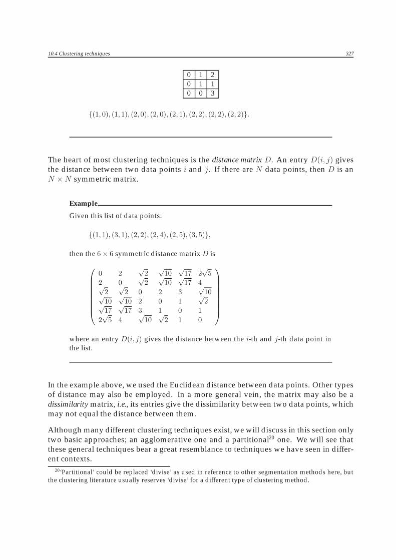
10.4 Clustering techniques 327
0 1 20 1 10 0 3
{(1, 0), (1, 1), (2, 0), (2, 0), (2, 1), (2, 2), (2, 2), (2, 2)}.
The heart of most clustering techniques is the distance matrix D. An entry D(i, j) givesthe distance between two data points i and j. If there are N data points, then D is anN ×N symmetric matrix.
Example
Given this list of data points:
{(1, 1), (3, 1), (2, 2), (2, 4), (2, 5), (3, 5)},
then the 6× 6 symmetric distance matrix D is
⎛⎜⎜⎜⎜⎜⎜⎜⎝
0 2√
2√
10√
17 2√
52 0
√2√
10√
17 4√2√
2 0 2 3√
10√10√
10 2 0 1√
2√17√
17 3 1 0 12√
5 4√
10√
2 1 0
⎞⎟⎟⎟⎟⎟⎟⎟⎠
where an entry D(i, j) gives the distance between the i-th and j-th data point inthe list.
In the example above, we used the Euclidean distance between data points. Other typesof distance may also be employed. In a more general vein, the matrix may also be adissimilarity matrix, i.e., its entries give the dissimilarity between two data points, whichmay not equal the distance between them.
Although many different clustering techniques exist, we will discuss in this section onlytwo basic approaches; an agglomerative one and a partitional20 one. We will see thatthese general techniques bear a great resemblance to techniques we have seen in differ-ent contexts.
20‘Partitional’ could be replaced ‘divise’ as used in reference to other segmentation methods here, butthe clustering literature usually reserves ‘divise’ for a different type of clustering method.
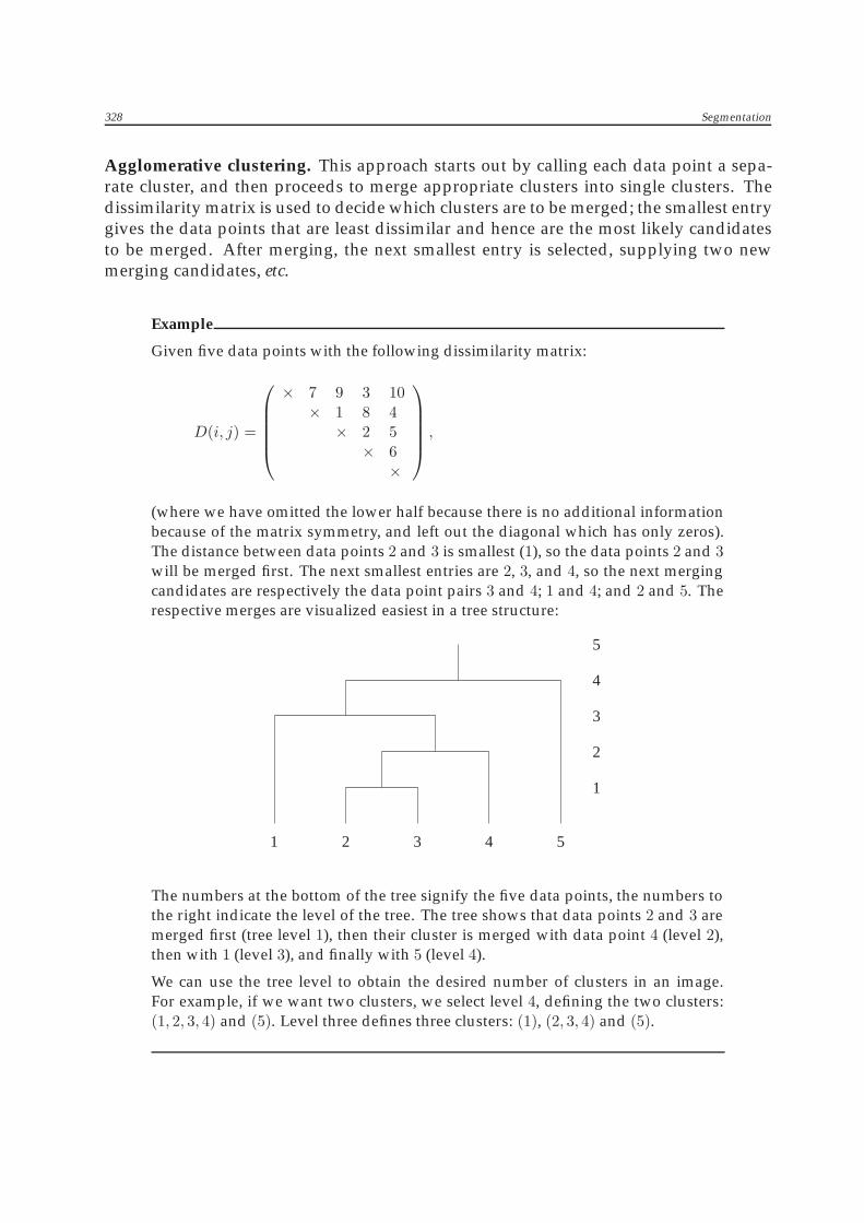
328 Segmentation
Agglomerative clustering. This approach starts out by calling each data point a sepa-rate cluster, and then proceeds to merge appropriate clusters into single clusters. Thedissimilarity matrix is used to decide which clusters are to be merged; the smallest entrygives the data points that are least dissimilar and hence are the most likely candidatesto be merged. After merging, the next smallest entry is selected, supplying two newmerging candidates, etc.
Example
Given five data points with the following dissimilarity matrix:
D(i, j) =
⎛⎜⎜⎜⎜⎝× 7 9 3 10× 1 8 4× 2 5× 6×
⎞⎟⎟⎟⎟⎠ ,
(where we have omitted the lower half because there is no additional informationbecause of the matrix symmetry, and left out the diagonal which has only zeros).The distance between data points 2 and 3 is smallest (1), so the data points 2 and 3will be merged first. The next smallest entries are 2, 3, and 4, so the next mergingcandidates are respectively the data point pairs 3 and 4; 1 and 4; and 2 and 5. Therespective merges are visualized easiest in a tree structure:
1
1
2
2
3
3
4
4
5
5
The numbers at the bottom of the tree signify the five data points, the numbers tothe right indicate the level of the tree. The tree shows that data points 2 and 3 aremerged first (tree level 1), then their cluster is merged with data point 4 (level 2),then with 1 (level 3), and finally with 5 (level 4).
We can use the tree level to obtain the desired number of clusters in an image.For example, if we want two clusters, we select level 4, defining the two clusters:(1, 2, 3, 4) and (5). Level three defines three clusters: (1), (2, 3, 4) and (5).
10.4 Clustering techniques 329
The type of tree used in the above example is usually called a dendrogram. An algorithmto perform the above described clustering is:
Algorithm:Given n data points and a dissimilarity matrix D:
1. Initialize by defining each data point to be a separate cluster. Set an iterationcounter c = 0.
2. Select the smallest entry in D: D(a, b) = min(i,j)
D(i, j).
3. Merge the clusters a and b.
4. Update D:
(a) Update row b and column b by settingD(k, b) = min{D(k, a), D(k, b)} and D(b, k) = D(k, b), both for all possible k,k = a, k = b.
(b) Delete row a and column a
5. Increase c by one, and go to step 2 if c < n.
This algorithm will merge clusters if there are member data points that are closest con-sidering all data point pairs. A variation on this algorithm is to merge two clusters ifthe largest distance between its member data points is the smallest when consideringall clusters. This can be achieved by a simple modification of the above algorithm: the‘min’ in the update step 4 must be replaced by ‘max’.
Partitional clustering. The most frequently used form of partitional clustering is todivide the data points into clusters in such a way that the total distance of data pointsto their respective cluster centers is minimal. An algorithm to achieve this is called K-means clustering, and we have already seen this algorithm in a one-dimensional guiseearlier in this chapter.
Algorithm: K-means clusteringThis algorithm minimizes the total distance of data points to the cluster center of thecluster they are assigned to. Note that it does not require the actual computation ofdistances.
1. Select the number of desired clusters k. Arbitrarily (or better: intelligently) placethe k cluster centers at different initial locations in the image.
2. Assign each data point to the cluster whose center is closest.
3. Recompute the cluster centers; the cluster center should be at the average coor-dinates (center of gravity) of the data points that make up the cluster.
330 Segmentation
4. Go to step 2 until no more changes occur or a maximum number of iterations isreached.
A drawback of this algorithm is that the number of desired clusters needs to be set be-forehand. An addition to the above algorithm is therefore to embed it into an outer loopthat modifies the number of clusters, or, more precisely, removes irrelevant clusters, andsplits existing clusters where appropriate. After this modification, the entire new algo-rithm is iterated until stable. A criterion for removal of a cluster is when the number ofcontained data points falls below a set threshold. When this happens, the data pointsare probably outliers and can usually be safely ignored in the rest of the process. Acriterion for splitting a cluster can be when a distance can be found of a contained datapoint to the cluster center that is relatively large compared to the average distance ofthe data point to all cluster centers. The splitting can then be implemented by settingthis data point to be the center of a new cluster.
In a manner similar to pyramid-tree segmentation, the algorithm can be extended to beprobabilistic, i.e., data points can belong to several clusters simultaneously, or –moreprecisely– are assigned a probability distribution giving the probabilities of the datapoint belonging to particular clusters. This probabilistic variant is usually called fuzzyclustering.
10.5 Matching
If we want to locate an object in an image, and we have available an example of what itshould look like (a template), we can find this object by matching the template to variousimage locations until we have found the object. For an example, see figure 10.34. Themost straightforward way of determining whether a template ‘fits’ would be to place thetemplate at a certain image location, and see whether the grey values of the templateand the underlying image image grey values all match. However, because there willgenerally be some differences between the image and template values because of noiseand other artifacts, this is not a very practical method. More useful is a quantitativemeasure of fit such as
M1(p, q) =
M−1∑x=0
N−1∑y=0
(g(x, y)− f(x+ p, y + q))2 ,
where f is the image, g the M × N template, and the variables p and q determine thelocation of the template in the image, see figure 10.35. This measure will be small if

10.5 Matching 331
the template is similar to the part of the image under investigation; then all grey valuedifferences g(x, y)− f(x+ p, y+ q) are small and the sum M1 will be small. The locationof optimal template fit is found by minimizing M1 to p and q.
Besides the squared form M1, another often used measure is M2, which uses the actualgrey value differences instead of their squares:
M2(p, q) =M−1∑x=0
N−1∑y=0
|g(x, y)− f(x+ p, y + q)|.
M2 puts less weight on relatively large grey value differences than M1. But perhaps themost commonly used measure is the cross correlation M3, which is defined by
M3(p, q) =M−1∑x=0
N−1∑y=0
g(x, y)f(x+ p, y + q).
The maximum of M3 with respect to p and q is assumed to indicate the location in theimage where the template fits best. There is a strong relation between the measures M1
and M3, which is most obvious if we extend the sums in the measure M1 to the entireimage f (and pad the template g with zeros); then the measure M3 appears literallybetween constants if we expand the square:
M∗1 (p, q) =
dx−1∑x=0
dy−1∑y=0
(f(x, y)− g(x− p, y − q))2
=∑∑
f 2(x, y)︸ ︷︷ ︸constant
−2∑∑
f(x, y)g(x− p, y − q)︸ ︷︷ ︸=M3
+∑∑
g2(x− p, y − q)︸ ︷︷ ︸constant
where dx and dy are the dimensions of the image f .
-normalized cc
-example
40x40 around optimal position,optimal pos obviously at image center

332 Segmentation
-other measures
-other transforms
-patt recogn
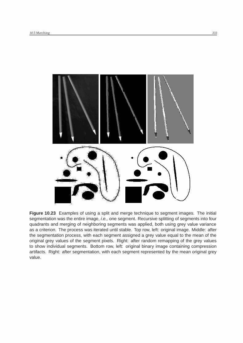
10.5 Matching 333
Figure 10.23 Examples of using a split and merge technique to segment images. The initialsegmentation was the entire image, i.e., one segment. Recursive splitting of segments into fourquadrants and merging of neighboring segments was applied, both using grey value varianceas a criterion. The process was iterated until stable. Top row, left: original image. Middle: afterthe segmentation process, with each segment assigned a grey value equal to the mean of theoriginal grey values of the segment pixels. Right: after random remapping of the grey valuesto show individual segments. Bottom row, left: original binary image containing compressionartifacts. Right: after segmentation, with each segment represented by the mean original greyvalue.
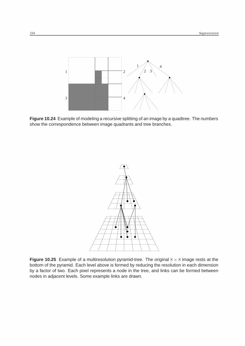
334 Segmentation
1 2
3 4
12 3
4
Figure 10.24 Example of modeling a recursive splitting of an image by a quadtree. The numbersshow the correspondence between image quadrants and tree branches.
Figure 10.25 Example of a multiresolution pyramid-tree. The original 8 × 8 image rests at thebottom of the pyramid. Each level above is formed by reducing the resolution in each dimensionby a factor of two. Each pixel represents a node in the tree, and links can be formed betweennodes in adjacent levels. Some example links are drawn.
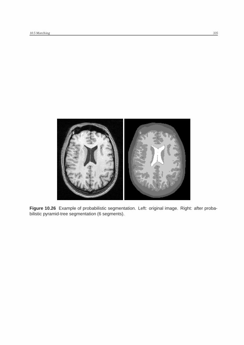
10.5 Matching 335
Figure 10.26 Example of probabilistic segmentation. Left: original image. Right: after proba-bilistic pyramid-tree segmentation (6 segments).
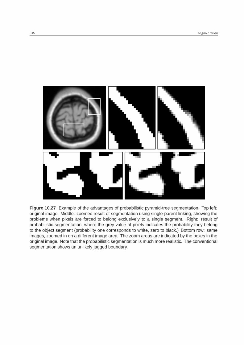
336 Segmentation
Figure 10.27 Example of the advantages of probabilistic pyramid-tree segmentation. Top left:original image. Middle: zoomed result of segmentation using single-parent linking, showing theproblems when pixels are forced to belong exclusively to a single segment. Right: result ofprobabilistic segmentation, where the grey value of pixels indicates the probability they belongto the object segment (probability one corresponds to white, zero to black.) Bottom row: sameimages, zoomed in on a different image area. The zoom areas are indicated by the boxes in theoriginal image. Note that the probabilistic segmentation is much more realistic. The conventionalsegmentation shows an unlikely jagged boundary.
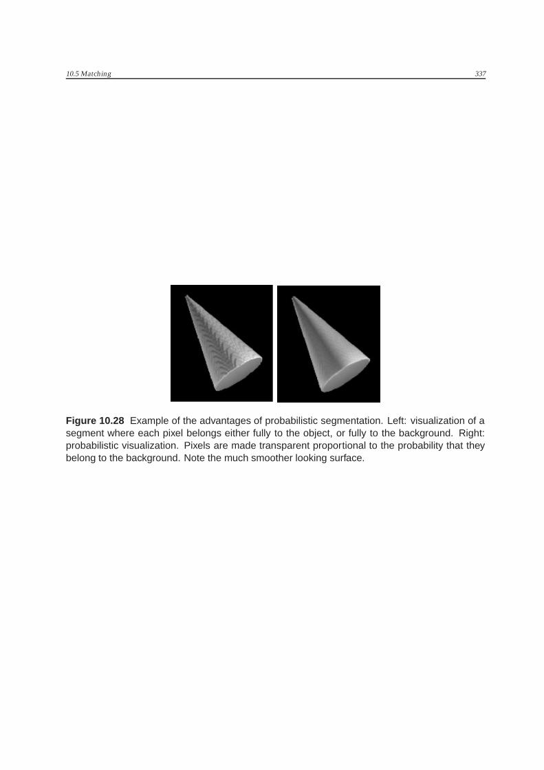
10.5 Matching 337
Figure 10.28 Example of the advantages of probabilistic segmentation. Left: visualization of asegment where each pixel belongs either fully to the object, or fully to the background. Right:probabilistic visualization. Pixels are made transparent proportional to the probability that theybelong to the background. Note the much smoother looking surface.

338 Segmentation
Figure 10.29 Examples of various kinds of texture.

10.5 Matching 339
-6 -4 -2 2 4 6
0.75
0.8
0.85
0.9
0.95
-6 -4 -2 2 4 6
0.825
0.85
0.875
0.9
0.925
0.95
0.975
-30 -20 -10 10 20 30
0.7
0.75
0.8
0.85
0.9
0.95
Figure 10.30 Plots of the autocorrelation coefficient, as a function of x-translation. The re-gion used was a 42 × 1 rectangular window. Left: autocorrelation of the window contain-ing the values {1, 2, 3, 4, 3, 2, 1, 2, 3, 4, 3, 2, 1, 2, 3, 4, 3, 2, 1, 2, 3, 4, 3, 2, 1, 2, 3, 4, 3, 2, 1, 2, 3, 4, 3, 2,-1, 2, 3, 4, 3, 2, 1, 2, 3, 4, 3, 2}, i.e., containing a pattern of length 6. Note that the peaks ofthe correlation function occur at a distance of 6 pixels. Middle: using the same window,but with added noise: {1, 5, 5, 4, 4, 6, 2, 4, 6, 7, 3, 2, 2, 2, 5, 7, 5, 2, 5, 2, 7, 7, 6, 2, 3, 3, 7, 6, 6, 6, 5, 2, 6,-7, 5, 6, 4, 3, 5, 6, 5, 5, 2, 3, 6, 7, 6, 4}. Note that the peaks of the function still occur at a six pixelinterval. Right: autocorrelation function of a window containing random values. The symme-try of all three plots is caused by using padding with the window itself to obtain unknown pixelvalues.
Figure 10.31 Hurst coefficients for two types of fabric. Left: original 120 × 120 images. Right:Hurst coefficient computed using a neighborhood of size 15. The white border stems from thefact that only neighborhoods that fit inside the image boundary were used.
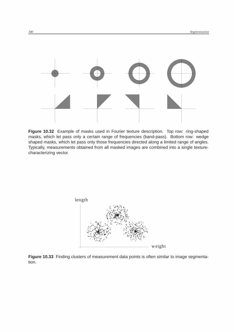
340 Segmentation
Figure 10.32 Example of masks used in Fourier texture description. Top row: ring-shapedmasks, which let pass only a certain range of frequencies (band-pass). Bottom row: wedgeshaped masks, which let pass only those frequencies directed along a limited range of angles.Typically, measurements obtained from all masked images are combined into a single texture-characterizing vector.
length
weight
Figure 10.33 Finding clusters of measurement data points is often similar to image segmenta-tion.
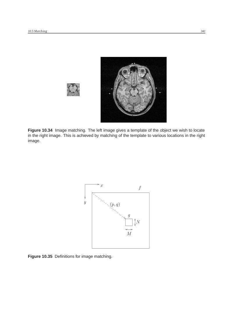
10.5 Matching 341
Figure 10.34 Image matching. The left image gives a template of the object we wish to locatein the right image. This is achieved by matching of the template to various locations in the rightimage.
x
y(p, q)
M
N
f
g
Figure 10.35 Definitions for image matching.