chapter 10 neutron stars and pulsars -...

Chapter 10

Neutron stars and pulsars

Neutron stars are relevant to our discussion of general relativity

on two levels.

• They are of considerable intrinsic interest because their

quantitative description requires solution of the Einstein

equations in the presence of matter.

• In addition, they also explain the existence of pulsars and

these in turn provide the most stringent observational tests

of general relativity.

337

338 CHAPTER 10. NEUTRON STARS AND PULSARS

10.1 The Oppenheimer–Volkov Equations

Neutron stars have an average density of order 1014−1015 g cm−3.

• This produces gravitational fields that are of moderate strength

by general relativity standards (enormous by Earth standards).

• Escape velocity at the surface is around 13c− 1

2c.

• Thus a general relativistic treatment is necessary for their correct

description.

• Unlike the vacuum Schwarzschild solution, we must now deal

with mass distributions and a finite stress–energy tensor.

• We shall, however, simplify by assuming a static, spherically

symmetric configuration for the matter.

• Boundary condition: With these assumptions we may assume

the solution outside the neutron star to correspond to the Schwarzschild

solution, so the interior solution must match Schwarzschild at

the surface.

Thus, we consider the general solution of the Einstein equations

for the gravitational field produced by

• a static, spherical mass distribution that

• matches to the exterior (Schwarzschild) solution at the

surface of the spherical mass distribution.

10.1. THE OPPENHEIMER–VOLKOV EQUATIONS 339

• The matter inside the star is a perfect fluid, with a stress energy

tensor given

Tµν = (ε +P)uµuν +Pδ

µν ,

where for later convenience we’ve written tensors in mixed form.

• Spherical symmetry, with a line element of the general form

ds2 =−eσ(r)dt2+ eλ (r)dr2+ r2dθ 2+ r2 sin2 θdϕ2,

implying non-vanishing metric components

g00(r) =−eσ(r) g11(r) = eλ (r) g22(r) = r2 g33(r,θ) = r2 sin2 θ .

Must match smoothly to the Schwarzschild metric at the surface.

• Assumed in equilibrium, so σ(r) and λ (r) are functions only of

r and not of t, and the 4-velocity has no space components:

uµ = (e−σ/2,0,0,0) = (g−1/2

00 ,0,0,0).

Inserting these 4-velocity components, the stress–energy tensor

takes the diagonal form

Tµν = (ε +P)uµuν +Pδ

µν =

−ε 0 0 0

0 P 0 0

0 0 P 0

0 0 0 P


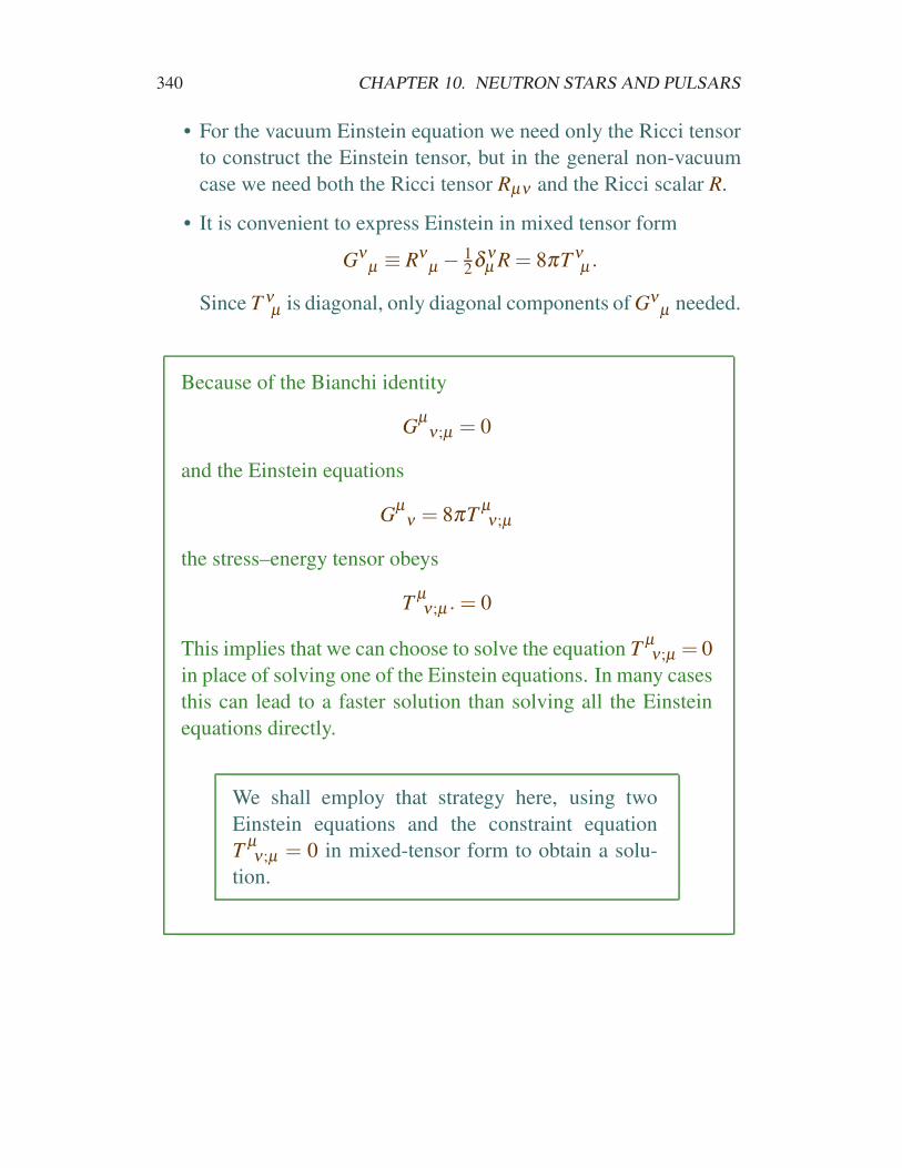
• For the vacuum Einstein equation we need only the Ricci tensor

to construct the Einstein tensor, but in the general non-vacuum

case we need both the Ricci tensor Rµν and the Ricci scalar R.

• It is convenient to express Einstein in mixed tensor form

Gνµ ≡ Rν

µ −12δ ν

µ R = 8πT νµ .

Since T νµ is diagonal, only diagonal components of Gν

µ needed.

Because of the Bianchi identity

Gµ

ν ;µ = 0

and the Einstein equations

Gµ

ν = 8πTµν ;µ

the stress–energy tensor obeys

Tµν ;µ .= 0

This implies that we can choose to solve the equation Tµν ;µ = 0

in place of solving one of the Einstein equations. In many cases

this can lead to a faster solution than solving all the Einstein

equations directly.

We shall employ that strategy here, using two

Einstein equations and the constraint equation

Tµν ;µ = 0 in mixed-tensor form to obtain a solu-

tion.


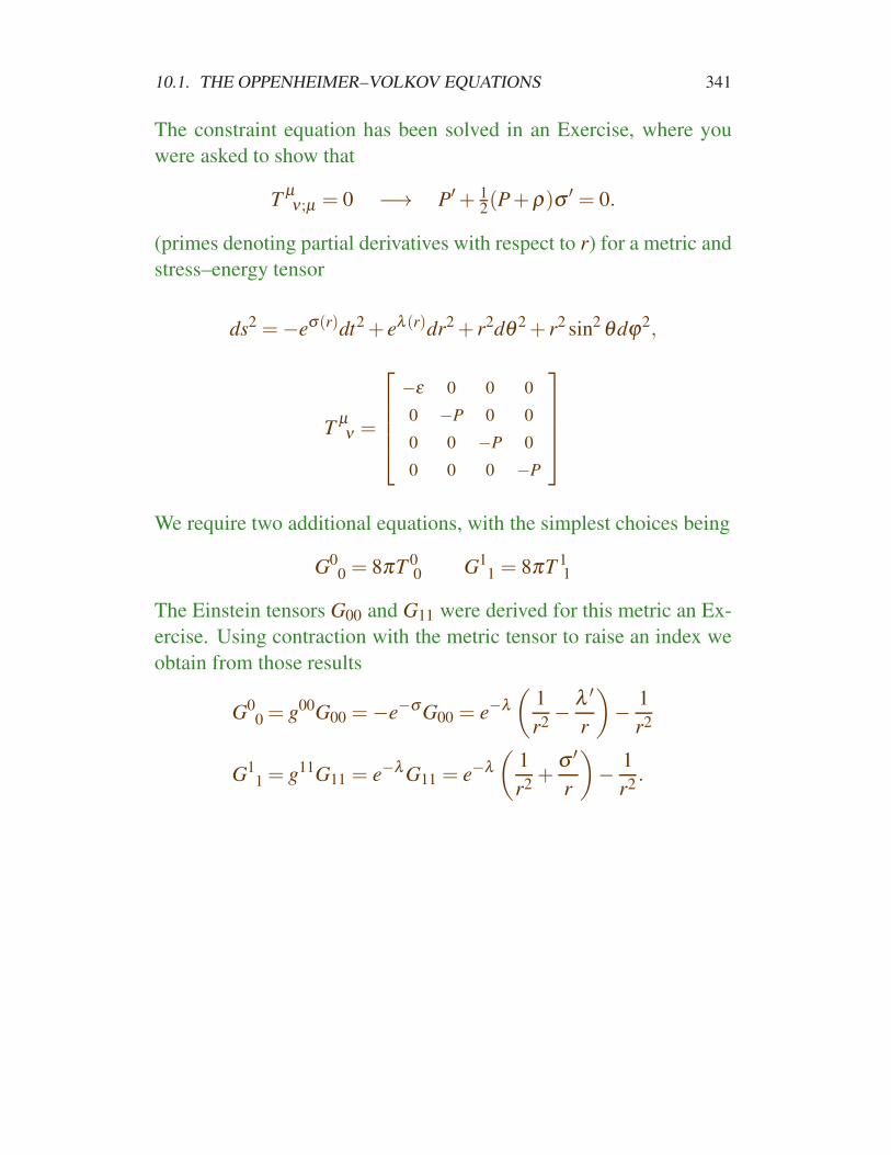
The constraint equation has been solved in an Exercise, where you

were asked to show that

Tµν ;µ = 0 −→ P′+ 1

2(P+ρ)σ ′ = 0.

(primes denoting partial derivatives with respect to r) for a metric and

stress–energy tensor

ds2 =−eσ(r)dt2+ eλ (r)dr2+ r2dθ 2+ r2 sin2 θdϕ2,

Tµν =

−ε 0 0 0

0 −P 0 0

0 0 −P 0

0 0 0 −P

We require two additional equations, with the simplest choices being

G00 = 8πT 0

0 G11 = 8πT 1

1

The Einstein tensors G00 and G11 were derived for this metric an Ex-

ercise. Using contraction with the metric tensor to raise an index we

obtain from those results

G00 = g00G00 =−e−σ G00 = e−λ

(1

r2−

λ ′

r

)

−1

r2

G11 = g11G11 = e−λ G11 = e−λ

(1

r2+

σ ′

r

)

−1

r2.


From the preceding equations we find then that we must solve

−e−λ

(1

r2−

λ ′

r

)

+1

r2= 8πε(r)

e−λ

(1

r2−

σ ′

r

)

−1

r2= 8πP(r)

P′+ 12(P+ρ)σ ′ = 0.

To proceed we note that the first Einstein equation may be rewritten

as

G00 =

1

r2

d

dr

[

r(

1− e−λ)]

=2

r2

dm

dr= 8πε,

where we have defined a new parameter

2m(r)≡ r(1− e−λ).

At this point m(r) is only a reparameterization of the metric

coefficient eλ since, upon multiplying by eλ ,

eλ =r

r−2m(r)=

(

1−2m(r)

r

)−1

,

but m(r) will be interpreted below as the total mass–energy

enclosed within the radius r. With this interpretation we note

that eλ is of the Schwarzschild form for r outside the spherical

mass distribution of the star.


from the first Einstein equation

G00 =

2

r2

dm

dr= 8πε → dm = 4πr2εdr,

and thus

m(r) = 4π

∫ r

0ε(r)r2 dr,

with an integration constant m(0) = 0 chosen on physical grounds.

Now consider the second Einstein equation

e−λ

(1

r2−

σ ′

r

)

−1

r2= 8πP(r)

Solving it for σ ′ = dσ/dr gives

dσ

dr= eλ

(

8πrP(r)+1

r

)

−1

r,

and substitution of

eλ =r

r−2m(r)

leads todσ

dr=

8πr3P(r)+2m(r)

r(r−2m(r)).

Therefore the preceding two equations may be used to define

the metric coefficients eσ and eλ in terms of the parameter m(r)and the pressure P(r).


Finally, we may combine

P′+ 12(P+ρ)σ ′ = 0 and

dσ

dr=

8πr3P(r)+2m(r)

r(r−2m(r))

to give

dP

dr=−

(P(r)+ ε(r))(4πr3P(r)+m(r))

r(r−2m(r)).

Collecting our results, we have obtained the Oppenheimer–

Volkov equations for the structure of a static, spherical, gravi-

tating perfect fluid

dP

dr=

(P(r)+ ε(r))(m(r)+4πr3P(r)

)

r2

(

1−2m(r)

r

) ,

m(r) = 4π

∫ r

0ε(r)r2 dr

where m(r) is the total mass contained within a radius r


dP

dr=

(P(r)+ ε(r))(m(r)+4πr3P(r)

)

r2

(

1−2m(r)

r

) ,

m(r) = 4π

∫ r

0ε(r)r2 dr

• Solution of these equations requires specification of an equation

of state that relates the density to the pressure.

• They may then be integrated from the origin outward with initial

conditions m(r = 0) = 0 and an arbitrary choice for the central

density ε(r = 0) until the pressure P(r) becomes zero.

• This defines the surface of the star r = R, with the mass of the

star given by m(R).

• For a given equation of state each choice of ε(0) will give a

unique R and m(R) when the equations are integrated.

• This defines a family of stars characterized by a specific equation

of state and the value of a single parameter (the central density,

or a quantity related to it like central pressure).


These equations represent the general relativistic (covariant) descrip-

tion of hydrostatic equilibrium for a spherical, gravitating perfect

fluid.

• The condition of hydrostatic equilibrium was built into the solu-

tion through the assumption

uµ = (e−σ/2,0,0,0) = (g−1/200 ,0,0,0).

which constrains the fluid to be static since the 4-velocity has no

non-zero space components.

• They reduce to the Newtonian description of hydrostatic equi-

librium in the limit of weak gravitational fields

However, the Oppenheimer–Volkov equations imply significant devi-

ations from the Newtonian description in strong gravitational fields

such as those for neutron stars. To see this clearly, a little algebra

allows us to rewrite them in the form (Exercise)

4πr2dP(r) =−m(r)dm(r)

r2

×

(

1+P(r)

ε(r)

)(

1+4πr3P(r)

m(r)

)(

1−2m(r)

r

)−1

dm(r) = 4πr2ε(r)dr.

These equations may be interpreted in the following way:


4πr2dP(r)︸︷︷︸

Force acting on shell

=−m(r)dm(r)

r2︸︷︷︸

Newtonian

×

1+P(r)

ε(r)︸︷︷︸

GR

1+4πr3P(r)

m(r)︸︷︷︸

GR

1−2m(r)

r︸︷︷︸

GR

−1

dM(r) = 4πr2ε(r)dr︸︷︷︸

Mass–energy of shell

.

• The second equation gives the mass–energy of a shell lying be-

tween radii r and r+dr.

• The left side of the first equation is the net force acting outward

on this shell.

• The first factor on the right side of the first equation is the attrac-

tive Newtonian gravity acting on the shell because of the mass

interior to it.


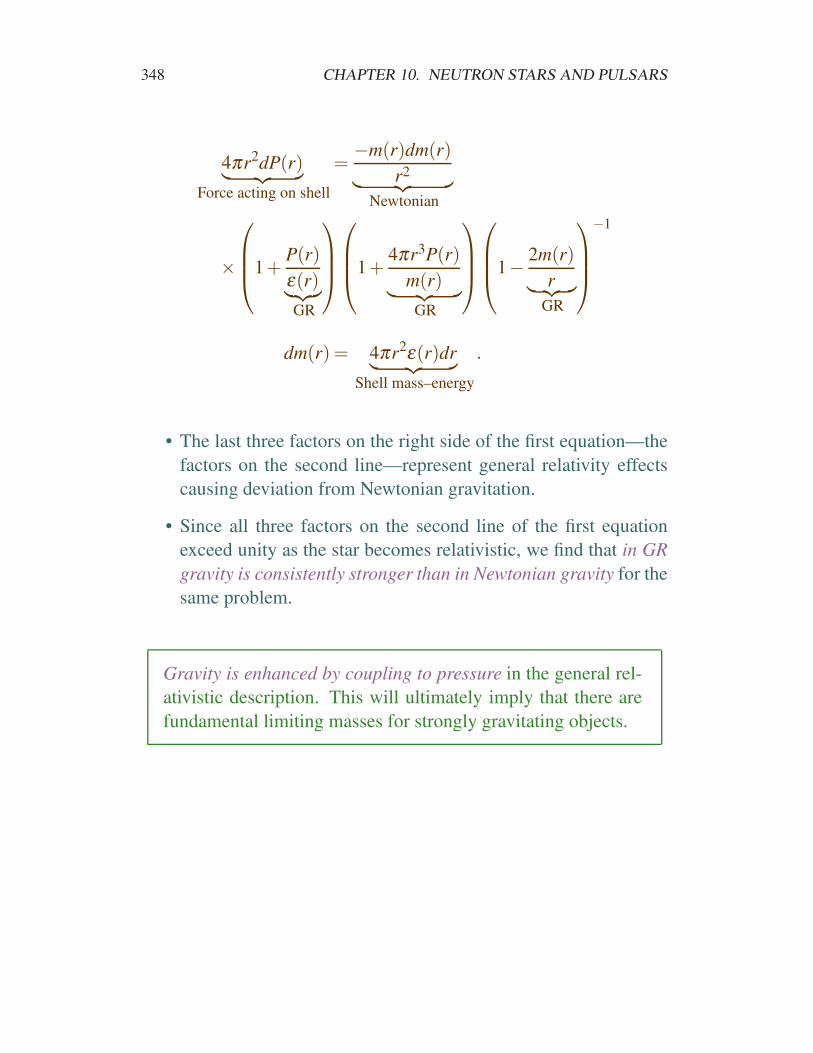
4πr2dP(r)︸︷︷︸

Force acting on shell

=−m(r)dm(r)

r2︸︷︷︸

Newtonian

×

1+P(r)

ε(r)︸︷︷︸

GR

1+4πr3P(r)

m(r)︸︷︷︸

GR

1−2m(r)

r︸︷︷︸

GR

−1

dm(r) = 4πr2ε(r)dr︸︷︷︸

Shell mass–energy

.

• The last three factors on the right side of the first equation—the

factors on the second line—represent general relativity effects

causing deviation from Newtonian gravitation.

• Since all three factors on the second line of the first equation

exceed unity as the star becomes relativistic, we find that in GR

gravity is consistently stronger than in Newtonian gravity for the

same problem.

Gravity is enhanced by coupling to pressure in the general rel-

ativistic description. This will ultimately imply that there are

fundamental limiting masses for strongly gravitating objects.

10.2. INTERPRETATION OF THE MASS PARAMETER 349

10.2 Interpretation of the Mass Parameter

The parameter m(r) entering the Oppenheimer–Volkov equations has

been interpreted provisionally as the total mass–energy enclosed within

a radius r. Let us now justify this interpretation.

• Outside a star of radius R, the mass function m(r) becomes equal

to m(R), which is the mass that would be detected through Ke-

pler’s law for the orbital motion if the star were a component of

a well-separated binary system.

• In the Newtonian limit it is clear from

m(r) = 4π

∫ r

0ε(r)r2 dr,

that m(r) can be unambiguously interpreted as the mass con-

tained within the radius r.

• For relativistic stars m(r) may be consistently split into a con-

tribution from a rest mass m0(r), an internal energy U(r), and a

gravitational energy Ω(r),

m(r) = m0(r)+U(r)+Ω(r),

as we now demonstrate.

• Formally we can split the energy density ε into a contribution

from the rest mass and one from internal energy,

ε = µ0n+(ε −µ0n),

where the first term is the total rest mass of n particles of average

mass µ0 and the second term in parentheses is the contribution

of internal energy.


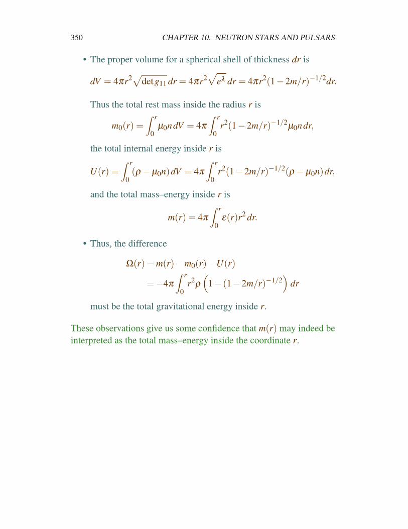
• The proper volume for a spherical shell of thickness dr is

dV = 4πr2√

detg11 dr = 4πr2√

eλ dr = 4πr2(1−2m/r)−1/2dr.

Thus the total rest mass inside the radius r is

m0(r) =∫ r

0µ0ndV = 4π

∫ r

0r2(1−2m/r)−1/2µ0ndr,

the total internal energy inside r is

U(r) =∫ r

0(ρ −µ0n)dV = 4π

∫ r

0r2(1−2m/r)−1/2(ρ −µ0n)dr,

and the total mass–energy inside r is

m(r) = 4π

∫ r

0ε(r)r2 dr.

• Thus, the difference

Ω(r) = m(r)−m0(r)−U(r)

=−4π

∫ r

0r2ρ

(

1− (1−2m/r)−1/2)

dr

must be the total gravitational energy inside r.

These observations give us some confidence that m(r) may indeed be

interpreted as the total mass–energy inside the coordinate r.

10.2. INTERPRETATION OF THE MASS PARAMETER 351

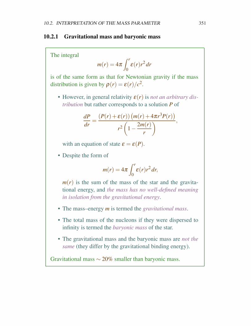
10.2.1 Gravitational mass and baryonic mass

The integral

m(r) = 4π

∫ r

0ε(r)r2 dr

is of the same form as that for Newtonian gravity if the mass

distribution is given by ρ(r) = ε(r)/c2.

• However, in general relativity ε(r) is not an arbitrary dis-

tribution but rather corresponds to a solution P of

dP

dr=

(P(r)+ ε(r))(m(r)+4πr3P(r)

)

r2

(

1−2m(r)

r

) ,

with an equation of state ε = ε(P).

• Despite the form of

m(r) = 4π

∫ r

0ε(r)r2 dr,

m(r) is the sum of the mass of the star and the gravita-

tional energy, and the mass has no well-defined meaning

in isolation from the gravitational energy.

• The mass–energy m is termed the gravitational mass.

• The total mass of the nucleons if they were dispersed to

infinity is termed the baryonic mass of the star.

• The gravitational mass and the baryonic mass are not the

same (they differ by the gravitational binding energy).

Gravitational mass ∼ 20% smaller than baryonic mass.


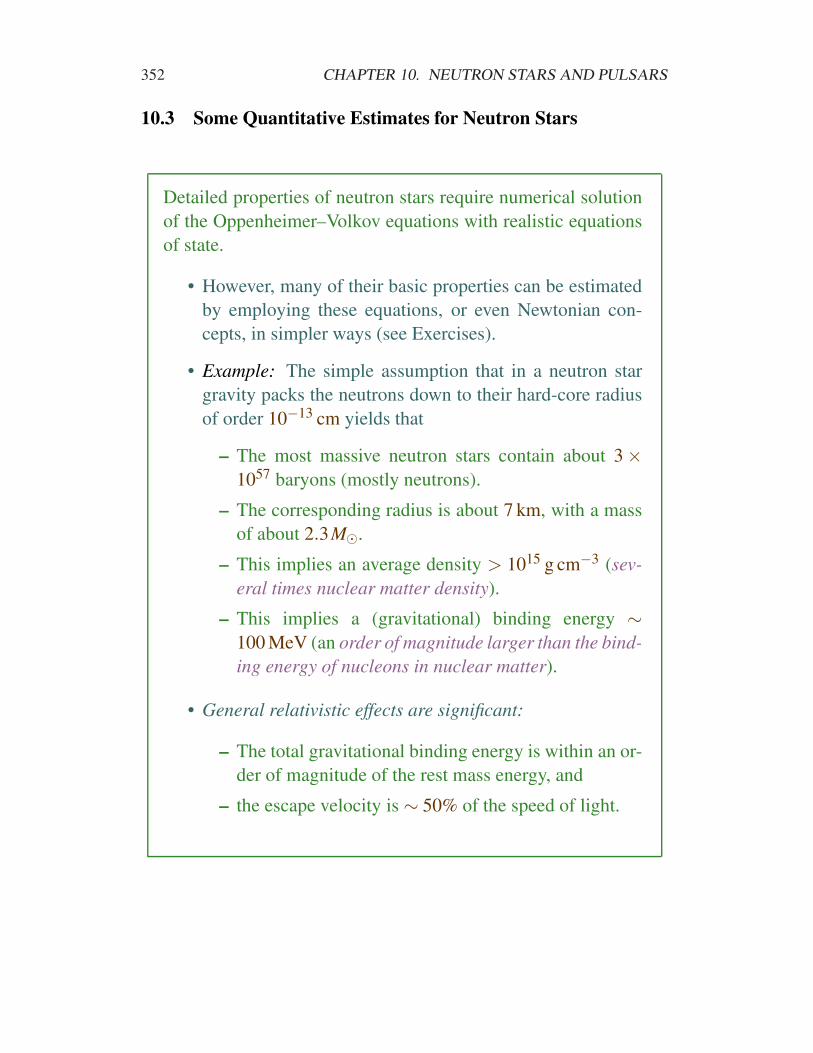
10.3 Some Quantitative Estimates for Neutron Stars

Detailed properties of neutron stars require numerical solution

of the Oppenheimer–Volkov equations with realistic equations

of state.

• However, many of their basic properties can be estimated

by employing these equations, or even Newtonian con-

cepts, in simpler ways (see Exercises).

• Example: The simple assumption that in a neutron star

gravity packs the neutrons down to their hard-core radius

of order 10−13 cm yields that

– The most massive neutron stars contain about 3 ×

1057 baryons (mostly neutrons).

– The corresponding radius is about 7 km, with a mass

of about 2.3M⊙.

– This implies an average density > 1015 g cm−3 (sev-

eral times nuclear matter density).

– This implies a (gravitational) binding energy ∼

100 MeV (an order of magnitude larger than the bind-

ing energy of nucleons in nuclear matter).

• General relativistic effects are significant:

– The total gravitational binding energy is within an or-

der of magnitude of the rest mass energy, and

– the escape velocity is ∼ 50% of the speed of light.

10.3. SOME QUANTITATIVE ESTIMATES FOR NEUTRON STARS 353

Although general relativity is important for the overall proper-

ties of neutron stars, over a microscopic scale characteristic of

nuclear and other sub-atomic interactions the metric is essen-

tially constant.

• Thus the microphysics (nuclear and elementary particle

interactions) of the neutron star can be described by quan-

tum mechanics implemented in flat spacetime (special rel-

ativistic quantum field theory).

• For neutron stars it is possible to decouple gravity (which

governs the overall structure) from quantum mechanics

(which governs the microscopic properties)


10.4 The Binary Pulsar

The Binary Pulsar PSR 1913+16 (also known as the Hulse–

Taylor pulsar) was discovered using the Arecibo 305 meter ra-

dio antenna.

• It is about 5 kpc away, near the boundary of the constella-

tions Aquila and Sagitta.

• This pulsar rotates 17 times a second, giving a pulsation

period of 59 milliseconds.

• It is in a binary system with another neutron star (not a

pulsar), with a 7.75 hour period.

• The precise repetition frequency of the pulsar means that it

is basically a very high quality clock orbiting in a binary

system that feels very strong, time-varying gravitational

effects.

−→ Precise tests of general relativity

10.4. THE BINARY PULSAR 355

Puls

es/s

econd

Time (hours)

Radia

l velo

city

(km

/s)

16.93

16.94

16.95

16.96

0

-100

-200

-300PeriastronPeriastron

Receding

Approaching

0 2 4 6 7.75

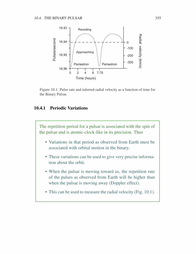
Figure 10.1: Pulse rate and inferred radial velocity as a function of time for

the Binary Pulsar.

10.4.1 Periodic Variations

The repetition period for a pulsar is associated with the spin of

the pulsar and is atomic-clock-like in its precision. Thus

• Variations in that period as observed from Earth must be

associated with orbital motion in the binary.

• These variations can be used to give very precise informa-

tion about the orbit.

• When the pulsar is moving toward us, the repetition rate

of the pulses as observed from Earth will be higher than

when the pulsar is moving away (Doppler effect).

• This can be used to measure the radial velocity (Fig. 10.1).


The pulse arrival times vary as the pulsar moves through its

orbit

• It takes three seconds longer for the pulses to arrive from

the far side of the orbit than from the near side.

• From this, the Binary Pulsar orbit can be inferred to be

about a million kilometers (three light seconds) further

away from Earth when on the far side of its orbit than

when on the near side.

10.4. THE BINARY PULSAR 357

Periastron

Apastron

1.1 R

4.8 R

Orbital plane

tilted by 45o

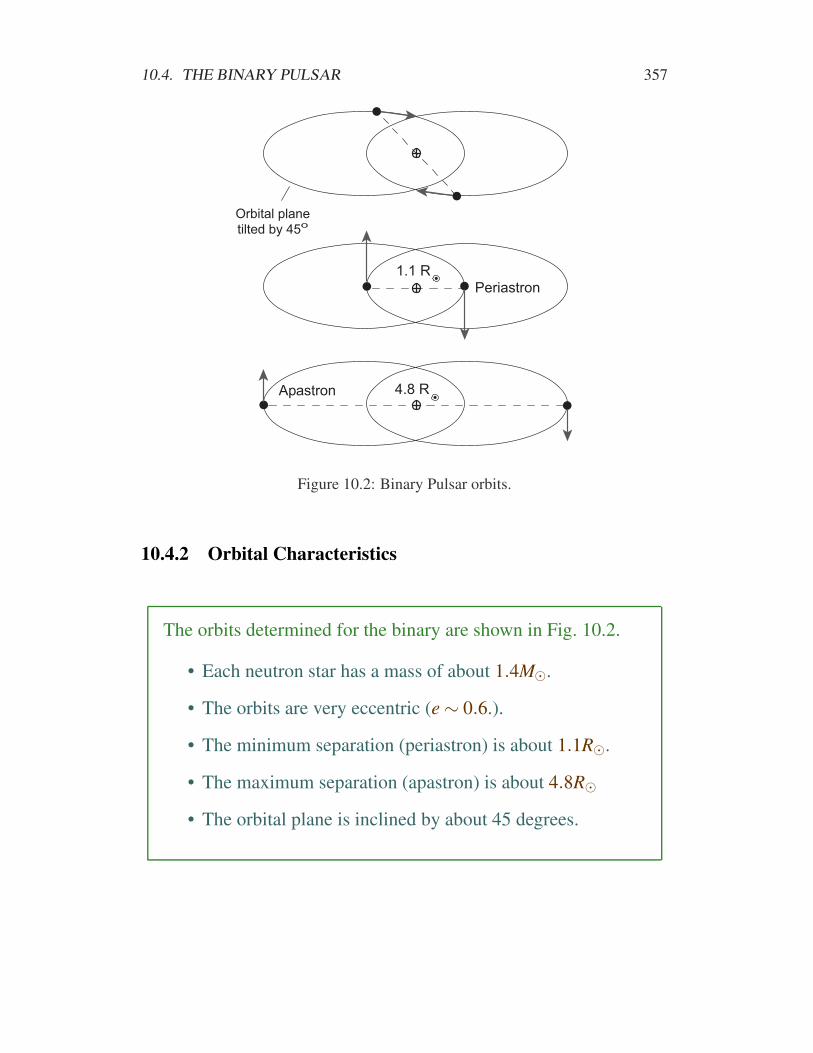
Figure 10.2: Binary Pulsar orbits.

10.4.2 Orbital Characteristics

The orbits determined for the binary are shown in Fig. 10.2.

• Each neutron star has a mass of about 1.4M⊙.

• The orbits are very eccentric (e ∼ 0.6.).

• The minimum separation (periastron) is about 1.1R⊙.

• The maximum separation (apastron) is about 4.8R⊙

• The orbital plane is inclined by about 45 degrees.


Centero f mass

Orb i t 3

Orb i t 2

Orb i t 1

P1

P2

P3

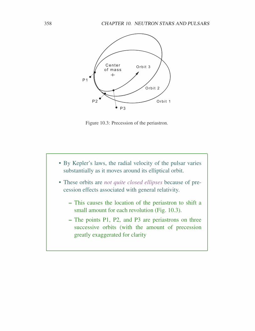
Figure 10.3: Precession of the periastron.

• By Kepler’s laws, the radial velocity of the pulsar varies

substantially as it moves around its elliptical orbit.

• These orbits are not quite closed ellipses because of pre-

cession effects associated with general relativity.

– This causes the location of the periastron to shift a

small amount for each revolution (Fig. 10.3).

– The points P1, P2, and P3 are periastrons on three

successive orbits (with the amount of precession

greatly exaggerated for clarity

10.5. PRECISION TESTS OF GENERAL RELATIVITY 359

10.5 Precision Tests of General Relativity

The discovery and study of the Binary Pulsar was of such fun-

damental importance that Taylor and Hulse were awarded the

Nobel Prize in Physics for their work

• This was the only Nobel ever given for relativity before

the 2017 prize for discovery of gravitational waves.

• Chief among the reasons for this importance is that the

Binary Pulsar provided the most stringent tests of general

relativity available before the discovery of the Double Pul-

sar.


Centero f mass

Orb i t 3

Orb i t 2

Orb i t 1

P1

P2

P3

10.5.1 Precession of Orbits

Because spacetime is warped by the gravitational field in the vicinity

of the pulsar, the orbit will precess with time.

• This is the same effect as the precession of the perihelion of

Mercury, but it is much larger for the present case.

• The Binary Pulsar’s periastron advances by 4.2 degrees per year,

in accord with the predictions of general relativity.

• In a single day the orbit of the Binary Pulsar advances by as

much as the orbit of Mercury advances in a century!

10.5.2 Time Dilation

• When the binary pulsar is near periastron, gravity is stronger and

its velocity is higher and time should run slower.

• Conversely, near apastron the field is weaker and the velocity

lower, so time should run faster.

• It does both, in the amount predicted by GR.

10.5. PRECISION TESTS OF GENERAL RELATIVITY 361

Companion star

250 million years

Size of

Sun

Now

Shrink

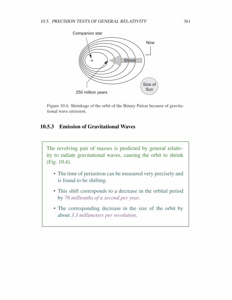
Figure 10.4: Shrinkage of the orbit of the Binary Pulsar because of gravita-

tional wave emission.

10.5.3 Emission of Gravitational Waves

The revolving pair of masses is predicted by general relativ-

ity to radiate gravitational waves, causing the orbit to shrink

(Fig. 10.4).

• The time of periastron can be measured very precisely and

is found to be shifting.

• This shift corresponds to a decrease in the orbital period

by 76 millionths of a second per year.

• The corresponding decrease in the size of the orbit by

about 3.3 millimeters per revolution.


1975 1980 1985 1990 1995 2000 2005-40

-35

-30

-25

-20

-15

-10

-5

0

Year

General relativity

Cu

mu

lative

pe

ria

str

on

sh

ift (s

)

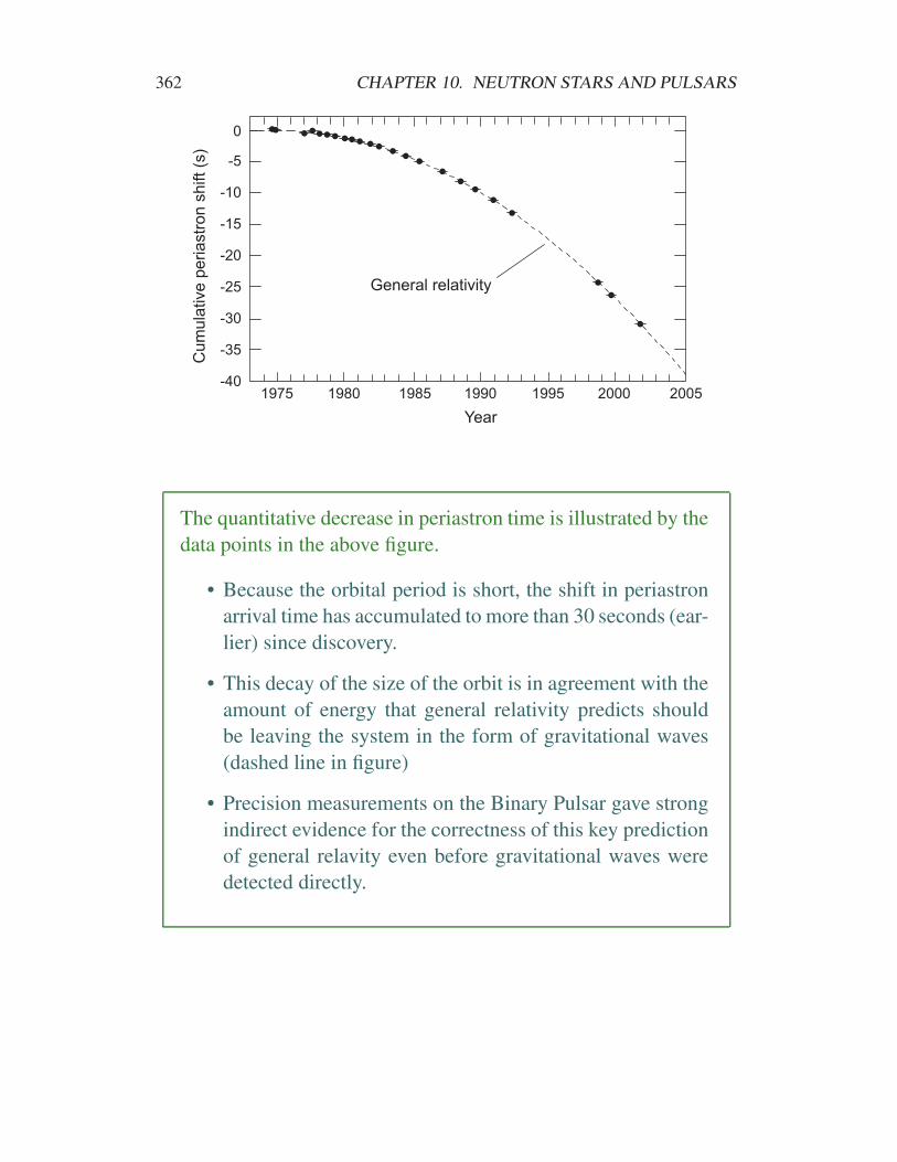
The quantitative decrease in periastron time is illustrated by the

data points in the above figure.

• Because the orbital period is short, the shift in periastron

arrival time has accumulated to more than 30 seconds (ear-

lier) since discovery.

• This decay of the size of the orbit is in agreement with the

amount of energy that general relativity predicts should

be leaving the system in the form of gravitational waves

(dashed line in figure)

• Precision measurements on the Binary Pulsar gave strong

indirect evidence for the correctness of this key prediction

of general relavity even before gravitational waves were

detected directly.

10.6. ORIGIN AND FATE OF THE BINARY PULSAR 363

10.6 Origin and Fate of the Binary Pulsar

Formation of a neutron star binary is not easy. One of two

things must happen

• A binary must form with two stars massive enough to be-

come supernovae and produce neutron stars, and the neu-

tron stars thus formed must remain bound to each other

through the two supernova explosions.

• The neutron star binary must result from gravitational cap-

ture of one neutron star by another.

These are improbable events, but not impossible, and the exis-

tence of the Binary Pulsar (and several similar systems) demon-

strates empirically that mechanisms exist for it to happen.


Once a neutron star binary is formed its orbital motion radi-

ates energy as gravitational waves, the orbits must shrink, and

eventually the two neutron stars must merge.

• Because of the gravitational wave radiation and the cor-

responding shrinkage of the Binary Pulsar orbit (3.3 mil-

limeters per revolution), merger is predicted in about 300

million years.

• The sum of the masses of the two neutron stars is likely

above the critical mass to form a black hole. Therefore,the

probable fate of the Binary Pulsar is merger and collapse

to a rotating (Kerr) black hole.

• As two neutron stars in a binary approach each other they

will revolve faster (Kepler’s third law).

• This will cause them to emit gravitational radiation more

rapidly, which will in turn cause the orbit to shrink even

faster.

• Thus, near the end the merger of two neutron stars will

proceed rapidly in a positive-feedback runaway and will

emit very strong gravitational waves that may be de-

tectable with current-generation gravitational wave detec-

tors.

These considerations are valid for any binary, not just the Bi-

nary Pulsar, but the gravitational wave effects are much more

pronounced for binaries involving highly compact objects.

10.7. THE DOUBLE PULSAR 365

PSR J0737-3039B To Earth

PSR J0737-3039A

Double

Pulsar

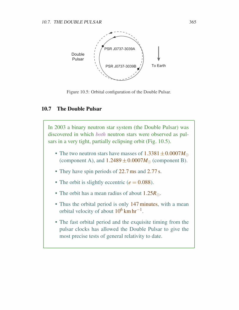
Figure 10.5: Orbital configuration of the Double Pulsar.

10.7 The Double Pulsar

In 2003 a binary neutron star system (the Double Pulsar) was

discovered in which both neutron stars were observed as pul-

sars in a very tight, partially eclipsing orbit (Fig. 10.5).

• The two neutron stars have masses of 1.3381±0.0007M⊙

(component A), and 1.2489±0.0007M⊙ (component B).

• They have spin periods of 22.7 ms and 2.77 s.

• The orbit is slightly eccentric (e = 0.088).

• The orbit has a mean radius of about 1.25R⊙.

• Thus the orbital period is only 147 minutes, with a mean

orbital velocity of about 106 km hr−1.

• The fast orbital period and the exquisite timing from the

pulsar clocks has allowed the Double Pulsar to give the

most precise tests of general relativity to date.

chapter 10 neutron stars and pulsars -...

Documents