Chapter 1

Stress and Strain

1.1 Introduction

The opto-structural analyst is concerned with stress and deflection fromexternally applied loads, such as those occurring during mounting of optics, andinternal loads, such as those initiated by gravity or acceleration. Additionally,the analyst is concerned with temperature change, which causes deflection andoften causes stress. For cryogenic and high-temperature extremes, such valuesare obviously crucial; for more benign environments, temperature, loads, andself-weight deflection are still an issue, since we are concerned with fractional-wavelength-of-light changes. Accordingly, this initial chapter provides thebasics of structural analysis, which lay the foundation for the chapters to follow.

1.2 Hooke’s Law

Before diving into the structural analysis methods required for high-acuityoptical systems, it is useful to review the origins of this analysis. While basicand advanced theories and principles of strength of materials and structuralanalysis have filled volumes, we review here the basis on which everythingelse follows. We review, therefore, the simple relation developed by RobertHooke1 in 1660, when he wrote ut tensio sic vis,2 which literally means, “as theextension, so the force.” This expression simply states that force, or load, isdirectly proportional to deflection for any system that can be treated as amechanical spring, including elastic bodies, as long as such deflection is small.Simply stated,

F ¼ kx, (1.1)

where F is the applied force, x is the resulting deflection, and k is a spring, orstiffness, constant. In this theory, the spring is fully restored to its originallength upon removal of the load.

A logical extension to Hooke’s law relates stress to strain in a similarfashion. Consider a bar of length L and a cross-sectional area A under an axialload P, as shown in Fig. 1.1. Here, we define stress s as

1

s ¼ PA: (1.2)

Note that this is simply a definition; stress has the units of force divided byarea [MN/m2 (MPa)], or pounds per square inch (psi).

The load in Fig. 1.1 and the resulting stress are considered to be tensilewhen the object is stretched and are compressive when it is shortened. Tensileand compressive stresses are called direct stresses and act normal to the cross-sectional surface.

Since stress is directly proportional to force divided by area, and strain ε(a dimensionless quantity) is related to deflection as

ε ¼ xL, (1.3)

we can now rewrite Hooke’s law as

s ¼ Eε, (1.4)

where E is a material stiffness constant; for a solid isotropic material undera unidirectional axial load, E is an inherent property of the material, calledits modulus of elasticity, and often referred to as elastic modulus, tensilemodulus, or Young’s modulus. The modulus of elasticity has the same units asstress (psi) since strain is dimensionless.

Substituting Eq. (1.4) into Eq. (1.2), we now readily compute the axialdeflection of the bar of Fig. 1.1 as

x ¼ PLAE

: (1.5)

While this formulation is quite simplified, computation of stress for 3D solidswith loads in multiple directions will be more complex. To illustrate this, andfor the sake of completeness, while force is a vector (it has magnitude anddirection), i.e., a first-order tensor, stress is a second-order tensor, which is amultidirectional quantity, and follows a different set of rules than the simplelaws of vector addition. Further, for anisotropic materials, the stiffness matrixrelating stress to strain will, in general, consist of a fourth-order tensor and21 independent terms, with Hooke’s law taking the form of

Figure 1.1 Direct tension force application to a one-dimensional (1D) element. Stress isdefined as force divided by area and acts normal to the surface of the cross-section.

2 Chapter 1

sij ¼X3k¼1

X3i¼1

Eijklεkl, (1.6)

where subscripts i, j take on values of 1, 2, or 3. Fortunately, in this text, wewill not make use of such advanced analyses and will need only to discussstress and strain in two dimensions, enabling more simplified, yet accurate,analyses. In the case of isotropic loading of 3D solids, the stiffness matrix isreduced to only two quantities, E and G, the latter of which is defined as theshear modulus, or modulus of rigidity. The shear modulus G is related to theelastic modulus E as

G ¼ E2ð1þ nÞ , (1.7)

where n is the ratio of lateral contraction to axial elongation under axial loadand varies between 0 and 0.5 for most common materials. Values of zero arecommon for cork, for example, and values near 0.5 are common for rubbers,which are essentially incompressible. Another way of saying this is that for amaterial such as rubber, its volume will be constant under load, while itsvolume is ever increasing as Poisson’s ratio is lowered toward zero.(Theoretical values of Poisson’s ratio can be as low as �1, as achieved incertain materials, and are well beyond the scope of this text).

In two dimensions,

Ex ¼ðsx � nsyÞ

E, (1.7a)

Ey ¼ðsy � nsxÞ

E: (1.7b)

Thus, for the purposes of this text, these equations are most useful andpreclude the need for unwieldy, 3D constituency matrices. The introduction ofthe 2D effect gives rise to the additional form of Hooke’s law relating to shearstress t, given as

t ¼ Gl, (1.8)

where l is the (dimensionless) shear strain angle.Shear stresses act in the plane of the cross-sectional surface. For shear

load force V, as depicted in Fig. 1.2, we find the average shear stress as

t ¼ VA: (1.9)

3Stress and Strain

Substituting Eq. (1.8) into Eq. (1.9), we now readily compute the sheardeflection (ignoring beam bending for the moment) of the bar of Fig. 1.2 as

y ¼ VLAG

: (1.10)

1.3 Beyond Tension, Compression, and Shear

Thus far, we have applied Hooke’s law in the three translational directions:axial (x, tension/compression) and lateral (y, z, shear). There are also threerotational directions upon which bending and twist moments may act,completing the six possible degrees of freedom. Bending occurs when amoment is applied about either of the orthogonal lateral (y, z) axes, whiletwisting occurs when a moment [in units of inch-pounds (in.-lb)] is appliedabout the axial (x) axis. Figure 1.3 depicts these additional degrees offreedom. Again, in these cases, we can use Hooke’s law to determine stressesand strains, and, therefore, deformation.

1.3.1 Bending stress

It is worthwhile to illustrate Hooke’s law for the case of bending. Consider abeam under pure bending (constant, uniform moment), as shown in Fig. 1.4.

Figure 1.2 Direct shear force application without bending to a 1D element. Stress isdefined as force divided by area and acts in the plane of the surface cross-section.

Figure 1.3 1D beam element under bending (about the z and y axes) and twist moments(about the x axis) in rotational degrees of freedom. Bending produces normal stress, whiletwist produces shear stress.

4 Chapter 1

The top (concave) surface is shortened, and the bottom (convex) surface iselongated. Somewhere in the middle there is no length change; this is theneutral axis of the beam. Since adjacent planes rotate by an amount du, thearc length s at the neutral surface is given as

s ¼ dx ¼ Rdu, (1.11)

where R is the radius of curvature of the beam.Away from the neutral surface, the beam fibers elongate or shorten by an

amount ydu, and since the original fiber length was dx, the strain is givensimply as

ε ¼ � ydudx

¼ � yR, (1.12)

where a positive sign indicates tension, and a negative sign indicatescompression. We can now apply Hooke’s law (Eq. 1.4) and readily compute

s ¼ EyR

: (1.13)

These stresses acting over the elemental area give rise to forces thatproduce the resultant moment. Since there is no net force, from equilibrium itis realized that

ER

ZydA ¼ 0, (1.14)

Figure 1.4 Diagram of bending stress showing section curves with radius R under momentloading. Surface a–a shortens, while surface b–b lengthens relative to neutral surface c–c.

5Stress and Strain

which implies that the neutral axis is at the centroid of the cross-section. Thenet moment M is the sum of the force distance products, or

M ¼Z

ysdA ¼ ER

Zy2dA, (1.15)

where the integral is called the area moment of inertia I of the cross-section,with dimensions of length to the fourth power. Thus, we have

1R

¼ MEI

, (1.16)

and substitution of Eq. (1.16) into Hooke’s law [Eq. (1.13)] yields

s ¼ MyI

: (1.17)

The largest value occurs as either tension or compression at the extremefibers. Denoting the extreme fiber position as y ¼ c, the maximum stress is

s ¼ McI

: (1.18)

1.3.1.1 Combined normal stress

If a tensile or compressive axial load exists with a moment load, Eq. (1.18) isadded to Eq. (1.2) (normal stresses acting in the same direction can be added):

s ¼ PAþMc

I: (1.19)

It has been said that this equation is 90% of structural engineering; this isan obvious exaggeration, but the equation is, arguably, one of the mostcommonly used equations in structural analysis.

1.3.2 Bending deflection

For a beam of length L, it is a simple matter to compute the bendingdeformation y using the approximate parabolic relation

y ¼ L2

8R: (1.20)

From Eq. (1.16), for a beam in pure bending,

y ¼ ML2

8EI: (1.21)

6 Chapter 1

Most commonly, the moment is not uniform, as is the case when trans-verse shear loads are introduced. Here, the curvature will vary along the beam,and differential equations—well documented in basic strength of materialsliterature3 but not detailed here—give rise to deformations dependent on loadand boundary conditions. For the simple case of the cantilever beam shown inFig. 1.5, the deformation under end load P is

y ¼ PL3

3EI, (1.22)

and for the simply supported beam of Fig. 1.6,

y ¼ PL3

48EI: (1.23)

Of course, deflection can be accompanied by rotation, which is the slopeof the deflection curve. Table 1.1 shows the typical cases of beam deflectionand rotation for various loading and support boundary conditions. Supportboundary conditions can be free, meaning no restraint, and free to translateand rotate; roller, meaning free to translate in one direction but restrained inthe other, and free to rotate; pinned, meaning restrained in translation in bothdirections but free to rotate; fixed, meaning restrained in both translation androtation; and guided, meaning not free to rotate but providing for freedom totranslate in one direction.

1.3.3 Shear stress due to bending

Section 1.1 presents the shear stress due to direct shear. When shear isaccompanied by bending, the maximum shear stress occurs at the neutral axisand varies to zero at the free boundaries. In this case, the “average” shear

Figure 1.6 Simply supported beam bending under the central load will deflect at the centeraccording to Eq. (1.23). There is no translation at the end points, which are allowed to rotate.

Figure 1.5 Cantilever beam bending under the end load will deflect at end B according toEq. (1.22). There is no rotation or translation at fixed end A.

7Stress and Strain

stress of Eq. (1.9) is exceeded at the neutral zone. The maximum shear stresscan be computed as

t ¼ VQIt

, (1.24)

where Q is the area moment about the neutral zone and is given as

Q ¼Z

ydA, (1.24a)

Table 1.1 Moment, deflection, and rotation for various loading and boundary conditions.

Max.Moment

Max.Deflection

End Rotation

A B

Cantilever end load PL PL3/3EI 0 PL2/2EI

Cantilever end moment M ML2/2EI 0 ML/EI

Guided cantilever end load PL/2 PL3/12EI 0 0

Cantilever uniform load WL/2 WL3/8EI 0 WL2/6EI

Propped cantilever endmoment load

M ML2/27EI 0 ML/4EI

Simple supportcentral load

PL/4 PL3/48EI PL2/16EI PL2/16EI

Simple supportend moment

M 0.0612ML2/EI ML/6EI ML/3EI

Simple supportend moment

M ML2/8EI ML/2EI ML/2EI

Simple supportuniform load

WL/8 5WL3/38EI WL2/24EI WL2/24EI

Fixed supportcentral load

WL/8 WL3/192EI 0 0

Fixed supportsuniform load

WL/12 WL3/384EI 0 0

8 Chapter 1

and t is the thickness of the cross-section at the neutral zone. Equation (1.24)can therefore be rewritten as

t ¼ kVA

, (1.25)

where

k ¼ AQIt

: (1.26)

For the case of a rectangle,

t ¼ 3V2A

, (1.26a)

and for a circular cross-section,

t ¼ 4V3A

: (1.26b)

1.3.4 Shear deflection due to bending (detrusion)

Similarly, Section 1.1 presents shear deflection of a beam due to direct shear.When shear is accompanied by bending, shear deflection (sometimes referredto as shear detrusion) depends on both the variation in shear across the beamand the value of Q. In the case of a pure cantilever, we modify Eq. (1.10) andfind that

y ¼ kVLAG

: (1.27)

For other loading and boundaries where the shear varies with beamlength, we can use energy methods to compute deflection. For example, for asimply supported beam under a concentrated central load (first row ofTable 1.1),

y ¼ kVL4AG

: (1.28)

The value of k [computed in Eq. (1.26)] assumes that, in computation of sheardeflection, the cross-section is free to warp. This is not the case for manyconditions of loading where shear changes abruptly, as in the case of thesimply supported beam with a concentrated central load. More-complexstrain energy formulation shows that, in this case for a rectangular

9Stress and Strain

cross-section, we find a modified coefficient as approximately k ¼ 6/5, andfor a circular cross-section, k ¼ 7/6.

Deflection due to shear is generally small compared to deflection due tobending unless the span is short and/or the cross-section is deep. However, forlightweight optics (Chapter 6), shear deflection does have added importance.

1.3.5 Torsion

The final degree of freedom is twist about the axial axis, or torsion. Torque T(in units of pounds) is the torsional moment producing the twist. Again,Hooke’s law applies, in this case, for shear [Eq. (1.8)]. Similar to what is donein bending (but not shown here), it is derived that torsional stress t equals

t ¼ aTtK

, (1.29)

where a is cross-section correction constant; t is the minimum thicknessdimension of the cross-section; and K, with units of length to the fourthpower, is called the torsional constant. The torsional constant equals the polarmoment of inertia J for a circular (solid or hollow) cross-section, where

J ¼ 2I : (1.30)

In this case, a ¼ 0.5 (note that t ¼ diameter), and

t ¼ TRJ

, (1.31)

where R is the cross-sectional radius.For a noncircular cross-section, the torsional constant is not the polar

moment of inertia and needs a separate calculation. For a rectangular solidcross-section,

K ¼ Bbt3, (1.32)

where b is the long-side width, and t is the short-side thickness of the section.The value of the torsional stiffness constant B is given in the plot of Fig. 1.7 asa function of the width-to-thickness ratio. Note that for thin sections, thevalue of B approaches 1/3.

The value for the torsional stress constant a is given in the plot of Fig. 1.8.Note that a approaches unity for a thin cross-section.

For hollow, thin-walled (t), closed, rectangular cross-sections,

K ¼ 4tA20

U, (1.33)

10 Chapter 1

where A0 is the area enclosed by the mean center line of the wall, and U is theperimeter of the mean centerline of the wall.

The value of a for use in Eq. (1.29) is

a ¼ 2A0

Ut, (1.34)

from which we find that

t ¼ T2A0t

: (1.35)

Figure 1.7 Torsional stiffness constant B versus width-to-thickness ratio for a rectangularcross-section. Values approach one-third for a thin cross-section.

Figure 1.8 Torsional stress constant a versus width-to-thickness ratio for a rectangularcross-section. Values approach unity for a thin cross-section.

11Stress and Strain

Note that for a hollow, circular cross-section, Eq. (1.35) reduces to

t ¼ TRJ

,

as it must.

1.3.5.1 Twist rotation

The angle of twist is similarly derived and is given as

u ¼ TLKG

, (1.36)

where, again, K is the torsional constant depending on the cross-section asdiscussed above. For thin-walled sections such as channel or U shapes, thevalue of b can be assumed to be the total developed width of the section, to thefirst order. Table 1.2 summarizes the value of K for typical cross-sections.

1.3.6 Hooke’s law summary

Some basic derivations using Hooke’s law have been presented. While thestress and displacement calculations for more-complex situations are exhaus-tive if not nearly infinite (and, again, well documented in standard engineeringtexts and handbooks), the intent here is to set the foundation for the materialthat follows only as applied to opto-structural analysis. With an understand-ing of the basics of Hooke’s law, we can better understand its more-detailedformulations.

1.4 Combining Stresses

When normal (perpendicular to the area cross-section) stresses from tension,compression, or bending exist at a point, they can be combined directly. Whenin-plane shear stresses from torsion or direct shear exist at a point, they can becombined directly. However, as indicated in Section 1.2, stress, unlike force, isnot a vector and exists in multiple orientations. Thus, when shear stresses arecombined with normal stresses at a given point, they can neither be addedalgebraically nor vector summed, as the rules of tensor addition will apply.The addition can also be formulated by considerations of equilibrium. At anyangle in a plane, the normal and shear stresses are given, respectively, as

s ¼ ðsx þ syÞ2

þ ðsx � syÞ2

cos 2u� txy sin 2u, (1.37)

t ¼ ðsx � syÞ2

sin 2uþ txy cos 2u: (1.38)

12 Chapter 1

Because these equations define the normal and shear stresses of a circle, atechnique that uses what’s called Mohr’s circle is very useful in visualizingthese stresses through their relationship to each other: At some angle, normalstress will be maximum and will occur where the shear stress is zero.

Differentiating Eq. (1.37) with respect to angle u, and setting the resultingexpression equal to zero (max-minima problem), we can find the angle of themaximum normal stress as

tan 2u ¼ 2tðsx � syÞ

: (1.39)

By substitution, the maximum normal stress is calculated as

Table 1.2 Torsional constant K for various cross-sections. Dimensions of the constant arein length to the fourth power.

Section Torsional Constant K

Solid circle pD4/32

Solid square 0.141b4

Solid rectangle (see Fig. 1.7)

Hollow square tube b3/t

Round tube pD3t/4

Open section (thin wall) 0.333 (b1þ b2)t3

13Stress and Strain

s1 ¼ðsx þ syÞ

2þ

ffiffiffiffiffiffiffiffiffiffiffiffiffiffiffiffiffiffiffiffiffiffiffiffiffiffiffiffiffiffiffiffiðsx � syÞ2

4þ t2

s(1.40)

and is called the major principal stress.The minimum stress is similarly found as

s2 ¼ðsx þ syÞ

2�

ffiffiffiffiffiffiffiffiffiffiffiffiffiffiffiffiffiffiffiffiffiffiffiffiffiffiffiffiffiffiffiffiðsx � syÞ2

4þ t2

s(1.41)

and is called the minor principal stress.The maximum shear stress will always occur 45 deg from the principal

stress angle and is calculated as

tmax ¼ðs1 � s2Þ

2: (1.42)

Note that the principal stress always equals or is greater than the appliednormal stress and is used for determining strength.

1.4.1 Brittle and ductile materials

Principal stresses are well correlated to test strength data obtained formaterials as long as they are brittle, since they generally have higher com-pressive strength than tensile strength. Brittle materials exhibit a low strainelongation to failure after the yield point is reached. With reference toFig. 1.4, note that all of what has been presented applies in the linear region ofa stress strain diagram, for which Hooke’s law applies, i.e., below the materialyield point at which it becomes nonlinear.

For ductile materials, the stresses are not conservative, and prematureyielding may result. In this case, distortion energy methods are used, resultingin a maximum-stress prediction called von Mises stress. For two dimensions,von Mises stress is given as

smax ¼ffiffiffiffiffiffiffiffiffiffiffiffiffiffiffiffiffiffiffiffiffiffiffiffiffiffiffiffiffiffiffis21 � s1s2 þ s2

2

q(1.43)

and should be used for materials that have high strain elongation beforefailure in yield. Note that the von Mises stress is an “equivalent” stress to becompared to the material yield strength and is not a true stress. Based ondistortion theory, the premise is that the material fails by distortion, or inshear, as will be shown in the following example.

14 Chapter 1

Using the von Mises criteria for the case of an object in tension (x axisonly) and shear, we find from Eqs. (1.40), (1.41), and (1.43) that

smax ¼ffiffiffiffiffiffiffiffiffiffiffiffiffiffiffiffiffiffis2x þ 3t2

q: (1.44)

Under pure shear alone,

smax ¼ffiffiffi3

pt, (1.45)

or

t ¼ smaxffiffiffi3

p ¼ 0.577smax: (1.46)

Thus, the distortion energy theory predicts that the shear strength is 0.577times the tensile strength. This relation is common for most metals and otherductile isotropic materials.

A comparison of von Mises and principal stresses for typical, common 2Dstates of stress is given in Table 1.3.

1.5 Examples for Consideration

It is useful to illustrate the principles we have just discussed with some simpleexamples. We stress the word simple because the intent of this section is todefine the basics and the basis for the material to follow. More-complexcalculations will be introduced later as needed.

Example 1. Consider a beam fixed at one end (cantilevered) and loaded at itsfree end with an axial tensile load (x axis) of P ¼ 1000 lbs and a shear Y loadof V ¼ 2000 lbs. The beam is 5 in. long with a rectangular cross-section ofdimensions ½ in. wide by 2 in. deep. It is made of aluminum with an elasticmodulus of 1.0 � 107 psi, a Poisson ratio of 0.33, and a yield strength of35,000 psi.

Compute the following:

a) the normal stress sxb) the shear stress tc) the principal stresses s1,s2d) the von Mises stress smaxe) the maximum shear stress tmaxf) the axial displacement xg) the bending deflection ybh) the shear deflection ys

15Stress and Strain

Solutions:

a) The normal stress due to the axial load [from Eq. (1.2)] is

s ¼ PA

¼ 10001

¼ 1000 psi:

The normal stress due to the shear load results from the maximumbending moment, which is M ¼ VL.

The normal bending stress [from Eq. (1.18)] is

s ¼ VLcI

¼ 6VLbh2

¼ 7500 psi:

At a particular point at the extreme fiber, we add the normal stresses.The combined normal stress is s ¼ 1000þ 7500 ¼ 8500 psi.

Table 1.3 Principal and von Mises stresses for various elemental loading types. In general,von Mises stress equals or exceeds principal stress in 2D analysis.

Principal StressVon Mises

StressMajor Minor

Uniaxialtension

1 0 1

Pure shear 1 �1 1.732

Biaxialtension

1 1 1

Tension andcompression

1 �1 1.732

Uniaxialtension and shear

1.618 �0.618 2

16 Chapter 1

b) The shear stress [from Eq. (1.26a)] is

t ¼ 3V2A

¼ 3000 psi:

c) The major principal stress [from Eq. (1.40)] is

s1 ¼sx

2þ

ffiffiffiffiffiffiffiffiffiffiffiffiffiffiffiffiffiffiffiffiffiffiffiffi�sx

2

�2þ t2

s¼ 9450 psi,

and the minor principal stress [from Eq. (1.41)] is

s2 ¼sx

2�

ffiffiffiffiffiffiffiffiffiffiffiffiffiffiffiffiffiffiffiffiffiffiffiffi�sx

2

�2þ t2

s¼ �950 psi:

d) The von Mises stress is calculated from Eq. (1.43) as

s ¼ smax ¼ffiffiffiffiffiffiffiffiffiffiffiffiffiffiffiffiffiffiffiffiffiffiffiffiffiffiffiffiffiffiffis21 � s1s2 þ s2

2

q¼ 9960 psi:

The von Mises stress is only slightly higher than the principal stress butshould be used because the material is ductile.e) The maximum shear stress is calculated from Eq. (1.42) as

tmax ¼ðs1 � s2Þ

2¼ 5200 psi:

f) The axial displacement [from Eq. (1.5)] is

x ¼ PLAE

¼ 0.0005 in:

g) The bending deflection is found from Eq. (1.22) or Table 1.1 and is

yb ¼VL3

3EI¼ 0.025 in:

h) The shear deflection [from Eq. (1.27)] is

ys ¼kVLAG

, where k ¼ 65

ys ¼ 0.0032 in:

The shear deflection can be added directly to the bending deflection. Notethat shear deflection is typically small compared to bending deflection unlessthe beam length is extremely small or the cross-section is very deep.

17Stress and Strain

Example 2. A cantilever beam having properties and dimensions identical tothose in Example 1 above is subjected to an end torsional twist of 4000 in-lb.

Compute the following:

a) the shear stressb) the major principal stressc) the von Mises stressd) the angle of twist

Solution:

a) The shear stress [from Eq. (1.29)] is given as

t ¼ Tabt2

¼ 24800 psi:

b) The major principal stress [from Eq. (1.40)] equals the shear stress:

s1 ¼ 24800 psi:

c) The von Mises stress [from Eq. (1.45)] is

smax ¼ffiffiffi3

pt ¼ 43000 psi:

Note that the von Mises stress is significantly higher than the principalstress, and, in fact, exceeds the yield strength of the material. Since thematerial is ductile, the von Mises stress should be used; if the principalstress were used, a false sense of security might result, unless the useris aware that shear strength drives the design. In the latter case, if theprincipal stress were used, the astute analyst would check both theprincipal and maximum shear stresses, and would see that shearstrength drives the design.

d) The angle of twist is computed from Eq. (1.36) as

u ¼ TLKG

¼ TLBbt3

¼ 0.066 rad ¼ 3.8 deg :

1.6 Thermal Strain and Stress

As we have seen from Hooke’s law [Eqs. (1.1) and (1.4)], when an externalforce is applied to a member, stress is produced, and that stress is alwaysaccompanied by strain. There are cases, however, where strain is appliedwithout producing stress, as occurs under temperature loading. Consider, forexample, a beam of length L that is free to expand under a temperatureexcursion DT.

18 Chapter 1

With no restraint, the beam grows an amount

y ¼ aLDT , (1.47)

where a is the effective thermal expansion coefficient of the material over thetemperature range of interest. The beam grows according to the diagram inFig. 1.9(a). The strain is

ε ¼ yL¼ aDT : (1.48)

Because this is the natural state in which the beam occurs, there is no stress.Strain without stress is called eigenstrain.

If such a beam were completely restrained from growing [as in Fig. 1.9(b)],the amount it would naturally grow is resisted by a force, which producesstress. Thus, from Eqs. (1.5) and (1.48), we have

PLAE

¼ aLDT ; therefore,

P ¼ AEaDT ,(1.49)

and, therefore,

Figure 1.9 Thermal expansion under uniform temperature soak of (a) a stress-freeunconstrained beam and (b) a fully constrained beam inducing normal stress s. (c) Thermalexpansion of a stress-free beam simply supported at both ends with a uniform, linear, front-to-back thermal gradient.

19Stress and Strain

s ¼ PA

¼ EaDT : (1.50)

This simple equation is very important (because stress developed underthermal strain when constrained will rarely exceed this amount) and serves asan upper bound for first-order calculations. Along with Eq. (1.18), Eq. (1.50)is one of the simplest and most important relationships in opto-structuralanalysis. (Chapter 4 will expand on this in two dimensions).

Note that the resisting force is independent of length, and the developedstress is independent of both length and cross-sectional area, which is nice.Note further that if a member wants to expand and is not free to do so, theforce and stress are in compression; if it wants to shrink and is not free to doso, it is in tension.

Similarly, consider a case in which a thermal gradient is applied throughthe depth of the cross-section. For a linear gradient, we have again a case ofeigenstrain if the beam is unrestrained, and it will bend without stress to theshape shown in Fig. 1.9(c). Here, the radius (of the neutral axis) is

R ¼ taDT

: (1.51)

For a positive expansion coefficient and a positive temperature change onthe top surface, the top tends to expand and bend the beam in a convexdirection. Again, if the beam is fully constrained, stress will develop with thetop surface in compression. (In thermal cases, you sometimes have to thinkbackward.) The developed stress for the fully constrained case is

s ¼ EaDT2

: (1.52)

Note again, in this case, that the stress is independent of length and cross-sectional area or bending (area moment of) inertia. This is nice. We willexpand on this in Chapter 4, where we will also discuss nonlinear gradients,which do require cross-sectional knowledge. At this point, we have simply setthe stage for the more-detailed analyses that follow.

1.6.1 Thermal hoop stress

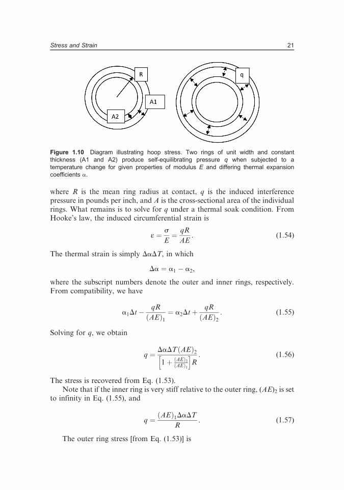
A common example of thermal stress occurs when two rings of differingcoefficients of thermal expansion (CTEs) are in contact in a thermal environ-ment, resulting in an interference that produces hoop stress in bothcomponents, as shown in Fig. 1.10. Hoop stress s is given as

s ¼ qRA

, (1.53)

20 Chapter 1

where R is the mean ring radius at contact, q is the induced interferencepressure in pounds per inch, and A is the cross-sectional area of the individualrings. What remains is to solve for q under a thermal soak condition. FromHooke’s law, the induced circumferential strain is

ε ¼ s

E¼ qR

AE: (1.54)

The thermal strain is simply DaDT, in which

Da ¼ a1 � a2,

where the subscript numbers denote the outer and inner rings, respectively.From compatibility, we have

a1Dt�qR

ðAEÞ1¼ a2Dtþ

qRðAEÞ2

: (1.55)

Solving for q, we obtain

q ¼ DaDTðAEÞ2h1þ ðAEÞ2

ðAEÞ1

iR: (1.56)

The stress is recovered from Eq. (1.53).Note that if the inner ring is very stiff relative to the outer ring, (AE)2 is set

to infinity in Eq. (1.55), and

q ¼ ðAEÞ1DaDTR

: (1.57)

The outer ring stress [from Eq. (1.53)] is

Figure 1.10 Diagram illustrating hoop stress. Two rings of unit width and constantthickness (A1 and A2) produce self-equilibrating pressure q when subjected to atemperature change for given properties of modulus E and differing thermal expansioncoefficients a.

21Stress and Strain

s ¼ qRA

¼ E1DaDT (1.58)

independent of both A and R.

1.6.1.1 Solid disk in ring

In the case of a circular, solid disk—as in an optical lens radially restrained ina cell—the induced stress is uniform throughout; i.e., its principal stress isidentical at any point. Here, the lens strain is

ε ¼ s

E¼ q

Eb, (1.59)

and the induced stress is thus

s ¼ Eε ¼ qb: (1.60)

Therefore, under thermal soak, we can modify Eq. (1.55) to yield

DaDT ¼ qRtbE1

þ qE2b

, (1.55a)

where the subscripts 1 and 2 denote the ring and disk, respectively. Hence,Eq. (1.56) can be written as

q ¼ DaDT�R

tbE1þ 1

E2b

� : (1.56a)

Note from Eq. (1.56a) that if the disk is very rigid relative to the ring, then thering stress is

s ¼ E1DaDT (1.58a)

independent of the radius, and the disk stress is

s ¼ E1tDaDTR

, (1.60a)

which is inversely proportional to the radius.Note from Eq. (1.56a) that if the ring is very rigid relative to the disk, then

the ring stress is

22 Chapter 1

s ¼ E2DaDTRt

(1.58b)

directly proportional to the radius, and the disk stress is

s ¼ E2DaDT (1.60b)

independent of the radius.

Example.We can apply these relationships to the case of a lens cell housing anoptical lens. Consider a zinc sulfide lens 1 in. deep b and 4 in. in diameterencased in a 1-in.-deep by 0.10-in.-thick t aluminum lens housing. Over a soakfrom room temperature to 150 K, compute the stress in the lens and housing.The following effective properties over the range of soak are given:

E1 ¼ 9.9� 106psi

E2 ¼ 1.08� 107psi

a1 ¼ 2.10� 10�5∕K

a2 ¼ 5.6� 10�6∕K

Since the lens is rigid relative to the housing, we find from Eq. (1.57), whereA ¼ bt, that

q ¼ ð1Þð0.1Þð9.9Þð15.4Þð143Þ2

¼ 1100 lb∕in:,

and the housing stress from Eq. (1.58) is

s ¼ ð9.9Þð15.4Þð143Þ ¼ 21800 psi:

The line pressure q on the lens is the same as that on the housing, and the lensstress, under uniform principal stress everywhere throughout, is recoveredfrom Eq. (1.60) as

s ¼ qb; therefore,

s ¼ 11001

¼ 1100 psi:

1.6.2 Ring in ring in ring

Similar to the thermal stress induced by the interference of two rings, it isuseful to review the case of thermal interference involving three rings. Thiscould occur, for example, when a thin isolation ring is housed between anoptic with a central hole and housing, or an insert is bonded to a housing. Inthis case, we need to consider the strain compatibility relationships betweenthe inner and middle rings, and between the central and outer rings. This is a

23Stress and Strain

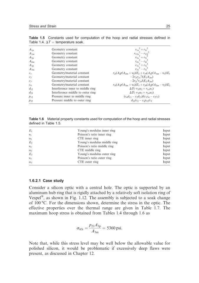
bit more complex than the two-ring problem. Figure 1.11 is a schematic of thethree-ring design, along with an equilibrium diagram. In this case, we need notlimit thickness to thin rings. Using thick-ring theory,4 and after tediouscalculations, we arrive at the individual ring stresses. We compute both radialand hoop stresses for a total of 12 stresses. (Because the inner and outer radialstresses are always zero, there are ten calculable stresses.) These stresses aregiven in Table 1.4, and the numerous constants are defined in Table 1.5. Theseconstants are readily programmable to the stress equations of Table 1.4 by useof a spreadsheet. Table 1.6 gives the material property constants used forcomputation of the hoop and radial stresses defined in Table 1.5.

When the outermost (or innermost) ring is not present and the rings arethin, the problem reduces to the simplified two-ring case of Eqs. (1.53) and(1.56) (believe it or not) with an error difference of less than 5%.

Figure 1.11 Ring-in-ring-in-ring hoop stress. Each ring has an inner and outer radius R,and each can have different modulus, thickness, and expansion characteristics. Expansionleads to self-equilibrating pressure on each surface.

Table 1.4 Tri-ring hoop and radial stresses. Subscripts 1, 2, and 3 refer to inner, middle,and outer rings, respectively; subscripts o and i refer to outer and inner surfacesrespectively; r is the radius at the specified interface; other constants are from Table 1.5.

sr1i Radial stress inner surface inner ring 0su1i Hoop stress inner surface inner ring �2p12r10

2/A1m

sr10 Radial stress outer surface inner ring –p12su10 Hoop stress outer surface inner ring –p12A1p/A1m

sr2i Radial stress inner surface middle ring –p12su2i Hoop stress inner surface middle ring (p12 A2p � 2p23r20

2)/A2m

sr20 Radial stress outer surface middle ring –p23su20 Hoop stress outer surface middle ring (2p12r2i

2� 2p23A2p)/A2m

sr3i Radial stress inner surface outer ring –p23su3i Hoop stress inner surface outer ring p23 A3p/A3m

sr30 Radial stress outer surface outer ring 0su30 Hoop stress outer surface outer ring 2p23r3i

2/A3m

24 Chapter 1

1.6.2.1 Case study

Consider a silicon optic with a central hole. The optic is supported by analuminum hub ring that is rigidly attached by a relatively soft isolation ring ofVespel®, as shown in Fig. 1.12. The assembly is subjected to a soak changeof 100 °C. For the dimensions shown, determine the stress in the optic. Theeffective properties over the thermal range are given in Table 1.7. Themaximum hoop stress is obtained from Tables 1.4 through 1.6 as

su3i ¼p23A3p

A3m¼ 5360 psi:

Note that, while this stress level may be well below the allowable value forpolished silicon, it would be problematic if excessively deep flaws werepresent, as discussed in Chapter 12.

Table 1.5 Constants used for computation of the hoop and radial stresses defined inTable 1.4. DT ¼ temperature soak.

A1p Geometry constant r1o2þ r1i

2

A1m Geometry constant r12o2� r12i

2

A2p Geometry constant r2o2þ r2i

2

A2m Geometry constant r2o2� r2i

2

A3p Geometry constant r3o2þ r3i

2

A3m Geometry constant r3o2� r3i

2

c1 Geometry/material constant r2i(A2p/A2mþ y2)/E2þ r10(A1p/A1m� y1)/E1

c2 Geometry/material constant �2r2ir2o2/(E2A2m)

c3 Geometry/material constant �2r2i2r2o/(E2A2m)

c4 Geometry/material constant r3i(A3p/A3mþ y3)/E3þ r20(A2p/A2m� y2)/E2

d12 Interference inner to middle ring DT(–r2ia2þ r1oa1)d23 Interference middle to outer ring DT(–r3ia3þ r2oa2)p12 Pressure inner to middle ring (c4d12� c2d23)/(c1c4� c2c3)p23 Pressure middle to outer ring d12/c2� c1p12/c2

Table 1.6 Material property constants used for computation of the hoop and radial stressesdefined in Table 1.5.

E1 Young’s modulus inner ring Inputy1 Poisson’s ratio inner ring Inputa1 CTE inner ring InputE2 Young’s modulus middle ring Inputy2 Poisson’s ratio middle ring Inputa2 CTE middle ring InputE3 Young’s modulus outer ring Inputy3 Poisson’s ratio outer ring Inputa3 CTE outer ring Input

25Stress and Strain

1.6.3 Nonuniform cross-section

The previous discussion of a uniform cross-section shows thermal stressindependent of cross-section or length, approaching the maximum ofEq. (1.50). However, for a nonuniform cross-section, this is not the case.

Consider, for example, the trapped 1D beam of Fig. 1.13 in which thecross-section varies and undergoes a temperature change of DT. As it becomeswarmer, the beam tends to expand stress free as

y ¼ SaiLiDT : (1.61)

Figure 1.12 Diagram of the case study setup: an aluminum hub is placed in the central holeof a silicon optic that is isolated with Vespel and undergoes a temperature soak to 100 °C.Properties and dimensions are the same as those in the example in Section 1.6.1.1.

Table 1.7 Material and dimensional properties for the case study.

Material ModulusPoisson’s Ratio CTE

Radius

Inner Outer(psi) (ppm/°C) (inch) (inch)

Aluminum 1.00Eþ07 0.33 2.15E-05 5 5.50Vespel 4.70Eþ05 0.35 4.00E-05 5.5 5.75Silicon 1.90Eþ07 0.2 2.00E-06 5.75 8.00

Figure 1.13 A fixed beam with nonunform properties subjected to temperature soak canproduce extreme stress conditions.

26 Chapter 1

The rigid wall will not let it expand and pushes back with compressive force P.Since the net deflection is zero, we have, from Hooke’s law,

P�S

�Li

A1E1

��¼ SaiLiDT (1.62)

so that

P ¼ SaiLiDT�S Li

A1E1

� ,

and

s ¼ PAi

: (1.63)

For the case shown in Fig. 1.13, we have

P ¼ ð2a1L1 þ a2L2ÞDTA1A2E1E2

ð2L1A2E2 þ L2A1E1Þ, (1.64)

and

s1 ¼PA1

¼ ð2a1L1 þ a2L2ÞDTA2E1E2

ð2L1A2E2 þ L2A1E1Þ, (1.65a)

s1 ¼PA2

¼ ð2a1L1 þ a2L2ÞDTA1E1E2

ð2L1A2E2 þ L2A1E1Þ: (1.65b)

Note that, unlike the uniform-cross-section case, stress is now dependent onboth area and length.

For the beam of Fig. 1.13, in which the modulus and CTE are constantbut the section length and the individual cross-sectional areas vary, we letb ¼ A2/A1 and g ¼ L2/L1, and substituting into Eq. (1.64), find that

s2 ¼2þ g

2bþ gEaDT : (1.66)

For equal-length sections (L1 ¼ L2), if the central cross-section is significantlysmaller than the end cross-sections, its stress approaches

s2 ¼PA2

¼ 3EaDT , (1.67)

which is in considerable excess of that for the uniform case of Eq. (1.50).

27Stress and Strain

Should the thermal stress exceed the yield point of a particular ductilematerial, the material will not necessarily fail as long as the thermal strain liesunder the material elongation capability. It will, however, be in a yieldedstate, which may require consideration for critical performance criteria. Also,if the load is compressive, buckling can occur, as discussed in the next section.

1.7 Buckling

This introductory chapter concludes with a note on critical buckling. Bucklingoccurs when a compressive axial load reaches a certain limit, causinginstability. It occurs in long, slender beams. We concentrate here on 1Dinstability, although buckling can certainly occur in plates and shells, whichare cases beyond the scope of what is presented here.

Consider the beam of Fig. 1.14 axially loaded along the x axis in com-pression. If a small load or displacement is applied laterally at the location ofthe axial load, the beam bends slightly. If the lateral load is removed, the beamreturns to its straight position. However, if the axial load is increased, nowcausing an increased moment due to the lateral eccentricity, the beam becomesunstable and does not return to its straight position when the lateral load isremoved. If the axial load increases further, the beam displacement becomesvery large, and the beam becomes unstable. This load is called the criticalbuckling load. Note that this phenomenon will only occur in compression, astensile loading will serve to straighten any eccentric lateral displacement.

We can compute the critical load by using the bending and curvaturerelations of Section 1.3 [Eq. (1.16)] and Fig. 1.4 to determine the point ofinstability. Here, we see that

Figure 1.14 Critical buckling instability occurs at a critical load in compression due to smalllateral movement. The joint at the application of the load may be free, pinned, or fixed withaxial motion allowed. The base can be pinned or fixed. The critical load depends on theseboundary conditions.

28 Chapter 1

M ¼ EIR

¼ EId2ydx2

¼ Pðd� yÞ: (1.68)

This differential equation is readily solved by calculus techniques3 to producethe critical load value at instability as

Pcr ¼p2EI4L2 : (1.69)

The solution is independent of the material strength and is only a function ofits stiffness.

While Eq. (1.69) is solved for the cantilever case, where critical value is thelowest possible, solutions are found for varying boundary conditions. If thebeam is simply supported at its ends, the critical load is

Pcr ¼p2EIL2 : (1.70)

If it is fixed at both ends, the load is

Pcr ¼4p2EIL2 , (1.71)

which is the other extreme, so we have bounded the problem.For many applications in optical structures, buckling needs to be

investigated as it may drive the design, even if stress values are below thoseallowable. We will see an example of this in Chapter 3.

References

1. R. Hooke, Lectures of Spring, Martyn, London (1678).2. R. Hooke, “A Latin (alphabetical) anagram, ceiiinosssttuv,” originally

stated in 1660 and published 18 years later.3. S. Timoshenko and D. Young, Strength of Materials, Fourth Edition,

D. Van Nostrand Co., New York (1962).4. R. J. Roark and W. C. Young, Formulas for Stress and Strain, Fifth

Edition, McGraw-Hill, New York, p. 504 (1975).

29Stress and Strain