chapter 1 - south carolina department of natural resources

South Carolina Water Assessment 1-1

Figure 1-1. South Carolina population growth, 1790–2000 and projections to 2030 (U.S. Census Bureau, 2008).

SOCIOECONOMIC ENvIRONMENT

Geography has played an important role in South Carolina’s history and development. Archaeological evidence shows us that early Indian inhabitants found the land and climate well suited for hunting and gathering and later for agriculture. Spanish, French, and English explorers discovered that South Carolina’s harbors and rivers provided ingress to the New World and its vast resources. The settlers who followed on the heels of exploration exploited the land and streams of the lower Coastal Plain, and for almost 200 years they enjoyed a predominantly agricultural economy based first on indigo and rice and later on cotton, tobacco, and timber. Abundant land, water, and labor and a mild climate attracted national and international investment and a migration to the State during the middle and late 20th century. That

influx of capital and population advanced the economy from an agricultural base to a 21st-century economy that is dominated by manufacturing and is well diversified by agriculture and tourism.

Population

South Carolina’s population increased from about 250,000 in 1790 to more than 4 million in 2005 (Figure 1-1). The nearly one-million person increase between 1980 and 2005 accounted for 27 percent of the state’s growth during the past two centuries. Population growth is above the national average and is expected to continue at an above-average rate owing to factors such as the state’s mild climate, natural attractions, favorable tax and labor laws, and relatively low cost of living.

SOUTH CAROLINA IN PERSPECTIvE

0

1,000

2,000

3,000

4,000

5,000

6,000

1790

1800

1810

1820

1830

1840

1850

1860

1870

1880

1890

1900

1910

1920

1930

1940

1950

1960

1970

1980

1990

2000

2010

2020

2030

Pop

ulat

ion,

in t

hous

ands

Year

1-2 Chapter 1: South Carolina in Perspective

Population in South Carolina increased at a rate greater than the national average during the past 25 years and increased by more than 17 percent between 1990 and 2005. Several counties experienced increases substantially greater than both the national and state averages. Among the most populous upstate counties, Greenville and York Counties grew by 17 and 30 percent, respectively. Lexington County saw a 34-percent increase. The coastal-zone counties, excepting Charleston County, experienced the most significant increases overall. Beaufort, Horry, and Georgetown County populations increased 43, 38, and 23 percent, respectively. Slight population declines occurred in the rural counties of Bamberg, Dillon, Marlboro, and Williamsburg. Areas that have led the way in population growth in the recent past are projected to be the major gainers through 2025.

A rural-to-urban population shift has taken place in South Carolina, mainly since the 1940’s. The number of urban inhabitants increased from 54.1 percent of the State’s population in 1980 to 60.5 percent in 2000. A 5.9- percent increase in urban population occurred between 1990 and 2005 and has been about the average since 1940, whereas the 0.5-percent shift in the 1980’s was the smallest change in the 20th century. South Carolina’s homeownership rate, well below the national average prior to 1950, has remained above average since 1970. In 2000, the State’s homeownership rate was 72 percent and ranked ninth in the nation.

A moderate shift in rural-to-urban demographics occurred during the past 20 years, coincident with a disproportionately greater conversion in land use. South Carolina saw 539,700 acres of land converted from farms and woodlands to urban uses between 1992 and 1997, and it ranked ninth among the 50 states with respect to total area converted. The State ranked sixth in percentage increase in developed land (30.2) and fourth in the number of acres developed per capita (0.150). The general success in attracting industry to the upstate and tourism and retirees to the coast will continue to drive urbanization and land conversion, which will continue to impact the State’s water resources.

Economy

Changes in the South Carolina economy began in the 1880’s as the textile industries of the Northeast took advantage of the low-cost labor and the agricultural output of the South. The textile industry quickly became established in the Piedmont, where hydroelectric-power facilities provided a ready supply of energy for textile mills. Textile and agricultural production remained cornerstones of the State’s economy into the middle of the 20th century. The importance of agriculture and textiles has declined over the past several decades, and more diversified manufacturing and service industries have taken their place.

Important new contributors to the state’s economic

base now include transportation-related manufacturing, with automobile plants, tire production, and ancillary manufacturers spread among 33 counties. Much of the recent manufacturing growth has been funded by foreign investment, which averaged 37 percent of the total manufacturing investment between 1990 and 2000. The Port of Charleston remains one of the nation’s busiest ports. The service industry also has expanded substantially, partly in response to increased tourism and the growth of retirement-related business.

South Carolina’s per capita income was $24,209 in 2000, compared to the United States average of $29,760, but the influx of investment and manufacturing jobs has raised the state’s rank from 47th to 41st during the last two decades.

Land Use

Various groups and agencies have developed land-use information over the years. The U.S. Department of Agriculture’s Natural Resources Inventory (NRI), using sample-point units, is one of the more recent attempts to identify and address the State’s major land-use categories. The results of the 2002 NRI are summarized in Table 1-1.

The predominant land-use category in South Carolina is forestland, which covers more than 60 percent of the state’s land area. Forestland is defined as any land with at least 25 percent of tree-canopy cover or land stocked by forest trees of any size. Cropland includes land used primarily for growing row crops, close-grown field crops, hay land, and orchards and represents almost 12 percent of the state’s land use.

Recent trends indicate a significant increase in urban sprawl, with South Carolina being ranked among the top 10 states in urban growth. Urban and built-up lands are calculated at over 6 percent. The urban and built-up land-use category includes units of land that are used for residences, industrial sites, commercial sites, utility facilities, transportation facilities, roads, and small parks and recreation facilities. The category also includes all roads and railroads outside of urban and built-up areas and tracts of less than 10 acres that are completely surrounded by urban and built-up land.

Pastureland composes almost 6 percent of the state’s land use. Pastureland includes land managed primarily for the production of forage plants for livestock grazing. The land-use inventory also includes a miscellaneous category that includes farmsteads, feedlots, broiler and layer houses, greenhouses and nurseries, strip mines, quarries, gravel pits, borrow pits, coastal marshes and dunes, mines, water bodies less than 40 acres, streams less than an eighth of a mile wide, and built-up areas less than 10 acres in size. Other and miscellaneous land use represents about 10 percent of the state’s total area. Water bodies greater than 40 acres compose about 4 percent of the land use.


Table 1-1. Principal land uses in South Carolina (U.S. Department of Agriculture, 2002)

Category Acres (thousands)

Percent of total

Forest-use land 12,300 61.5

Cropland 2,330 11.6

Urban 1,200 6.0

Grassland, pasture, and range 1,180 5.9

Other or miscellaneous land1 1,920 9.6

Special uses2 1,070 5.3

Total 20,000

1 Miscellaneous uses not inventoried: marshes, open swamps, and other areas of low agricultural value.

2 Areas for rural transportation, rural parks, Federal and State wildlife, defense and industry, and farmsteads and farm roads.

PHySICAL ENvIRONMENT

Climate

South Carolina’s location provides this state a mild climate and, in normal years, generous rainfall. Several factors responsible for this include the State’s relatively low latitudinal location and a strong moderating influence from warm Gulf Stream water along the coast. Also of importance are the Blue Ridge Mountains to the north and west that help to block or delay the movement of cold air masses from the northwest. Abnormal weather patterns can alter or restrict precipitation, resulting in prolonged dry spells.

Precipitation

The State’s average annual precipitation is slightly more than 48 inches. The greatest precipitation occurs in the mountains, where about 80 inches per year falls near Caesars Head (Figure 1-2). Moist air in this area of the State is forced up the mountains to higher and cooler elevations where condensation and precipitation are initiated. Another area of high rainfall is located between 20 and 40 miles inland from the coast where normal yearly rainfall is about 50 inches due to the upward movement of moist ocean air as it moves inland on hot, sunny days. Records indicate the driest area of the State to be Kershaw County, where an average of 44 inches of precipitation falls yearly (National Oceanic and Atmospheric Administration).

There is little difference in monthly rainfall distribution for the months of December through March, with the exception that the monthly total for March is somewhat

higher than for any of the previous three months. During March, rainfall along the coast begins to increase, and by May the normal for the southern coast exceeds 5 inches. At the same time, the central part of the State receives only about 3 inches of rain and the mountains more than 5 inches. From June through September, the most important features of the summer rainfall are the heavier amounts in the mountains and near the coast. During this period, the coastal maximum rainfall migrates north along the coast. During September, the greatest rainfall occurs along the coast. This is due to the passage of tropical storms and hurricanes that may influence coastal weather at this time of year. During the fall months, September through November, precipitation is at a minimum throughout the State. Any heavy precipitation during this period is likely to be the result of a hurricane or early winter storm.

The greatest documented 24-hour rainfall was 14.80 inches observed at Myrtle Beach on September 16, 1999. The greatest total annual precipitation occurred in 1979 at Hogback Mountain in Greenville County, where more than 120 inches was recorded. In 1954, the beginning of one of South Carolina’s record droughts, only 20.73 inches of precipitation fell at Rimini, in Clarendon County, to set the record annual low for the State.

Snow and sleet fall occasionally during the winter months of December through February. Snow generally occurs one to three times per winter, and seldom do accumulations remain except in the mountains. Freezing rain also falls occasionally during winter in the northern half of the State.

Several places in the State receive anomalously low annual precipitation of only 38 to 40 inches. Most of these sites are extremely localized and are usually east of the larger inland lakes. Because this appears to be a local phenomenon, these areas usually are not indicated on annual-precipitation maps.

Severe droughts occur about once every 15 years, with less severe widespread droughts about once every 7 years. During more than half of the summers, there are periods without sufficient rainfall for many crops.

Severe weather in the form of violent thunder-storms, hurricanes, and tornadoes occurs occasionally. Thunderstorms are common in the summer months, but violent storms usually accompany squall lines and cold fronts in the spring. These storms are characterized by lightning, hail, and high winds, and they sometimes spawn tornadoes. Most tornadoes occur from March through June, with April being the peak month. Historically, hurricanes are more frequent in late summer and early fall; however, these tropical cyclones have affected South Carolina as early as May and as late as November.


Temperature

The State’s annual average temperature is about 61ºF. Local averages range from 55.2ºF at Caesars Head in the mountains to 66.2ºF along the southern coast at Beaufort (Figure 1-3).

Elevation, latitude, and distance from the coast are the main influences on temperature. In the mountains, temperature variation above 1,000 feet is due almost entirely to differences in elevation. The State’s record low of -19ºF was recorded at Caesars Head on January 21, 1985. Along the coast, ocean water shows very small daily and annual changes in temperature when compared with the land areas. The air over coastal water is cooler than the air over land in summer and warmer than the air over land in winter, thus providing a moderating influence on temperatures at locations near the coast. Records show maximum temperatures along the coast to average 4ºF to 5ºF lower than maximum temperatures in the central part of the State. In July, the daily range in temperature is about 13ºF along the coast and about 21ºF in the central part of the State. The daily range in January is 16ºF along the coast and about 23ºF in the center of the State.

The lack of any moderating influence in the interior of South Carolina has resulted in higher daily maximum temperatures. The record high temperature, 111ºF, has occurred in central South Carolina three times within the past 60 years: at Calhoun Falls on September 8, 1925; at Blackville on September 4, 1925; and at Camden on June 28, 1954. January is the coldest month, with monthly normal temperatures ranging from 39.0ºF at Caesars Head to 51.4ºF at Beaufort. July is the hottest month, with monthly normal temperatures ranging from 71.5ºF at Caesars Head to 81.5ºF at Charleston.

The growing season ranges from 201 days at Caesars Head to 294 days at Charleston. In the central region of the State, the average date of the last freezing temperature in spring ranges from March 10 in the south to April 1 in the north. Fall frost dates range from late October in the north to November 20 in the south. Minimum temperatures of less than 32ºF occur on about 70 days in the upper portion of the State and on 10 days near the coast. The central part of the State has maximum temperatures of 90ºF or more on about 80 summer days. There are 30 such days along the coast and 10 to 20 in the mountains.

Figure 1-2. South Carolina precipitation, based on 1971–2000.

INCHES88

80

72

64

56

48

4040 miles10 0 10 20 30


Relative Humidity

Relative humidity varies more with time of day than it does from day to day or month to month. Highest values, about 90 percent, are reached early in the morning, and the lowest values, 45 to 50 percent, occur around noon. Summertime values are about 10 percent greater than those of winter.

Winds

Winds are predominantly southwesterly and northeasterly over most land areas. Along the coast, the wind direction is distributed fairly evenly in all directions. Average wind speeds are 6 to 10 miles per hour.

NATURAL RESOURCES

South Carolina’s abundant natural resources con-tribute much to the State’s scenic beauty, economy, and recreational opportunities. Agricultural and silvicultural enterprises are sustained by fertile soils and vast forestlands. In addition, a variety of minerals on and

beneath the land’s surface supports a diversified minerals industry, and an abundance of fish and wildlife share and contribute to the state’s natural riches.

Soils

The Soil Conservation Service has divided the State into six land-resource areas based on soil conditions, climate, and land use: Blue Ridge Mountains, Southern Piedmont, Carolina-Georgia Sandhills, Southern Coastal Plain, Atlantic Coast Flatwoods, and Tidewater Area (U.S. Department of Agriculture, 1978) (Figure 1-4). These land-resource areas generally conform to physiographic provinces, but they are defined by soil characteristics that provide a basis for identifying potential land-use types.

Blue Ridge Mountains. The Blue Ridge Mountains Land Resource Area is in the northwestern corner of the State and consists of dissected, rugged mountains with narrow valleys. Elevations range from 1,000 to more than 3,500 feet. Most soils are moderately deep to deep on sloping-to-steep ridges and side slopes. The underlying

Figure 1-3. Annual mean temperature, based on 1971–2000.

53

56

59

62

65

68

DEGREES

40 miles10 0 10 20 30


material consists mainly of weathered schist, gneiss, and phyllite. Seventy percent of the area is forested with a mixture of oak, hickory, and pine. Small farms take up 10 percent of the area and primarily produce truck crops, hay, and corn.

Southern Piedmont. The Southern Piedmont Land Resource Area is an area of gentle to moderately steep slopes with broad to narrow ridge tops and narrow stream valleys. Elevations range approximately from 375 to 1,000 feet. The region is covered with strongly acid, firm clayey soils formed mainly from gneiss, schist, phyllite, and Carolina slate. Large areas of land centered near Chester and York Counties have moderately acidic to moderately alkaline soils that were formed mainly from diorite, gabbro, and hornblende schist. Similar soils occur in less widespread areas of Abbeville, McCormick, and Greenwood Counties. Approximately two-thirds of the area is forested with mixed hardwoods and various pines, and nearly 30 percent of the land is used for farming. Cotton, corn, and soybeans are the major crops.

Carolina-Georgia Sandhills. The Carolina-Georgia Sandhills Land Resource Area is characterized by moderately to strongly sloping uplands with elevations ranging from 250 to 450 feet. The sandy soils are underlain by sandy or loamy sediments. They are mostly well drained to excessively drained. About two-thirds of the Sandhills region is covered with a wide range of forest types. Cotton, corn, and soybeans are grown in this land-resource area.

Southern Coastal Plain. The Southern Coastal Plain Land Resource Area is a region of gentle slopes with increased dissection and moderate slopes to the northwest. Elevation generally ranges from about 100 to 450 feet. The loamy and clayey soils of the region are well suited for farming. These soils are underlain primarily by loamy, clayey, and sandy sediments. Many soils in the Coastal Plain are poorly drained except for sandy slopes and ridges, which are excessively drained.

Figure 1-4. Generalized land-resource and soils map of South Carolina.

EXPLANATION

SOILS FORMED IN SAPROLITE

Blue Ridge

Southern Piedmont

SOILS FORMED IN MARINE SEDIMENTS

Southern Coastal PlainCarolina and Georgia Sandhills (partially aeolian)

Atlantic Coast Flatwoods

Tidewater Area

OTHER

Soils formed in alluvium

Water

40 miles10 0 10 20 30


Atlantic Coast Flatwoods and Tidewater Area. The Atlantic Coast Flatwoods Land Resources Area and the Tidewater Area are products of recent geological processes. Elevations range from sea level to about 125 feet. Four general groups of soil are found in this region of nearly level coastal plain dissected by broad valleys with meandering streams. Loamy and clayey soils of the wet lowlands are predominant. These areas are underlain mostly by clayey sediments and some soft limestone. Wet, sandy soils on broad ridges can be found in strips near the coast and extensively in Hampton County. These soils are underlain by sandy and loamy sediment. Well-mixed soils underlain by clayey and loamy sediments are found in flood plains of the numerous rivers. The salt marshes and beaches of the coast consist of clayey and sandy sediments, respectively. Approximately two-thirds of the region is forested. Truck crops, corn, and soybeans are the major farm crops.

Mineral Resources

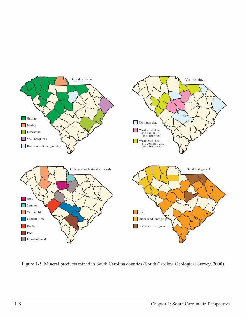
South Carolina produced $531 million in mineral commodities in 2001. This was nearly five times the value of minerals produced in 1980. Output from the Palmetto State’s 503 mines placed it 27th among the 50 states in nonfuel mineral production value and accounted for approximately 1.0 percent of the U.S. total. The leading product was cement (Portland and masonry), followed by crushed stone and construction sand and gravel. These three commodities composed about 90 percent of the State’s mineral production. Kaolin, industrial sand and gravel, and vermiculite were the next most important commodities by value. South Carolina ranked eleventh in the production of Portland cement, fourth in masonry cement, third in kaolin, eleventh in industrial sand and gravel, and first in vermiculite. Gold, which had been a significant commodity for more than 10 years, was not produced in 2001. Kennecott Mineral Co.’s Ridgeway Gold Mine ceased operations in the fall of 1999.

Active mines were reported in 44 of South Carolina’s 46 counties. Horry County led the State with 47 active mineral mines, followed by Aiken (34) and Charleston (33). Figure 1-5 shows South Carolina counties that produce stone products, clay, sand and gravel, and various minerals.

Cement production, which ranked first in value and third in tonnage, was worth $254 million for 3,310,000 metric tons. Portland cement made up $211 million of that production for 2,920,000 metric tons. Masonry cement constituted $43 million for 390,000 metric tons. Limestone is mined in Orangeburg and Berkeley Counties for the manufacture of cement and in Berkeley and Cherokee Counties as a source of agricultural lime.

Crushed-stone production was second to cement in value at $180 million and was first in tonnage with 27,200,000 metric tons. Rock types quarried and crushed for use as aggregate in concrete, macadam, and road construction include granite, limestone, and marl. Granite accounted for 79 percent of crushed-stone production and was valued at $147 million for 22,000,000 metric tons in 2000. Granite quarried for dimension stone from mines in Kershaw County was worth $855,000 for 9,230,000 metric tons in 1999. Dimension stone is extracted in blocks, mainly for use in buildings, monuments, and curbing. Limestone was second of the crushed-stone commodities, with a value of $24 million for 4,330,000 metric tons.

Construction sand-and-gravel placed third in value at $40 million and second in tonnage with 10,100,000 metric tons. With mines in 36 counties, sand-and-gravel production is the most widespread mining activity in South Carolina. It is mainly used as aggregate in concrete and asphalt and as fill. Industrial-quality sand is mined and processed in Lexington County for glassmaking, sandblasting, foundry, and filtration applications.

Kaolin ranked fourth in value at $20 million for 422,000 metric tons, or about $50 a ton. It is mined from numerous pits near the upper edge of the Coastal Plain and used in the paper, rubber, and ceramic industries.

Other important mineral commodities mined in South Carolina are vermiculite, manganiferous schist, sericite, and peat. Vermiculite’s principal use is as a soil-conditioning additive. It is also used as lightweight aggregate in concrete, plaster, and fireproofing. Manganiferous schist is mined for coloration in bricks. Sericite is processed for use as an inert filler in paint and expansion-joint cement, and peat is a soil conditioner.

Although not mined presently, gold has been an important resource since the early 1800’s. The mines yielded 300,000 troy ounces in three different eras: 1829–1858, 1866–1917, and 1931–1943. From 1985 to 1999, South Carolina produced about 1.7 million troy ounces from mines in Chesterfield, Fairfield, Lancaster, and McCormick Counties. South Carolina was the only gold producer east of the Mississippi River for much of that period, and the Ridgeway mine in Fairfield County was the largest producer (Table 1-2). Silver was a by-product of the gold mining. Other metals with production histories are copper, lead, silver, and tin.

Phosphate, used as fertilizer, was mined from 1867 to 1913 between Charleston and Beaufort. In 1938, reserves were estimated at 9 million tons. Encroaching development, environmental constraints, and production costs make it unlikely that this district will be mined again.


Figure 1-5. Mineral products mined in South Carolina counties (South Carolina Geological Survey, 2000).

Crushed stone

Sand and gravel

Sand

River sand (dredging)

Sand/sand and gravel

Granite

Marble

Limestone

Shell (coquina)

Dimension stone (granite)

Gold and industrial minerals

Kaolin

Cement (lime)

Sericite

Gold

Industrial sand

Vermiculite

Peat

Various clays

Weathered slate and common clay (used for brick)

Weathered slate and kaolin (used for brick)

Common clay


Table 1-2. Gold-mine production in South Carolina

Company Mine County year mining started

year gold production

ended

Total gold production

Kennecott Ridgeway Mining Company Ridgeway Mine Fairfield 1988 1999 1.4 million ounces.Figures from company.

Brewer Gold Company Brewer Mine Chesterfield 1987 1994 192,000 ounces. Figures from former employee.

Haile Mining Company Haile Mine Lancaster 19851 1992 86,000 ounces. Figures from company.

Gwalia Resources (USA), Ltd. Barite Hill Mine McCormick 1991 1995 - 1996 50,000–60,000 ounces.Estimated.

1Intermitent mining since 1829.

Sources: South Carolina Geological Survey and South Carolina Department of Health and Environmental Control

Today, 12.3 million acres, representing about 60 percent of the State’s land area, is forest land (Table 1-3). Timber is the largest cash crop, producing a delivered value of $876 million annually. Forest and wood products account for $5.4 billion worth of commodities and goods every year, or nearly 12 percent of the State’s economic output. The more than 30,000 people employed in forestry-related industry represent 9.3 percent of the State’s manufacturing employment and 2.5 percent of its total employment. Some aspect of forestry, whether it is growing, harvesting, or manufacturing, occurs in every county and benefits local, county, and regional economies. Figure 1-6 shows the distribution of the State’s primary forest-product manufacturing facilities.

Forestry

South Carolina has a rich forestry heritage, and timber production has been an important industry since the late 1600’s. The forest-products industry is the third largest manufacturing industry in the State, behind textiles and chemicals. Forests provide more than economic advantages, however. The State’s extensive forests provide habitat for wildlife, areas for outdoor activities, and enhancement of environmental quality. Forests contribute scenic beauty, improved water quality, erosion control, and recreational opportunities that range from hunting to bird watching. Monetary values are difficult to place on such benefits.

Table 1-3. Acreage of timberland by forest type and ownership in South Carolina – 2000

Forest type Public acres Private acres Total acres

Softwood types

White pine and hemlock 8,200 1,600 9,800

Longleaf and slash pine 182,800 364,000 546,800

Loblolly and shortleaf pine 557,400 4,855,100 5,412,500

Total softwood 748,400 5,220,700 5,969,100

Hardwood types

Mixed hardwood 75,300 1,351,700 1,427,000

Upland hardwood 204,400 2,188,600 2,393,000

Bottomland hardwood 207,700 2,262,300 2,470,000

Total hardwood 487,400 5,802,600 6,290,000

All types 1,235,800 11,023,300 12,259,100


Pulpwood is the leading timber product in the State. It accounted for 52 percent of total product output in 1999, while sawlogs, both hardwood and softwood, accounted for 38 percent. Ten percent of total product output came from miscellaneous products including peeler logs (mainly for plywood), poles, pilings, and posts.

About 23 percent of the timber harvested is hardwood and 77 percent is softwood. The primary species of managed timber is the loblolly pine. It grows on a wide range of soils and is indigenous to all but the extreme northwestern counties. Various oak species are the primary hardwoods harvested.

Individuals own about 74 percent of private-commercial forestland; the forest industry holds 16 percent. Ten percent of commercial forests are publicly owned, and the ownership is equally divided between national forests and other public lands.

Fish and Wildlife

A diversity of habitat in South Carolina supports a wide variety of animal life. More than 400 species and subspecies of birds can be found in the State. Endangered species that receive significant management priority include the Southern bald eagle, red-cockaded woodpecker, piping plover, and wood stork. South Carolina is one of the most important wintering areas for migratory waterfowl in eastern North America, and the wood duck is a year-round resident. The wild turkey and bobwhite quail are upland gamebirds that also are subjects of conservation efforts.

Mammals, likewise, are widespread and diverse. The large-game species and furbearers are managed statewide. Amphibians and reptiles are widespread, and several threatened and endangered species are present. These include the gopher tortoise, flatwoods salamander, gopher frog, American alligator, bog turtle, spotted turtle, and loggerhead sea turtle. The wide variety and abundance of freshwater and marine fishes supports an important commercial fish industry in the State and provides anglers with exciting recreation. Fish species are diverse and include trout from the coldwater streams in the Blue Ridge region, the famous land-locked striped bass of the Santee Cooper lakes, and marine game fish such as cobia, bluefish, and swordfish.

South Carolina can be divided into six major types of habitat: forested; grassland, cropland, and brush; coastal wetland; riverine wetland; aquatic; and beach (U.S. Army Corps of Engineers, 1972).

Forested. The forests of the State, exclusive of swamplands, can be separated into three types: deciduous, evergreen, and mixed. A major factor affecting the species located in these areas is the density of vegetative growth.

The deciduous forests support a diversity of species including wild turkey, mourning dove, numerous neotropical migratory songbirds, and raptors such as the

red-tailed hawk and great horned owl. Mammals common to this forest type include raccoon, opossum, gray squirrel, Southern flying squirrel, chipmunk, Eastern cottontail, whitetailed deer, and bear. The Eastern box turtle, black rat snake, Eastern hognose snake, copperhead snake, and various salamander species are representative of different amphibians and reptiles preferring the type of vegetation common to the hardwood forests.

Managed evergreen forests also support a wide array of wildlife. The longleaf pine ecosystem, although greatly reduced from historic levels, is among the most diverse of all forest systems, supporting hundreds of plant and animal species. The red-cockaded woodpecker, an endangered species, makes its home in pine forests where it prefers to live in old and diseased pine trees, particularly longleaf pine. Trees meeting these requirements are increasingly rare and are harder for the bird to find because of modern forest-management techniques.

The mixed forests have a wide variety of animal species common to both hardwood and evergreen forests. Many animal species have no difficulty adapting to different forest types as conditions and seasons change.

Grassland, Cropland, and Brush. These habitat areas consist mostly of agricultural lands but also include grasslands of improved and unimproved pasture and fields that have converted to brush. Parks and other vegetated zones of urban and suburban areas are included in this group.

Generally, only small birds and mammals are found near the fields and croplands, although larger mammals and birds of prey may feed and hunt here. Birds such as meadowlarks and sparrows are common, as is the cottontail rabbit, which is extremely widespread. Fallow fields and brushlands provide ideal management opportunities for quail and other grassland birds.

Coastal Wetlands. Both tidal and freshwater marshes make up this habitat. The freshwater marshes are the most important to waterfowl, although the salt marshes are used extensively by feeding ducks and geese. Rails, or marsh hens, are significant game birds, common in the salt marshes from Savannah to Murrells Inlet. Dabblers, diving ducks, and coot winter in the coastal area. Other occasional waterfowl include the Canada goose, blue goose, snow goose, and whistling swan. Coastal wetlands are also important as nesting areas for numerous bird species, including osprey and Southern bald eagle. Aquatic furbearers are found throughout the habitat and include muskrat, mink, and otter. The American alligator is found in the marshes and has reestablished itself owing to Federal protection.

Riverine Wetlands. This habitat consists mainly of wooded swamps along streams. Significant examples are the Santee Swamp, Four Hole Swamp, and Congaree Swamp. Flooding provides nourishment to the bottomland


hardwoods and cypress trees characteristic of the habitat and contributes an abundance and diversity of fauna and flora. Many bird species are found in riverine wetlands, including owls, hawks, and wild turkeys. Bachman’s warbler, a rare songbird, has been sighted in this habitat. Waterfowl, with the exception of the wood duck, do not nest in these areas. Small game and furbearing mammals are numerous and include rabbit, squirrel, opossum, raccoon, fox, muskrat, mink, and otter. Beaver colonies are found statewide, as are deer, bobcat, and black bear.

Aquatic. This habitat includes both marine and freshwater environments. The marine habitat is extensive along the entire coast and is found in the form of bays, sounds, inlets, and creeks. Approximately 160 species of saltwater fish are found in this area, of which most are inshore species. A few of the species are flounder, sheepshead, and striped bass. Offshore migratory species include tuna, mackerel, jacks, and bluefish, and examples of offshore bottom fish are black sea bass, snappers, and

porgies. Oysters, shrimp, and blue crabs are the most important commercial shellfish. Numerous shorebirds live in this area and include the American oystercatcher and the osprey.

Freshwater-fish habitats include the coldwater streams of the mountains, warmwater inland lakes, and blackwater streams of the Coastal Plain. Brook, rainbow, and brown trout are stocked annually where water temperatures are sufficiently cool. These streams are generally above 1,400 feet elevation. Warmwater fish, including bass, bream, catfish, and crappie, may be found in rivers, lakes, and ponds across the state. The Santee Cooper lakes (Marion and Moultrie) are the site of South Carolina’s famous striped bass (rockfish) fishery. These fish are managed intensively and are shipped to other lakes in the country. The lakes also are important waterfowl habitats.

Beach. Beach is the least extensive of all habitats in South Carolina. Beaches north of North Inlet are heavily developed and used for recreational purposes, and they

Figure 1-6. Locations of primary forest-product manufacturing facilities in South Carolina.

Chip mill

Fiberboard mill

OSB plant

Pulp and paper mill

Pole plant

Post mill

Saw mill

Veneer mill

EXPLANATION

40 miles10 0 10 20 30


consequently provide little wildlife habitat. The beaches south of North Inlet are less densely developed or are undeveloped, and they provide important habitat to the loggerhead turtle and brown pelican, two species that lay their eggs in the sand.

PHySIOGRAPHy AND GEOLOGy

The abundance, diversity, and beauty of the State’s water resources, including its mountain waterfalls, verdant swamps, Carolina bays, and valuable saltwater wetlands, are derived from a variety of physiographic domains. Those domains, broadly classified as the Blue Ridge, Piedmont, and Coastal Plain provinces, are the result of climatological and geological processes that occurred for many millions of years and that continue to alter the modern landscape.

Historical Overview

About 1.1 billion years ago North America’s ancestral continent, Laurentia, was deformed and metamorphosed by a collision of continents, and the mountain range formed by that event was worn down over the next several hundred million years. The Toxaway Gneiss of northwestern South Carolina is a remnant of those ancient events and is South Carolina’s oldest formation. Laurentia then began to rift (split and spread apart) 700 to 750 m.a. (million years ago), forming the Iapetus Ocean and a new eastern margin of North America. Evidence of the rift is found in the sedimentary and volcanic strata overlying the Toxaway Gneiss.

Several oceans formed off ancestral eastern North America during the Paleozoic Era in a series of continental rebounds and collisions that attached foreign terranes. Three collisional episodes occurred in the southern Appalachian Mountains, and a variety of sedimentary, volcanic, and metamorphic rock, plutons, folds, and faults in South Carolina’s Inner Piedmont reflect those episodes of 470 to 270 m.a.

Mesozoic rifting, about 200 m.a., broke up the Appalachians and led to formation of the Atlantic Ocean. During that period, one of the largest volcanic events in the earth’s history intruded diabase dikes and sills throughout the Piedmont and some Mesozic basins. Volcanism related to these dikes has been blamed for worldwide animal-life extinction at the end of the Triassic Period.

At the beginning of the Cretaceous Period (70 m.a.), uplift in the Blue Ridge and Piedmont produced an outpouring of deltaic and marine sediments that now compose about two thirds of the Coastal Plain stratigraphic section. During the Paleocene Period (68–58 m.a.), sea levels were lower and deposition on the Coastal Plain diminished. Miocene sea levels transgressed landward in several episodes (58–37 m.a.), and sand, silt, clay, and limestone were deposited over the middle and lower Coastal Plain. No major marine transgression

occurred again for nearly 30 million years, but a unique uplift in the Blue Ridge and upper Piedmont, 10 million years ago, produced an apron of stream-transported sediment across the upper Coastal Plain. Pliocene and Pleistocene marine transgressions in the past 2½ million years, caused by retreats and advances of continental glaciers, deposited thin but widespread marine sand and lesser carbonate layers across the Middle and Lower Coastal Plain. Figure 1-7 illustrates the structure of the rocks and aquifers formed during South Carolina’s geologic history.

Physiographic Provinces

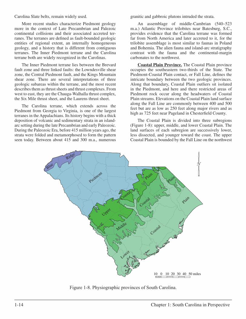
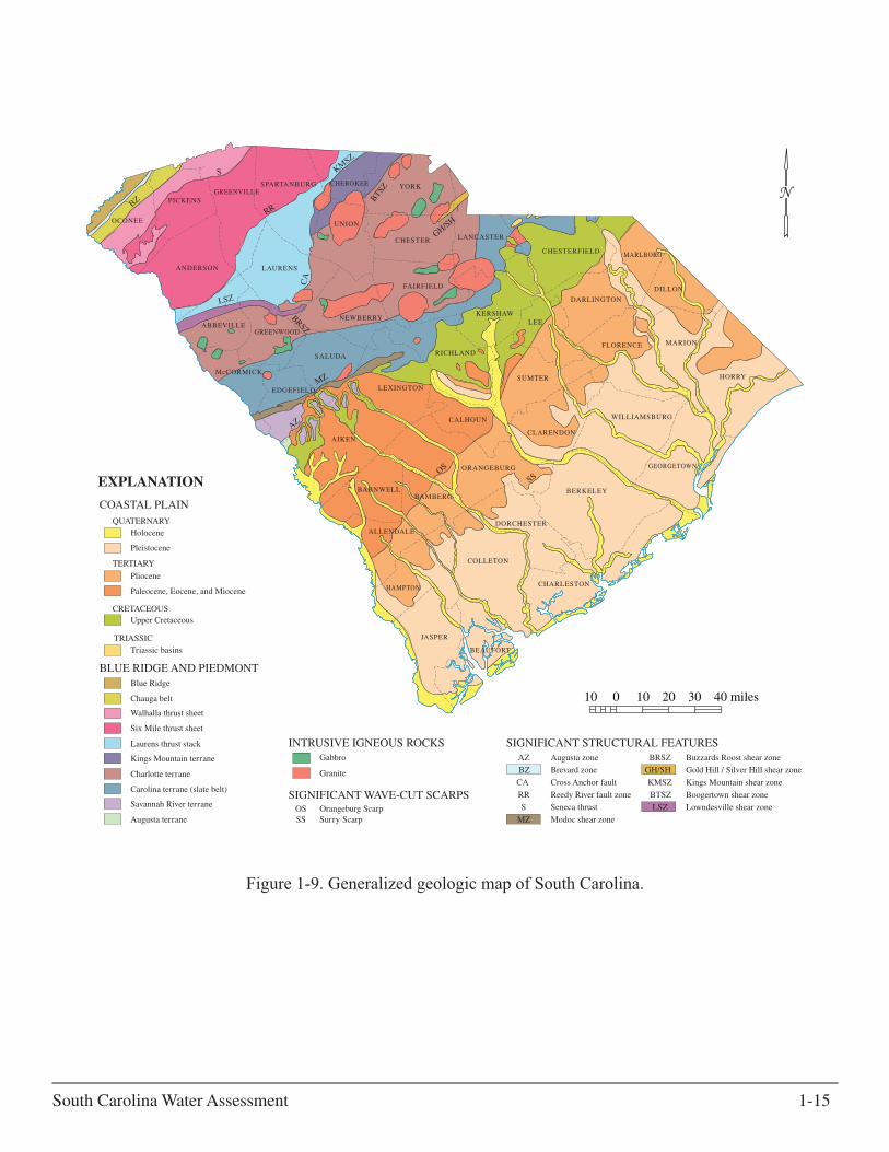
Blue Ridge Province. The Blue Ridge province occupies only 2 percent of the State’s land area and is located on the northwest edge of South Carolina (Figure 1-8). This mountainous region has elevations ranging from 1,000 feet in the foothills to 3,554 feet at Sassafras Mountain. Although physiographic and geologic boundaries usually coincide, northwestern South Carolina is an exception. The Blue Ridge-Piedmont physiographic boundary is the steep break in topography at the Blue Ridge front that trends N70ºE across northern Oconee, Pickens, and Greenville Counties. The Blue Ridge-Piedmont geologic boundary in this area is the N45ºE–trending Brevard fault zone. As the Blue Ridge front extends eastward from the Brevard zone across Piedmont geologic units, there is no correlation between the topography and the underlying rock formations (Figure 1-9).

The Toxaway Gneiss and the Tallulah Falls Formation represent the rocks of the Blue Ridge geologic province in South Carolina. The 1.2-billion-year-old Toxaway Gneiss has a restricted distribution just south of the North Carolina line. It typically is a medium-grained, prominently banded, quartzo-feldspathic gneiss. The Tallulah Falls Formation unconformably overlies the Toxaway Gneiss and is composed of schist and amphibolite. The gneiss, folded and metamorphosed during the Grenville orogeny, was folded and metamorphosed again with the Tallulah Falls Formation during the Taconic orogeny, and both formations were thrust northwestward during the Alleghanian orogeny.

Piedmont Province. The Piedmont province includes approximately 35 percent of the State and is between the Blue Ridge and Coastal Plain provinces. The topography is characterized by rolling hills that range in elevation from 1,000 feet near the mountains to about 400 feet at the Fall Line. A layer of chemically weathered bedrock called saprolite mantles the Piedmont in varying thickness.

Geologists recognized a pattern of northeast-trending lithologic belts in the Blue Ridge and Piedmont as early as the 1840’s. Later geologists classified these belts mainly by the varying degrees of rock metamorphism, and the names of these metamorphic regions, Blue Ridge, Brevard, Inner Piedmont, Kings Mountain, Charlotte, and


Figure 1-7. Generalized structure of geologic formations in South Carolina.

brbv

is

km

cgn

vu

vu

Mu Cvs

Km

Kbc

Tls

Tsd

Km

Kbc

Tls

Tsd

shallow

shallow

MSL

-1,000

-2,000

-3,000

-4,000

MSL

-1,000

-2,000

2,000

1,000

-3,000

-4,000

Feet

Feet

Kcf

Kcf

Triassicbasin

Kbc

TlsTsd

KmKcf

Shallow aquifer Floridan aquifer Tertiary sand aquifer Black Creek aquifer Middendorf aquifer Cape Fear aquifer

brbvis

cgnvuMuCvs

km

Blue Ridge beltBrevard beltInner Piedmont beltKings Mountain beltCharlotte beltCarolina Slate beltKiokee beltBelair belt

GEOLOGIC BELTS IN THE BLUE RIDGE AND PIEDMONT PROVINCES

AQUIFERS IN THE COASTAL PLAIN PROVINCE

Undifferentiatedcrystalline rocks

Undifferentiatedcrystalline rocks


Carolina Slate belts, remain widely used.

More recent studies characterize Piedmont geology more in the context of Late Precambrian and Palezoic continental collisions and their associated accreted ter-ranes. The terranes are defined as fault-bounded geologic entities of regional extent, an internally homogeneous geology, and a history that is different from contiguous terranes. The Inner Piedmont terrane and the Carolina terrane both are widely recognized in the Carolinas.

The Inner Piedmont terrane lies between the Brevard fault zone and three linked faults: the Lowndesville shear zone, the Central Piedmont fault, and the Kings Mountain shear zone. There are several interpretations of three geologic subareas within the terrane, and the most recent describes them as thrust sheets and thrust complexes. From west to east, they are the Chauga-Walhalla thrust complex, the Six Mile thrust sheet, and the Laurens thrust sheet.

The Carolina terrane, which extends across the Piedmont from Georgia to Virginia, is one of the largest terranes in the Appalachians. Its history begins with a thick deposition of volcanic and sedimentary strata in an island-arc setting during the late Precambrian and early Paleozoic. During the Paleozoic Era, before 415 million years ago, the strata were folded and metamorphosed to form the pattern seen today. Between about 415 and 300 m.a., numerous

granitic and gabbroic plutons intruded the strata.

An assemblage of middle-Cambrian (540–523 m.a.) Atlantic Province trilobites near Batesburg, S.C., provides evidence that the Carolina terrane was formed far from North America and later accreted to it, for the trilobite assemblage is most similar to faunas in Poland and Bohemia. The alien fauna and island-arc stratigraphy contrast with the fauna and the continental-margin carbonates to the northwest.

Coastal Plain Province. The Coastal Plain province occupies the southeastern two-thirds of the State. The Piedmont-Coastal Plain contact, or Fall Line, defines the intricate boundary between the two geologic provinces. Along that boundary, Coastal Plain outliers sit isolated in the Piedmont, and here and there restricted areas of Piedmont rock occur along the headwaters of Coastal Plain streams. Elevations on the Coastal Plain land surface along the Fall Line are commonly between 400 and 500 feet but are as low as 250 feet along major rivers and as high as 725 feet near Pageland in Chesterfield County.

The Coastal Plain is divided into three subregions (Figure 1-8): upper, middle, and lower Coastal Plain. The land surfaces of each subregion are successively lower, less dissected, and younger toward the coast. The upper Coastal Plain is bounded by the Fall Line on the northwest

Figure 1-8. Physiographic provinces of South Carolina.

Lower

Coasta

l

Plain

Piedmont

Blue

Ridge

Upper

Coastal

Plain

Middle

Coastal

Plain

50 miles10 0 10 20 30 40


PICKENS

OCONEE

GREENVILLESPARTANBURG

ANDERSON

ABBEVILLE

LAURENS

GREENWOOD

McCORMICK

EDGEFIELD

AIKEN

BARNWELL

ALLENDALE

HAMPTON

JASPER

BEAUFORT

CHARLESTON

GEORGETOWN

HORRY

DILLON

MARLBOROCHESTERFIELD

LANCASTER

YORKCHEROKEE

LEXINGTON

RICHLAND

CALHOUN

ORANGEBURG

BAMBERG

WILLIAMSBURG

BERKELEY

DORCHESTER

CLARENDON

SUMTER

KERSHAWLEE

DARLINGTON

FLORENCE MARION

CHESTER

FAIRFIELD

NEWBERRY

SALUDA

UNION

COLLETON

OS

SS

AZ

CA

RR

S

BRSZ

KMSZ

BTSZ

BZ

MZ

LSZ

GH/SH

SIGNIFICANT STRUCTURAL FEATURESAZ Augusta zone

BZ Brevard zone

CA Cross Anchor fault

RR Reedy River fault zone

MZ Modoc shear zone

S Seneca thrust

BRSZ Buzzards Roost shear zone

GH/SH Gold Hill / Silver Hill shear zone

KMSZ Kings Mountain shear zone

LSZ Lowndesville shear zone

BTSZ Boogertown shear zone

INTRUSIVE IGNEOUS ROCKSGabbro

Granite

OS Orangeburg ScarpSS Surry Scarp

SIGNIFICANT WAVE-CUT SCARPS

Augusta terrane

Blue Ridge

Charlotte terrane

Carolina terrane (slate belt)

Chauga belt

Laurens thrust stack

Six Mile thrust sheet

Walhalla thrust sheet

Kings Mountain terrane

Savannah River terrane

BLUE RIDGE AND PIEDMONT

COASTAL PLAINQUATERNARY

TERTIARY

CRETACEOUS

TRIASSIC

Holocene

Pleistocene

Pliocene

Paleocene, Eocene, and Miocene

Upper Cretaceous

Triassic basins

EXPLANATION

40 miles10 0 10 20 30

Figure 1-9. Generalized geologic map of South Carolina.


and the Orangeburg Scarp on the southeast. The terrain is characterized by an erosional topography of relatively high relief and high drainage density similar to the lower Piedmont, and it contrasts with the constructional topography to the east. The gently undulating upland surfaces and the underlying soils of the upper Coastal Plain are old: the thick, mineralogically mature soils may be 10 million years old, or an order of magnitude older than the thinner and less mature soils of the Piedmont. Quartz sand derived from the fluvial erosion of the upper Cretaceous and lower Tertiary units during the late Miocene to early Pliocene was transported northeastward by wind to form the largest dune field in the southeastern U.S. Many dunes preserve a distinctive dunal topography and are up to a mile across and 100 feet thick. The contrast in topography between the upper Coastal Plain and the more subdued land surfaces of the middle and lower Coastal Plains suggests that most upper Coastal Plain uplift and erosion occurred prior to deposition of the Pliocene and Pleistocene marine units of the middle and lower Coastal Plain.

The middle and lower areas of the Coastal Plain are distinguished by a stair-stepped topography of terraces separated by scarps. Each successive terrace is younger and lower toward the coast. The advances and retreats of massive continental glaciers caused a series of sea-

level highstands during the Pliocene and Pleistocene that deposited the terraced formations. The middle Coastal Plain lies between the Orangeburg Scarp and the Surry Scarp. It is underlain by two upper Pliocene formations separated by the Mechanicsville-Parler Scarp. The region is a gently rolling to flat terrain dissected by transverse streams and locally covered by Quaternary eolian, lacustrian, and alluvial deposits. Elevations range from 215 to 100 feet. The lower Coastal Plain is between the Surry Scarp and the present shoreline. Pleistocene and Holocene deposits underlie the surface.

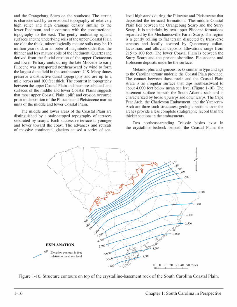
Metamorphic and igneous rocks similar in type and age to the Carolina terrane underlie the Coastal Plain province. The contact between those rocks and the Coastal Plain strata is an irregular surface that dips southeastward to about 4,000 feet below mean sea level (Figure 1-10). The basement surface beneath the South Atlantic seaboard is characterized by broad upwarps and downwarps. The Cape Fear Arch, the Charleston Embayment, and the Yamacraw Arch are three such structures; geologic sections over the arches provide a less complete stratigraphic record than the thicker sections in the embayments.

Two northeast-trending Triassic basins exist in the crystalline bedrock beneath the Coastal Plain: the

Figure 1-10. Structure contours on top of the crystalline-basement rock of the South Carolina Coastal Plain.

-500

EXPLANATION

Elevation contour, in feet relative to mean sea level

0

-100

-300

-500

-1,00

0

-1,500

-2,000

-2,500

-3,000

-3,500

-4,000

0-100

-200

-300

-400

-500

-1,000

-1,500

-2,000

-2,500

-3,000

-3,500

-4,000

FALL

LINE

50 miles10 0 10 20 30 40


Dunbarton Basin that underlies the Savannah River Site in Barnwell County and the Florence Basin below the Florence area. The large, east-west trending South Georgia Basin extends from South Carolina to Mississippi. It underlies the South Carolina Coastal Plain south of a line between Allendale and Georgetown, and basin sediment consists of red siltstone, sandstone, and some limestone pebbles.

Geologic Formations

Upper Cretaceous Formations. The Middendorf Formation is composed of light-colored, crossbedded, kaolinitic sand with lenses of white, tan, red, and purple kaolinitic clay exposed at the surface southeast of the Fall Line. The thickness ranges from a few feet at the Fall Line to 1,060 feet in Beaufort County. The top of the unit dips from a depth of about 50 feet below the land surface in the northern part of the Coastal Plain to about 2,800 feet in Beaufort County.

The Black Creek Formation is composed of dark-gray to black laminated clay with white or gray phosphatic, lignitic, and glauconitic sand, and light-gray sand interbedded with dark-gray marine clay. The formation is exposed along Black Creek a few miles above Darlington. The Black Creek Formation near Sumter is 285 feet thick and occurs from 50 feet above sea level to 235 feet below sea level. At Charleston the top of the unit is 815 feet below sea level, and the base is at about 1,800 feet. At Beaufort, the Black Creek is 2,100 to 2,800 feet below sea level.

The Peedee Formation crops out between Florence and Georgetown Counties. It consists of dark-gray clay interbedded with fine to medium micaceous and glauconitic sand and streaks of hard shelly limestone and siltstone. Dark marine-clay interlayers up to 6 feet in thickness occur but are subordinate. Burrows are common, and the bioturbation may account for the massive character of Peedee sand beds. The top of the formation ranges from 70 feet below mean sea level in the Orangeburg area to more than 1,700 feet in Beaufort County. Thickness of the formation varies from a few feet near the updip limit to 360 feet in the Beaufort area.

Paleocene Formations. Today the Black Mingo is recognized as a group that includes the lower Paleocene Rhems Formation and upper Paleocene Williamsburg Formation in the lower Coastal Plain and the upper Paleocene Lang Syne Formation in the upper Coastal Plain. The Rhems Formation is a light-gray to black shale interlaminated with thin seams of fine-grained sand and mica. The Williamsburg Formation consists of fine-grained silicified mudstone; fossiliferous, laminated, sandy shale; glauconitic, clayey, fossiferous sand; and indurated, molluscan-rich limestone. The Lang Syne Formation is composed of glauconitic, pebbly, poorly sorted sand; thin-bedded, micaceous, medium-grained quartz sand interlayered with clay laminae; and thick dove-gray to

black beds of fullers earth. The Lang Syne Formation overlies upper Cretaceous strata in exposures in Lexington, Richland, Calhoun, Sumter, and Lee Counties.

Lower and middle Eocene Formations. The updip Fourmile Branch Formation and downdip Fishburne Formation are subsurface units apparently of the same lower Eocene depositional sequence. The Fourmile Branch Formation consists of as much as 30 feet of mainly orange, green, yellow, or tan, moderately to well-sorted, fine- to coarse-grained quartz sand. Green and gray clay beds, several feet thick, occur in the middle and upper parts of the unit. The Fishburne Formation, named for Fishburne Creek in southern Dorchester County, is a greenish-gray, glauconitic, impure, clayey, fine-grained, poorly stratified limestone. Thin (24 to 74 feet thick) but laterally persistent, the unit occurs near the coast and southwest of the Charleston-Summerville area.

The Huber and Congaree Formations, exposed in the upper Coastal Plain, are updip-downdip facies variants of a Lower Eocene to lower middle Eocene sequence. The Huber Formation is characterized by distinctive, cross-bedded, poorly sorted, generally coarse sand with kaolin balls, and commercial kaolin deposits are found in the upper part of the unit. Its lower part consists of thinly layered, well-sorted, fine-grained sand with minimal interstitial clay and thin, laterally continuous clay interlayers. The Huber Formation grades downdip into medium-grained, cross-bedded quartz sand of the upper part of the Congaree Formation and green, thinly layered, indurated claystone in the lower part of the unit. The Huber and Congaree Formations are about 60 feet thick throughout their outcrop area. In the Tertiary outcrop area above the Orangeburg Scarp, the Huber-Congaree depositional sequence is, by far, the most widespread stratigraphic unit. From Aiken County along the Fall Line to Lexington County, a distance of 39 miles, the Huber Formation overlaps upper Cretaceous strata and lies directly on Piedmont crystalline rocks. The Congaree Formation caps the hilltops throughout the High Hills of Santee in western Sumter and Lee Counties.

The Warley Hill Formation is a distinctive lower Middle Eocene unit composed of dark-green, glauconitic, quartz sand. It has an outcrop area confined to southern Calhoun and northern Orangeburg Counties and is generally 5 to 20 feet thick. The unit grades downdip into glauconitic, calcareous beds in the lower Coastal Plain. In Orangeburg County, the strata include the oyster Cubitostrea lisbonensis, a guide fossil to the lower middle Eocene.

Like the Huber-Congaree, the McBean Formation and Santee Limestone are updip-downdip facies of the same middle Eocene depositional sequence. The McBean Formation overlies the Warley Hill Formation and in South Carolina is composed of pale-green, fine-grained, cohesive clayey sand. In Georgia, the unit is a cream-white marl at its type locality. The McBean Formation is restricted in the


upper Coastal Plain to the region between the Savannah and Congaree Rivers, and it is characterized by two middle Eocene guide fossils, the oyster Cubitostrea sellaeformis and the clam Pteropsella lapidosa.

The Santee Limestone is a creamy yellow to white, fossiliferous, indurated sediment that crops out in a belt, about 25 miles wide, from Allendale County on the Savannah River eastward to the Santee River. In the northern part of its outcrop area, the formation contains numerous caverns and sinkholes related to karst topography.

The Orangeburg District bed and Castle Hayne Limestone are updip-downdip facies of the uppermost middle Eocene depositional sequence. The Orangeburg District bed overlies the McBean Formation and is composed of well-sorted, fine- to medium-grained to poorly sorted, medium- to very-coarse-grained sand with minor interstitial clay. The formation is commonly pale yellow with black manganese oxide splotches and with very thin interstratified green clay laminae. Pale green beds of quartz sand with some glauconite occur in the lower part of the unit. Like the McBean Formation, the Orangeburg District bed is restricted in the upper Coastal Plain to south of the Congaree River. A fossil assemblage in the unit at Orangeburg contains 91 molluscs, including the clam Glyptoactis (Claibornicardia) alticostata, a guide fossil to the uppermost middle Eocene Gosport Sand of the Gulf Coast region. The Castle Hayne Limestone of the middle and lower Coastal Plain is composed of buff to gray, crumbly fossiliferous limestone. The Crassatella alta-bearing limestone beds of the middle and lower Coastal Plains are the downdip carbonate equivalent of the Orangeburg District bed and have been called the Cross Formation.

Upper Eocene and Oligocene Formations. The Dry Branch Formation and the Tobacco Road Sand of the upper Coastal Plain are the lower and upper stratigraphic units of the upper Eocene. The two formations are distinctive and readily mappable. They represent the transgressive and regressive facies of a single depositional sequence. Exposures in Aiken County show wispy clay laminae extending from the uppermost Dry Branch Formation into the very-coarse-grained sand-and-pebble bed at the base of the Tobacco Road Sand, demonstrating continual sedimentation at the contact. The units occur between the Congaree and Savannah Rivers. The Dry Branch Formation typically is composed of poorly-sorted, cross-bedded, golden-yellow sand with beds of green montmorillonite clay in the lower part of the unit and interstratified thin clay layers in the upper part. It is commonly 30 to 40 feet thick. The formation lies on the Orangeburg District bed and overlaps that unit to lie directly on the Congaree Formation. The Tobacco Road Sand is composed of red, purple, or lavender poorly-sorted sand beds, commonly with abundant white, clay-lined burrows. The base of the unit is marked by a 1- to 3-foot clayey, discoidal

quartz-pebble bed. The stratum is a distinctive marker bed throughout Aiken and Barnwell Counties and ranges from 30 to 60 feet in thickness. The two formations extend updip to the edge of the Coastal Plain except in parts of Edgefield and Lexington Counties. The Dry Branch Formation and Tobacco Road Sand grade downdip into the Ocala Limestone, the Harleyville Formation, and the Parkers Ferry Formation.

Three formations are generally within the grayish-green marl of the Cooper Group (formerly Cooper Marl or Formation): the late Eocene Harleyville and Parkers Ferry Formations and the Oligocene Ashley Formation. The Harleyville is a compact, phosphatic, calcareous clay, and the Parkers Ferry is composed of glauconitic, clayey, fine-grained limestone with abundant microfossils and locally abundant mollusc and bryozoan fragments. The Ashley Formation is made up of phosphatic, muddy, calcareous, fine-grained sand. The upper Oligocene Chandler Bridge Formation and the uppermost Eocene to lowermost Oligocene Drayton limestone beds now are included, respectively, at the top and middle of the group by recent researchers. The Chandler Bridge Formation is a fossiliferous, noncalcareous phosphatic sand with diverse whale fauna.

Miocene Formations. Near Charleston, three lower Miocene units and one upper Miocene unit have been recognized. The three lower Miocene units include the Tiger Leap Formation, the Parachucla Shale, and the Marks Head Formation. The Tiger Leap Formation is a phosphatic, shelly calcarenite with a patchy distribution. The Parachucla Shale is an olive-gray, dense, silty clay that occurs in the western part of the Charleston area. The Marks Head Formation is an olive-brown, clayey, quartz phosphate sand that is the most widespread of the Miocene units. The upper Miocene Ebenezer Formation is composed of shelly shelf sand and occurs in two small patches between Moncks Corner and Harleyville.

Northwest of the Orangeburg Scarp, a fluvial upland unit of late middle Miocene to early late Miocene age occurs on the high parts of the interfluves. The formation is composed of poorly-sorted, very-coarse-grained, clayey sand or clayey grit that locally includes abundant, well-rounded quartz cobbles 3 to 4 inches in diameter. Remnants of the formation extend from western Lee County southwestward into Georgia. From Lee County, where the upland unit overlies the lower to lower-middle Eocene Congaree Formation, the unit overlies younger marine formations toward the southwest. The widespread distribution of the fluvial sediments in the upland unit reflects uplift of the southeastern Blue Ridge approximately 10 million years ago.

Pliocene Formations. The middle and lower parts of the Coastal Plain are distinguished by a stair-stepped topography of marine terraces bounded by scarps. Each successive terrace is younger and lower as the present


shoreline is approached. The middle Coastal Plain, a gently rolling to flat terrain with transverse streams, is underlain by Pliocene marine sediment locally covered by Quaternary eolian, lacustrian, and alluvial deposits. Elevations range from about 215 to 100 feet. The middle Coastal Plain surface is underlain by the upper Pliocene Duplin Formation, exposed in a belt just southeast of the Orangeburg Scarp, and the uppermost Pliocene Bear Bluff Formation, separated from the Duplin by the Mechanicsville-Parler Scarp. The fossiliferous marine-shelf sand beds of the Duplin Formation record the maximum Plio-Pleistocene marine high stand, an inundation that reached Orangeburg and that formed the prominent Orangeburg Scarp.

In the Charleston area, the Pliocene is covered by Pleistocene units and encompasses the lower Pliocene Goose Creek Limestone and the upper Pliocene Raysor and Duplin Formations. The Goose Creek Limestone is a

quartzose calcarenite widespread near the Cooper River but patchy elsewhere. The Raysor Formation crops out on the Edisto River and consists of shells in a blue-mud matrix; it is absent at Charleston and may have been stripped by erosion. The Duplin Formation occurrence is patchy.

Pleistocene Formations. Pleistocene stratigraphic units underlie the lower Coastal Plain, separated from the middle Coastal Plain by the Surry Scarp. The units are thin, marine formations that are dominantly composed of quartz sand. Seven Pleistocene formations have been recognized, each one underlying a separate terrace. From oldest to youngest they are the Lower Pleistocene Waccamaw and Penholoway Formations, the middle Pleistocene Canepatch Formation and Ten Mile beds, and the upper Pleistocene Socastee Formation, Wando Formation, and Silver Bluff beds.

chapter 1 - south carolina department of natural resources

Documents