Chapter 1 - Secondary Ports ?? If you can work with secondary ports try the exercise on page 13.

Applicable references for this section are YN on Secondary Ports and NH chapter 7.

The Tiller CD interactive modules on Secondary Ports will help you with this lecture.

All our tidal work so far has been with ports that have their own tide tables and tidal curves. Generally speaking, these are large commercial ports where the expense of producing and maintaining this data can be justified.

Many small harbours are attractive to us as yachtsmen and women. They may be more picturesque or just more pleasant than the bigger ports with their constant flow of large shipping. We need tidal information for these places but it is not practical to provide it on a harbour by harbour basis. Actually, we probably don't really want it! The volume of information would be huge and would take up too much space on many yachts.

We need (and we have) a way to relate the small harbours to the main commercial ports and this is the subject of this chapter.

There are two more definitions that we need:

1. A STANDARD port is one for which there are tide tables and a tidal curve. 2. A SECONDARY port is one for which information is available that RELATES it to a

standard port.

As Day Skippers you will be aware that secondary ports exist but will probably not have studied them in depth.

The sort of harbour we are concerned with is frequently a secondary port. We will consider two ways to find out the tidal information for this type of port and, in ascending order of accuracy, usefulness and the amount of work required, they are:

• The tide level data on a chart. • The secondary port tidal data from the almanacs (there are excerpts in the TA - N).

First, though, let's investigate the principles a little deeper.

What is a secondary port? The RYA course is built around an artificial world with realistic tidal data and information. This means that whilst we will be working with a good example of the tidal environment it does not relate to any identifiable area of the real world.

You might reasonably ask whether this is a good idea so, to prove the point, let’s start with a brief look at a real world example.

Tidal flows

The English Channel (Figure 1) is a typical, if complex, example of coastal waters. The flood tide sweeps East up the Channel and meets the South flowing North Sea tides. Add the uneven coastlines and the flows in and out of the River Thames and it is small wonder that matters are complex in this area.

There are two points of interest as far as we are concerned:

1. As the flood tide flows east it is squeezed as the English Channel gradually narrows. We know that if we dam a stream the water level behind the dam rises and there is a somewhat similar effect in the Channel. We would expect, therefore, to find that tidal heights vary from harbour to harbour. The combination of different physical characteristics in each harbour and the 'dam' effect of the Dover straits make this inevitable.

2. High tide is a moving event in the English Channel. It takes about six hours to run from Falmouth to the Dover Straits. We would therefore expect to find timing differences between ports as we move along both coasts of the English Channel.

Characteristics of a secondary port ?? Can you remember the definition of a secondary port?i

We’ll use Dawson Harbour on page 86 of the TA - N as an example.

?? Find it in the TA - N and familiarise yourself with the layout used in the TA - N. Is it consistent for all ports? Remember that a secondary port:

1. Is near to a standard port and we are told which port that is (Colville). 2. Shares the same tidal curve as the standard port. In other words the tidal characteristics

are pretty similar and this is a good enough approximation. 3. Has its own tidal heights and/or times. They differ from the standard port and we are

given information on this in tabular form in the block just below the words 'Standard Port Colville’.

In the case of Dawson Harbour, there is then a mass of information about the port itself, including a handy chartlet.

Tidal level data Here is a quick and easy way to get general tidal height information when planning a passage or for rough and ready pilotage. Some charts contain tidal level data.

?? Both practice charts have this information so make sure you can find it now. Keep RYA3 open when you have found it.

We can see that there are data for a number of ports on the chart. For each port we have a position and mean HW and LW levels for springs and neaps.

Colville (page 78) is a STANDARD port - we know this because it has its own tide table and tidal curve. Dawson is a secondary port tied to Colville and has no tide tables but its own curve. The TAN talks of a tidal anomaly at Dawson. This means that its HW time cannot be sensibly predicted though the height can. Everything therefore works around LW time for a port like Dawson. On RYA3 there is no tide level data given for Dawson Harbour but there is an entry for St. Kilda a few miles to the north. We will use this to get a general understanding of the area.

English Channel tidesEnglish Channel tides

River Thames

North Seatidal stream

English Channel

SolentCalais

Flood tide moves East

Dover HW - 3Dover HW - 3

FranceCherbourg

Dover Straits

Falmouth

Figure 1 - Dover HW -3

So, how can we use this information? Some examples will make the point.

1. At MLWN how much water is over the drying rock (45 47’.2N 05 59’.1W) just S of Montague Island?

Answer - MLWN at St. Kilda is shown as 2.3m. The rock has a drying height of 0.3m so will be covered by 2.0m at MLWN.

?? Will it be visible at MLWS?ii

2. ?? On chart RYA4A could a yacht drawing 2.0m pass between Old Dawson and Inner Rocque at MLWS and MLWN?iii

This is a quick and easy way to understand tidal heights and a useful way of handling questions like the ones above. We can use it to decide whether a bank can be crossed, or a bridge cleared, but it is only accurate at mean neaps or springs. We need a general technique to handle secondary ports.

Secondary port calculations ?? Just a reminder – can you define a secondary port?iv

You might reasonably observe that what follows is quite a lot of work. ‘Surely we can guess it accurately enough?’ is a common observation. These days we might also note that tidal heights can be readily predicted by computer. You are, of course, right and for many situations a reasonably accurate ‘educated guess’ is good enough.

Computers give us facts but they do not help us to understand questions such as ‘if we are 20 minutes late can we still cross the shallows between Old Dawson and Inner Rocque in an offshore gale with high pressure affecting the height of tide at HW +6?

The techniques in this chapter will improve your understanding of secondary ports and therefore your ability to make valid approximations and reliable calculations.

Approach

Before we go delving into the tide tables let's stop and think for a moment. If we are going to use the tide tables and curves to get the answers for a secondary port there are going to be some differences in technique. Here is what we do:

1. Convert the problem to a solvable form - no change in the procedures we learnt earlier. 2. Find the tidal cycle we want to use and extract the STANDARD port times and

heights of tide - no change in procedure. 3. Convert the tide times and heights for the standard port so that they are correct for

the SECONDARY port - this is the only extra step. In effect we are going to create the secondary port’s tide table for the tidal cycle (flood or ebb) encompassing the time and date we are interested in.

4. Use the SECONDARY port information with the curve for the STANDARD port. There is no change to the way that we use the curve - all we are doing is to replace the standard port data (step 2 above) with the secondary port's data.

It is really very straightforward so let’s take it step by step and then pull it all together with a worked example.

Secondary port information

?? Open the TA - N at page 86 and find the entry for Dawson Harbour. From the top it covers:

1. The charts that cover the port - this is useful particularly when planning a passage.

2. The standard port to use – it is Colville. The arrow tells us which way in the TA - N (or almanac) to go to find the standard port's data.

3. The tidal differences block - this is the key to secondary port calculations. 4. ‘Differences Dawson Harbour' - with more times and heights.

The tidal differences block

This is the heart of the secondary port process. It contains time information (Figure 2) and height information (Figure 3).

Time difference

The section on timing (Figure 2) has two parts:

The upper section relates to the standard port and gives typical HW and LW times at that port.

The lower section relates to the secondary port. For Dawson it is simple. It tells us that HW Dawson is somewhere between 38 and 14 minutes earlier than at Colville. It also tells us that LW is between 6 and 30 minutes earlier than at Colville.

?? Contrast this with Sandquay (TA - N page 84) where the differences are much smaller and where, in practice, we might well ignore them. The reason for this is, of course, that Sandquay is much closer to Colville and so we might expect the differences to be much smaller.

We now have the information to allow us to work out (by interpolation) an accurate time DIFFERENCE for any particular tide.

Before we investigate interpolation let's look at the other half of the tidal differences block and see what it tells us about height differences. The interpolation techniques we use are similar, so we can study both at the same time.

Height differences

The upper figures (Figure 3) are the mean heights for the primary port. The lower ones are the height difference for the secondary port for each of the four mean heights.

Our requirement is similar to that for time. Given the differences for mean HW and LW at neaps and springs we need to be able to work out the secondary port's height differences for any tide.

Using the data

Let's take the simple case first. At mean spring tides and mean neap tides we can very often simply apply the corrections that are given. You probably did this on your Day Skipper course but here is an example for you

Secondary port times Secondary port times

TimesHW LW 0100 0700 0100 0700 1300 1900 1300 1900 Differences Dawson Harbour BRAYE-0038 -0014 -0030 -0006

These are ‘typical’HW and LW times forthe STANDARD port

These are the TIME differences for the secondary port

Figure 2 - Secondary port times

Secondary port heights Secondary port heights

MHWS MHWN MLWN MLWS 4.8 3.9 1.4 0.5

+2.8 -+1.7 +1.0 +0.5

These are the STANDARD port mean tidal heights

These are the height DIFFERENCES for the SECONDARY port

The height of MHWS at Dawson is 7.6m (4.8+2.8)

Figure 3 - Secondary port heights

to work through.

?? Work out the height and time of HW (around midday) and the following LW at Dawson on September 7th.v

This is reasonably straightforward but we do need a generalised technique to handle any tide time and height correctly.

The sequence is important

Always convert to DST AFTER applying the secondary port correction.

?? Can you work out why?vi

Working with any tidal range Making an 'educated guess'

If the tidal range is between springs and neaps we can often make a very good assessment by inspecting the secondary ports’ information. At Sandquay (TA - N page 84) the time difference is going to be between six and ten minutes for HW and it is always six minutes for low tide.

The heights are similar; at LW we always subtract 0.2m. At HW we are edging towards the need to interpolate correctly. At mean springs we need to add 0.4m and at mean neaps subtract 0.1m. We will often be able to get away with an educated guess and be accurate enough but the error in the height of tide could certainly be around 0.25m if we get it wrong.

With small differences such as these nobody, in reality, is going to argue over an interpolation approach that says it is mean springs, mean neaps or midway. For Sandquay, the error from this approach will be very small on the time of high or low water. With the height of tide we could however introduce a small but appreciable error at high tide that might be significant.

In practice, this is often good enough. We are making a very simple interpolation and effectively we can say that the 'difference' to be applied is one of three values - the neap difference, the spring difference or half way between.

If we can allow a safety margin then this gives a reasonably accurate and useable answer. The error will not be more than half of the variation between the neap and spring difference.

Using a pro forma for secondary tide approximations

There are times, and Dawson is a good example, when we may need a more accurate technique. There will also be occasions when our boat is bouncing up and down and we are tired or sea sick. Dawson is actually an example of a port where the tidal curve is

given for it, although it is a secondary port. More of this later.

A systematic approach helps eliminate errors and speeds up our calculations.

?? Note that YN and NH use a slightly different approach. We think that ours is easier but, if you get the right answers, any technique is correct.

In this course we teach you how to use a simple pro-forma to work out the secondary port times and heights in a graphical manner. There are many variations and, if you have a preferred technique, please use it. We will soon tell you if it does not give the right answers!

Our approach is built around a form (Figure 4) and there is a full size copy on page 7.

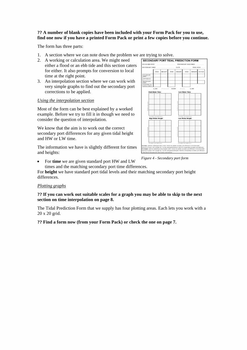
?? A number of blank copies have been included with your Form Pack for you to use, find one now if you have a printed Form Pack or print a few copies before you continue.

The form has three parts:

1. A section where we can note down the problem we are trying to solve. 2. A working or calculation area. We might need

either a flood or an ebb tide and this section caters for either. It also prompts for conversion to local time at the right point.

3. An interpolation section where we can work with very simple graphs to find out the secondary port corrections to be applied.

Using the interpolation section

Most of the form can be best explained by a worked example. Before we try to fill it in though we need to consider the question of interpolation.

We know that the aim is to work out the correct secondary port differences for any given tidal height and HW or LW time.

The information we have is slightly different for times and heights:

• For time we are given standard port HW and LW times and the matching secondary port time differences.

For height we have standard port tidal levels and their matching secondary port height differences.

Plotting graphs

?? If you can work out suitable scales for a graph you may be able to skip to the next section on time interpolation on page 8.

The Tidal Prediction Form that we supply has four plotting areas. Each lets you work with a 20 x 20 grid.

?? Find a form now (from your Form Pack) or check the one on page 7.

Figure 4 - Secondary port form

Figure 5 - Secondary port form

The scale that you use should not affect the answer.

Too small a scale will, however, make your life harder!

Let’s take a couple of examples

1. If, for example, you were working with a six hour time span (e.g. 07:00 to 13:00 with Dawson Harbour (TA – N page 86) you could use one, two or three squares per hour for the standard port times. The last one is the best choice because it uses the graph to its full extent (18 of the 20 squares are used) and this means that one square represents 20 minutes as opposed to 30 or 60 minutes. For the HW secondary port differences you could use a 30 minute scale (running from – 10 minutes to – 40 minutes) with one square on the graph representing two minutes.

2. Similarly with heights. For Dawson Harbour HW heights we could use a standard port scale running from 3 to 5 with one square on the graph representing 0.1m. For the differences a scale running from +1 to +3 does the job nicely and, again, each square represents 0.1m.

?? Use the biggest scale that you can. If you are working with a seven hour time span what scale would you use?vii

Handling time

We will almost always need to work out the HW time of the secondary port and, depending on the problem we are solving, we may need the time of LW as well. The same technique is used for both.

The assumption is that the secondary port differences are directly PROPORTIONAL to the standard port's information.

?? We want to know the time of HW at Dawson on May 10th. The time of HW at Colville is 11:07 zone time. At this stage we must work with UT because the HW times used to work out the correct difference are ALWAYS given in zone time (zone – 0100 or zone –1 for Dawson and Colville).

By inspection of the four HW numbers given for Dawson (the upper block in Figure 2) we can see that 11:07 falls between 07:00 and 13:00.

?? Take a secondary port form and work with it now.

1. Decide on the scales to be used and mark up the graph (figure 6). 2. Match the pairs of points (standard port time and its matching secondary port difference)

and mark them on the graph. In this example 07:00 matches - 00:14 to make one point on the graph. The other pair, obviously is 13:00 and - 00:38. Matching them correctly is critical.

3. Draw a line linking the points. Figure 6 shows you the completed graph. 4. Mark in the time (11:07) on the appropriate axis and read off the difference from the

other. The answer in this case is – 30 minutes. The graph may let us work to a better accuracy than this but, in reality, it is meaningless. The nearest minute is good enough.

Figure 6 - Time

You must draw the graph so that the differences and times are paired correctly. This is vitally important and a common cause of error.

Interpolating heights

The process is very similar. The height of HW at Colville in our example is 4.3 m.

The three steps (Figure 7) are:

1. Work out suitable scales. 2. Mark in the correct points on the graph

block and draw a line joining them. 3. Work out the applicable difference for a

HW height of 4.3m. The difference is +2.2m.

?? You’ve got a choice now - either follow through the worked example that follows or have a go with the questions on page 12.

Worked Example ?? Find a blank tidal prediction form from your Form Pack and let’s get going.

We will stick with Dawson Harbour because the differences are big enough that an ‘intelligent’ guess is unlikely to be good enough. The problem we are going to solve is this:

‘At what time can I cross the drying rock 0.3m just south of Montague Island to the north of Dawson Harbour (see TA – N page 87) with 1.0m clearance and a draught of 2.5m during the morning of September 18th on the flood tide? We will work out the heights and times of HW and LW and then use the right tidal curve to solve the problem.

The process is outlined below and the answers are on page 10. We suggest that you either try your hand at each step and then check with our answer or take a peek at the worked Tidal Prediction Form (Figure 8 on page 11) before you begin.

Important note: The Tidal Prediction Form and curve use some colour to aid clarity. In reality of course there’s no need to use anything but a pencil.

Step 1 - convert the problem to a solvable form. In other words restate the problem in a way that we can handle with the tide tables and curves

Step 2 - Find the standard port data and enter it on the Tidal Prediction Form

Step 3 - Create what is in effect the tide table for the secondary port for the date and tidal cycle(s) of interest. We do this by marking up the graphs with the secondary port data and then using the differences to modify the standard port times and heights. Either have a go first or take a quick look at the worked example before you make up your own.

Step 4 - now answer the questions.

Figure 7 - Height

Answers to worked example You will find the completed secondary port form in Figure 8 and the tidal curve in Figure 10.

Step 1 - convert the problem to a solvable form. In other words restate the problem in a way that we can handle with the tide tables and curves

Answer - we need to find the time during the morning flood on September 24th at which the height of tide will be 3.8m. (The required depth is 3.5m and we have a charted drying height of 0.3m so the required height of tide will be 3.8m).

Step 2 - Find the standard port data and enter it on the Tidal Prediction Form

Answer - see the Tidal Prediction Form - yours should be the same and note that we are using zone time not summer time at this stage. The secondary port differences are based on zone time so it would be wrong to convert HW and LW times to summer time now - we do it later.

Step 3 - Create what is in effect the tide table for the secondary port for the date and tidal cycle(s) of interest. We do this by marking up the graphs with the secondary port data and then using the differences to modify the standard port times and heights. Either have a go first or take a quick look at the worked example before you make up your own.

Answer - Mark up each of the graphs with the standard port data (see TA - N page 40) and Dawson differences. The worked example shows you how the end result should look. Don’t worry if your graphs use different units. There’s no harm in this but as a general rule we tend to use the biggest no. of squares per unit that makes sense. There’s no need to start a scale at zero by the way and nor does it matter if your lines slope the opposite way if you have reversed any of the scales.

We should also be careful about being over precise. These graphs are good examples. We only need to work to the nearest minute and 0.1m.

The graph may imply that we can work to a greater degree of precision but, in the real world, working to the nearest minute or tenth of a metre is unrealistic since many external events (wind, pressure etc.) will affect the actual height of tide.

There is no point in trying to be more precise on a theory course; tempting though it may be!

The graphs are used to work out the differences and the ultimate aim is to produce Dawson’s HW and LW times and heights. We correct for Summer time as a last step if necessary and the form prompts you for this.

Step 4 - now answer the questions.

Answer – Use the Dawson heights and times on the correct tidal curve. In this case it will be Dawson since there is a tidal anomaly. Normally it would be the curve for the standard port which is Colville in this example.

Using the Dawson curve we find (Figure 9) we find that the height of tide reaches 3.8m at 3h 20m AFTER low water (04:23) so we can cross the rock at about 07:45. It is slightly judgemental because this curve has three lines depending on the range so your answer might be a little different from ours – perhaps that is why the skipper wanted a metre clearance!

Out of interest we worked it out using the Colville curve since this is a very easy mistake to make with this type of port. The answer (Figure 10) is that we could cross the rock at HW (09:28) minus 3h 0m or 06:00. Quite a difference. If you look at Figure 9 again you can work out whether the boat would have crossed the rock at 06:00. The answer is that she would but the clearance would have been around 0.5m or a bit less.

Figure 8 - Worked secondary port example

Figure 9 - Using the Dawson curve

Figure 10 – Using the Colville curve

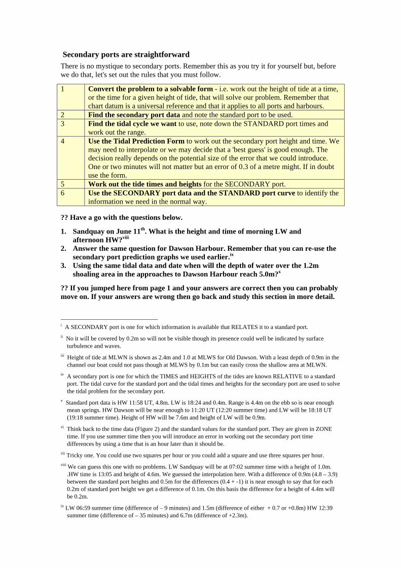
Secondary ports are straightforward There is no mystique to secondary ports. Remember this as you try it for yourself but, before we do that, let's set out the rules that you must follow.

1 Convert the problem to a solvable form - i.e. work out the height of tide at a time, or the time for a given height of tide, that will solve our problem. Remember that chart datum is a universal reference and that it applies to all ports and harbours.

2 Find the secondary port data and note the standard port to be used. 3 Find the tidal cycle we want to use, note down the STANDARD port times and

work out the range. 4 Use the Tidal Prediction Form to work out the secondary port height and time. We

may need to interpolate or we may decide that a 'best guess' is good enough. The decision really depends on the potential size of the error that we could introduce. One or two minutes will not matter but an error of 0.3 of a metre might. If in doubt use the form.

5 Work out the tide times and heights for the SECONDARY port. 6 Use the SECONDARY port data and the STANDARD port curve to identify the

information we need in the normal way.

?? Have a go with the questions below.

1. Sandquay on June 11th. What is the height and time of morning LW and afternoon HW?viii

2. Answer the same question for Dawson Harbour. Remember that you can re-use the secondary port prediction graphs we used earlier.ix

3. Using the same tidal data and date when will the depth of water over the 1.2m shoaling area in the approaches to Dawson Harbour reach 5.0m?x

?? If you jumped here from page 1 and your answers are correct then you can probably move on. If your answers are wrong then go back and study this section in more detail.

i A SECONDARY port is one for which information is available that RELATES it to a standard port. ii No it will be covered by 0.2m so will not be visible though its presence could well be indicated by surface

turbulence and waves. iii Height of tide at MLWN is shown as 2.4m and 1.0 at MLWS for Old Dawson. With a least depth of 0.9m in the

channel our boat could not pass though at MLWS by 0.1m but can easily cross the shallow area at MLWN. iv A secondary port is one for which the TIMES and HEIGHTS of the tides are known RELATIVE to a standard

port. The tidal curve for the standard port and the tidal times and heights for the secondary port are used to solve the tidal problem for the secondary port.

v Standard port data is HW 11:58 UT, 4.8m. LW is 18:24 and 0.4m. Range is 4.4m on the ebb so is near enough mean springs. HW Dawson will be near enough to 11:20 UT (12:20 summer time) and LW will be 18:18 UT (19:18 summer time). Height of HW will be 7.6m and height of LW will be 0.9m.

vi Think back to the time data (Figure 2) and the standard values for the standard port. They are given in ZONE time. If you use summer time then you will introduce an error in working out the secondary port time differences by using a time that is an hour later than it should be.

vii Tricky one. You could use two squares per hour or you could add a square and use three squares per hour. viii We can guess this one with no problems. LW Sandquay will be at 07:02 summer time with a height of 1.0m.

.HW time is 13:05 and height of 4.6m. We guessed the interpolation here. With a difference of 0.9m (4.8 – 3.9) between the standard port heights and 0.5m for the differences (0.4 + -1) it is near enough to say that for each 0.2m of standard port height we get a difference of 0.1m. On this basis the difference for a height of 4.4m will be 0.2m.

ix LW 06:59 summer time (difference of – 9 minutes) and 1.5m (difference of either + 0.7 or +0.8m) HW 12:39 summer time (difference of – 35 minutes) and 6.7m (difference of +2.3m).

x In working terms at HW –3h 20minutes or 09:19 summer time.