1

Chapter 1. Quantum Mechanics Notes: • Most of the material presented in this chapter is taken from Cohen-Tannoudji, Diu,

and Laloë, Chap. 3, and from Bunker and Jensen (2005), Chap. 2.

1.1 The Postulates of Quantum Mechanics

1.1.1 First Postulate

At a given time t , the physical state of a system is described by a ket ! t( ) (using Dirac’s notation). From this ket a wave function dependent on position and time can be defined by the projection onto a basis defined by the bra r . That is the wave function is given by ! r,t( ) " r ! t( ) . (1.1) The symbol is usually called a bracket. Equation (1.1) is the result of the following two definitions. First, the bracket is by definition a scalar product ! " # d 3x! * x( )" x( )$ . (1.2) Second, to the ket r is associated a Dirac distribution r !" x # r( ), (1.3) such that

r ! t( ) = d 3x" * x # r( )! x,t( )$

= d 3x" x # r( )! x,t( )$ =! r,t( ). (1.4)

Note that the “orthogonality” of the r kets is apparent from

!r r = d 3x" x # !r( )" x # r( )$

= " !r # r( ) d 3x" x # !r( )$ = " !r # r( ). (1.5)

2

1.1.2 Second Postulate

For every measurable physical quantity A corresponds an operator A , and this operator is an observable. It is often the case that a representation of kets and operators is done through vectors and matrices, respectively. The action of the operator on the ket produces a new ket ! = A " , (1.6) and this action is the mathematical equivalent of the multiplication of a vector and a matrix.

1.1.3 Third Postulate The outcome of the measurement of a physical quantity A must be an eigenvalue of the corresponding observable A . Since observables are related to physical quantities, then the matrix associated with them must be Hermitian. This is because the eigenvalues of Hermitian matrices are real quantities (in a mathematical sense). Recall that a matrix is Hermitian when Aij = Aji

* , (1.7) where * stands for complex conjugation. Alternatively, a Hermitian operator is one that is self-adjoint. That is, A† = A. (1.8) When the matrix is of finite dimension, then the eigenvalues are quantized (a “matrix” of infinite dimension would correspond to a continuum; for example, a matrix acting on r would have to be of infinite dimension as r encompasses the continuum made of all possible positions).

1.1.4 Fourth Postulate

The ket, say ! t( ) , specifying the state of a system is assumed normalized to unity. That is, ! t( ) ! t( ) = 1. (1.9) Alternatively, the associated wave function is also normalized, since ! t( ) ! t( ) = d 3x! * x,t( )! x,t( )" = d 3x ! x,t( ) 2" = 1. (1.10)

3

This ket can also be expanded using any suitable (complete) basis of kets. For example, using the r basis we have ! t( ) = d 3r c r,t( ) r" , (1.11) where c r,t( ) is the coefficient (it is actually the wave function itself, see equations (1.1) and (1.4)) resulting from the projection of ! t( ) on r . Equation (1.11) can therefore be written as ! t( ) = d 3r r ! t( )"# $% r& . (1.12) Rearranging this last equation we have ! t( ) = d 3r r r"#$ %

& ! t( ) , (1.13)

which implies that d 3r r r! = 1, (1.14) where 1 is the unit operator (or matrix). Similarly any other normalized ket ! that can

be expanded with a (complete) discrete and orthonormal basis ui (i.e., ui u j = ! ij ) with

! = ui !"# $% ui

i&

= ci uii& ,

(1.15)

is also normalized to unity, and we have the following relation for the basis ui ui

i! = 1. (1.16)

Equation (1.16) (as well as equation (1.14)) is a completeness relation that must be satisfied for the corresponding basis to be complete. In consideration of these facts and definitions, we can state the fourth postulate of quantum mechanics as follows: In measuring the physical quantity A on a system in the state ! , the probability of obtaining the (possibly degenerate) eigenvalue “a ” of the corresponding observable A is

4

P a( ) = un

i !2

i=1

gn

" , (1.17)

for discrete states, with gn the degree of degeneracy of “a ”, and un

i{ } the set of degenerate eigenvectors. For continuum states the corresponding probability is given by dP a( ) = va !

2da, (1.18)

where va is the eigenvector associated with the eigenvalue “a ”. We can apply this postulate to the case of a discrete degenerate state by starting with a generalization of equation (1.15)

! = cni un

i

i=1

gn

"n" . (1.19)

Projecting this state on the set of states um

j of degeneracy gm (i.e., j = 1,2,…,gm ), and taking the square of the norm we get

umj !

2

j=1

gm

" = cni um

j uni

i=1

gn

"n"

2

j=1

gm

"

= cni# ij#mn

i=1

gn

"n"

2

j=1

gm

"

= cmj 2

j=1

gm

" .

(1.20)

We, therefore, see that the probability of finding the system in a state (or group of states) possessing a given eigenvalue is proportional to the square of the coefficient cm

j that appears in the expansion defining the state in term of the basis under consideration (as is evident from equation (1.19)).

Alternatively, we define the projector Pn

Pn ! uni un

i

i=1

gn

" (1.21)

5

as the operator that projects a given state, say ! , on the subspace containing the set of

eigenvectors uni{ } that share the same eigenvalue. For example, using equation (1.21)

on ! we find

Pn ! = uni un

i !i=1

gn

" = cni un

i

i=1

gn

" , (1.22)

and it is clear from a comparison with equation (1.19) that the only part of ! that is left

is that corresponding to the subspace containing the eigenvectors uni{ } . For a

continuum of states, the projector is on the subspace va{ } corresponding to the domain of eigenvalues specified by a1 ! a ! a2 is P!a = va va daa1

a2" . (1.23)

1.1.5 Fifth Postulate

If the measurement of the physical quantity A on a system in the state ! gave the value “ a ” as a result, then state of the system immediately following the measurement is given by the new state !" such that (for discrete states)

!" =Pn "

" Pn ". (1.24)

This postulate simply ensures that the new ket (or wave function) describing the system after a measurement is suitably normalized to unity. Indeed, we can verify from equations (1.19) and (1.21) that

!" =uni un

i "i=1

gn

#

" uni un

i "i=1

gn

#=

cni un

i

i

gn

#

cni 2

i=1

gn

#, (1.25)

and therefore

6

!" !" =unj cn

j( )*j=1

gn

# $ cni un

i

i

gn

#

cni 2

i=1

gn

#=

cnj( )* cni% ij

i=1

gn

#j=1

gn

#

cni 2

i=1

gn

#

=cni 2

i=1

gn

#

cni 2

i=1

gn

#= 1.

(1.26)

1.1.6 Sixth Postulate Although it is possible to give a “derivation” of Schrödinger’s equation, it is sufficient for our purposes to introduce it as the sixth, and last, postulate of quantum mechanics: The time evolution of the state vector ! t( ) of a system is dictated by the Schrödinger equation

i!ddt

! t( ) = H t( ) ! t( ) , (1.27)

where H t( ) is the Hamiltonian of the system, i.e., the observable associated with the energy of the system. In most cases, we will be dealing with a time-independent Hamiltonian that has so-called stationary states whose norms do not change as a function of time. More precisely, consider the following ket ! t( ) = e" iEt ! # , (1.28) where E is the energy associated with the state. It is clear that ! t( ) ! t( ) = " " , (1.29) and if we insert equation (1.28) into Schrödinger equation (i.e., (1.27)), then find that H ! = E ! (1.30)

Therefore, the energy E is the eigenvalue of the Hamiltonian H for the stationary state ! . Equation (1.30) is often referred to as the time-independent Schrödinger equation.

7

It is important to note that since the observables R and P associated with the position and the momentum, respectively, do not commute (i.e., R ! P " P ! R ) and that they usually appear in expressions for the Hamiltonian, rules of symmetry must be used when dealing with their products. For example, the following transformation would be applied for the simple product R ! P

R ! P" 12R ! P + P ! R( ). (1.31)

1.2 Important Operators and Commutation Relations Two measurable physical quantities that are included in the expression for the classical Hamiltonian are the position r and the momentum p vectors. Correspondingly, it is necessary to introduce the aforementioned operators R and P when setting up the quantum mechanical Hamiltonian. These two operators can be broken down into the usual three components

R = Xex + Yey + ZezP = Pxex + Pyey + Pzez .

(1.32)

The complete basis r{ } contains the eigenvectors for R . More precisely, we can write r = x y z , (1.33) and X x = x x (1.34) or X r = x r . (1.35) Similar relations hold for Y and Z . We can also define a complete basis p{ } of eigenvectors for the momentum operator such that

p = px py pz

Px px = px pxPx p = px p ,

(1.36)

8

and so on. The question is: what is the representation for P when acting on the r{ } (or

that of R for p{ } )? To answer this question we first note that the momentum basis satisfies relations that are similar to that satisfied by the position basis. That is,

p0 !" p # p0( )p $p = " p # $p( )

d 3p p p% = 1

p & =& p( ).

(1.37)

We now combine the second of these relations (i.e., the one concerning the orthogonality of the momentum kets) and equation (1.14) for the completeness of the r{ } basis

p !p = d 3r p r r !p"= d 3r v* r;p( )v r; !p( )"= # p $ !p( ),

(1.38)

where v r;p( ) ! r p and is to be determined. Alternatively, we can combine equation (1.5) and the third of equations (1.37) and get

r !r = d 3p r p p !r"= d 3p v r;p( )v* !r ;p( )"= # r $ !r( ).

(1.39)

We can consider equations (1.38) and (1.39) as the relations that define v r;p( ) . One form that satisfy these conditions is

v r;p( ) = 1

2!!( )3 2eip"r ! , (1.40)

where ! is some constant having the dimension of angular momentum, and we identify it with Planck’s constant (divided by 2! ). [Note: The fact that equation (1.40) satisfies both equations (1.38) and (1.39), can be verified by considering the Fourier transform pair between a function f r( ) and its transform f p( )

9

f r( ) = 12!!( )3 2

d 3p f p( )eip"r !#

f p( ) = 12!!( )3 2

d 3r f r( )e$ ip"r !# . (1.41)

Equations (1.41) imply the following duality between the Fourier transform and its inverse

f r( )! f p( )

f "r( )! f p( ). (1.42)

For example, if we set f r( ) = ! r " #r( ) , then it is easy to show that

f p( ) = 1

2!!( )3 2d 3r" r # $r( )e# ip%r !& =

12!!( )3 2

e# ip% $r ! . (1.43)

Therefore, from the second of equations (1.42) we have

! p " #p( ) = 1

2$!( )3 2d 3r 1

2$!( )3 2eir % #p !&

'((

)

*++e" ip%r !, , (1.44)

which is the same as equation (1.38) when v r;p( ) is given by equation (1.40). Similarly, we can first set f p( ) = ! p + "p( ) to get

f r( ) = 1

2!!( )3 2d 3p" p + #p( )eip$r !% =

12!!( )3 2

e& i #p $r ! , (1.45)

and from the first of equations (1.42) we have

! "r + #r( ) = ! r " #r( ) = 1

2$!( )3 2d 3r 1

2$!( )3 2e" i #r %p !&

'((

)

*++eip%r !, , (1.46)

which is the same as equation (1.39).] Having established that

r p =

12!!( )3 2

eip"r ! , (1.47)

10

consider equation (1.1) while using the completeness relation for p{ } (i.e., the third of equations (1.37))

! r,t( ) = r ! t( ) = d 3p r p" p ! t( )

=1

2#!( )3 2d 3peip$r !" ! p, t( ).

(1.48)

It is therefore apparent from this last equation that the two different forms of the wave function are related through the Fourier transform ! r,t( )"! p, t( ). (1.49) Finally, consider the action of the momentum operator on the ket ! t( ) with

r P! t( ) = d 3p r P p p ! t( )"= d 3pp r p ! p, t( )" =

12#!( )3 2

d 3peip$r !p! p, t( )"

= %i!& 12#!( )3 2

d 3peip$r !! p, t( )"'

())

*

+,,

= %i!& r ! t( ) .

(1.50)

We therefore find the fundamental result that the action of the momentum operator in the position basis r{ } is represented by P!"i!# (1.51) In quantum mechanics the order with which measurements are made can be important. For example, the act of measuring the momentum of a system can affect its position, and vice-versa. It is therefore interesting to calculate the difference between two sets of measurements. Consider the following ! = RP " PR( ) # , (1.52) the ket resulting from the difference between measuring the momentum before the position on a system ! and measuring the position before the momentum. To proceed further, we project both sides of equation (1.52) on r , and use equation (1.51) to get

11

r ! = r RP " PR( )# = r r P# " r P R #( )= "i! r$ r # " $ r R #%

&'( = "i! r$ r # " $ r r #( )%& '(

= "i! r$ r # " 1 r # " r$ r #%& '( = i!1 r # .

(1.53)

We, therefore, find the following important result

R, P!" #$ % RP & PR = i!1, (1.54)

or alternatively

Rj , Pk!" #$ = i!% jk (1.55)

where R, P!" #$ is the commutator of R and P . It should also be obvious that Rj , Rk!" #$ = Pj , Pk!" #$ = 0. (1.56) Another fundamental operator is that of the angular momentum L = R ! P, (1.57) which has the following commutation properties (Einstein’s summation convention adopted)

Rj , Lk!" #$ = %klm Rj , Rl Pm!" #$ = %klm Rl Rj , Pm!" #$ + Rj , Rl!" #$ Pm{ }= %klm Rl i!& jm( ) = i!% jkl Rl

Pj , Lk!" #$ = %klm Pj , Rl!" #$ Pm = %klm 'i!& jl( ) Pm = i!% jkl Pl ,

(1.58)

and

L j , Lk!" #$ = % jmn RmPn , Lk!" #$ = % jmn Rm Pn , Lk!" #$ + Rm , Lk!" #$ Pn{ }= i!% jmn %nkl RmPl + %mkl Rl Pn{ }= i! & jk&ml ' & jl&mk( ) RmPl + &nk& jl ' &nl& jk( ) Rl Pn{ }= i! Rj Pk ' Rk Pj( ),

(1.59)

where we used !njm!nkl = " jk"ml # " jl"mk . The last equation can also be written as

12

L j , Lk!" #$ = i!% jkl Ll (1.60)

If we consider the square of the total angular momentum L2 = L j L j , then we have

L2 , Lk!" #$ = L j L j , Lk!" #$ + L j , Lk!" #$ L j

= i!% jkl L j Ll & L j Ll( ) = 0 (1.61)

and

L2 , Rj!" #$ = Lk Lk , Rj!" #$ + Lk , Rj!" #$ Lk = %i!& jkl Lk Rl + Rl Lk( )= %i!& jkl 2Rl Lk % i!&lkm Rm( ) = 2 i!& jkl Rk Ll + !

2Rj( )L2 , Pj!" #$ = 2 i!& jkl Pk Ll + !

2Pj( ). (1.62)

That is to say, any component of the angular momentum operator commutes with the square of the total angular momentum. On the other hand, the components of the position and momentum operators do not commute with the components, or the square, of the angular momentum. However, a little more work will show that

L2 , Ri Rj!" #$ = 2!2 R2% ij & 3Ri Rj( )

L2 , PiPj!" #$ = 2!2 P2% ij & 3PiPj( ),

(1.63)

and most notably (using also equations (1.58)) Lk , R

2!" #$ = Lk , P2!" #$ = L2 , R2!" #$ = L2 , P2!" #$ = 0. (1.64)

It is important to note that other operators (e.g., F, I , J, N , and S ) to be introduced later are also used to represent other angular momenta and spins.

1.3 Heisenberg Inequality Whenever two observables Q and P satisfy the same commutation relation as the position and momentum operators, i.e.,

Q, P!" #$ = i!, (1.65)

then we say that they are conjugate operators. Let’s assume that for both operators

13

Q = ! Q ! = 0

P = ! P ! = 0. (1.66)

This is not a restriction, since we could always define new operators by subtracting Q and P from Q and P , respectively, in the event that they weren’t null. Now consider the following quantity I = ! Q2 ! ! P2 ! . (1.67)

If we define new states such that

1 ! Q "

2 ! P " , (1.68)

then using the Schwarz Inequality we can write I = 11 2 2 ! 1 2 2 1 , (1.69) since 1 2 is a scalar product. We can rewrite the last part of this inequality as follows

1 2 2 1 =14

1 2 + 2 1( )2 ! 1 2 ! 2 1( )2"#

$%

=14

& QP & + & PQ &( )2 ! & QP & ! & PQ &( )2"#'

$%(

=14

& QP + PQ &( )2 ! & QP ! PQ &( )2"#'

$%(

=14

& Q, P{ }&( )2 ! & Q, P"# $% &( )2"#'

$%(.

(1.70)

The quantity Q, P{ } ! QP + PQ is commonly called the anti-commutator, for obvious reasons. We should note that

! Q, P{ }!( )2 = ! Q, P{ }! 2

" 0, (1.71)

since ! Q, P{ }! = ! Q, P{ }! * because Q and P are observables (i.e., Hermitian

operators). Taking this result into account, we can now insert equation (1.65) into equation (1.70) and find

14

! Q2 ! ! P2 ! "

!2

4 (1.72)

This last equation is a generalization of the so-called Heisenberg inequality, which is usually written as follows

!Q " !P #

!2, (1.73)

with

!Q " # Q2 #

!P " # P2 # . (1.74)

1.4 Diagonalizing the Hamiltonian Matrix Given a basis ! i{ } , the elements of the Hamiltonian are calculated with Hij = ! i H ! j . (1.75)

It is straightforward to verify this equation with column and row vectors for the basis, and a matrix for the Hamiltonian. Using the position basis and its completeness relation we can express equation (1.75) with the wave functions that correspond to the basis

Hij = ! i H ! j = d 3r" ! i r r H ! j

= d 3r" ! i* r( ) H! j r( ),

(1.76)

where in the last expression it is implied that the Hamiltonian is expressed using its representation in the position basis. For example, for a free particle of mass m whose classical Hamiltonian is

H =p2

2m, (1.77)

the corresponding quantum mechanical Hamiltonian operator in the last expression of equation (1.76) is

15

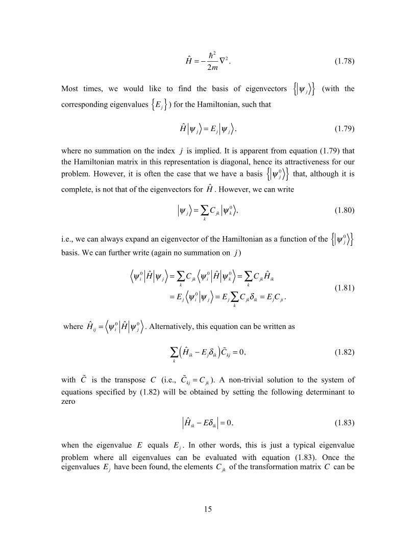
H = !

!2

2m"2 . (1.78)

Most times, we would like to find the basis of eigenvectors ! j{ } (with the

corresponding eigenvalues Ej{ } ) for the Hamiltonian, such that H ! j = Ej ! j , (1.79) where no summation on the index j is implied. It is apparent from equation (1.79) that the Hamiltonian matrix in this representation is diagonal, hence its attractiveness for our problem. However, it is often the case that we have a basis ! j

0{ } that, although it is

complete, is not that of the eigenvectors for H . However, we can write ! j = Cjk ! k

0

k" , (1.80)

i.e., we can always expand an eigenvector of the Hamiltonian as a function of the ! j

0{ }

basis. We can further write (again no summation on j )

! i

0 H ! j = Cjk ! i0 H ! k

0

k" = Cjk Hik

k"

= Ej ! i0 ! j = Ej Cjk# ik

k" = EjCji .

(1.81)

where Hij = ! i

0 H ! j0 . Alternatively, this equation can be written as

Hik ! Ej" ik( ) !Ckj

k# = 0, (1.82)

with !C is the transpose C (i.e.,

!Ckj = Cjk ). A non-trivial solution to the system of equations specified by (1.82) will be obtained by setting the following determinant to zero Hik ! E" ik = 0, (1.83) when the eigenvalue E equals Ej . In other words, this is just a typical eigenvalue problem where all eigenvalues can be evaluated with equation (1.83). Once the eigenvalues Ej have been found, the elements Cjk of the transformation matrix C can be

16

calculated with equation (1.82). But the orthonormality condition for the basis ! j{ }

implies that

! j ! k = ! m

0 Cjm* Ckn ! n

0

n"

m" = Cjm

* Ckn ! m0 ! n

0

m,n" = Cjm

* Ckn#mnm,n"

= Cjm* Ckm

m" = # jk .

(1.84)

This last equation implies that the transformation matrix is unitary, that is C† = C!1. (1.85) If we introduce the diagonal matrix ! whose elements are the eigenvalues Ej (i.e., !ij = Ei" ij , no implied summation), then from equations (1.82) and (1.85) we can write (with H the Hamiltonian matrix) H !C = !C!, (1.86) or alternatively !C!1H !C = ". (1.87) Example We consider the case of a two-level system with the corresponding two-dimensional Hamiltonian matrix

H =E10 H12

H12* E2

0

!

"#

$

%&, (1.88)

where E1

0 and E20 are the eigenvalues of the unperturbed kets ! 1

0 and ! 20 .

Straightforward application of equation (1.83) for the determination of the eigenvalues of the Hamiltonian yields E1

0 ! E( ) E20 ! E( ) ! H122 = E2 ! E1

0 + E20( )E ! H12

2 ! E10E2

0( ) = 0, (1.89)

with the following roots

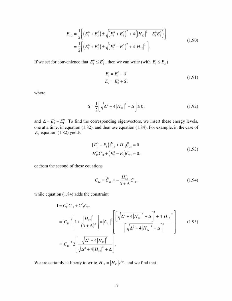
17

E1,2 =

12

E10 + E2

0( ) ± E10 + E2

0( )2 + 4 H122 ! E1

0E20( )"

#$%&'

=12

E10 + E2

0( ) ± E20 ! E1

0( )2 + 4 H122"

#$%&'.

(1.90)

If we set for convenience that E1

0 ! E20 , then we can write (with E1 ! E2 )

E1 = E1

0 ! SE2 = E2

0 + S, (1.91)

where

S =12

!2 + 4 H122 " !#

$%&'() 0, (1.92)

and ! = E2

0 " E10 . To find the corresponding eigenvectors, we insert these energy levels,

one at a time, in equation (1.82), and then use equation (1.84). For example, in the case of E1 equation (1.82) yields

E10 ! E1( ) !C11 + H12

!C21 = 0

H12* !C11 + E2

0 ! E1( ) !C21 = 0, (1.93)

or from the second of these equations

C12 = !C21 = !

H12*

S + "C11, (1.94)

while equation (1.84) adds the constraint

1 = C11*C11 + C12

* C12

= C112 1+

H122

S + !( )2"

#$$

%

&''= C11

2!2 + 4 H12

2 + !"#$

%&'

2

+ 4 H122

!2 + 4 H122 + !"

#$%&'

2

"

#

$$$$

%

&

''''

= C112 2

!2 + 4 H122

!2 + 4 H122 + !

"

#

$$

%

&

''.

(1.95)

We are certainly at liberty to write H12 = H12 e

i! , and we find that

18

C+ ! C11 =121+ "

"2 + 4 H122

#

$

%%

&

'

((

1 2

C) ! )C12* = ei* 1) C11

2 =ei*

21) "

"2 + 4 H122

#

$

%%

&

'

((

1 2

,

(1.96)

where the sign and phase of C12 are dictated by that of H12 through equation (1.94). A similar exercise for E2 can be shown to yield C22 = C11 = C+ and C21 = !C12

* = C! . The eigenvectors are thus given by

! 1 = C+ ! 1

0 " C"* ! 2

0

! 2 = C+ ! 20 + C" ! 1

0 . (1.97)

It is straightforward to verify that equation (1.86) is satisfied with the transformation matrix defined with equations (1.96) and (1.97). Let’s now concentrate on cases where H12 is real and small, i.e., H12

* = H12 ! ! . We can then calculate the following approximations

S =12

!2 + 4H122 " !#

$%& !

12

! 1+ 2H122

!2

'()

*+," !

#

$-

%

&.

!H12

2

!

C+ =121+ !

!2 + 4H122

#

$--

%

&..

1 2

!121+ 1" 2H12

2

!2

'()

*+,

#

$-

%

&.

1 2

! 1" H122

2!2

C" =121" !

!2 + 4H122

#

$--

%

&..

1 2

!121" 1" 2H12

2

!2

'()

*+,

#

$-

%

&.

1 2

!H12

!.

(1.98)

We see that the amount by which the states ! 1

0 and ! 20 mix to form the new

eigenvectors is a function of both H12 and ! . The smaller their ratio (i.e., H12 ! ) the more the states and energies of the true Hamiltonian resemble that of the unperturbed two-level system. It is also apparent that the perturbation has for effect to increase the energy difference between the two levels.

19

1.5 The Classical Molecular Hamiltonian To set up the quantum mechanical Hamiltonian for a molecule, we first write down the classical Hamiltonian and then make the appropriate coordinates changes before expressing the corresponding relation with the proper quantum mechanical operators. For a molecule made of a total of l particles, with N nuclei and l ! N electrons, the total energy is given by the sum of the kinetic and potential energies T and V , respectively. These two quantities are given by (using Système International units)

T = 12

mr!Xr2 + !Yr

2 + !Zr2( )

r=1

l

!

V = 14"#0

CrCse2

Rrsr<s=1

l

! , (1.99)

where, for the r th particle, mr is the mass, the position is specified by Xr ,Yr , and Zr and measured from some arbitrary space-fixed coordinate system, Cre is the charge, and Rrs

Rrs = Xr ! Xs( )2 + Yr ! Ys( )2 + Zr ! Zs( )2 (1.100) is the distance to particle s . Finally, !0 is the permittivity of vacuum. We know that the kinetic energy can be decomposed into two components: one (TCM ) due to the motion of the centre of mass of the system, and another (Trve ) arising from the motions of the nuclei and electrons relative to the centre of mass. To separate these two terms, we introduce Xr ,Yr , and Zr the position components of the r th particle relative to the centre of mass located at X0,Y0, and Z0 such that

Xr = Xr + X0

Yr = Yr + Y0Zr = Zr + Z0.

(1.101)

Obviously, Rrs is unchanged in quantity by the introduction of these new variables, but only in form with

Rrs = Xr ! Xs( )2 + Yr !Ys( )2 + Zr ! Zs( )2 . (1.102) On the other hand, if we write the sum of the kinetic energies from particles r = 2,…,l as a function of X0,Y0,Z0,X2 ,Y2 ,Z2 ,…,Xl ,Yl ,Zl and the associated velocities, we find that

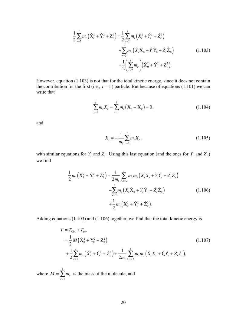
20

12

mr!Xr2 + !Yr

2 + !Zr2( )

r=2

l

! = 12

mr!Xr2 + !Yr

2 + !Zr2( )

r=2

l

!

+ mr!Xr!X0 + !Yr !Y0 + !Zr

!Z0( )r=2

l

!

+ 12

mrr=2

l

!"#$%&'!X02 + !Y0

2 + !Z02( ).

(1.103)

However, equation (1.103) is not that for the total kinetic energy, since it does not contain the contribution for the first (i.e., r = 1 ) particle. But because of equations (1.101) we can write that

mrXrr=1

l

! = mr Xr " X0( )r=1

l

! = 0, (1.104)

and

X1 = !1m1

mrXrr=2

l

" , (1.105)

with similar equations for Y1 and Z1 . Using this last equation (and the ones for Y1 and Z1 ) we find

12m1!X12 + !Y1

2 + !Z12( ) = 1

2m1

mrms!Xr!Xs + !Yr !Ys + !Zr

!Zs( )r ,s=2

l

!

" mr!Xr!X0 + !Yr !Y0 + !Zr

!Z0( )r=2

l

!

+12m1!X02 + !Y0

2 + !Z02( ).

(1.106)

Adding equations (1.103) and (1.106) together, we find that the total kinetic energy is

T = TCM + Trve

=12M !X0

2 + !Y02 + !Z0

2( )

+12

mr!Xr2 + !Yr

2 + !Zr2( )

r=2

l

! +12m1

mrms!Xr!Xs + !Yr !Ys + !Zr

!Zs( )r ,s=2

l

! ,

(1.107)

where M = mrr=1

l

! is the mass of the molecule, and

21

TCM =12M !X0

2 + !Y02 + !Z0

2( )

Trve =12

mr!Xr2 + !Yr

2 + !Zr2( )

r=2

l

! +12m1

mrms!Xr!Xs + !Yr !Ys + !Zr

!Zs( )r ,s=2

l

! . (1.108)

The index “rve” stands for rovibronic (rotation-vibration-electronic), and is associated with the internal kinetic energy of the molecule, as opposed to the external or translational kinetic energy. We see from equations (1.108) that we have, as expected, a complete separation of the translational and internal components of the energy. As far as we are concerned, we will not worry about the translational kinetic energy associated with the centre of mass of the molecule, and only use the rovibronic part of the energy Erve when dealing with problems in molecular spectroscopy. More specifically, we have Etotal = TCM + Erve , (1.109) with

Erve = Trve +V

=12

mr!Xr2 + !Yr

2 + !Zr2( )

r=2

l

! +12m1

mrms!Xr!Xs + !Yr !Ys + !Zr

!Zs( )r ,s=2

l

!

+14"#0

CrCse2

Rrsr<s=1

l

! .

(1.110)

The rovibronic energy is the quantity that we need to consider to determine the spectroscopy of a molecule.

1.6 The Quantum Mechanical Rovibronic Hamiltonian To convert the classical rovibronic energy Erve into the needed quantum mechanical version of the Hamiltonian, we must first express equation (1.110) as a function of the coordinates Xr ,Yr , and Zr and momenta PXr ,PYr , and PZr . We could then replace these quantities with the corresponding quantum mechanical operators (see equations (1.32) and (1.51)) and obtain an expression for the quantum mechanical Hamiltonian. To accomplish our first aforementioned task, we make use of the Lagrangian definition for the momenta, i.e.,

PXr =

!Lrve! !Xr

,…, (1.111)

where Lrve ! Trve "V is the (rovibronic) Lagrangian. In this case, since the potential energy is not a function of the velocities, then equation (1.111) simplifies to

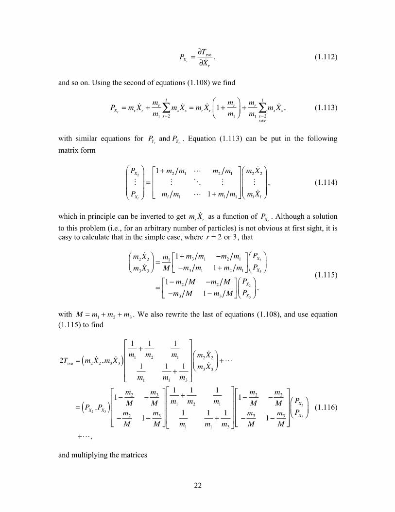
22

PXr =

!Trve! !Xr

, (1.112)

and so on. Using the second of equations (1.108) we find

PXr = mr!Xr +

mr

m1

ms!Xs

s=2

l

! = mr!Xr 1+

mr

m1

"#$

%&'+mr

m1

ms!Xs

s=2s( r

l

! , (1.113)

with similar equations for PYr and PZr . Equation (1.113) can be put in the following matrix form

PX2!PXl

!

"

###

$

%

&&&=1+ m2 m1 " m2 m1

! # !ml m1 " 1+ ml m1

'

(

)))

*

+

,,,

m2$X2!

ml$Xl

!

"

###

$

%

&&&, (1.114)

which in principle can be inverted to get mr

!Xr as a function of PXr . Although a solution to this problem (i.e., for an arbitrary number of particles) is not obvious at first sight, it is easy to calculate that in the simple case, where r = 2 or 3 , that

m2!X2

m3!X3

!"#

$%&=m1

M1+ m3 m1 'm2 m1

'm3 m1 1+ m2 m1

(

)*

+

,-PX2PX3

!"#

$%&

=1' m2 M 'm2 M'm3 M 1' m3 M

(

)*

+

,-PX2PX3

!"#

$%&,

(1.115)

with M = m1 + m2 + m3 . We also rewrite the last of equations (1.108), and use equation (1.115) to find

2Trve = m2!X2 ,m3

!X3( )1m1

+1m2

1m1

1m1

1m1

+1m3

!

"

####

$

%

&&&&

m2!X2

m3!X3

'()

*+,+"

= PX2 ,PX3( )1- m2

M-m3

M

-m2

M1- m3

M

!

"

####

$

%

&&&&

1m1

+1m2

1m1

1m1

1m1

+1m3

!

"

####

$

%

&&&&

1- m2

M-m2

M

-m3

M1- m3

M

!

"

####

$

%

&&&&

PX2PX3

'()

*+,

+",

(1.116)

and multiplying the matrices

23

2Trve = PX2 ,PX3( )1! m2

M!m3

M

!m2

M1! m3

M

"

#

$$$$

%

&

''''

1m2

0

0 1m3

"

#

$$$$

%

&

''''

PX2PX3

()*

+,-+!

= PX2 ,PX3( )1m2

!1M

!1M

!1M

1m3

!1M

"

#

$$$$

%

&

''''

PX2PX3

()*

+,-+!,

(1.117)

or

Trve =12mr

PXr2 + PYr

2 + PZr2( )

r=2

3

! "12M

PXr PXs + PYr PYs + PZr PZs( )r ,s=2

3

! . (1.118)

Although we limited ourselves to only three particles in the preceding example, we will take it on faith that this result can be extended to an arbitrary number of particles (it can be), and write

Erve =

12mr

PXr2 + PYr

2 + PZr2( )

r=2

l

! "12M

PXr PXs + PYr PYs + PZr PZs( )r ,s=2

l

!

+14#$0

CrCse2

Rrsr<s=1

l

! , (1.119)

for the rovibronic energy of a molecule. We are now in a position to write down the equation for the quantum mechanical rovibronic Hamiltonian. Using equations (1.51) and (1.119) we have

H rve = !!2

12mr

"r2 +!2

2M"r #"s

r ,s=2

l

$r=2

l

$ +14%&0

CrCse2

Rrsr<s=1

l

$ (1.120)

with

!r = eX""Xr

+ eY""Yr

+ eZ""Zr

, (1.121)

as a representation in the usual coordinate space.

24

1.7 The Rovibronic Schrödinger Equation To the rovibronic Hamiltonian of equation (1.120) will correspond eigenfunctions !rve such that H rve!rve X2 ,Y2 ,Z2 ,…,Xl ,Yl ,Zl( ) = Erve!rve X2 ,Y2 ,Z2 ,…,Xl ,Yl ,Zl( ), (1.122) where Erve is now an eigenvalue of the Hamiltonian. It is possible to show (using equations (1.64) and (1.105)) that the rovibronic Hamiltonian commutes with the total orbital angular momentum and its square, and thus share the same set of eigenfunctions with these operators. More precisely, defining J 2 and JZ for the operators of the square and the Z-component of the total orbital angular momentum, respectively, we have

H rve!rve = Erve!rve

J 2!rve = J J +1( )!2!rve , J = 0,1,2,…

JZ!rve = m!!rve , m = 0,1,2,…, J

(1.123)

where J and m are the so-called total orbital angular momentum and projection quantum numbers, respectively.

1.7.1 The Fine Structure and Hyperfine Structure Hamiltonians The rovibronic Hamiltonian of equation (1.120) does not take into account some interactions due to the intrinsic magnetic moment (i.e., spin) of the electrons, and the intrinsic magnetic and electric moments of the nuclei. More precisely, if we only consider the individual electron spins si , and the so-called electron spin-spin and spin-orbit couplings, then the electron fine structure Hamiltonian H es must be introduced

H es !14!"0

#emec

$%&

'()

21Rij3 Ri # R j( ) * Pi

2# Pj

$

%&'

()+

,--

.

/001 si

j2 i3

456

76

+e

mec2

C8eRi83 Ri # R8( ) * Pi

2me

#P8m8

$

%&'

()+

,--

.

/001 si

8 ,i3

+emec

$%&

'()

21Rij3 si 1 s j #

3Rij2 si 1 Ri # R j( )+,

./ s j 1 Ri # R j( )+,

./

$

%&'

()+

,--j>i

3

#8!39 Ri # R j( ) si 1 s j( ).

/0:;<,

(1.124)

where ! labels the nuclei, and i and j label the electrons. In equation (1.124), the first term (a spin-orbit interaction) corresponds to the coupling of the spin of each electron to the magnetic field it feels (in its reference frame) because of the presence of the electric

25

Coulomb fields due to the other electrons (in their respective reference frames). The second term is also a spin-orbit interaction but this time with the Coulomb field of the nuclei, and the last term corresponds the spin-spin couplings between the intrinsic magnetic moments of each pair of electrons. The internal molecular Hamiltonian then becomes H int = H rve + H es , and the total angular momentum must include both the orbital and electron spin momenta. It is usual to denote the orbital angular momentum with N (instead of J ), and the total angular momentum with J . We then write J = N + S, (1.125) where S is the total electron spin operator. The associated quantum numbers J and m refer to the sum of the orbital and spin angular momenta, and are those with which the molecular eigenfunctions can be labeled. On the other hand, if the interactions of the intrinsic magnetic and electric moments of the nuclei are taken into account, then the total angular momentum is denoted by F with F = J + I = N + S + I, (1.126) where I is the total nuclear spin angular momentum. The corresponding nuclear hyperfine structure Hamiltonian Hhfs will include nuclei spin interactions similar in form to those of equation (1.124), as well as terms due to the nuclei electric quadrupole fields. The internal molecular Hamiltonian then becomes H int = H rve + H es + Hhfs , (1.127) and the good quantum numbers with which the associated eigenfunctions can be labeled are those corresponding to F2 and FZ , i.e., F and mF ( mF = 0,1,2,…,F ).