1

CHAPTER 1

INTRODUCTION

1.1 GROUNDWATER

Groundwater is a distinguished component of the hydrologic cycle.

Groundwater is the water which occupies the voids in the saturated zone of

earth’s crust (rocks). It moves and stores in pore space (voids) of sedimentary

rocks or in the fractures and joints of hard rocks. The uncertainty about the

occurrence, distribution and quality aspect of groundwater and the energy

requirement for its withdrawal impose restriction on exploitation of

groundwater. In spite of its uncertainty, groundwater is much protected from

pollution; it requires little treatment before it use; it is available almost

everywhere; it can be developed with little gestation period and can be

supplied at a fairly steady rate.

1.2 GROUNDWATER SITUATION IN INDIA

India is a vast country having diversified geological setting.

Variations exhibited by the rock formations, ranging in age from the Archaean

crystalline to the recent alluvia, are as great as the hydrometeorological

conditions. The land forms vary from sea level at the coasts to the lofty peaks

of snow clad Himalayan Mountains attaining staggering altitude upto about

9000 metres. Variations in the nature and composition of rock types, the

geological structures, geomorphological set up and hydrometeorological

conditions have correspondingly given rise to widely varying groundwater

situation in different parts of the country.

2

Groundwater plays an important role in augmenting water supply to

meet the ever increasing demands for various domestic, agricultural and

industrial uses. It is the only source of drinking water for about 90% of Indian

population. The rapid growth rates of population, industry and agricultural

practice have not only increased the exploitation of groundwater but have also

contributed towards the deterioration of its quality. Therefore, the preservation

and improvement of groundwater quality is of vital importance for human well

being as well as for the sustainability of clean environment.

1.3 GROUNDWATER POLLUTION

Sources of groundwater pollution can be classified mainly into two

groups. These are anthropogenic (or man made) sources and natural sources.

Anthropogenic sources include industrial wastes, municipal wastes, fertilizers,

pesticides etc. Natural sources are mainly hazardous substances such as

arsenic, fluoride, nitrates, carbonates, trace elements etc. present in the host

geological formations. Some times natural sources are also activated by human

interference with the groundwater system such as pumping of groundwater in

excess to natural replenishment of aquifers which disturbs the regional water

balance which is otherwise in the equilibrium state. It may lead to the pollution

of fresh water due to encroachment of polluted water from the surrounding

polluted groundwater resources. Groundwater moves very slowly on the order

of 1 cm per day, so it takes a long time for contaminants to reach a drinking

water aquifer. The residence time of the water in the surficial aquifer is likely

to be on the order of decades, and deep aquifer water are thousands of years

old. So the good news is that it takes a long time to pollute an aquifer, but the

bad news is that once the aquifer is contaminated, it will probably take a very

long time for natural restoration.

3

1.4 BACKGROUND OF THE RESEARCH PROBLEM

1.4.1 Amaravathi River

The Amaravathi river is a tributary of river Cauvery, South India.

The 175 km long Amaravathi river begins at the Kerala / Tamil Nadu State

border at the bottom of Manjampatti valley between the Annamalai Hills and

the Palani Hills. It descends in a north eastern direction through Amaravathi

reservoir and Amaravathi dam at Amaravathinagar. It is joined by Kallapuram

river at the mouth of the Ajanda valley in Udumalaipettai of Coimbatore

district and Nanganji river near Aravakurichi and Kodaganar river near

Kodaiyur. Finally Amaravathi river joins with river Cauvery at Kattali near

Karur. The river irrigates over 60,000 acres (240 km2) of agricultural lands of

in Coimbatore, Erode and Karur districts. The Amaravathi river and its basin,

especially in the vicinity of Karur are heavily used for drawing water for

industrial process and for the disposal of wastewater. As a result the river and

the groundwater in the basin are severely polluted.

1.4.2 Amaravathi River Basin in Karur District

Amaravathi river basin is located between north latitude 11o00' N

and 10o00'N, east longitude 77

o00'E and 78

o15'E. The Amaravathi river enters

into Karur district near Chinnadarapuram (30km upstream of Karur) and

merges with river Cauvery near Kattali village (10 Km down stream of Karur).

The flow in the river is seasonal and is contributed by the northeast and

southwest monsoon seasons. Amaravathi river is the main source of water for

domestic, irrigation and industrial uses in Karur district. Till the river reaches

Karur, it is free from pollution. Whereas the river is severely polluted in Karur

due to the discharge of partially treated effluent from the textile bleaching and

dyeing units located in and around Karur Town. The TDS level in

4

groundwater quality is getting increased. Agricultural production is in the

down trend. Farmers are seeking compensation.

1.5 NEED FOR THE STUDY

Karur is the head quarter of Karur taluk and district. It is located on

the bank of river Amaravathi (Figure 1.1). During the last three decades the

town emerged as a major textile centres with more than 1000 power loom and

handloom units producing bed spreads, towels and furnishings. The main raw

material is cotton yarn. This cotton yarn and the finished product (i.e) gray

cloth are bleached any dyed by the industries located in this town. At present

487 bleaching and dyeing units are in operation. These bleaching and dyeing

units are located on either side of Amaravathi river within 2Km from the river

bank and total of 10 km stretch on either side of Karur. By average one unit

generates 30 kilo litres per day (KLD) of trade effluent. These units have

provided either individual effluent treatment plant (IETP) or joined in common

effluent treatment plant (CETP). After treatment the effluent is discharged into

river Amaravathi. The total dissolve solids (TDS) in the river discharge is in

the range of 5000 – 10000 mg/L and the chloride is in the range of 2000 –

4000 mg/L. Daily 14600 KLD of partially treated effluent is discharged into

the river. On average daily 90.89 tonnes of TDS with 49.94 tonnes of chlorides

are let into river. This salt ultimately accumulates in the soil and increase the

TDS level in the groundwater. The effluent reaching the river is dark brown in

colour. During summer period there is no water flow in river, only effluent

flow can be noticed. In monsoon period the colour in river water can be

noticed upto Kattali where the river get confluence with river Cauvery.

Hence a detailed study on the impact of industrial effluent on the groundwater

quality in this area is highly needed.

5

Figure 1.1 Location of Study Area

Figure 1.2 Amaravathi River Basin Figure 1.3 Google Map of Karur &

Amaravathi River

1.6 OBJECTIVES AND SCOPE OF THE RESEARCH

The farmers of Amaravathi Ayacut had filed a writ petition in the

High Court of Madras seeking compensation for damage caused to their crops,

6

lands and the well water due to pollution by the textile bleaching and dyeing

units in Karur. The Hon’ble Court directed the Loss of Ecology (Prevention &

Payment of Compensation) Authority, which is a Central Government

organization to assess the loss to ecology and environment in the Amaravathi

river basin. The LoEA had carried out an extensive study on environmental

and ecological impacts in the Amaravathi river basin by collecting

groundwater samples in the affected areas and established its linkage to the

damage. The survey covered a boundary of about 3 km width on both sides of

the Amaravathi river. Based on the TDS values in the ground water, the areas

were classified as Class I to V. In all the water samples, the dominant cationic

species was sodium which confirms that chloride is in the form of NaCl which

mainly comes from bleaching & dyeing units. The over all study concluded

that in three villages the TDS was in the range of 3500 - 4900 mg/L and

majority of villages are in range of 1000 – 3500 mg/L. This study was

conducted in 2003. Even after seven years, there is no improvement in the

quality of CETP effluent discharge into the river. The problem is aggravated

and the farmers are severely making complaints and filed writ petitions. This

is because of continuous increase of TDS level in the ground water. This

situation motivated for a detailed study on the issue and find out a solution for

the same.

1.6.1 Objectives of the Research

The objective of this research is as follows:

i. To carry out detailed assessment of existing groundwater quality on

either side of the Amaravathi river basin from Aravakurichi to Kattalai

(40 km stretch) with special focus on 10 km stretch (i.e) from Karur to

Kattalai which is highly affected due industrial discharge.

ii. To predict the groundwater quality in this area over a period of next 15

years by using a mathematical model under various scenarios.

7

iii. To suggest remedial measures so as to improve the groundwater quality

in this area.

1.6.2 Scope of the Research

In order to achieve the above objective, it is decided to use a

computer based mathematical model ‘Visual MODFLOW’. Visual

MODFLOW (version 2.8.1) is the most complete modeling environment for

practical applications in three-dimensional groundwater flow and contaminant

transport simulations. With the available primary and secondary data, the

model is calibrated and validated. The validated model is used to predict the

groundwater level contours and the contaminate concentration contours of the

study area in the next 15 years for the following scenarios.

i. If the present scenario continues (i.e) CETPs discharging the partially

treated effluent with TDS in the range of 5000-10,000 mg/L., what will

be the impact on the groundwater quality?

ii. If the CETPs meet the TDS discharge standards of 2100 mg/L and

discharge the effluent into river, what will be the impact in the ground

water quality?

iii. If the quantum of effluent discharge is doubled with TDS level of 2100

mg/L, what will be the impact on groundwater quality?

iv. If the dyeing units go for reverse osmosis plant and recycle the entire

effluent and achieve zero discharge, what will be improvement in the

groundwater quality?

v. If the groundwater recharge is increased by 1.5 times from year 2009

and the dyeing units adopt zero liquid discharge concept, what will be

the improvement in the quality of groundwater?

By using the predictions results, suggestive measures for aquifer restoration

and remediation are made.

8

1.7 GOVERNING EQUATIONS

Transport of contaminants in groundwater involves several

mechanisms. These include advection, dispersion, adsorption and ion

exchange, decay, chemical reaction and biological process. Advection

represents the movement of a contaminant with the bulk fluid according to the

seepage velocity in pore space. Dispersion is the combined result of two mass

transport processes in porous media, namely mechanical dispersion and

molecular diffusion. The mass transport phenomenon occurs mainly due to

heterogeneities in the medium that cause variation in flow velocities and in

flow path, which is referred as mechanical dispersion. Molecular diffusion is

caused by the non-homogenous distribution of the pollutant concentration. The

combined effects of mechanical dispersion and molecular diffusion make the

solute spread to an even larger area than pure advection. Adsorption and ion

exchange occur at the interface between the solid and liquid phases. The solute

in the liquid may be adsorbed by the solid. The mass in the solid may also get

into the liquid by dissolution or ion exchange. There may exist chemical

reaction among fluids with different chemical composition and between fluids

and solid particles. Biological processes such as the putridity of organisms and

reproduction of bacteria will also change the concentration. The radioactive

components within the fluid will decrease the concentration as a result of

decay over time.

1.7.1 Darcy’s Law

A French Hydraulic Engineer, Henry Darcy, developed an

empirical relationship for flow through porous media. He found that the

specific discharge was directly proportional to the energy driving force (the

hydraulic gradient) according to the following relationship:

9

x

hv

x (1.1)

wherex= specific discharge in the x-direction, LT

-1

h = the change in head from point 1 to point 2, L

x = the distance between point 1 and point 2, L

x

h= the hydraulic gradient in the x-direction, dimensionless

The specific dischargex

v is defined as the flow volume per time per unit area.

dx

dhKv

xx (1.2)

wherex

K = saturated hydraulic conductivity in the x-direction, LT-1

. The

negative sign indicates water flows from areas of high head to low head (a

negative hydraulic gradient).x

K is a measure of both fluid properties and

aquifer media properties. In general it is greatest for coarse sands and gravel.

Specific dischargex

v is sometimes referred to as the superficial velocity or the

Darcy velocity. It has units of velocity (length per time), but it is not the actual

velocity that water move through the aquifer. The actual velocity is the

specific discharge divided by the effective porosity under saturated conditions.

It is greater than the specific discharge because water is ‘throttled’ through the

narrow pore spaces, creating faster movement.

e

x

xn

vu (1.3)

wherex

u = actual fluid velocity, LT-1

en = effective porosity.

In consolidated aquifers, the effective porosity can be smaller than the total

porosity (void volume/total volume). Effective porosity reflects the

interconnected pore volume through which water actually moves.

10

1.7.2 Flow Equations

The movement of groundwater must be known so as to determine

contaminant transport in an aquifer. Groundwater must satisfy the equation of

continuity; water is conserved in flow through porous media. The equation of

continuity is given below for nonsteady-state conditions in a confined or an

unconfined aquifer.

t

n

z

v

y

v

x

vzyx

)()()()( (1.4)

where = water density, ML-3

zyxvvv ,, = specific discharge in longitudinal, lateral, and vertical directions,

LT-1

n = porosity of the porous medium

t = time, T

The units of each term of equation (1.4) are ML-3

T-1

or mass change of water

per unit volume (in an elementary control volume) due to any changes of flow

in three dimensions. The term on the right-hand side of equation (1.4) is for

the change in mass of water due to expansion or compression (a change in

density) or due to compaction of the porous medium (a change in porosity).

t

hS

t

n

tn

t

ns

)( (1.5)

wheres

S = specific storage = )( ng , L-1

=aquifer compressibility, LT2M

-1

= fluid compressibility, LT2M

-1

Units on compressibility are generally m2 N

-1 or ms

2kg

-1. Substituting equation

(1.5) into equation (1.4) results in

t

hS

z

v

y

v

x

vs

xyx)()()(

(1.6)

11

Expanding terms on left-hand side of equation (6) results in terms

withz

andyx

,, , which can be neglected in comparison to those terms

shown below.

A general form of groundwater flow in three dimensions in a porous media

with the assumption that the fluid properties

t

hS

z

v

y

v

x

vs

zyx (1.7)

Divide by the fluid density and substitute Darcy’s law into the left-hand side

of equation (7)

t

hS

z

hK

zy

hK

yx

hK

xszyx

(1.8)

Equation (1.8) is a second-order partial differential equation in three

dimensions that requires a numerical solution. Boundary conditions and an

initial condition are needed as well as aquifer parameters K ands

S . It is the

basic equation for unsteady flow in aquifers.

1.7.3 Contaminant Solute Transport Equation

Solute transport and reactions can be modeled using the advection-

dispersion equation coupled with the flow equation. In tensor notation, the

three-dimensional transport of solute is written

n

mm

ij

ij

i

i

i

rx

CD

xCu

xt

C

1 (1.9)

Where C = solute concentration, ML-3

t = time, T

ui = velocity in three dimensions, LT-1

xi = longitudinal, lateral, and vertical distance, L

Dij = dispersion coefficient tensor, L2T

-1

12

rm = physical, chemical, and biological reaction rates, ML-3

T-1

If the velocity and dispersion coefficients are constant in space and time, and if

the principal components of dispersion are zzyyxx DDD ,, for longitudinal,

lateral, and vertical flow, Equation (1.9) simplifies to a partial differential

equation in three dimensions with constant coefficients.

mzyxzyxr

z

CD

y

CD

x

CD

z

Cu

y

Cu

x

Cu

t

C2

2

2

2

2

2

(1.10)

Velocity values can be obtained from the solution of flow equation, so it is

desirable to solve the flow balance before contaminant transport modeling

begins. The range of dispersion coefficientszyx

DDD ,, can be obtained from

literature and fix by model calibration. The best method to obtain velocity and

dispersion coefficients of water is from injection of a conservative tracer and

monitoring its arrival at observation wells. Potassium bromide, sodium

chloride, tritium, fluoroscein, and Rhodamine WT® dyes are the tracers

occasionally used.

1.8 GROUNDWATER MODELS

In general, models are conceptual descriptions or approximations

that describe physical systems using mathematical equations-they are not exact

descriptions of physical systems or processes. The applicability or usefulness

of a model depends on how closely the mathematical equations approximate

the physical system being modeled. In order to evaluate the applicability or

usefulness of a model, it is necessary to have a thorough understanding of the

physical system and of the assumptions embedded in the derivation of the

mathematical equations. Groundwater models describe groundwater flow and

fate and transport processes using mathematical equations that are based on

certain simplifying assumptions. These assumptions typically involve the

direction of flow, geometry of the aquifer, the heterogeneity or anisotropy of

13

sediments or bedrock within the aquifer, the contaminant transport

mechanisms and chemical reactions. Because of the simplifying assumptions

embedded in the mathematical equations and the many uncertainties in the

values of data required by the model, a model must be viewed as an

approximation and not an exact duplication of field conditions. Groundwater

models, however, even as approximations are a useful investigation tool that

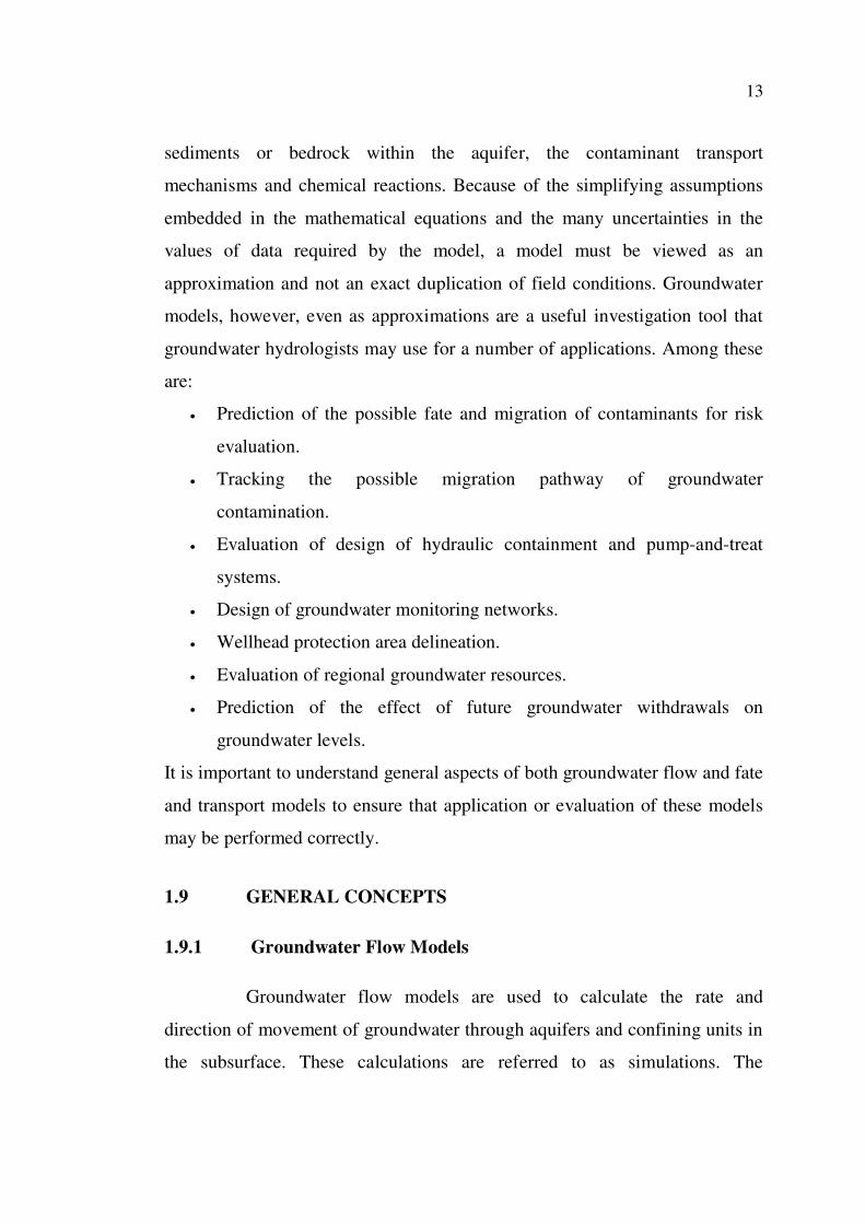
groundwater hydrologists may use for a number of applications. Among these

are:

Prediction of the possible fate and migration of contaminants for risk

evaluation.

Tracking the possible migration pathway of groundwater

contamination.

Evaluation of design of hydraulic containment and pump-and-treat

systems.

Design of groundwater monitoring networks.

Wellhead protection area delineation.

Evaluation of regional groundwater resources.

Prediction of the effect of future groundwater withdrawals on

groundwater levels.

It is important to understand general aspects of both groundwater flow and fate

and transport models to ensure that application or evaluation of these models

may be performed correctly.

1.9 GENERAL CONCEPTS

1.9.1 Groundwater Flow Models

Groundwater flow models are used to calculate the rate and

direction of movement of groundwater through aquifers and confining units in

the subsurface. These calculations are referred to as simulations. The

14

simulation of groundwater flow requires a thorough understanding of the

hydrogeologic characteristics of the site. The hydrogeologic investigation

should include a complete characterization of the following:

Subsurface extent and thickness of aquifers and confining units

(hydrogeologic framework).

Hydrologic boundaries (also referred to as boundary conditions), which

control the rate and direction of movement of groundwater.

Hydraulic properties of the aquifers and confining units.

A description of the horizontal and vertical distribution of hydraulic

head throughout the modeled area for beginning (initial conditions),

equilibrium (steady-state conditions) and transitional conditions when

hydraulic head may vary with time (transient conditions).

Distribution and magnitude of groundwater recharge, pumping or

injection of groundwater, leakage to or from surface-water bodies, etc.

(sources or sinks, also referred to as stresses).

These stresses may be constant (unvarying with time) or may change with

time (transient). The outputs from the model simulations are the hydraulic

heads and groundwater flow rates which are in equilibrium with the

hydrogeologic conditions (hydrogeologic framework, hydrologic boundaries,

initial and transient conditions, hydraulic properties, and sources or sinks)

defined for the modeled area.

Figure 1.4 shows the simulated flow field for a hypothetical site at

which pumping from a well creates changes in the groundwater flow field.

Through the process of model calibration and verification, which is discussed

in later sections of this report, the values of the different hydrogeologic

conditions are varied to reduce any disparity between the model simulations

and field data, and to improve the accuracy of the model. The model can also

be used to simulate possible future changes to hydraulic head or groundwater

15

flow rates as a result of future changes in stresses on the aquifer system

(Predictive simulations are discussed in later sections of this report).

Figure 1.4 Simulated Groundwater Flow Vectors and Hydraulic Head

1.9.2 Fate and Transport Models

Fate and transport models simulate the movement and chemical

alteration of contaminants as they move with groundwater through the

subsurface. Fate and transport models require the development of a calibrated

groundwater flow model or, at a minimum, an accurate determination of the

velocity and direction of groundwater flow, which has been based on field

data. The model simulates the following processes:

Movement of contaminants by advection and diffusion,

Spread and dilution of contaminants by dispersion,

Removal or release of contaminants by sorption or desorption of

contaminants onto or from subsurface sediment or rock, or

Chemical alteration of the contaminant by chemical reactions which

may be controlled by biological processes or physical chemical

reactions.

In addition to a thorough hydrogeological investigation, the simulation of fate

and transport processes requires a complete characterization of the following:

Horizontal and vertical distribution of average linear groundwater velocity

(direction and magnitude) determined by a calibrated groundwater flow model

16

or through accurate determination of direction and rate of groundwater flow

from field data.

Boundary conditions for the solute.

Initial distribution of solute (initial conditions).

Location, history and mass loading rate of chemical sources or sinks.

Effective porosity.

Soil bulk density.

Fraction of organic carbon in soils.

Octanol-water partition coefficient for chemical of concern.

Density of fluid.

Viscosity of fluid.

Longitudinal and transverse dispersivity.

Diffusion coefficient.

Chemical decay rate or degradation constant.

Equations describing chemical transformation processes, if applicable.

Initial distribution of electron acceptors, if applicable.

The outputs from the model simulations are the contaminant concentrations,

which are in equilibrium with the groundwater flow system, and the

geochemical conditions (described above) defined for the modeled area.

Figure 1.5 shows the simulated migration of a contaminant at a hypothetical

site.

Figure 1.5 Simulated Contaminant Plume Migration

17

As with groundwater flow models, fate and transport models should

be calibrated and verified by adjusting values of the different hydrogeologic or

geochemical conditions to reduce any disparity between the model simulations

and field data. This process may result in a re-evaluation of the model used for

simulating groundwater flow if the adjustment of values of geochemical data

does not result in an acceptable model simulation. Predictive simulations may

be made with a fate and transport model to predict the expected concentrations

of contaminants in groundwater as a result of implementation of a remedial

action. The simulated containment of a contaminant plume is shown in Figure

1.5. Monitoring of hydraulic heads and groundwater chemistry will be

required to support predictive simulations.

1.10 TYPES OF MODELS

The equations that describe the groundwater flow and fate and

transport processes may be solved using different types of models. Some

models may be exact solutions to equations that describe very simple flow or

transport conditions (analytical model) and others may be approximations of

equations that describe very complex conditions (numerical model). Each

model may also simulate one or more of the processes that govern

groundwater flow or contaminant migration rather than all of the flow and

transport processes. As an example, particle-tracking models, such as

MODPATH, simulate the advective transport of contaminants but do not

account for other fate and transport processes. In selecting a model for use at a

site, it is necessary to determine whether the model equations account for the

key processes occurring at the site. Each model, whether it is a simple

analytical model or a complex numerical model, may have applicability and

usefulness in hydrogeological and remedial investigations.

18

1.10.1 Analytical Models

Analytical models are an exact solution of a specific, often greatly

simplified, groundwater flow or transport equation. The equation is a

simplification of more complex three-dimensional groundwater flow or solute

transport equations. Prior to the development and widespread use of

computers, there was a need to simplify the three-dimensional equations

because it was not possible to easily solve these equations. Specifically, these

simplifications resulted in reducing the groundwater flow to one dimension

and the solute transport equation to one or two dimensions. This resulted in

changes to the model equations that include one-dimensional uniform

groundwater flow, simple uniform aquifer geometry, homogeneous and

isotropic aquifers, uniform hydraulic and chemical reaction properties, and

simple flow or chemical reaction boundaries. Analytical models are typically

steady-state and one-dimensional, although selected groundwater flow models

are two dimensional (e.g. analytical element models), and some contaminant

transport models assume one-dimensional groundwater flow conditions and

one-, two- or three dimensional transport conditions. An example of output

from a one-dimensional fate and transport analytical model (Domenico and

Robbins, 1985) is shown in Figure 1.6

Because of the simplifications inherent with analytical models, it is

not possible to account for field conditions that change with time or space.

This includes variations in groundwater flow rate or direction, variations in

hydraulic or chemical reaction properties, changing hydraulic stresses, or

complex hydrogeologic or chemical boundary conditions. Analytical models

are best used for:

Initial site assessments where a high degree of accuracy is not needed,

Designing data collection plans prior to beginning field activities,

An independent check of numerical model simulation results, or

19

Sites where field conditions support the simplifying assumptions

embedded in the analytical models.

Figure 1.6 Results from One-Dimensional Fate and Transport Model

1.10.2 Numerical Models

Numerical models are capable of solving the more complex

equations that describe groundwater flow and solute transport. These equations

generally describe multi-dimensional groundwater flow, solute transport and

chemical reactions, although there are one-dimensional numerical models.

Numerical models use approximations (e.g. finite differences, or finite

elements) to solve the differential equations describing groundwater flow or

solute transport. The approximations require that the model domain and time

be discretized. In this discretization process, the model domain is represented

by a network of grid cells or elements, and the time of the simulation is

represented by time steps. A simple example of discretization is presented in

Figure 1.7. The curve represents the continuous variation of a parameter across

the model space or time domain. The bars represent a discrete step-wise

approximation of the curve. The accuracy of numerical models depends upon

the accuracy of the model input data, the size of the space and time

20

discretization (the greater the size of the discretization steps, the greater the

possible error), and the numerical method used to solve the model equations.

Figure 1.7 Example of Discretization Process

Unlike analytical models, numerical models have the capability of

representing a complex multi-layered hydrogeologic framework. This is

accomplished by dividing the framework into discrete cells or elements. An

example of representing a multi-layered aquifer system in a numerical model

is shown in Figure 1.8. In addition to complex three-dimensional groundwater

flow and solute transport problems, numerical models may be used to simulate

very simple flow and transport conditions, which may just as easily be

simulated using an analytical model. However, numerical models are generally

used to simulate problems which cannot be accurately described using

analytical models.

21

Figure 1.8 Example of Discretization of Complex Hydrogeological

Conditions by a Numerical Model

1.11 COMPUTER BASED MODELS

There are several types of computer based models for modeling the

groundwater flow and contaminant transport. Some of them are listed below.

3DFEMFAT: It is a 3-D finite-element model of flow and transport

through saturated-unsaturated media. It is applied for infiltration, wellhead

protection, agriculture pesticides, sanitary landfill, radionuclide disposal sites,

hazardous waste disposal sites, density-induced flow and transport, saltwater

intrusion. It can do simulations of flow only, transport only, combined

22

sequential flow and transport, or coupled density-dependent flow and

transport.

AQUA3D: It is a 3-D groundwater flow and contaminant transport

model. It solves transient groundwater flow within homogeneous and

anisotropic flow conditions. It also solves transient transport of contaminants

and heat with convection, decay, adsorption and velocity-dependent

dispersion.

AT123D: It is a analytical groundwater transport model for long-

term pollutant fate and migration. It computes the spatial-temporal

concentration distribution of wastes in the aquifer system and predicts the

transient spread of a contaminant plume through a groundwater aquifer on a

monthly basis for up to 99 years of simulation time.

BIOF&T 2-D/3-D: It is for biodegradation, flow and transport in the

saturated / unsaturated zones. It allows real world modeling not adsorption.

Desorption, and microbial process based on oxygen -limited, anaerobic, first-

order, or Monod-type biodegradation kinetics as well as anaerobic or first-

order sequential degradation involving multiple daughter species.

Chemflo: It simulates movement of water and chemical in

unsaturated soils. The equations are solved numerically for one dimensional

flow and transport using finite differences.

Chem Flux: It is a finite element mass transport model. It predicts

the movement of contaminant plumes through the processes of advection,

diffusion, adsorption and decay. It provides an elegant and simple user

interface.

23

FEFLOW: Finite element subsurface flow system. It simulates 3D

and 2D fluid density-coupled flow, contaminant mass (salinity) and heat

transport in the subsurface. It is capable of computing: a). groundwater

systems with and without free surfaces (phreatic aquifers, perched water

tables, moving meshes, b). problems in saturated-unsaturated zones, c). both

salinity-dependent and transport phenomena (thermohaline flows), d).

complex geometric and parametric situations.

FLONET/TRANS: It is a 2-D cross sectional groundwater flow and

contaminant transport model. It uses the dual formation of hydraulic potentials

and streamlines to solve the saturated groundwater flow equation and create

accurate flownet diagrams for any two-dimensional, saturated groundwater

flow system. It also simulates advective-dispersive contaminant transport

problems with spatially-variable retardation and multiple source terms.

FLOWPATH: 2-D groundwater flow, remediation, and wellhead

protection model. It is for groundwater flow, remediation, and wellhead

protection. It is a comprehensive modeling environment transport in

unconfined, confined and leaky aquifers with heterogeneous properties,

multiple pumping wells and complex boundary conditions. Typical application

includes a). Determining remediation well capture zones, b). delineating

wellhead protection areas, c). designing and optimizing pumping well

locations for dewatering projects, d). determining contaminant fate and

exposure pathways for risk assessment.

GFLOW: It is analytic element model with conjunctive surface

water and groundwater flow and a modflow model extract feature. It is an

efficient stepwise groundwater flow modeling system. It models steady-state

flow in a single heterogeneous aquifer using the Dupuit-Forchheimer

assumption.

24

GMS: Groundwater Modeling Environment for MODFLOW,

MODPATH, MT3D, RT3D, FEMWATER, SEAM3D, SEEP2D, PEST,

UTCHEM, and UCODE. It is a sophisticated and comprehensive groundwater

modeling software. It provides tools for every phase of a groundwater,

simulation including site characterization, model development, calibration,

post-processing, and visualization.

Groundwater Vistas (GV): It is a sophisticated windows graphical

user interface for 3-D groundwater flow and transport modeling. It couples a

model design system with comprehensive graphical analysis tools. GV is a

model-independent graphical design system for MODFLOW, MODPATH,

MT3DMS, RT3D, PARH3D, PEST, UCODE, SEWWAT, MODFLOWT-

SURFACT, MODFLOW2000.

HST3D: It is a 3-D heat and solute transport model and a powerful

user-friendly interface for HST3D integrated within the Argus Open

Numerical Environments (Argus ONE) modeling environment. HST3D allows

the user to enter all spatial data, graphically run HST3D, and visualize the

results.

MicroFEM: Finite-element program for multiple-aquifer steady-

state and transient groundwater flow modeling. It is a new program, based on

the DOS package Micro-Fem. It demonstrates the whole process of ground-

water modeling, from the generation of a finite-element grid through the stages

of preprocessing, calculation, post processing, graphical interpretation and

plotting. Confined, semi-confined, phreatic, stratified and leaky multi-aquifer

systems can be simulated with a maximum of 20 aquifers.

MOC: This is a 2-D model for solute transport and dispersion in

groundwater. It is applicable for one-or two-dimensional problems involving

25

steady-state or transient flow. MOC computes changes in concentration over

time caused by the processes of convective transport, hydrodynamic

dispersion, and mixing (or dilution) from fluid sources. MOC is based on a

rectangular, block centered, finite-difference grid. It can also be used for

heterogeneous and/or anisotropic aquifer.

MOCDENSE: Two-constituent solute transport model for

groundwater having variable density. It simulates the flow in a cross-sectional

plane rather than in an aerial plane. Because the problem of interest involves

variable density, the model solves for fluid pressure rather than hydraulic head

in the flow equation. The solution to the flow equation is obtained using finite-

difference method. Solute transport is simulated with the method of

characteristics. Density is considered to be a function of the concentration of

the one of the constituents.

MODFLOW: This is a three-dimensional ground water flow model.

MODFLOW has become the worldwide standard ground-water flow model.

MODFLOW is used to simulate systems for water supply, containment

remediation and mine dewatering. The modular structure of MODFLOW

consists of a main Program and a series of highly-independent subroutines

called modules. The modules are grouped in packages. Each package deals

with a specific feature of the hydrologic system which is to be simulated such

as flow from rivers or flow into drains or with a specific method of solving

linear equations which describe the flow system.

MODFLOW SURFACT: It is a new flow and transport model and

it is based on the USGS MODFLOW code, the most widely-used ground-

water flow code in the world. MODFLOW has certain limitations in

simulating complex filed problems. Additional computational modules have

26

been incorporated to enhance the simulation capabilities and robustness. It is a

seamless integration flow and transport modules.

MODFLOWT: This is an enhanced version of MODFLOW for

simulating 3-D contaminant transport This includes packages to simulate

advective-dispersive contaminant transport. It performs groundwater

simulations utilizing transient transport with steady-state flow, transient flow,

or successive periods of steady-state flow.

MODFLOWwin32: (MODFLOW for Windows) The model has all

the features of other MODFLOW versions and the new packages which

include stream routing, aquifer compaction, horizontal flow barrier, BCF2, and

BCF3 packages and the new PCG2 solver. In addition, it will create files for

use with MODPATH (particle-tracking model for MODFLOW) and MT3D

(solute transport model).

MODPATH: It is a 3-D particle tracking post processing package

for MODFLOW, the USGS 3-D finite-difference ground-water flow model. It

is a widely used particle tracking program.

MOFAT: It is multiphase (water, oil, gas) flow and multi

component transport model. Simulate multiphase flow and transport of up to

five non-inert chemical species in MOFAT. Simulate dynamic or passive gas

as a full three-phase flow problem. Model water flow only, oil-water flow, or

water-oil-gas flow in variably-saturated porous media.

MS-VMS: It is a comprehensive MODFLOW-based visual

modeling system for ground-water flow and contaminate transport. It over

comes the limitations of MODFLOW.

27

MT3D: It is a comprehensive three-dimensional numerical model

for simulating solute transport in complex hydrogeologic settings. MT3D has a

modular design that permits simulation of transport processes independently or

jointly. MT3D is capable of modeling advection in complex steady-state and

transient flow fields, anisotropic dispersion, first-order decay and production

reactions, and linear and nonlinear sorption. MT3D is linked with groundwater

flow simulator MODFLOW and it is designed specifically to handle

advectively-dominated transport problems without the need to consider refined

methods specifically for solute transport.

PEST: It is a nonlinear parameter estimation and optimization

package. It can be used to estimate parameters for just about any existing

model whether or not you have the model’s source code.

PESTAN: It is a pesticide transport model. It is a USEPA program

for evaluating the transport of organic solutes through the vadose zone to

groundwater. Input data includes water solubility, infiltration rate, bulk

density, sorption constant, degradation rates, saturated water content, saturated

hydraulic conductivity and dispersion coefficient.

POLLUTE: It is a finite layer contaminant migration model for

landfill design. It can be used for fast, accurate and comprehensive

contaminant migration analysis. Landfill designs that can be considered range

from simple systems on a natural aquitard to composite liners with multiple

barriers and multiple aquifers.

PRINCE: It is a well known software package of ten analytical

groundwater models originally developed as part of an EPA 208 study. There

are seven one, two and three-dimensional mass transport models and three

two-dimensional flow models in PRINCE. These groundwater models have

28

been rewritten from the original mainframe FORTRAN codes. Two popular

analytical models have been added to the original collection, and the ability to

import digitized or AutoCAD-produced DXF site map files has been added.

PRZM3: It links two models, PRZM and VADOFT to predict

pesticide transport and transformation down through the crop root and vadose

(unsaturated) zone to the water table. PRZM3 incorporates soil temperature

simulation, volatilization and vapour phase transport in soils, irrigation

simulation, and microbial transformation. PRZM is a one-dimensional finite-

difference model which uses a method of characteristics (MOC) algorithm to

estimate numerical dispersion. VADOFT is a one-dimensional finite-element

code that solves Richards’ equation for flow in the unsaturated zone. The user

may make use of constituting relationships between pressure, water content,

and hydraulic conductivity to solve the flow equation. PRZM3 is capable of

simulating multiple pesticides or parent-daughter relationships. PRZM3 is also

capable of estimating probabilities of concentrations or fluxes in or from

various media for the purpose of performing exposure assessments.

RBCA Tier 2 Analyzer: It is a two-dimensional groundwater model

with a comprehensive selection of contaminant transport simulation

capabilities including single or multiple species sequential decay reactions

such as reductive dechlorination of PCE instantaneous or kinetic-limited

BTEX biodegradation with single or multiple electron acceptors and

equilibrium or non-equilibrium sorption.

SEAWAT: It is a three-dimensional variable-density ground-water

flow model for porous media. The source code was developed by combining

MODFLOW and MT3DMS into a single program that solves the coupled flow

and solute-transport equations. The SEAWAT code follows a modular

structure, and thus, new capabilities can be added with only minor

29

modifications to the main program. SEAWAT reads and writes standard

MODFLOW and MT3DMS data sets, although some extra input may be

required for some SEAWAT simulations. This means that many of the existing

pre and post processors can be used to create input data sets and analyze

simulation results.

SESOIL: It is a seasonal compartment model which simulates long-

term pollutant fate and migration in the unsaturated soil zone. SESOIL

describes the following components of a user-specified soil column which

extends from the ground surface to the ground-water table. a). Hydologic cycle

of the unsaturated soil zone, b). pollutant concentrations and masses in water,

soil, and air phases, c). pollutant migration to groundwater, d). pollutant

volatilization at the ground surface, e). pollutant transport in wash load due to

surface runoff and erosion at the ground surface. SESOIL estimates all of the

above components on a monthly basis for up to 999 years of simulation time.

It can be used to estimate the average concentrations in groundwater. The soil

column may be composed of up to four layers, each layer having different soil

properties which affect the pollutant fate. In addition, each soil layer may be

subdivided into a maximum of 10 sub layers in order to provide enhanced

resolution of pollutant fate and migration in the soil column. The following

pollutant fate processes are accounted for : volatilization, adsorption, cation

exchange, biodegradation, hydrolysis and complexation.

SLAEM / MLAEM: It is based on analytic element method. The

computer program is intended for modeling regional groundwater flow in

systems of confined, unconfined, and leaky aquifers. SLAEM is single layer

analytic model and MLAEM is a multi layer analytic model. All programs run

under MS Windows 95, 98 and NT. The programs are native windows

applications and are accessed via a modern and flexible Graphical User

Interface (GUI), as well as via a command-line interface. The latter capability

30

makes it easy to drive the program from other programs such as Arc-View,

ARC/INFO and PEST. The programs read DXF-files and produce BNA files

that may be read by other programs such as SURFER.

SOLUTRANS: It is a 32-bit Windows program for modeling three-

dimensional solute transport based on the solutions presented by Leij et al. for

both equilibrium and non-equilibrium transport. The interface and input

requirements are so simple that it only takes a few minutes to develop models

and build insight and complex solute transport problems. With SOLUTRANS

we can, in a matter of minutes, model solute transport from a variety of source

configurations and build important insights about key processes. It offers a

quick and simple alternative to complex, time-consuming 3-D numerical flow

and transport models.

SUTRA: It is a 2D groundwater saturated-unsaturated transport

model, a complete saltwater intrusion and energy transport model. SUTRA

simulates fluid movement and transport of either energy or dissolved

substances in a subsurface environment. SUTRA employs a two-dimensional

hybrid finite-element and integrated finite-difference method to approximate

the governing equations that describe the two interdependent processes that are

simulated: (i) fluid density-dependent saturated or unsaturated groundwater

flow and either (iia) transport of a solute in the groundwater, in which the

solute may be subjected to equilibrium adsorption on the porous matrix and

both first-order and zero-order production or decay, or (iib) transport of

thermal energy in the groundwater and solid matrix of he aquifer.

SVFlux 2D: It represents the next level in seepage analysis

software. Designed to be simple and effective, the software offers features

designed to allow the user to focus on seepage solutions, not convergence

problems or different mesh creation.

31

SWIFT: It is fully-transient, three-dimensional model to simulate

groundwater flow, heat (energy), brine and radionuclide transport in porous

and fractured geologic media. In addition to transient analysis, SWIFT offers a

steady-state option for coupled flow and brine. The equations are solved using

central or backward spatial and time weighting approximations by the finite-

difference methods. In addition to Cartesian, cylindrical grids may be used.

Contaminant transport includes advection, dispersion, sorption and decay,

including chains of constituents.

SWIMv1: It is software package (version1) for simulating water

infiltration and movement in soils. It consists of a menu-driven suite of three

programs that allow the user to simulate soil water balances using numerical

solutions of the basic soil water flow equations. As in real world, SWIMv1

allows addition of water to the system as precipitation and removal by runoff,

drainage, evaporation from the soil surface and transpiration by vegetation.

SWIMv1 helps to understand the soil water balance so they can assess possible

effects of such practices as tree clearing, strip mining and irrigation

manganese.

TWODAN: It is a popular and versatile analytic groundwater flow

model for Windows. TWODAN has suite of advanced analytic modeling

features hat allow you to model everything from a single well in a uniform

flow filed to complex remediation schemes with numerous wells, barriers,

surface waters, and heterogeneities. TWODAN has many capabilities:

heterogeneities, impermeable barriers, resistant barriers, and transient

solutions. It can be used for modeling remedial design alternatives, wellhead

capture zones, and regional aquifer flow.

VAM2D: It is a two dimensional finite-element groundwater model

that simulates transient or steady-state groundwater flow and contaminant

32

transport in porous media. VAM2D analyzes unconfined flow problems using

a rigorous saturated-unsaturated modeling approach using efficient numerical

techniques. Accurate mass balance is maintained in VAM2D even when

simulating highly nonlinear soil moisture relations. Hysteresis effects in the

water retention curve can also be simulated. A wide range of boundary

conditions can be treated in VAM2D including seepage faces, water-table

conditions, recharge, infiltration, evapotranspirtaion, and pumping and

injection wells. The contaminant transport option can account for advection,

hydrodynamic dispersion, equilibrium sorption, and first-order degradation.

Transport of a single species or multiple parent-daughter components of a

decay chain can be simulated. This model can perform simulations using an

areal plane, cross section, or axisymmentric configuration.

Visual Groundwater: It is a 3-D visualization software package

which can be used to deliver high-quality, three-dimensional presentations of

subsurface characterization data and groundwater modeling results. Visual

Groundwater combines state-of-the-art graphical tools for 3-D visualization

and animation with a data management system specifically designed for

borehole investigation data. This model also comes with a data conversion

utility to create 3-D data files using X,Y,Z data, and girded data sets. Three-

dimensional images of complex site characterization data and modeling results

can be easily created.

VISUAL HELP: It is an advanced hydrological modeling

environment available for designing landfills, predicting leachate mounding

and evaluating potential leachate contamination. Visual HELP combines the

latest version of the HELP model with an easy-to user interface and powerful

graphical features for designing the model and evaluating the modeling results.

33

Visual MODFLOW: It provides professional 3D groundwater flow

and contaminant transport modeling using MODFLOW-2000, MODPATH,

MT3DMS and RT3D. It allows to: a). graphically design the model grid,

properties and boundary conditions, b). visualize the model input parameters

in two or three dimensions, c). run the groundwater flow, pathline and

contaminant transport simulations, d). automatically calibrate the model using

Win PEST or manual methods, e). display and interpret the modeling results in

three-dimensional space using the Visual MODFLOW 3D-Explorer. This

model (version2.8.1) is used in this research and it is explained in detail in

Chapter-3.

VISUAL PEST: It combines the powerful parameter estimation

capabilities of PEST2000 with the graphical processing and display features of

WinPEST. PEST2000 is the latest version of PEST, the pioneer in model-

independent parameter estimation. It has undergone continued development

with addition of many features that have improved its performance and utility

to a level that makes it uniquely applicable in any modeling environment.

VLEACH: It is a one-dimensional finite-difference vadose zone

leaching, model developed by US EPA. It describes the movement of an

organic contaminant within and between three phases: i) as a solute dissolved

in water, (ii) as a gas in the vapour phase, and (iii) as an adsorbed compound

in the solid phase. The leaching is simulated in a number of distinct, user-

defined polygons vertically divided into a series of user-defined cells. At the

end of the simulation, the results from each polygon are used to determine an

area-weighted ground-water impact due to the mobilization and migration of a

sorbed organic contaminant located in the vadose zone on the underlying

groundwater resource.

34

VS2DT: It is a USGS program for flow and solute transport in

variably-saturated, single-phase flow in porous media. A finite-difference

approximation is used in VS2DT to solve the advection-dispersion equation.

Simulated regions include one-dimensional columns, two-dimensional vertical

cross sections, and axially-symmetric, three-dimensional cylinders. The

VS2DT program options include backward or centered approximations for

both space and time derivatives, first-order decay, equilibrium adsorption

(Freundlich or Langmuir) isotherms, and ion exchange. Nonlinear storage

terms are storage terms are linearized by an implicit Newton-Raphson method.

Relative hydraulic conductivity in VS2DT is evaluated at cell boundaries

using full upstream weighting, arithmetic mean or geometric mean.

WHI UnSat Suite: It combines SESOIL, VLEACH, PESTAN,

VS2DT and HELP in a revolutionary graphical environment specifically

designed for simulating one-dimensional groundwater flow and contaminant

transport through he unsaturated zone. All five of these models are compiled

and optimized to run as native Windows applications and are seamlessly

integrated within the WHI UnSat Suite modeling environment. It can be used

for (i) simulate long-term pollutant fate and transport (VOCs, PAHs, pesticides

and heavy metals) in the unsaturated zone under seasonally variable conditions

using SESOIL, (ii) predict vertical migration of volatile hydrocarbons through

the vadose zone using VLEACH, (iii) estimate agricultural pesticide migration

through the unsaturated zone using PESTAN, (iv) simulate groundwater flow

and transport processes through heterogeneous, unsaturated soil using VS2DT,

(v) predict seasonal recharge rates through heterogeneous soil conditions

under variable weather conditions using the HELP model, (vii) generate up to

100 years of statistically reliable climatologically data for virtually any

location in the world using the WHI weather generator.

35

WinTran: It couples the steady-state groundwater flow model from

WinFlow with a contaminant transport model. The transport model has the feel

of an analytic model but is actually an embedded finite-element simulator. The

finite-element transport model is constructed automatically by WinTran but

displays numerical criteria (Peclet and Courant numbers) to allow the user to

avoid numerical or mass balance problems. Contaminant mass may be injected

or extracted using any of the analytic elements including wells, ponds, and

linesinks. In addition, constant concentration elements have been added.

WinTran displays both head concentration contours, and concentration may be

plotted versus time at selected monitoring locations. The transport model

includes the effects of dispersion, linear sorption (retardation), and first-order

decay. WinTran aids in risk assessment calculations by displaying the

concentration over time at receptor or observation locations. WinTran will

display the breakthrough curves after the simulation is finished.

1.12 GROUNDWATER MODEL DEVELOPMENT PROCESS

1.12.1 Hydrogeologic Characterization

Proper characterization of the hydrogeological conditions at a site is

necessary in order to understand the importance of relevant flow or solute-

transport processes. With the increase in the attempted application of natural

attenuation as a remedial action, it is imperative that a thorough site

characterization be completed. This level of characterization requires more

site-specific fieldwork than just an initial assessment, including more

monitoring wells, groundwater samples, and an increase in the number of

laboratory analytes and field parameters. Without proper site characterization,

it is not possible to select an appropriate model or develop a reliably calibrated

model. At a minimum, the following hydrogeological and geochemical

information must be available for this characterization:

36

Regional geologic data depicting subsurface geology.

Topographic data (including surface-water elevations)

Presence of surface-water bodies and measured stream-discharge (base

flow) data

Geologic cross sections drawn from soil borings and well logs.

Well construction diagrams and soil boring logs.

Measured hydraulic-head data.

Estimates of hydraulic conductivity derived from aquifer and/or slug

test data.

Location and estimated flow rate of groundwater sources and sinks.

Identification of chemicals of concern in contaminant plume*.

Vertical and horizontal extent of contaminant plume*.

Location, history, and mass loading or removal rate for contaminant

sources or sinks*.

Direction and rate of contaminant migration*.

Identification of downgradient receptors*.

Organic carbon content of sediments*.

Appropriate geochemical field parameters (e.g. dissolved oxygen, Eh,

pH)*

Appropriate geochemical indicator parameters (e.g. electron acceptors,

and degradation byproducts)*

* Required only by fate and transport models.

These data should be presented in map, table, or graph format in a report

documenting model development.

1.12.2 Model Conceptualization

Model conceptualization is the process in which data describing

field conditions are assembled in a systematic way to describe groundwater

flow and contaminant transport processes at a site. The model

37

conceptualization aids in determining the modeling approach and which model

software to use. Questions to ask in developing a conceptual model include,

but are not limited to:

Are there adequate data to describe the hydrogeological conditions at

the site?

In how many directions is groundwater moving?

Can the groundwater flow or contaminant transport be characterized as

one-, two- or three dimensional?

Is the aquifer system composed of more than one aquifer, and is vertical

flow between aquifers important?

Is there recharge to the aquifer by precipitation or leakage from a river,

drain, lake, or infiltration pond?

Is groundwater leaving the aquifer by seepage to a river or lake, flow to

a drain, or extraction by a well?

Does it appear that the aquifer's hydrogeological characteristics remain

relatively uniform, or do geologic data show considerable variation

over the site?

Have the boundary conditions been defined around the perimeter of the

model domain, and do they have a hydrogeological or geochemical

basis?

Do groundwater-flow or contaminant source conditions remain

constant, or do they change with time?

Are there receptors located downgradient of the contaminant plume?

Are geochemical reactions taking place in onsite groundwater, and are

the processes understood?

Other questions related to site-specific conditions may be asked. This

conceptualization step must be completed and described in the model

documentation report.

38

1.12.3 Model Software Selection

After hydrogeological characterization of the site has been

completed, and the conceptual model developed, computer model software is

selected. The selected model should be capable of simulating conditions

encountered at the site. The following general guidelines should be used in

assessing the appropriateness of a model: Analytical models should be used

where: (i) field data show that groundwater flow or transport processes are

relatively simple, (ii) an initial assessment of hydrogeological conditions or

screening of remedial alternatives is needed. Numerical models should be used

where: (i) field data show that groundwater flow or transport processes are

relatively complex, (ii) groundwater flow directions, hydrogeological or

geochemical conditions, and hydraulic or chemical sources and sinks vary

with space and time. A one-dimensional groundwater flow or transport model

should be used primarily for initial assessments where the degree of aquifer

heterogeneity or anisotropy is not known and for sites where a potential

receptor is immediately downgradient of a contaminant source. Two-

dimensional models should be used for (i) problems which include one or

more groundwater sources/sinks (e.g. pumping or injection wells, drains,

rivers, etc.), (ii) sites where the direction of groundwater flow is obviously in

two dimensions(e.g. radial flow to a well, or single aquifer with relatively

small vertical hydraulic head or contaminant concentration gradients), (iii)

sites at which the aquifer has distinct variations in hydraulic properties, (iv)

contaminant migration problems where the impacts of transverse dispersion

are important and the lateral, or vertical, spread of the contaminant plume must

be approximated. Three-dimensional flow and transport models should

generally be used where the hydrogeologic conditions are well known,

multiple aquifers are present, the vertical movement of groundwater or

contaminants is important. The rationale for selection of the appropriate model

software should be discussed in the model documentation report.

39

1.12.4 Model Calibration

Model calibration consists of changing values of model input

parameters in an attempt to match field conditions within some acceptable

criteria. This requires that field conditions at a site be properly characterized.

Lack of proper site characterization may result in a model that is calibrated to

a set of conditions which are not representative of actual field conditions. The

calibration process typically involves calibrating to steady-state and transient

conditions. With steady-state simulations, there are no observed changes in

hydraulic head or contaminant concentration with time for the field conditions

being modeled. Transient simulations involve the change in hydraulic head or

contaminant concentration with time (e.g. aquifer test, an aquifer stressed by a

well-field, or a migrating contaminant plume). These simulations are needed to

narrow the range of variability in model input data since there are numerous

choices of model input data values which may result in similar steady-state

simulations. Models may be calibrated without simulating steady-state flow

conditions. At a minimum, model calibration should include comparisons

between model-simulated conditions and field conditions for the following

data: hydraulic head data, groundwater-flow direction, hydraulic-head

gradient, water mass balance, contaminant concentrations (if appropriate),

contaminant migration rates (if appropriate), migration directions (if

appropriate), and degradation rates (if appropriate).

These comparisons should be presented in maps, tables, or graphs.

A simple graphical comparison between measured and computed heads is

shown in Figure 1.9. In this example, the closer the heads fall on the straight

line, the better the “goodness-of-fit”. Each modeler and model reviewer will

need to use their professional judgment in evaluating the calibration results.

There are no universally accepted “goodness-of-fit” criteria that apply in all

cases. However, it is important that the modeler make every attempt to

40

minimize the difference between model simulations and measured field

conditions. Typically, the difference between simulated and actual field

conditions (residual) should be less than 10 percent of the variability in the

field data across the model domain. A plot showing residuals at monitoring

wells (calibration targets) is shown in Figure 1.10. A plot in this format is

useful to show the “goodness-of-fit” at individual wells.

The modeler should also avoid the temptation of adjusting model

input data on a scale which is smaller than the distribution of field data. This

process, referred to as "over calibration", results in a model that appears to be

calibrated but has been based on a dataset that is not supported by field data.

For initial assessments, it is possible to obtain useful results from models that

are not calibrated. The application of uncalibrated models can be very useful

in guiding data collection activities for hydrogeological investigations or as a

screening tool in evaluating the relative effectiveness of remedial action

alternatives.

Figure 1.9 Comparison between Measured and Computed Hydraulic

Heads

41

Figure 1.10 Residuals from Comparison of Measured and Computed

Heads at Calibration Targets

1.12.5 History Matching

A calibrated model uses selected values of hydrogeologic

parameters, sources and sinks and boundary conditions to match field

conditions for selected calibration time periods (either steady-state or

transient). However, the choice of the parameter values and boundary

conditions used in the calibrated model is not unique, and other combinations

of parameter values and boundary conditions may give very similar model

results. History matching uses the calibrated model to reproduce a set of

historic field conditions. This process has been referred to by others as “model

verification”.

The most common history matching scenario consists of

reproducing an observed change in the hydraulic head or solute concentrations

over a different time period, typically one that follows the calibration time

period (Figure 1.11). The best scenarios for model verification are ones that

use the calibrated model to simulate the aquifer under stressed conditions. The

process of model verification may result in the need for further calibration

42

refinement of the model. After the model has successfully reproduced

measured changes in field conditions for both the calibration and history

matching time periods, it is ready for predictive simulations.

Figure 1.11 Comparison between Computed and Observed Heads with

Time

1.12.6 Sensitivity Analysis

A sensitivity analysis is the process of varying model input

parameters over a reasonable range (range of uncertainty in values of model

parameters) and observing the relative change in model response (Figure

1.12). Typically, the observed changes in hydraulic head, flow rate or

contaminant transport are noted. The purpose of the sensitivity analysis is to

demonstrate the sensitivity of the model simulations to uncertainty in values of

model input data. The sensitivity of one model parameter relative to other

parameters is also demonstrated. Sensitivity analyses are also beneficial in

determining the direction of future data collection activities. Data for which

the model is relatively sensitive would require future characterization, as

opposed to data for which the model is relatively insensitive. Model-

insensitive data would not require further field characterization.

43

Figure 1.12 Simulated Change in Hydraulic Head Resulting from Change

in Parameter Value

1.12.7 Predictive Simulations or Evaluation of Remediation

Alternatives

A model may be used to predict some future groundwater flow or

contaminant transport condition. The model may also be used to evaluate

different remediation alternatives, such as hydraulic containment, pump-and-

treat or natural attenuation, and to assist with risk evaluation. In order to

perform these tasks, the model, whether it is a groundwater flow or solute

transport model, must be reasonably accurate, as demonstrated during the

model calibration process. However, because even a well-calibrated model is

based on insufficient data or oversimplifications, there are errors and

uncertainties in a groundwater-flow analysis or solute transport analysis that

make any model prediction no better than an approximation. For this reason,

all model predictions should be expressed as a range of possible outcomes

which reflect the uncertainty in model parameter values. The range of

uncertainty should be similar to that used for the sensitivity analysis. The

following examples demonstrate, in a limited manner, how model predictions

may be presented to illustrate the range of possible outcomes resulting in

model input data uncertainty. Figure 1.13 shows the range in computed head at

44

calibration targets at a particular point in time resulting from varying a model

parameter over its range of uncertainty. If the purpose of the predictive

simulations is to determine the future hydraulic head distribution in an aquifer,

the upper and lower estimate of head should be presented so that appropriate

decisions may be made.

Figure 1.13 Simulated Uncertainty in Hydraulic Heads at Calibration

Targets

In the following example (Figure 1.14), hydraulic heads are

predicted for a future time interval in response to changing stresses on the

aquifer system. The predicted results using the calibrated flow model are

presented as the black line. The red and blue lines show the hydraulic heads

predicted using slightly different model input parameters which result in

values of hydraulic head which are five percent higher and lower than the

heads predicted using the calibrated model. Again, the range in predicted

heads should be presented so that appropriate, or conservative, decisions may

be made regarding the groundwater resource.

45

Figure 1.14 Predicted Range in Hydraulic Heads

Figure 1.15 shows an example of delineating a wellhead protection

area (WHPA) for a public water-supply. These WHPAs were simulated using

the range of hydraulic conductivity values reported from an aquifer test at a

municipal well. The WHPA delineated using the low hydraulic conductivity

value (shown in brown) is wider than and not as long as the WHPA delineated

using the high value of hydraulic conductivity (shown in gold). In order to be

protective of the public water supply, it's important that the delineated WHPA

is conservatively estimated. In this example, the final recommended WHPA is

a composite of the two previously simulated WHPAs.

Figure 1.15 Simulated Wellhead Protection Areas Using Range of

Hydraulic Conductivities

46

This final example (Figure 1.16) shows the simulated contaminant

concentrations downgradient from a source area. The purpose of the

simulation was to estimate the contaminant concentration at the point of

compliance, approximately 1000 feet downgradient from the source area. The

difference between the two simulations shown in the figure is the value of

organic carbon fraction used in each simulation. Increasing the organic carbon

concentration increases the degree of attenuation of the contaminant plume.

Since the organic carbon content of sediments is very seldom known with a

high degree of certainty, and a single value is typically used in fate and

transport models, it is best to present the simulation results as a range of

concentrations which might result. This can be said for any of the model input

parameters used in fate and transport models.

Figure 1.16 Simulated Contaminant Concentrations

1.13 GROUNDWATER MODELS AND PERFORMANCE

MONITORING

Groundwater models are used to predict the migration pathway and

concentrations of contaminants in groundwater. The accuracy of model

predictions depends upon successful calibration and verification of the model

in determining groundwater flow directions, transport of contaminants and

chemical reactions, and the applicability of the groundwater flow and solute

47

transport equations to the problem being simulated. Errors in the predictive

model, even though small, can result in gross errors in solutions projected

forward in time. Among other things, performance monitoring is required to

compare future field conditions with model predictions to assess model error.

1.13.1 Predictive Simulations

Predictive simulations may be used to estimate the hydraulic

response of an aquifer, the possible migration pathway of a contaminant, the

contaminant mass removal rate from an aquifer, or the concentration of a

contaminant at a point of compliance at some future point in time. The

predictive simulations must be viewed as estimates, not certainties, to aid the

decision-making process. As an example, the design of a groundwater

remediation system may be based on predictive model simulations. A model

may be used to predict the pumping rate needed to capture a contaminant

plume and to estimate the contaminant concentration of the extracted

groundwater. Monitoring of hydraulic heads and contamination concentrations

must be used to verify hydraulic containment and remediation of the

contaminant plume. Predictive simulations are based on the conceptual model

developed for the site, the values of hydrogeological or geochemical

parameters used in the model, and on the equations solved by the model

software. Errors in values of model parameters, or differences between field

conditions and the conceptual model or model equations will result in errors in

predictive simulations. Models are calibrated by adjusting values of model

parameters until the model response closely reproduces field conditions within

some acceptable criteria in an attempt to minimize model error. However, the

time period over which a model is calibrated is typically very small, especially

when compared to the length of time used for predictive simulations.

Relatively small errors observed during the time period over which the model

calibration or history matching was performed may be greatly magnified

48

during predictive simulations because of the greater time period length

typically used in predictive simulations. The growth in errors resulting from

projecting model simulation into the future need to be evaluated by monitoring

field conditions over the time period of the predictive simulation or until

appropriate cleanup criteria have been achieved. There is always some degree

of uncertainty in predictive models. Predictive models should be conservative.

That is, given the uncertainty in model input parameters and the corresponding

uncertainty in predictive model simulations, model input values should be

selected which result in a “worst-case” simulation. Site-specific data may be

used to support a more reasonable worst-case scenario. Or stated another way,

site-specific data should be collected to limit the range of uncertainty in

predictive models. Further re-calibration of the model to minimize the

difference between model simulations and performance monitoring data may

not be warranted.

Figure 1.17 Example of Growth of Model Error in Predictive Simulation

1.13.2 Performance Monitoring

As previously stated, groundwater model simulations are an

approximation of the actual system behavior and monitoring of field

conditions are needed to evaluate error in model predictions. Performance

49

monitoring is required as a means of physically measuring the actual behavior

of the hydrogeologic system and demonstrating compliance with

environmental statutes. Groundwater model simulations are estimates and may

not be substituted in place of measurement of field data. Examples of

applications of contaminant transport and groundwater modeling requiring

performance monitoring would include, but not be limited to the following:

Hydraulic containment systems for which certain geochemical and

hydraulic head criteria, which measure the success of the remedial action,

have been specified in a remedial action plan.

Groundwater/surface-water interface (GSI) mixing zones for which the

chemistry of the contaminant plume discharging to a surface-water body

must meet appropriate criteria.

Natural attenuation remedies in which a contaminant transport model

predicts that site specific contaminants will reach regulatory limits prior to

reaching a specified point.

The degree of performance monitoring required at a site depends on

the conditions or actions which have been simulated and the associated level

of risk to the downgradient receptors, if applicable. Hydraulic-head monitoring

points should be at well distributed locations to demonstrate the desired

hydraulic response. Monitoring of groundwater chemistry would be needed at

locations downgradient of, or lateral to, the hydraulic containment system,

with less frequent chemical monitoring at locations within the capture zone of

the system. Sites at which contaminant biodegradation has been simulated

would require extensive monitoring of appropriate chemical parameters and

less frequent monitoring of hydraulic heads. Chemical monitoring would be

required at a sufficient number of locations to evaluate the migration or mass

removal of contaminants and groundwater quality at the designated points of

compliance. The performance monitoring will be based ultimately on actual

laboratory analytical data and the chemical criteria established for the site.