Chap. II, Sec. 1.2: Inspiral of (quasi)elliptic binaries

We now repeat (pretty much) the entire previous subsection in themore general case of a (quasi)elliptic binary.

The first thing to do is thus to establish a convenientparametrization of the orbit. The orbit is still confined to a plane,by conservation of angular momentum, but now its timedependence it rather more involved. We won’t give the (somewhatcomplicated) derivations here, but will simply note that theseparation r is given as a function of the true anomaly ψ by

r =a(1− e2)

1 + e cosψ,

and

ψ =

√ma(1− e2)

r2=

√m

a3(1 + e cosψ)2

(1− e2)3/2,

by Kepler’s second law (i.e., conservation of angular momentum).

GW luminosityWe begin by noting that it is most convenient to write the(traceful!) mass quadrupole moment in matrix form (withcoordinates in the plane of the orbit) as

Mkl.

= µr2[

cos2 ψ sinψ cosψsinψ cosψ sin2 ψ

],

and use the expression for r in terms of ψ. We then computederivatives using the expression for ψ. See Sec. 4.1 in Maggiore for the details.

The resulting expression for the “instantaneous luminosity” is thus

Linst(ψ) =8

15

µ2m3

a5(1− e2)5(1+e cosψ)4[12(1+e cosψ)2+e2 sin2 ψ].

Of course, this “instantaneous luminosity” has no meaning, assuch (and is possibly even misleading terminology). We really want to average thisover several wavelengths of the emitted radiation (and since themotion is [quasi]periodic, an average over a period suffices).

GW luminosity (cont.)

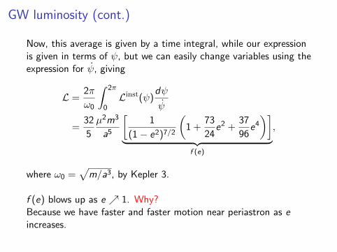
Now, this average is given by a time integral, while our expressionis given in terms of ψ, but we can easily change variables using theexpression for ψ, giving

L =2π

ω0

∫ 2π

0Linst(ψ)

dψ

ψ

=32

5

µ2m3

a5

[1

(1− e2)7/2

(1 +

73

24e2 +

37

96e4)]

︸ ︷︷ ︸f (e)

,

where ω0 =√

m/a3, by Kepler 3.

f (e) blows up as e ↗ 1. Why?Because we have faster and faster motion near periastron as eincreases.

Change in orbital period

We can now compute the (averaged) change in orbital period dueto GW emission [cf. Hulse-Taylor!]. The period, P, is, of course, given interms of the semimajor axis, a, by Kepler 3, which gives

P = 2π

√a3

m.

We relate it to the energy using

a =mµ

2|E | ,

so we have P = (const.)(−E )−3/2 and thus

P

P= −3

2

E

E= −96

5µm2/3

(P

2π

)−8/3

f (e).

Spectrum of radiation

Spectrum of radiated power from Peters and Mathews Phys. Rev. 131, 45

(1963)G. Nelemans et al.: Gravitational waves from binaries with two compact objects 891

discuss the confusion limit and the properties of the in-dividually resolved binaries. A discussion of the possiblecontribution of the halo and extragalactic sources and acomparison with previous work follows in Sect. 5. Ourconclusions are summarised in Sect. 6.

2. Gravitational waves from binaries

The gravitational wave luminosity of a binary in the nthharmonic is given by (Peters & Matthews 1963)

L(n, e) =32

5

G4

c5

M2 m2 (M + m)

a5g(n, e). (1)

Here M and m are the masses of the components, a istheir orbital separation and e is the eccentricity of theorbit. The function g(n, e) is the Fourier decomposition ofthe GW signal.

The measurable signal for gravitational wave detectorsis the amplitude of the wave – h+ and h! for the twopolarisations. These can be computed from the GW fluxat the Earth (Press & Thorne 1972)

LGW

4!d2= F =

c3

16!G!h2

+ + h2!"· (2)

Assuming the waves to be sinusoidal and defining the socalled strain amplitude as h = (1

2 [h2+,max+h2

!,max])1/2 one

obtains

h(n, e) =

!16! G

c3 "2g

L(n, e)

4! d2

"1/2

(3)

=1.0#10"21

#g(n, e)

n

$ MM#

%5/3$Porb

1 hr

%"2/3$d

1 kpc

%"1

,

where M = (M m)3/5/(M + m)1/5 is the so called chirpmass and "g = !n/Porb is the angular frequency of the

emitted wave1. In Fig. 1 we plot the values of#

g(n, e)/nfor di!erent eccentricities. High eccentricity binaries emitmost of their energy at higher frequencies than their or-bital frequency, reflecting the fact that the radiation ismore e!ective near periastron of the orbit. Thus, eccen-tric compact binaries may be detectable sources of GWsignals at frequencies higher than their orbital frequency(cf. Barone et al. 1988; Hils 1991).

3. The Galactic disk population of binariescontaining two compact objects

We calculated the Galactic disk population of bina-ries containing two compact objectsusing the population

1 For circular orbits this equation is identical to Eq. (5) ofEvans et al. (1987). It is di!erent by a factor of

!8 from

Eq. (20) of Press & Thorne (1972), who use a factor!

2larger definition of h and possibly confuse !g in Eq. (3) withthe orbital angular frequency. It di!ers by a factor 25/3 fromEq. (3.14) of Douglas & Braginsky (1979) because they confusethe orbital frequency in their Eq. (3.13), with the frequency ofthe wave (twice the orbital frequency) in their Eq. (3.4).

•

•

0.7

0.5

0.2

0

e

1 2 3 4 5 6 7 8 9 10 11 12 13 14 15 16 17

0

0.1

0.2

0.3

0.4

0.5

n

!g(n

,e)/

n

Fig. 1. Scale factor of the GW strain amplitude#

g(n, e)/nfor the di!erent harmonics (Eq. (3)) for e = 0, 0.2, 0.5 and 0.7.

Table 1. Current birth rates (") and merger rates ("merg) peryear for Galactic disk binaries containing two compact objectsand their total number (#) in the Galactic disk, as calculatedwith the SeBa population synthesis code (see text).

Type " "merg #

(wd, wd) 2.5 " 10!2 1.1 " 10!2 1.1 " 108

[wd, wd) 3.3 " 10!3 – 4.2 " 107

(ns, wd) 2.4 " 10!4 1.4 " 10!4 2.2 " 106

(ns, ns) 5.7 " 10!5 2.4 " 10!5 7.5 " 105

(bh, wd) 8.2 " 10!5 1.9 " 10!6 1.4 " 106

(bh, ns) 2.6 " 10!5 2.9 " 10!6 4.7 " 105

(bh, bh) 1.6 " 10!4 – 2.8 " 106

synthesis code SeBa (Portegies Zwart & Verbunt 1996;Portegies Zwart & Yungelson 1998; Nelemans et al.2001b). The basic assumptions used in this paper can besummarised as follows. The initial primary masses are dis-tributed according to a power law IMF with index $2.5,the initial mass ratio distribution is taken flat, the initialsemi major axis distribution flat in log a up to a = 106 R#,and the eccentricities follow P (e) % 2e. The fraction of bi-naries in the initial population of main-sequence stars is50% (2/3 of all stars are in binaries). A di!erence withother studies of the populations of close binaries is thatthe mass transfer from a giant to a main sequence star ofcomparable mass is calculated using an angular momen-tum balance formalism, as described in Nelemans et al.(2000b). For the star formation rate of the Galactic diskwe use an exponential function:

SFR(t) = 15 exp($t/#) M# yr"1, (4)

where # = 7 Gyr. With an age of the Galactic disk of10Gyr it gives a current star formation rate of 3.6M# yr"1

compatible with observational estimates (Rana 1991;van den Hoek & de Jong 1997). It gives a Galactic su-pernova II/Ib rate of 0.02 yr"1 and if supernovae Ia areproduced by merging double carbon-oxygen (CO) whitedwarfs it gives a Galactic rate of 0.002 yr"1. Both arein agreement with observational estimates by Cappellaroet al. (1999).

Amplitudes of radiation from Nelemans et al. A&A 375 890 (2001)

Angular momentum loss, and evolution of eccentricity

We have

E = −32

5

µ2m3

a5f (e),

L = −32

5

µ2m5/2

a7/21

(1− e2)2

(1 +

7

8e2),

which gives, using

e2 = 1 +2EL2

m2µ3, a =

mµ

2|E | ,

a = −64

5

µm2

a3f (e),

e = −304

15

µm2

a4e

(1− e2)5/2

(1 +

121

304e2).

Note that circular orbits remain circular, which is nice...

Angular momentum loss, and evolution of eccentricity(cont.)

Thus we have

d log e

d log a=

19

12

1− e2

1 + (73/24)e2 + (37/94)e4

(1 +

121

304e2),

and

a(e) = c0e12/19

1− e2

(1 +

121

304e2)870/2299

.

It is therefore clear that a = 0 ⇒ e = 0.

It is convenient to define

g(e) :=e12/19

1− e2

(1 +

121

304e2)870/2299

,

so

a(e) = a0g(e)

g(e0).

Angular momentum loss, and evolution of eccentricity(cont.)

From Peters, Phys. Rev. 136, 1224 (1964)

into components that oscillate at once, twice, and three timesthe orbital frequency f orb!1/P . !The wave spectrum is actu-ally more complicated than this because the angular velocityd"/dt is not uniform. Nevertheless, this decomposition ofthe waves into three components is still meaningful and use-ful.# The detector responds to the linear combination s(t)! f"s"(t)" f#s#(t), where f" and f# are the detector’sbeam factors $1%. Our calculations are not sensitive to thenumerical value of the beam factors; we choose f"!1 andf#!0, so that s(t)!s"(t). Similarly, our calculations arenot sensitive to the numerical value of & and '; we choose&!(/4 and '!0.We assume that the gravitational-wave signal began be-

fore the waves entered the frequency band of our detector. Inour computations, it is sufficient to start the signal immedi-ately before it enters this band. We shall denote by fmin thelower end of the instrument’s frequency band; for the initialversion of the LIGO detector, fmin!40 Hz. The signal com-ponent that first enters the band is the one that oscillates atthree times the orbital frequency. We must therefore impose3 f orb$ fmin to ensure that our simulated signal begins suffi-ciently early; an actual signal would of course begin muchearlier.These considerations guide us in the choice of initial val-

ues for the orbital elements. We first select a value for e0,the orbital eccentricity at the time the gravitational wavesenter the detector’s frequency band. We then set p0 equal to

p0!1%e0

2

!2(M fmin /3 #2/3!180.42!1%e0

2#"M!

M # 2/3, !12#

so that f orb! fmin/3 at the initial moment. The choice of ini-tial value for the orbital phase is inconsequential, and wesimply set "0!0.In practice, Eqs. !6#, !8#, and !9# must be integrated nu-

merically. We do so with the help of the Bulirsch-Stoermethod !$26%, Sec. 16.4#. The functions p(t), e(t), and "(t)are tabulated !at nonuniform time intervals selected by theroutine’s adaptive stepsize controller#, and cubic spline inter-polation !$26%, Sec. 3.3# is used to evaluate them away fromthe tabulated points. In this way we construct the waveforms(t), which is displayed in Fig. 2 for a specific choice ofbinary system.The Newtonian approximation does not provide a natural

cutoff for the waveforms. Equations !8# and !9# predict thatthe orbital frequency increases all the way to infinity, but thisprediction is unphysical. A relativistic calculation shows in-stead that the inspiral proceeds up to a point of instability,from which the two companions undergo a catastrophicplunge toward each other. The exact moment of instability isstill poorly determined, even in the case of circular orbits$27–29%. As a crude way of cutting off our waveforms, wesimply stop the integration of the orbital equations at a timetmax such that p&6. !For a test mass moving in the gravita-tional field of a Schwarzschild black hole, p!6 designatesthe innermost stable circular orbit.# Except for the very mas-sive binaries, the orbit has essentially become circular by thetime the system reaches the point of instability.

The values of tmax for selected binary systems are listed inTable I. Since we start the integration at t!0, this corre-sponds to the total duration of the signal, from the time itenters the instrument’s frequency band to the estimated pointof instability. The table reveals two important trends. First,for a given selection of masses, the signal duration decreaseswith increasing initial eccentricity. Second, for a given initialeccentricity, the signal duration decreases as the mass of thesystem increases. Both trends can be understood by combin-ing Eq. !8#, evaluated at t!0, with Eq. !12#. This gives$dp/dt$0)* fmin2(1%e0

2)%3/2(1" 78 e0

2), which states that in-creasing either e0 or * produces a larger initial $dp/dt$, andtherefore a faster evolution.

III. NONOPTIMAL PROCESSING OF ECCENTRICSIGNAL

We imagine a detection strategy in which it was decidedahead of time that the expected signals would come fromfully circularized binaries. The strategy, based on matchedfiltering, employs a bank of circular templates h(t;!). Sup-posing that some of the signals come from eccentric binaries,we wish to calculate how much signal-to-noise ratio is lostwhen searching for them with nonoptimal filters. As wasexplained in Sec. I, this is given by the fitting factor, definedin Eq. !4#.We use the Newtonian approximation to construct the

templates. They can be expressed directly in the frequencydomain as $1%

h! f ;!#!A! f / f 0#%7/6ei(2( f tc%+c)ei,( f ), !13#

where A is an amplitude parameter, tc a time-of-arrival pa-rameter, and +c a phase-at-arrival parameter. Also, f 0 wasdefined in Eq. !3#, and

FIG. 2. Plots of s(t) !up to an overall scaling# for a 1.4"1.4binary system with initial eccentricity e0!0.5. The main figureshows the waveform for its entire duration. The bottom inset showsthe waveform at early times, when the eccentricity is still large. Thetop inset shows the waveform at late times, when the eccentricity ismuch reduced. Notice the monotonic increase of both the amplitudeand frequency.

KARL MARTEL AND ERIC POISSON PHYSICAL REVIEW D 60 124008

124008-4

From Martel and Poisson, PRD 60, 124008 (1999)

2 × 1.4M�, e0 = 0.5

Time to coalescence

It is easiest to integrate the expression for e, using the explicitsolution for e(a), yielding

tc =5

256

a40m2µ︸ ︷︷ ︸

circular orbit result

[48

19

1

g4(e0)

∫ e0

0

g4(e)(1− e2)5/2

e(1 + 121304e

2)de

].

As one might expect, the coalescence time decreases rather rapidlywith increasing eccentricity.

Time to coalescence

From Peters, Phys. Rev. 136, 1224 (1964)