chap 4 3 2021 - tcs.nju.edu.cn

第四章：

中纬度的经向环流系统(III) - Ferrel cell, baroclinic eddies and the westerly jet

授课教师：张洋2021. 11. 11

@[✓]

@t+

@([v][✓])

@y+

@([!][✓])

@p= �@([✓⇤v⇤])

@y� @([✓⇤!⇤])

@p+

✓po

p

◆R/cp [Q]

cp

@[v]

@y+

@[!]

@p= 0

@

@y[u⇤v⇤] � @

@y([u][v])

@

@y[✓⇤v⇤] � @

@y([✓][v])

2授课教师：张洋

@[u]

@t+

@([u][v])

@y+

@([u][!])

@p= �@([u⇤v⇤])

@y� @([u⇤!⇤])

@p+ f [v] + [F

x

]

The Ferrel Cell eddy-zonal flow interaction (I)

n Start from the equations:

n Simplification:

n For midlatitude large scale flow, the eddy components of the meridional heat and momentum transports are dominant. (recall the observations)

@

@y[u⇤v⇤] � @

@p[u⇤!⇤]

n From the QG approximation,@!⇤

@p⇠ R

o

@v⇤

@y

@

@p([✓][!]) ⇡ [!]

@✓s@p

n Horizontal variation of the stratification is small:

Review

!@✓s@p

⇠ �@[✓⇤v⇤]

@y< 0 !

@✓s@p

⇠ �@[✓⇤v⇤]

@y> 0

fv ⇠ @[u⇤v⇤]

@y< 0

3

n The balance equations:

The Ferrel Cell

@[✓]

@t+ [!]

@✓s

@p= �@([✓⇤v⇤])

@y+

✓po

p

◆R/cp [Q]

cp

@[u]

@t= �@([u⇤v⇤])

@y+ f [v] + [F

x

]Ferrel Cell: eddy-driven, indirect cell

Review


Outline

n Observations

n The Ferrel Cell

n Baroclinic eddies n Review: baroclinic instability and baroclinic eddy life cycle

n Eddy-mean flow interaction, E-P flux

n Transformed Eulerian Mean equations

n Eddy-driven jet

n Energy cycle

Review


Baroclinic eddies - baroclinic instability

n Baroclinic Instability - “is an instability that arises in rotating,

stratified fluids that are subject to a horizontal temperature gradient”.

ii

ii

ii

ii

)

)

⇥

�

A

B

C

high density

low density

low temperature

high temperature

density increasing

density decreasing

Fig. 6.9 A steady basic state giving rise to baroclinic instability. Potential density de-creases upwards and equatorwards, and the associated horizontal pressure gradientis balanced by the Coriolis force. Parcel ‘A’ is heavier than ‘C’, and so statically sta-ble, but it is lighter than ‘B’. Hence, if ‘A’ and ‘B’ are interchanged there is a releaseof potential energy.

From Vallis (2006)

From Vallis (2006)

n Energetics: PE KE

n Mathematics:

n Linear Baroclinic Instability

n Linear baroclinic system n Eady’s model (1949) n Charney’s model (1947)

Review

d) The motion is on the f -plane, that is � = 0


Baroclinic eddies - linear baroclinic instability

n Eady’s model (1949) n Charney’s model (1947)

N2is a constant.

b) The fluid is uniformly stratified,

! = 0 at Z = 0 and H.

c) Two rigid lids at the top and bottom, flat horizontal surface, that is

The most distinguished difference with Eady’s model is that beta effect is considered.

a) The basic zonal flow has uniform vertical shear,

⇤ is a constantUo

(Z) = ⇤Z,

Review

u(x, t) = U(z) + u0(x, t)

u0(x, t) ⌧ U(z)

✓@

@t

+ U

@

@x

◆q

0 +@

@x

@q

@y

= 0

q

0 =@

2

0

@x

2+@

2

0

@y

2+

f

2o

⇢

s

@

@z

✓⇢

s

N

2

@

0

@z

◆

q =@2

@y2+ �y +

f2o

⇢s

@

@z

✓⇢s

N2

@

@z

◆



Linear baroclinic system: Eady model

Charney model

Small amplitude assumption ⼩小扰动

Normal mode assumption 标准波形

Obtain the solutions, e.g. instability conditions

growth rate most unstable mode

Variable = Basic state + Perturbation

Linearized PV equation (q=PV):

0(x, t) = Aei(k·x�!t)

标准波形法，带⼊入⽅方程和边界条件：

Find the conditions for non-trivial solutions and Ci >0

Review

k�1

max

/ Ld

=

✓NH

fo

◆



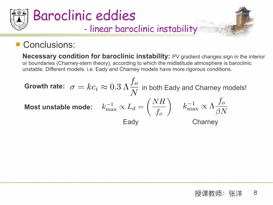
n Conclusions: Necessary condition for baroclinic instability: PV gradient changes sign in the interior or boundaries (Charney-stern theory), according to which the midlatitude atmosphere is baroclinic unstable. Different models. i.e. Eady and Charney models have more rigorous conditions.

� = kci

⇡ 0.3 ⇤fo

NGrowth rate: in both Eady and Charney models!

k�1

max

/ ⇤fo

�NMost unstable mode:

Eady Charney

k�1

max

/ Ld

=

✓NH

fo

◆



n Conclusions:

n Discussion n Normal mode assumption

n Small amplitude assumption, linearization n Assumption: uniform vertical shear of the zonal flow

Necessary condition for baroclinic instability: PV gradient changes sign in the interior or boundaries (Charney-stern theory), according to which the midlatitude atmosphere is baroclinic unstable. Different models. i.e. Eady and Charney models have more rigorous conditions.

� = kci

⇡ 0.3 ⇤fo

NGrowth rate: in both Eady and Charney models!

k�1

max

/ ⇤fo

�NMost unstable mode:

Eady Charney


Baroclinic eddies - baroclinic eddy life cycle

Numerical simulations with idealized GCM:

Basic state at the initial moment: close to real atmosphere.

temperature

Jet (Thorncroft et al, 1993, Q.J.R.)

Results: Capture the synoptic feature of baroclinic eddies.



n Eddies’ development

(Thorncroft et al, 1993, Q.J.R.)

Small amplitude perturbations

Finite amplitude perturbations

Wave breaking



n Mean flow adjustment

at day 9

Numerical results from

Gutowski et al, 1989, JAS, where F and H indicate simulations with

friction, diabatic heating, respectively

Much more stable stratification in the lower

troposphere.

Weaker vertical shear mean reduced

temperature gradient.



n Westerly jet and energy cycle:

Numerical results from Simmons and Hoskins,

1978, JAS

ii

ii

ii

ii

4

3

2

1

0

-3

-2

-1

Wm

-2

0 2 64 12 148 10

50

40

30

-1

0 3 6 9 12 15 (days)

C(AZ AE)

C(AE KE)

C(AZ KZ)

C(KZ KE)

time

u (m

s

)En

ergy

con

vers

ions

Fig. 9.9 Top: energy conversion and dissipation processes in a numerical simulationof an idealized atmospheric baroclinic lifecycle, simulated with a GCM. Bottom: evo-lution of the maximum zonal-mean velocity. AZ and AE are zonal and eddy availablepotential energies, and KZ and KE are the corresponding kinetic energies. Initiallybaroclinic processes dominate, with conversions from zonal to eddy kinetic energyand then eddy kinetic to eddy available potential energy, followed by the barotropicconversion of eddy kinetic to zonal kinetic energy. The latter process is reflected inthe increase of the maximum zonal-mean velocity at about day 10.6

From Vallis (2006)

From Vallis (2006)

Strengthen of westerly jet


Baroclinic eddies

n From linear to nonlinear

Basic flow or

Pre-existing flow (without zonal variation and baroclinic unstable)

Small perturbation

Perturbations grow with time

(finite amplitude pert.)Eddy-mean interactions

(Adjust the zonal flow)

Equilibrated states between the adjusted zonal flow and baroclinic eddies

Linear process

Nonlinear interactions

Reduce the zonal flow temperature gradient; stablize the lower level

stratification; enhance the westerly jet

0 100 200 300 400 500 60040

50

60

70

80

90

100Time series of KE for SD run

MK

E (×

105 J

/m2 )

0 100 200 300 400 500 6000

5

10

15

20

25

30

EK

E (×

105 J

/m2 )

0 100 200 300 400 500 600

200

400

day

Time series of PE for SD run

MPE

(× 1

05 J/m

2 )

0 100 200 300 400 500 6000

20

40

EPE

(× 1

05 J/m

2 )

Numerical results from a QG model (Zhang, 2009)


Baroclinic eddies


Basic flow or


Small perturbation





EquilibriumNonlinear adjustment

spinup of eddies

0 100 200 300 400 500 60040

50

60

70

80

90

100Time series of KE for SD run

MK

E (×

105 J

/m2 )

0 100 200 300 400 500 6000

5

10

15

20

25

30

EK

E (×

105 J

/m2 )

0 100 200 300 400 500 600

200

400

day

Time series of PE for SD run

MPE

(× 1

05 J/m

2 )

0 100 200 300 400 500 6000

20

40

EPE

(× 1

05 J/m

2 )

Numerical results from a QG model (Zhang, 2009)


Baroclinic eddies


Basic flow or


Small perturbation





EquilibriumNonlinear adjustment

spinup of eddies

E-P flux


Outline

n Observations

n The Ferrel Cell

n Baroclinic eddies n Review: baroclinic instability and baroclinic eddy life cycle

n Eddy-mean flow interaction, E-P flux

n Transformed Eulerian Mean equations

n Eddy-driven jet

n The energy cycle


n Start from the equations:


A = [A] +A⇤Decompose into zonal mean and eddy components:

n Momentum equation:✓du

dt

◆

p

� fv = �✓@�

@x

◆

p

+ F

x

✓d ln ✓

dt

◆

p

=Q

cpT

rp · v +@!

@p= 0n Continuity equation:

n Thermodynamic equation:

✓d

dt

◆

p

=

✓@

@t

◆

p

+ u

✓@

@x

◆

p

+ v

✓@

@y

◆

p

+ !

@

@p

@[v]

@y+

@[!]

@p= 0

Under the quasi-geostrophic approximation (Ro

⌧ 1)

@[u]

@t= �@([u⇤v⇤])

@y+ f [v] + [F

x

]

@[✓]

@t+ [!]

@✓s

@p= �@([✓⇤v⇤])

@y+

✓po

p

◆R/cp [Q]

cp



✓d

dt

◆

p

=

✓@

@t

◆

p

+ u

✓@

@x

◆

p

+ v

✓@

@y

◆

p

+ !

@

@p

n Momentum equation:

n Continuity equation:


n The simplified equations:


Baroclinic eddies - E-P flux

@[v]

@y+

@[!]

@p= 0

@[u]

@t= �@([u⇤v⇤])

@y+ f [v] + [F

x

]

@[✓]

@t+ [!]

@✓s

@p= �@([✓⇤v⇤])

@y+

✓po

p

◆R/cp [Q]

cp




n In a steady, adiabatic and frictionless flow:

f [v]�@([u⇤v⇤])

@y= 0

[!]@✓s@p

+@([✓⇤v⇤])

@y= 0

[!] = � @

@y

✓[✓⇤v⇤]

@✓s/@p

◆

[v] =1

f

@

@y([u⇤v⇤])

F ⌘ �[u⇤v⇤] j+ f[v⇤✓⇤]

@✓s/@pk

r · F = 0



@[v]

@y+

@[!]

@p= 0




n In a QG, steady, adiabatic and frictionless flow:

Define Eliassen-Palm flux:

[!] = � @

@y

✓[✓⇤v⇤]

@✓s/@p

◆[v] =

1

f

@

@y([u⇤v⇤])

F ⌘ �[u⇤v⇤] j+ f[v⇤✓⇤]

@✓s/@pk

r · F = 0

f [v]�@([u⇤v⇤])

@y+ [F

x

] = 0

[!]@✓

s

@p+

@([✓⇤v⇤])

@y�✓po

p

◆R/cp [Q]

cp

= 0



n In a QG, steady, adiabatic and frictionless flow:

n In a QG, steady flow:

The meridional overturning flow, in addition to the eddy forcing, has to balance the external forcing.

f [v]�@([u⇤v⇤])

@y+ [F

x

] = 0

[!]@✓

s

@p+

@([✓⇤v⇤])

@y�✓po

p

◆R/cp [Q]

cp

= 0

˜[!] = [!] +@

@y

✓[v⇤✓⇤]

@✓s/@p

◆

˜[v] = [v]� @

@p

✓[v⇤✓⇤]

@✓s/@p

◆

@ ˜[v]

@y+

@ ˜[!]

@p= 0



n In a QG, steady flow:

Define:

Residual mean meridional circulation

F ⌘ �[u⇤v⇤] j+ f[v⇤✓⇤]

@✓s/@pk

@[u]

@t= f ˜[v] +r · F + [F

x

]

@[✓]

@t= � ˜[!]

@✓s

@p+

✓po

p

◆R/cp [Q]

cp

0

0

@[✓]

@t= � ˜[!]

@✓s

@p+

✓po

p

◆R/cp [Q]

cp

@ ˜[v]

@y+

@ ˜[!]

@p= 0



n In a QG flow:

Define:

Residual mean meridional circulation

F ⌘ �[u⇤v⇤] j+ f[v⇤✓⇤]

@✓s/@pk

(Quasi-geostrophic) Transformed Eulerian mean equations

@[u]

@t= f ˜[v] +r · F + [F

x

]

0

0

˜[!] = [!] +@

@y

✓[v⇤✓⇤]

@✓s/@p

◆

˜[v] = [v]� @

@p

✓[v⇤✓⇤]

@✓s/@p

◆

f [v]�@([u⇤v⇤])

@y+ [F

x

] = 0

[!]@✓

s

@p+

@([✓⇤v⇤])

@y�✓po

p

◆R/cp [Q]

cp

= 0

( ˜[v], ˜[!]) =

�@ @p

,@

@y

!

= m +[v⇤✓⇤]

@✓s/@p


Baroclinic eddies - TEM

@[✓]

@t= � ˜[!]

@✓s

@p+

✓po

p

◆R/cp [Q]

cp

@[u]

@t= f ˜[v] +r · F + [F

x

]

@ ˜[v]

@y+

@ ˜[!]

@p= 0

˜[!] = [!] +@

@y

✓[v⇤✓⇤]

@✓s/@p

◆

˜[v] = [v]� @

@p

✓[v⇤✓⇤]

@✓s/@p

◆

Recall the streamfunction for the zonal mean flow:

Define a streamfunction for the residual mean circulation:

([v], [!]) =

✓�@ m

@p,@ m

@y

◆



Case 1: The EADY model

ii

ii

ii

ii

(Eulerian)

0 0.25 0.5 0.75 10

0.5

1

(Residual)

Latitude (y/L)

Hei

ght

(z/D

)

0 0.25 0.5 0.75 10

0.5

1

Hei

ght

(z/D

)

ψE

ψ *

Fig. 7.3 The Eulerian streamfunction (top) and the residual streamfunction for theEady problem, calculated using (7.135) and (7.136), with L2/L2

d = 9.

From Vallis (2006)

From Vallis (2006)

= m +[v⇤✓⇤]

@✓s/@p

The residual mean circulation’s direction can be opposite to the Eulerian mean circulation.

(x, y, z) , (x, y, ✓)

D✓

Dt= ✓

D

Dt=

@

@t+ u ·r✓ +

D✓

Dt

@

@✓

=@

@t+ u ·r✓ + ✓

@

@✓


n In isentropic coordinate

The Ferrel Cell

zero for adiabatic flow

Isentrope: An isopleth of entropy. In meteorology it is usually identified with an isopleth of potential temperature.

Case 2: Observed circulation


The Ferrel Cell

(Fig.11.4, Vallis, 2006)

The direction of Ferrel cell is reversed in the isentropic coordinate.


D

Dt=

@

@t+ u ·r✓ +

D✓

Dt

@

@✓

=@

@t+ u ·r✓ + ✓

@

@✓



Case 2: Observed circulation

The Ferrel cell in the isentropic coordinate is essentially reflect the

Residual Mean Circulation. (Fig.11.4, Vallis, 2006)


D

Dt=

@

@t+ u ·r✓ +

D✓

Dt

@

@✓

=@

@t+ u ·r✓ + ✓

@

@✓

zero for adiabatic flow

= m +[v⇤✓⇤]

@✓s/@p


Baroclinic eddies


Basic flow or


Small perturbation





Linear process

Nonlinear interactions

E-P flux, residual mean circulation,

Transformed Eulerian mean equations.

v⇣ = v(@v

@x

� @u

@y

)

= � @

@y

uv +1

2

@

@x

(v2 � u

2)q

0 =@

2

0

@x

2+@

2

0

@y

2+ f

2o

@

@p

✓1

s

@

0

@p

◆

q =@2

@y2+ �y + f2

o

@

@p

✓1

s

@

@p

◆v0q0 = v0⇣ 0 +

fo

@✓s

/@pv0@✓0

@p

v@✓

@p=

@

@pv✓ � ✓

@v

@p

(u, v) =

✓�@ @y

,

@

@x

◆✓ = �f

o

@

@p

=p

R

✓po

p

◆R/cp

s = � 1

@✓s@p

v

@✓

@p

=@

@p

v✓ +1

2fo

@

@x

✓

2


Baroclinic eddies - E-P flux: a second view

n E-P flux and the Quasi-geostrophic potential vorticity

F ⌘ �[u⇤v⇤] j+ f[v⇤✓⇤]

@✓s/@pk

From the definition of QG potential vorticity:

⇣ 0 fo

@

@p

✓✓0

@✓s

/@p

◆

PV flux:

thermal wind relation for

meridional wind

+✓

f

o

@✓

@x

Note: ‘ denotes small perturbation

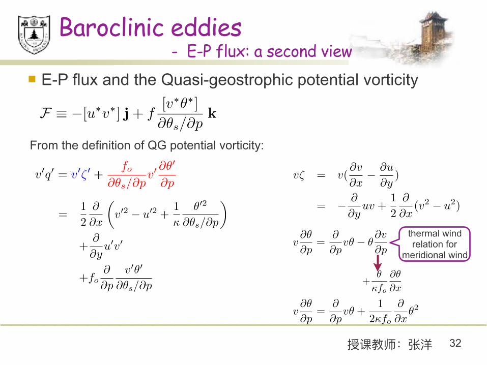
v0q0 = v0⇣ 0 +fo

@✓s

/@pv0@✓0

@p

=1

2

@

@x

✓v

02 � u

02 +1

✓

02

@✓

s

/@p

◆

+@

@y

u

0v

0

+f

o

@

@p

v

0✓

0

@✓

s

/@p



F ⌘ �[u⇤v⇤] j+ f[v⇤✓⇤]

@✓s/@pk


v⇣ = v(@v

@x

� @u

@y

)

= � @

@y

uv +1

2

@

@x

(v2 � u

2)

v@✓

@p=

@

@pv✓ � ✓

@v

@p

+✓

f

o

@✓

@x

v

@✓

@p

=@

@p

v✓ +1

2fo

@

@x

✓

2

thermal wind relation for

meridional wind


[v⇤q⇤] =@

@y[u⇤v⇤] + f

o

@

@p

[v⇤✓⇤]

@✓s

/@p

= r · F



F ⌘ �[u⇤v⇤] j+ f[v⇤✓⇤]

@✓s/@pk


v0q0 = v0⇣ 0 +fo

@✓s

/@pv0@✓0

@p

=1

2

@

@x

✓v

02 � u

02 +1

✓

02

@✓

s

/@p

◆

+@

@y

u

0v

0

+f

o

@

@p

v

0✓

0

@✓

s

/@p

Zonally averaged PV flux by eddies:


#1

✓@

@t

+ U

@

@x

◆q

0 +@

0

@x

@q

@y

= 0

1

2

@

@t[q02] + [v0q0]

@q

@y= 0

A =[q02]

2@q/@y

@A@t

+r · F = 0


n E-P flux and the Eliassen-Palm relation

F ⌘ �[u⇤v⇤] j+ f[v⇤✓⇤]

@✓s/@pk


Multiplying by q’ and zonally average:

Define wave activity density:

Eliassen-Palm relation


#2

✓@

@t

+ U

@

@x

◆q

0 +@

0

@x

@q

@y

= 0

Assume U is fixed, and

@q

@y= �

✓@

@t

+ U

@

@x

◆r2

0 + f

2o

@

@p

✓1

s

@

0

@p

◆�+ �

@

0

@x

= 0

0 = Re ei(kx+ly+mp�!t)

! = Uk � �k

K2

K2 = k2 + l2 +m2f2o

/s

A0 = ReAei(kx+ly+mp�!t)

✓ = �Reimfo

, q = �ReK2

cgy =2�kl

K4cgp

=2�kmf2

o

/s

K4

u = �Reil , v = Reik


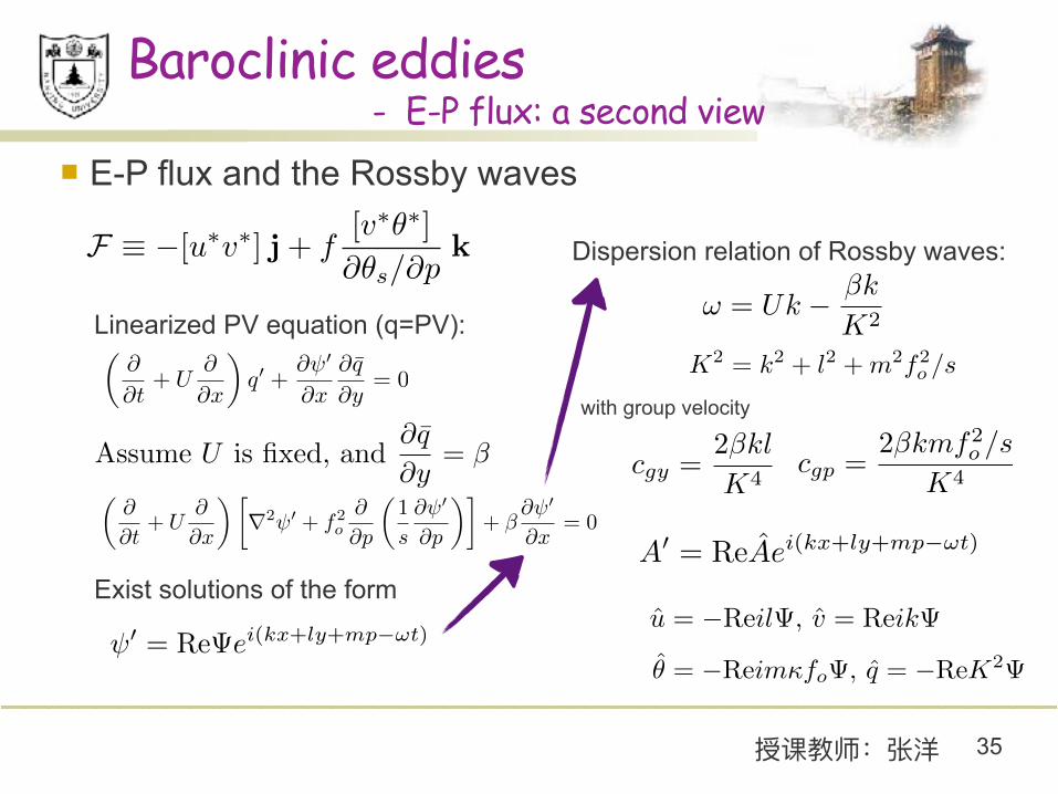
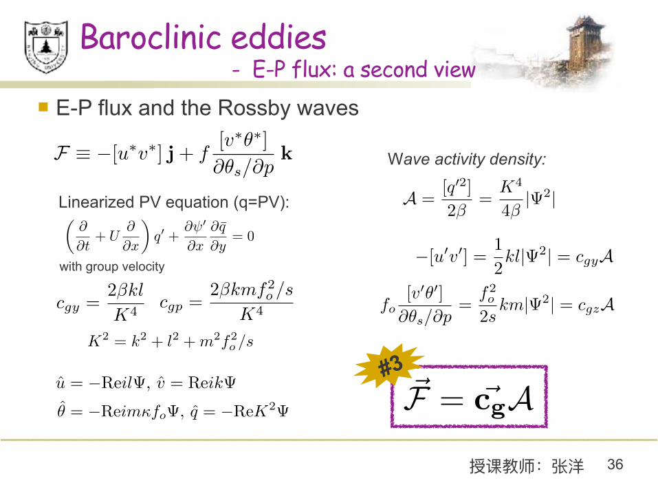
n E-P flux and the Rossby waves

F ⌘ �[u⇤v⇤] j+ f[v⇤✓⇤]

@✓s/@pk


Exist solutions of the form

Dispersion relation of Rossby waves:

with group velocity


✓@

@t

+ U

@

@x

◆q

0 +@

0

@x

@q

@y

= 0

K2 = k2 + l2 +m2f2o

/s

✓ = �Reimfo

, q = �ReK2

A =[q02]

2�=

K4

4�| 2|

~F = ~cgA

�[u0v0] =1

2kl| 2| = cgyA

fo

[v0✓0]

@✓s

/@p=

f2o

2skm| 2| = c

gz

A


n E-P flux and the Rossby waves

F ⌘ �[u⇤v⇤] j+ f[v⇤✓⇤]

@✓s/@pk


with group velocity

Wave activity density:


#3

cgy =2�kl

K4cgp

=2�kmf2

o

/s

K4

u = �Reil , v = Reik

@A@t

+r · (A ~cg) = 0


E-P flux, TEM and Residual Circulation - Summary

n E-P flux: F ⌘ �[u⇤v⇤] j+ f[v⇤✓⇤]

@✓s/@pk

n TEM equations:

#1 [v⇤q⇤] =@

@y[u⇤v⇤] + f

o

@

@p

[v⇤✓⇤]

@✓s

/@p

= r · F

~F = ~cgA#3

n Residual mean circulations:

#2 @A@t

+r · F = 0

n In a steady, adiabatic and frictionless flow:

@[✓]

@t= � ˜[!]

@✓s

@p+

✓po

p

◆R/cp [Q]

cp

@[u]

@t= f ˜[v] +r · F + [F

x

] ,

˜[!] = [!] +@

@y

✓[v⇤✓⇤]

@✓s/@p

◆˜[v] = [v]� @

@p

✓[v⇤✓⇤]

@✓s/@p

◆

,

r · F = 0[!] = � @

@y

✓[✓⇤v⇤]

@✓s/@p

◆[v] =

1

f

@

@y([u⇤v⇤])

chap 4 3 2021 - tcs.nju.edu.cn

Documents