chap-14 (14th nov.) · solution: recall that to find the mean marks, we require the product of each...

260 MATHEMATICS

1414.1 Introduction

In Class IX, you have studied the classification of given data into ungrouped as well as

grouped frequency distributions. You have also learnt to represent the data pictorially

in the form of various graphs such as bar graphs, histograms (including those of varying

widths) and frequency polygons. In fact, you went a step further by studying certain

numerical representatives of the ungrouped data, also called measures of central

tendency, namely, mean, median and mode. In this chapter, we shall extend the study

of these three measures, i.e., mean, median and mode from ungrouped data to that of

grouped data. We shall also discuss the concept of cumulative frequency, the

cumulative frequency distribution and how to draw cumulative frequency curves, called

ogives.

14.2 Mean of Grouped Data

The mean (or average) of observations, as we know, is the sum of the values of all the

observations divided by the total number of observations. From Class IX, recall that if

x1, x

2,. . ., x

n are observations with respective frequencies f

1, f

2, . . ., f

n, then this

means observation x1 occurs f

1 times, x

2 occurs f

2 times, and so on.

Now, the sum of the values of all the observations = f1x

1 + f

2x

2 + . . . + f

nx

n, and

the number of observations = f1 + f

2 + . . . + f

n.

So, the mean x of the data is given by

x =1 1 2 2

1 2

n n

n

f x f x f x

f f f

+ + +

+ + +

�

�

Recall that we can write this in short form by using the Greek letter Σ (capital

sigma) which means summation. That is,

STATISTICS

2019-20

STATISTICS 261

x =1

1

n

i i

i

n

i

i

f x

f

=

=

∑

∑

which, more briefly, is written as x = Σ

Σ

i i

i

f x

f, if it is understood that i varies from

1 to n.

Let us apply this formula to find the mean in the following example.

Example 1 : The marks obtained by 30 students of Class X of a certain school in a

Mathematics paper consisting of 100 marks are presented in table below. Find the

mean of the marks obtained by the students.

Marks obtained 10 20 36 40 50 56 60 70 72 80 88 92 95

(xi)

Number of 1 1 3 4 3 2 4 4 1 1 2 3 1

students ( fi)

Solution: Recall that to find the mean marks, we require the product of each xi with

the corresponding frequency fi. So, let us put them in a column as shown in Table 14.1.

Table 14.1

Marks obtained (xi) Number of students ( f

i) f

ix

i

10 1 10

20 1 20

. 36 3 108

40 4 160

50 3 150

56 2 112

60 4 240

70 4 280

72 1 72

80 1 80

88 2 176

92 3 276

95 1 95

Total Σfi = 30 Σf

ix

i = 1779

2019-20

262 MATHEMATICS

Now, Σ

=Σ

i i

i

f xx

f =

1779

30 = 59.3

Therefore, the mean marks obtained is 59.3.

In most of our real life situations, data is usually so large that to make a meaningful

study it needs to be condensed as grouped data. So, we need to convert given ungrouped

data into grouped data and devise some method to find its mean.

Let us convert the ungrouped data of Example 1 into grouped data by forming

class-intervals of width, say 15. Remember that, while allocating frequencies to each

class-interval, students falling in any upper class-limit would be considered in the next

class, e.g., 4 students who have obtained 40 marks would be considered in the class-

interval 40-55 and not in 25-40. With this convention in our mind, let us form a grouped

frequency distribution table (see Table 14.2).

Table 14.2

Class interval 10 - 25 25 - 40 40 - 55 55 - 70 70 - 85 85 - 100

Number of students 2 3 7 6 6 6

Now, for each class-interval, we require a point which would serve as the

representative of the whole class. It is assumed that the frequency of each class-

interval is centred around its mid-point. So the mid-point (or class mark) of each

class can be chosen to represent the observations falling in the class. Recall that we

find the mid-point of a class (or its class mark) by finding the average of its upper and

lower limits. That is,

Class mark =Upper class limit + Lower class limit

2

With reference to Table 14.2, for the class 10-25, the class mark is 10 25

2

+, i.e.,

17.5. Similarly, we can find the class marks of the remaining class intervals. We put

them in Table 14.3. These class marks serve as our xi’s. Now, in general, for the ith

class interval, we have the frequency fi corresponding to the class mark x

i. We can

now proceed to compute the mean in the same manner as in Example 1.

2019-20

STATISTICS 263

Table 14.3

Class interval Number of students ( fi) Class mark (x

i) f

ix

i

10 - 25 2 17.5 35.0

25 - 40 3 32.5 97.5

40 - 55 7 47.5 332.5

55 - 70 6 62.5 375.0

70 - 85 6 77.5 465.0

85 - 100 6 92.5 555.0

Total Σ fi = 30 Σ f

ix

i = 1860.0

The sum of the values in the last column gives us Σ fix

i. So, the mean x of the

given data is given by

x =1860.0

6230

i i

i

f x

f

Σ= =

Σ

This new method of finding the mean is known as the Direct Method.

We observe that Tables 14.1 and 14.3 are using the same data and employing the

same formula for the calculation of the mean but the results obtained are different.

Can you think why this is so, and which one is more accurate? The difference in the

two values is because of the mid-point assumption in Table 14.3, 59.3 being the exact

mean, while 62 an approximate mean.

Sometimes when the numerical values of xi and f

i are large, finding the product

of xi and f

i becomes tedious and time consuming. So, for such situations, let us think of

a method of reducing these calculations.

We can do nothing with the fi’s, but we can change each x

i to a smaller number

so that our calculations become easy. How do we do this? What about subtracting a

fixed number from each of these xi’s? Let us try this method.

The first step is to choose one among the xi’s as the assumed mean, and denote

it by ‘a’. Also, to further reduce our calculation work, we may take ‘a’ to be that xi

which lies in the centre of x1, x

2, . . ., x

n. So, we can choose a = 47.5 or a = 62.5. Let

us choose a = 47.5.

The next step is to find the difference di between a and each of the x

i’s, that is,

the deviation of ‘a’ from each of the xi’s.

i.e., di = x

i – a = x

i – 47.5

2019-20

264 MATHEMATICS

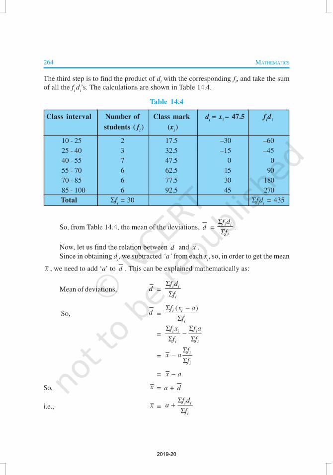
The third step is to find the product of di with the corresponding f

i, and take the sum

of all the fi d

i’s. The calculations are shown in Table 14.4.

Table 14.4

Class interval Number of Class mark di = x

i – 47.5 f

id

i

students ( fi) (x

i)

10 - 25 2 17.5 –30 –60

25 - 40 3 32.5 –15 –45

40 - 55 7 47.5 0 0

55 - 70 6 62.5 15 90

70 - 85 6 77.5 30 180

85 - 100 6 92.5 45 270

Total Σfi = 30 Σf

id

i = 435

So, from Table 14.4, the mean of the deviations, d = i i

i

f d

f

Σ

Σ.

Now, let us find the relation between d and x .

Since in obtaining di, we subtracted ‘a’ from each x

i, so, in order to get the mean

x , we need to add ‘a’ to d . This can be explained mathematically as:

Mean of deviations, d =i i

i

f d

f

Σ

Σ

So, d =( )i i

i

f x a

f

Σ −

Σ

=i i i

i i

f x f a

f f

Σ Σ−

Σ Σ

=i

i

fx a

f

Σ−

Σ

= x a−

So, x = a + d

i.e., x =i i

i

f da

f

Σ+

Σ

2019-20

STATISTICS 265

Substituting the values of a, Σfid

i and Σf

i from Table 14.4, we get

x =435

47.5 47.5 14.5 6230

+ = + = .

Therefore, the mean of the marks obtained by the students is 62.

The method discussed above is called the Assumed Mean Method.

Activity 1 : From the Table 14.3 find the mean by taking each of xi (i.e., 17.5, 32.5,

and so on) as ‘a’. What do you observe? You will find that the mean determined in

each case is the same, i.e., 62. (Why ?)

So, we can say that the value of the mean obtained does not depend on the

choice of ‘a’.

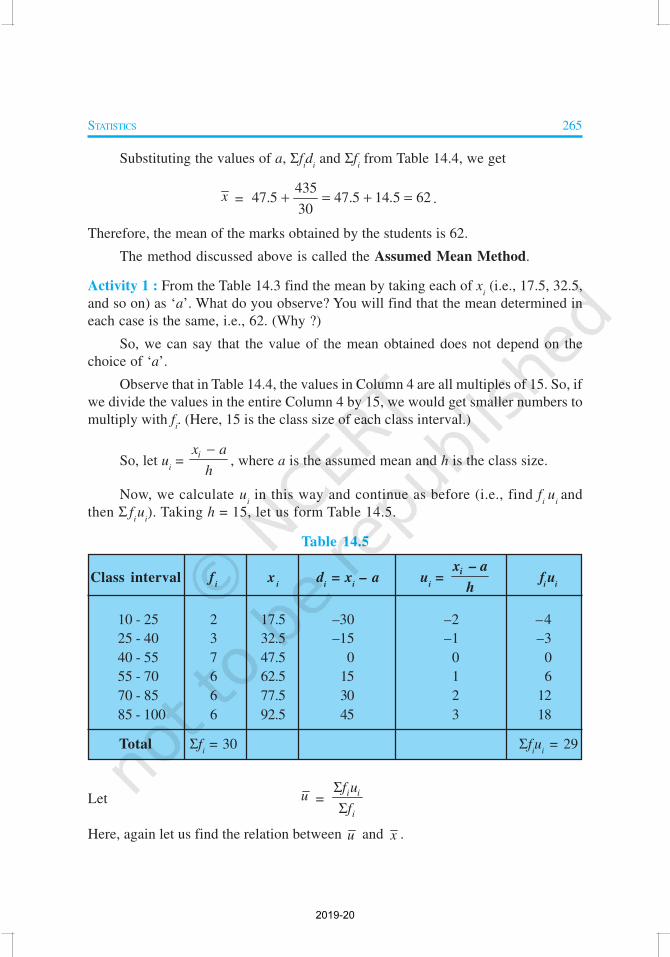
Observe that in Table 14.4, the values in Column 4 are all multiples of 15. So, if

we divide the values in the entire Column 4 by 15, we would get smaller numbers to

multiply with fi. (Here, 15 is the class size of each class interval.)

So, let ui =

ix a

h

−, where a is the assumed mean and h is the class size.

Now, we calculate ui in this way and continue as before (i.e., find f

i u

i and

then Σ fiu

i). Taking h = 15, let us form Table 14.5.

Table 14.5

Class interval fi

xi

di = x

i – a u

i =

ix – a

hfiu

i

10 - 25 2 17.5 –30 –2 –4

25 - 40 3 32.5 –15 –1 –3

40 - 55 7 47.5 0 0 0

55 - 70 6 62.5 15 1 6

70 - 85 6 77.5 30 2 12

85 - 100 6 92.5 45 3 18

Total Σfi = 30 Σf

iu

i = 29

Let u =i i

i

f u

f

Σ

Σ

Here, again let us find the relation between u and x .

2019-20

266 MATHEMATICS

We have, ui =

ix a

h

−

Therefore, u =

( )

1i

ii i i

i i

x af

f x a fh

f h f

−Σ Σ − Σ

= Σ Σ

=1 i i i

i i

f x fa

h f f

Σ Σ−

Σ Σ

= [ ]1

x ah

−

So, hu = x a−

i.e., x = a + hu

So, x =i i

i

f ua h

f

Σ+

Σ

Now, substituting the values of a, h, Σfiu

i and Σf

i from Table 14.5, we get

x =29

47.5 1530

+ ×

= 47.5 + 14.5 = 62

So, the mean marks obtained by a student is 62.

The method discussed above is called the Step-deviation method.

We note that :

l the step-deviation method will be convenient to apply if all the di’s have a

common factor.

l The mean obtained by all the three methods is the same.

l The assumed mean method and step-deviation method are just simplified

forms of the direct method.

l The formula x = a + hu still holds if a and h are not as given above, but are

any non-zero numbers such that ui =

ix a

h

−.

Let us apply these methods in another example.

2019-20

STATISTICS 267

Example 2 : The table below gives the percentage distribution of female teachers in

the primary schools of rural areas of various states and union territories (U.T.) of

India. Find the mean percentage of female teachers by all the three methods discussed

in this section.

Percentage of 15 - 25 25 - 35 35 - 45 45 - 55 55 - 65 65 - 75 75 - 85

female teachers

Number of 6 11 7 4 4 2 1

States/U.T.

Source : Seventh All India School Education Survey conducted by NCERT

Solution : Let us find the class marks, xi, of each class, and put them in a column

(see Table 14.6):

Table 14.6

Percentage of female Number of xi

teachers States /U.T. ( fi)

15 - 25 6 20

25 - 35 11 30

35 - 45 7 40

45 - 55 4 50

55 - 65 4 60

65 - 75 2 70

75 - 85 1 80

Here we take a = 50, h = 10, then di = x

i – 50 and

50

10

i

i

xu

−= .

We now find diand u

i and put them in Table 14.7.

2019-20

268 MATHEMATICS

Table 14.7

Percentage of Number of xi

di = x

i – 50 −50

=10

ii

xu f

ix

ifid

ifiu

i

female states/U.T.

teachers ( fi)

15 - 25 6 20 –30 –3 120 –180 –18

25 - 35 11 30 –20 –2 330 –220 –22

35 - 45 7 40 –10 –1 280 –70 –7

45 - 55 4 50 0 0 200 0 0

55 - 65 4 60 10 1 240 40 4

65 - 75 2 70 20 2 140 40 4

75 - 85 1 80 30 3 80 30 3

Total 35 1390 –360 –36

From the table above, we obtain Σfi = 35, Σf

ix

i = 1390,

Σfid

i = – 360, Σf

iu

i = –36.

Using the direct method, 1390

39.7135

Σ= = =

Σ

i i

i

f xx

f

Using the assumed mean method,

x =i i

i

f da

f

Σ+

Σ =

( 360)50 39.71

35

−+ =

Using the step-deviation method,

x =– 36

50 10 39.7135

i i

i

f ua h

f

Σ + × = + × =

Σ

Therefore, the mean percentage of female teachers in the primary schools of

rural areas is 39.71.

Remark : The result obtained by all the three methods is the same. So the choice of

method to be used depends on the numerical values of xi and f

i. If x

i and f

i are

sufficiently small, then the direct method is an appropriate choice. If xi and f

i are

numerically large numbers, then we can go for the assumed mean method or

step-deviation method. If the class sizes are unequal, and xi are large numerically, we

can still apply the step-deviation method by taking h to be a suitable divisor of all the di’s.

2019-20

STATISTICS 269

Example 3 : The distribution below shows the number of wickets taken by bowlers in

one-day cricket matches. Find the mean number of wickets by choosing a suitable

method. What does the mean signify?

Number of 20 - 60 60 - 100 100 - 150 150 - 250 250 - 350 350 - 450

wickets

Number of 7 5 16 12 2 3

bowlers

Solution : Here, the class size varies, and the xi

,s are large. Let us still apply the step-

deviation method with a = 200 and h = 20. Then, we obtain the data as in Table 14.8.

Table 14.8

Number of Number of xi

di = x

i – 200 =

20

ii

du u

if

i

wickets bowlers

taken ( fi)

20 - 60 7 40 –160 –8 –56

60 - 100 5 80 –120 –6 –30

100 - 150 16 125 –75 –3.75 –60

150 - 250 12 200 0 0 0

250 - 350 2 300 100 5 10

350 - 450 3 400 200 10 30

Total 45 –106

So, 106

45

−= ⋅u Therefore, x = 200 +

10620

45

−

= 200 – 47.11 = 152.89.

This tells us that, on an average, the number of wickets taken by these 45 bowlers

in one-day cricket is 152.89.

Now, let us see how well you can apply the concepts discussed in this section!

2019-20

270 MATHEMATICS

Activity 2 :

Divide the students of your class into three groups and ask each group to do one of the

following activities.

1. Collect the marks obtained by all the students of your class in Mathematics in the

latest examination conducted by your school. Form a grouped frequency distribution

of the data obtained.

2. Collect the daily maximum temperatures recorded for a period of 30 days in your

city. Present this data as a grouped frequency table.

3. Measure the heights of all the students of your class (in cm) and form a grouped

frequency distribution table of this data.

After all the groups have collected the data and formed grouped frequency

distribution tables, the groups should find the mean in each case by the method which

they find appropriate.

EXERCISE 14.1

1. A survey was conducted by a group of students as a part of their environment awareness

programme, in which they collected the following data regarding the number of plants in

20 houses in a locality. Find the mean number of plants per house.

Number of plants 0 - 2 2 - 4 4 - 6 6 - 8 8 - 10 10 - 12 12 - 14

Number of houses 1 2 1 5 6 2 3

Which method did you use for finding the mean, and why?

2. Consider the following distribution of daily wages of 50 workers of a factory.

Daily wages (in ̀ ) 500 - 520 520 -540 540 - 560 560 - 580 580 -600

Number of workers 12 14 8 6 10

Find the mean daily wages of the workers of the factory by using an appropriate method.

3. The following distribution shows the daily pocket allowance of children of a locality.

The mean pocket allowance is Rs 18. Find the missing frequency f.

Daily pocket 11 - 13 13 - 15 15 - 17 17 - 19 19 - 21 21 - 23 23 - 25

allowance (in ̀ )

Number of children 7 6 9 13 f 5 4

2019-20

STATISTICS 271

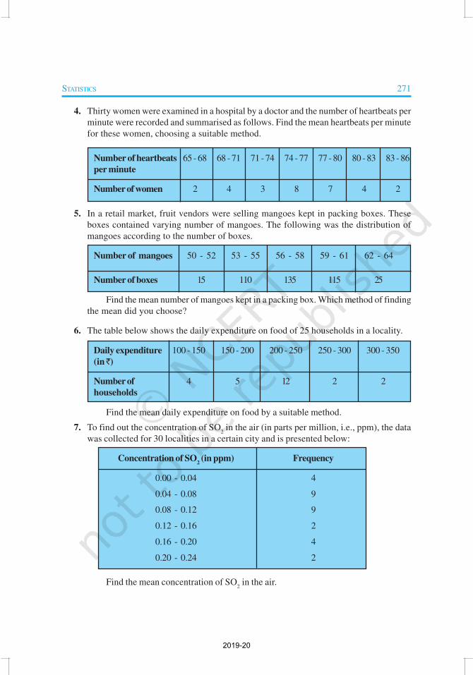
4. Thirty women were examined in a hospital by a doctor and the number of heartbeats per

minute were recorded and summarised as follows. Find the mean heartbeats per minute

for these women, choosing a suitable method.

Number of heartbeats 65 - 68 68 - 71 71 - 74 74 - 77 77 - 80 80 - 83 83 - 86

per minute

Number of women 2 4 3 8 7 4 2

5. In a retail market, fruit vendors were selling mangoes kept in packing boxes. These

boxes contained varying number of mangoes. The following was the distribution of

mangoes according to the number of boxes.

Number of mangoes 50 - 52 53 - 55 56 - 58 59 - 61 62 - 64

Number of boxes 15 110 135 115 25

Find the mean number of mangoes kept in a packing box. Which method of finding

the mean did you choose?

6. The table below shows the daily expenditure on food of 25 households in a locality.

Daily expenditure 100 - 150 150 - 200 200 - 250 250 - 300 300 - 350

(in ̀ )

Number of 4 5 12 2 2

households

Find the mean daily expenditure on food by a suitable method.

7. To find out the concentration of SO2 in the air (in parts per million, i.e., ppm), the data

was collected for 30 localities in a certain city and is presented below:

Concentration of SO2 (in ppm) Frequency

0.00 - 0.04 4

0.04 - 0.08 9

0.08 - 0.12 9

0.12 - 0.16 2

0.16 - 0.20 4

0.20 - 0.24 2

Find the mean concentration of SO2 in the air.

2019-20

272 MATHEMATICS

8. A class teacher has the following absentee record of 40 students of a class for the whole

term. Find the mean number of days a student was absent.

Number of 0 - 6 6 - 10 10 - 14 14 - 20 20 - 28 28 - 38 38 - 40

days

Number of 11 10 7 4 4 3 1

students

9. The following table gives the literacy rate (in percentage) of 35 cities. Find the mean

literacy rate.

Literacy rate (in %) 45 - 55 55 - 65 65 - 75 75 - 85 85 - 95

Number of cities 3 10 11 8 3

14.3 Mode of Grouped Data

Recall from Class IX, a mode is that value among the observations which occurs most

often, that is, the value of the observation having the maximum frequency. Further, we

discussed finding the mode of ungrouped data. Here, we shall discuss ways of obtaining

a mode of grouped data. It is possible that more than one value may have the same

maximum frequency. In such situations, the data is said to be multimodal. Though

grouped data can also be multimodal, we shall restrict ourselves to problems having a

single mode only.

Let us first recall how we found the mode for ungrouped data through the following

example.

Example 4 : The wickets taken by a bowler in 10 cricket matches are as follows:

2 6 4 5 0 2 1 3 2 3

Find the mode of the data.

Solution : Let us form the frequency distribution table of the given data as follows:

Number of 0 1 2 3 4 5 6

wickets

Number of 1 1 3 2 1 1 1

matches

2019-20

STATISTICS 273

Clearly, 2 is the number of wickets taken by the bowler in the maximum number

(i.e., 3) of matches. So, the mode of this data is 2.

In a grouped frequency distribution, it is not possible to determine the mode by

looking at the frequencies. Here, we can only locate a class with the maximum

frequency, called the modal class. The mode is a value inside the modal class, and is

given by the formula:

Mode = 1 0

1 0 22

f fl h

f f f

−+ ×

− −

where l = lower limit of the modal class,

h = size of the class interval (assuming all class sizes to be equal),

f1 = frequency of the modal class,

f0 = frequency of the class preceding the modal class,

f2 = frequency of the class succeeding the modal class.

Let us consider the following examples to illustrate the use of this formula.

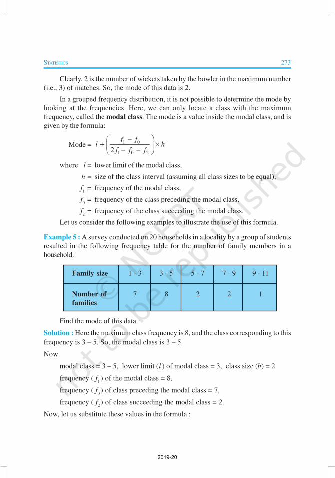
Example 5 : A survey conducted on 20 households in a locality by a group of students

resulted in the following frequency table for the number of family members in a

household:

Family size 1 - 3 3 - 5 5 - 7 7 - 9 9 - 11

Number of 7 8 2 2 1

families

Find the mode of this data.

Solution : Here the maximum class frequency is 8, and the class corresponding to this

frequency is 3 – 5. So, the modal class is 3 – 5.

Now

modal class = 3 – 5, lower limit (l ) of modal class = 3, class size (h) = 2

frequency ( f1) of the modal class = 8,

frequency ( f0) of class preceding the modal class = 7,

frequency ( f2) of class succeeding the modal class = 2.

Now, let us substitute these values in the formula :

2019-20

274 MATHEMATICS

Mode = 1 0

1 0 22

f fl h

f f f

−+ ×

− −

=8 7 2

3 2 3 3.2862 8 7 2 7

−+ × = + =

× − −

Therefore, the mode of the data above is 3.286.

Example 6 : The marks distribution of 30 students in a mathematics examination are

given in Table 14.3 of Example 1. Find the mode of this data. Also compare and

interpret the mode and the mean.

Solution : Refer to Table 14.3 of Example 1. Since the maximum number of students

(i.e., 7) have got marks in the interval 40 - 55, the modal class is 40 - 55. Therefore,

the lower limit ( l ) of the modal class = 40,

the class size ( h) = 15,

the frequency ( f1) of modal class = 7,

the frequency ( f0) of the class preceding the modal class = 3,

the frequency ( f2) of the class succeeding the modal class = 6.

Now, using the formula:

Mode = 1 0

1 0 22

f fl h

f f f

−+ ×

− − ,

we get Mode =7 3

40 1514 6 3

−+ ×

− − = 52

So, the mode marks is 52.

Now, from Example 1, you know that the mean marks is 62.

So, the maximum number of students obtained 52 marks, while on an average a

student obtained 62 marks.

Remarks :

1. In Example 6, the mode is less than the mean. But for some other problems it may

be equal or more than the mean also.

2. It depends upon the demand of the situation whether we are interested in finding the

average marks obtained by the students or the average of the marks obtained by most

2019-20

STATISTICS 275

of the students. In the first situation, the mean is required and in the second situation,

the mode is required.

Activity 3 : Continuing with the same groups as formed in Activity 2 and the situations

assigned to the groups. Ask each group to find the mode of the data. They should also

compare this with the mean, and interpret the meaning of both.

Remark : The mode can also be calculated for grouped data with unequal class sizes.

However, we shall not be discussing it.

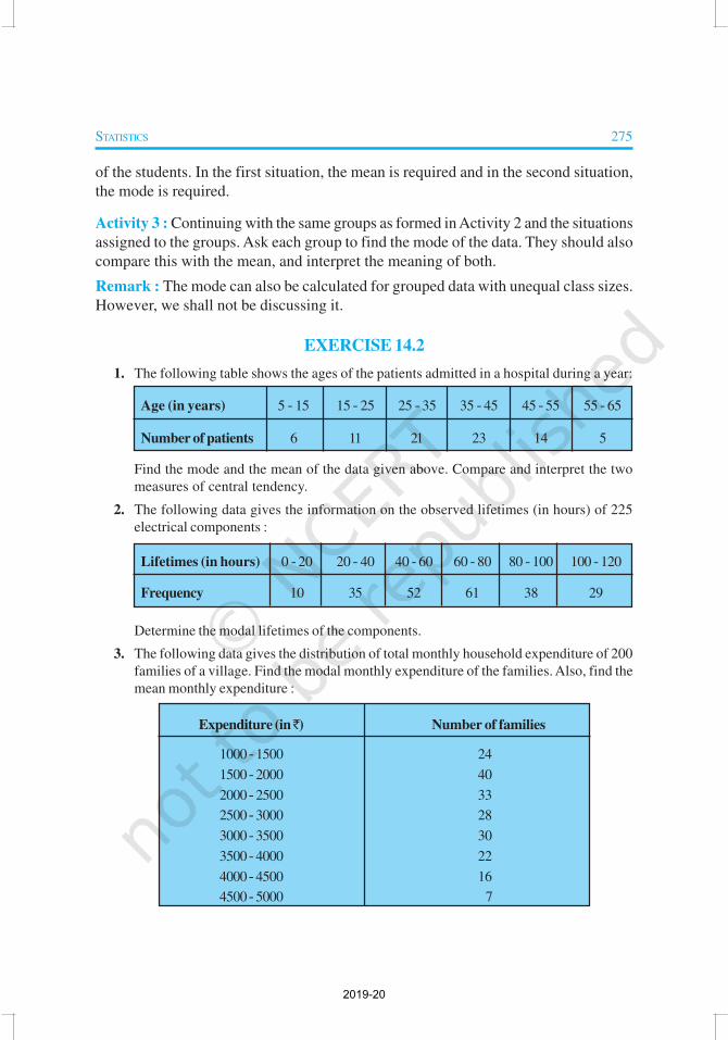
EXERCISE 14.2

1. The following table shows the ages of the patients admitted in a hospital during a year:

Age (in years) 5 - 15 15 - 25 25 - 35 35 - 45 45 - 55 55 - 65

Number of patients 6 11 21 23 14 5

Find the mode and the mean of the data given above. Compare and interpret the two

measures of central tendency.

2. The following data gives the information on the observed lifetimes (in hours) of 225

electrical components :

Lifetimes (in hours) 0 - 20 20 - 40 40 - 60 60 - 80 80 - 100 100 - 120

Frequency 10 35 52 61 38 29

Determine the modal lifetimes of the components.

3. The following data gives the distribution of total monthly household expenditure of 200

families of a village. Find the modal monthly expenditure of the families. Also, find the

mean monthly expenditure :

Expenditure (in ̀ ) Number of families

1000 - 1500 24

1500 - 2000 40

2000 - 2500 33

2500 - 3000 28

3000 - 3500 30

3500 - 4000 22

4000 - 4500 16

4500 - 5000 7

2019-20

276 MATHEMATICS

4. The following distribution gives the state-wise teacher-student ratio in higher

secondary schools of India. Find the mode and mean of this data. Interpret the two

measures.

Number of students per teacher Number of states / U .T.

15 - 20 3

20 - 25 8

25 - 30 9

30 - 35 10

35 - 40 3

40 - 45 0

45 - 50 0

50 - 55 2

5. The given distribution shows the number of runs scored by some top batsmen of the

world in one-day international cricket matches.

Runs scored Number of batsmen

3000 - 4000 4

4000 - 5000 18

5000 - 6000 9

6000 - 7000 7

7000 - 8000 6

8000 - 9000 3

9000 - 10000 1

10000 - 11000 1

Find the mode of the data.

6. A student noted the number of cars passing through a spot on a road for 100

periods each of 3 minutes and summarised it in the table given below. Find the mode

of the data :

Number of cars 0 - 10 10 - 20 20 - 30 30 - 40 40 - 50 50 - 60 60 - 70 70 - 80

Frequency 7 14 13 12 20 11 15 8

2019-20

STATISTICS 277

14.4 Median of Grouped Data

As you have studied in Class IX, the median is a measure of central tendency which

gives the value of the middle-most observation in the data. Recall that for finding the

median of ungrouped data, we first arrange the data values of the observations in

ascending order. Then, if n is odd, the median is the 1

2

n +

th observation. And, if n

is even, then the median will be the average of the th2

nand the 1 th

2

n +

observations.

Suppose, we have to find the median of the following data, which gives the

marks, out of 50, obtained by 100 students in a test :

Marks obtained 20 29 28 33 42 38 43 25

Number of students 6 28 24 15 2 4 1 20

First, we arrange the marks in ascending order and prepare a frequency table as

follows :

Table 14.9

Marks obtained Number of students

(Frequency)

20 6

25 20

28 24

29 28

33 15

38 4

42 2

43 1

Total 100

2019-20

278 MATHEMATICS

Here n = 100, which is even. The median will be the average of the 2

nth and the

12

n +

th observations, i.e., the 50th and 51st observations. To find these

observations, we proceed as follows:

Table 14.10


20 6

upto 25 6 + 20 = 26

upto 28 26 + 24 = 50

upto 29 50 + 28 = 78

upto 33 78 + 15 = 93

upto 38 93 + 4 = 97

upto 42 97 + 2 = 99

upto 43 99 + 1 = 100

Now we add another column depicting this information to the frequency table

above and name it as cumulative frequency column.

Table 14.11

Marks obtained Number of students Cumulative frequency

20 6 6

25 20 26

28 24 50

29 28 78

33 15 93

38 4 97

42 2 99

43 1 100

2019-20

STATISTICS 279

From the table above, we see that:

50th observaton is 28 (Why?)

51st observation is 29

So, Median =28 29

28.52

+=

Remark : The part of Table 14.11 consisting Column 1 and Column 3 is known as

Cumulative Frequency Table. The median marks 28.5 conveys the information that

about 50% students obtained marks less than 28.5 and another 50% students obtained

marks more than 28.5.

Now, let us see how to obtain the median of grouped data, through the following

situation.

Consider a grouped frequency distribution of marks obtained, out of 100, by 53

students, in a certain examination, as follows:

Table 14.12

Marks Number of students

0 - 10 5

10 - 20 3

20 - 30 4

30 - 40 3

40 - 50 3

50 - 60 4

60 - 70 7

70 - 80 9

80 - 90 7

90 - 100 8

From the table above, try to answer the following questions:

How many students have scored marks less than 10? The answer is clearly 5.

2019-20

280 MATHEMATICS

How many students have scored less than 20 marks? Observe that the number

of students who have scored less than 20 include the number of students who have

scored marks from 0 - 10 as well as the number of students who have scored marks

from 10 - 20. So, the total number of students with marks less than 20 is 5 + 3, i.e., 8.

We say that the cumulative frequency of the class 10 -20 is 8.

Similarly, we can compute the cumulative frequencies of the other classes, i.e.,

the number of students with marks less than 30, less than 40, . . ., less than 100. We

give them in Table 14.13 given below:

Table 14.13


(Cumulative frequency)

Less than 10 5

Less than 20 5 + 3 = 8

Less than 30 8 + 4 = 12

Less than 40 12 + 3 = 15

Less than 50 15 + 3 = 18

Less than 60 18 + 4 = 22

Less than 70 22 + 7 = 29

Less than 80 29 + 9 = 38

Less than 90 38 + 7 = 45

Less than 100 45 + 8 = 53

The distribution given above is called the cumulative frequency distribution of

the less than type. Here 10, 20, 30, . . . 100, are the upper limits of the respective

class intervals.

We can similarly make the table for the number of students with scores, more

than or equal to 0, more than or equal to 10, more than or equal to 20, and so on. From

Table 14.12, we observe that all 53 students have scored marks more than or equal to

0. Since there are 5 students scoring marks in the interval 0 - 10, this means that there

are 53 – 5 = 48 students getting more than or equal to 10 marks. Continuing in the

same manner, we get the number of students scoring 20 or above as 48 – 3 = 45, 30 or

above as 45 – 4 = 41, and so on, as shown in Table 14.14.

2019-20

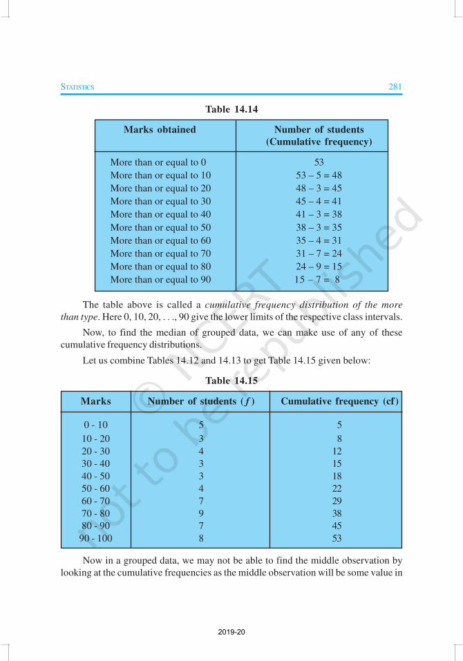
STATISTICS 281

Table 14.14


(Cumulative frequency)

More than or equal to 0 53

More than or equal to 10 53 – 5 = 48









The table above is called a cumulative frequency distribution of the more

than type. Here 0, 10, 20, . . ., 90 give the lower limits of the respective class intervals.

Now, to find the median of grouped data, we can make use of any of these

cumulative frequency distributions.

Let us combine Tables 14.12 and 14.13 to get Table 14.15 given below:

Table 14.15

Marks Number of students ( f ) Cumulative frequency (cf)

0 - 10 5 5

10 - 20 3 8

20 - 30 4 12

30 - 40 3 15

40 - 50 3 18

50 - 60 4 22

60 - 70 7 29

70 - 80 9 38

80 - 90 7 45

90 - 100 8 53

Now in a grouped data, we may not be able to find the middle observation by

looking at the cumulative frequencies as the middle observation will be some value in

2019-20

282 MATHEMATICS

a class interval. It is, therefore, necessary to find the value inside a class that divides

the whole distribution into two halves. But which class should this be?

To find this class, we find the cumulative frequencies of all the classes and 2

n.

We now locate the class whose cumulative frequency is greater than (and nearest to)

2

n⋅ This is called the median class. In the distribution above, n = 53. So,

2

n = 26.5.

Now 60 – 70 is the class whose cumulative frequency 29 is greater than (and nearest

to) 2

n, i.e., 26.5.

Therefore, 60 – 70 is the median class.

After finding the median class, we use the following formula for calculating the

median.

Median =cf

2+ ,

n

l hf

−

×

where l = lower limit of median class,

n = number of observations,

cf = cumulative frequency of class preceding the median class,

f = frequency of median class,

h = class size (assuming class size to be equal).

Substituting the values 26.5,2

n= l = 60, cf = 22, f = 7, h = 10

in the formula above, we get

Median =26.5 22

60 107

− + ×

= 60 + 45

7

= 66.4

So, about half the students have scored marks less than 66.4, and the other half have

scored marks more than 66.4.

2019-20

STATISTICS 283

Example 7 : A survey regarding the heights (in cm) of 51 girls of Class X of a school

was conducted and the following data was obtained:

Height (in cm) Number of girls

Less than 140 4

Less than 145 11

Less than 150 29

Less than 155 40

Less than 160 46

Less than 165 51

Find the median height.

Solution : To calculate the median height, we need to find the class intervals and their

corresponding frequencies.

The given distribution being of the less than type, 140, 145, 150, . . ., 165 give the

upper limits of the corresponding class intervals. So, the classes should be below 140,

140 - 145, 145 - 150, . . ., 160 - 165. Observe that from the given distribution, we find

that there are 4 girls with height less than 140, i.e., the frequency of class interval

below 140 is 4. Now, there are 11 girls with heights less than 145 and 4 girls with

height less than 140. Therefore, the number of girls with height in the interval

140 - 145 is 11 – 4 = 7. Similarly, the frequency of 145 - 150 is 29 – 11 = 18, for

150 - 155, it is 40 – 29 = 11, and so on. So, our frequency distribution table with the

given cumulative frequencies becomes:

Table 14.16

Class intervals Frequency Cumulative frequency

Below 140 4 4

140 - 145 7 11

145 - 150 18 29

150 - 155 11 40

155 - 160 6 46

160 - 165 5 51

2019-20

284 MATHEMATICS

Now n = 51. So, 51

25.52 2

n= = . This observation lies in the class 145 - 150. Then,

l (the lower limit) = 145,

cf (the cumulative frequency of the class preceding 145 - 150) = 11,

f (the frequency of the median class 145 - 150) = 18,

h (the class size) = 5.

Using the formula, Median = l +

cf2

n

hf

−

×

, we have

Median =25.5 11

145 518

− + ×

= 145 + 72.5

18 = 149.03.

So, the median height of the girls is 149.03 cm.

This means that the height of about 50% of the girls is less than this height, and

50% are taller than this height.

Example 8 : The median of the following data is 525. Find the values of x and y, if the

total frequency is 100.

Class interval Frequency

0 - 100 2

100 - 200 5

200 - 300 x

300 - 400 12

400 - 500 17

500 - 600 20

600 - 700 y

700 - 800 9

800 - 900 7

900 - 1000 4

2019-20

STATISTICS 285

Solution :

Class intervals Frequency Cumulative frequency

0 - 100 2 2

100 - 200 5 7

200 - 300 x 7 + x

300 - 400 12 19 + x

400 - 500 17 36 + x

500 - 600 20 56 + x

600 - 700 y 56 + x + y

700 - 800 9 65 + x + y

800 - 900 7 72 + x + y

900 - 1000 4 76 + x + y

It is given that n = 100

So, 76 + x + y = 100, i.e., x + y = 24 (1)

The median is 525, which lies in the class 500 – 600

So, l = 500, f = 20, cf = 36 + x, h = 100

Using the formula : Median =

cf2 ,

n

l hf

−

+

we get

525 =50 36

500 10020

x− − + ×

i.e., 525 – 500 = (14 – x) × 5

i.e., 25 = 70 – 5x

i.e., 5x = 70 – 25 = 45

So, x = 9

Therefore, from (1), we get 9 + y = 24

i.e., y = 15

2019-20

286 MATHEMATICS

Now, that you have studied about all the three measures of central tendency, let

us discuss which measure would be best suited for a particular requirement.

The mean is the most frequently used measure of central tendency because it

takes into account all the observations, and lies between the extremes, i.e., the largest

and the smallest observations of the entire data. It also enables us to compare two or

more distributions. For example, by comparing the average (mean) results of students

of different schools of a particular examination, we can conclude which school has a

better performance.

However, extreme values in the data affect the mean. For example, the mean of

classes having frequencies more or less the same is a good representative of the data.

But, if one class has frequency, say 2, and the five others have frequency 20, 25, 20,

21, 18, then the mean will certainly not reflect the way the data behaves. So, in such

cases, the mean is not a good representative of the data.

In problems where individual observations are not important, and we wish to find

out a ‘typical’ observation, the median is more appropriate, e.g., finding the typical

productivity rate of workers, average wage in a country, etc. These are situations

where extreme values may be there. So, rather than the mean, we take the median as

a better measure of central tendency.

In situations which require establishing the most frequent value or most popular

item, the mode is the best choice, e.g., to find the most popular T.V. programme being

watched, the consumer item in greatest demand, the colour of the vehicle used by

most of the people, etc.

Remarks :

1. There is a empirical relationship between the three measures of central tendency :

3 Median = Mode + 2 Mean

2. The median of grouped data with unequal class sizes can also be calculated. However,

we shall not discuss it here.

2019-20

STATISTICS 287

EXERCISE 14.3

1. The following frequency distribution gives the monthly consumption of electricity of

68 consumers of a locality. Find the median, mean and mode of the data and compare

them.

Monthly consumption (in units) Number of consumers

65 - 85 4

85 - 105 5

105 - 125 13

125 - 145 20

145 - 165 14

165 - 185 8

185 - 205 4

2. If the median of the distribution given below is 28.5, find the values of x and y.

Class interval Frequency

0 - 10 5

10 - 20 x

20 - 30 20

30 - 40 15

40 - 50 y

50 - 60 5

Total 60

3. A life insurance agent found the following data for distribution of ages of 100 policy

holders. Calculate the median age, if policies are given only to persons having age 18

years onwards but less than 60 year.

2019-20

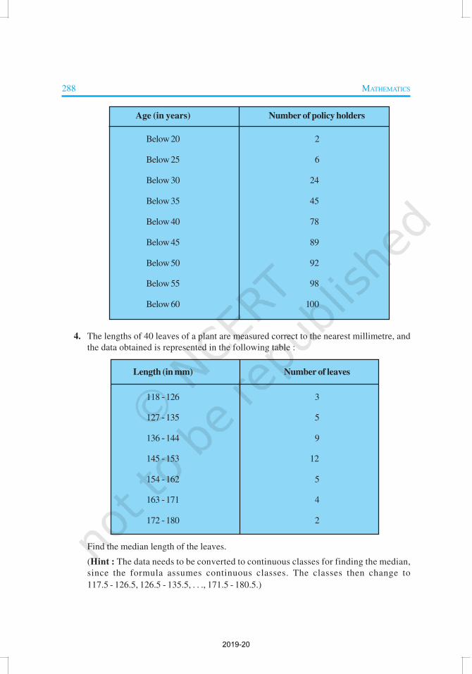
288 MATHEMATICS

Age (in years) Number of policy holders

Below 20 2

Below 25 6

Below 30 24

Below 35 45

Below 40 78

Below 45 89

Below 50 92

Below 55 98

Below 60 100

4. The lengths of 40 leaves of a plant are measured correct to the nearest millimetre, and

the data obtained is represented in the following table :

Length (in mm) Number of leaves

118 - 126 3

127 - 135 5

136 - 144 9

145 - 153 12

154 - 162 5

163 - 171 4

172 - 180 2

Find the median length of the leaves.

(Hint : The data needs to be converted to continuous classes for finding the median,

since the formula assumes continuous classes. The classes then change to

117.5 - 126.5, 126.5 - 135.5, . . ., 171.5 - 180.5.)

2019-20

STATISTICS 289

5. The following table gives the distribution of the life time of 400 neon lamps :

Life time (in hours) Number of lamps

1500 - 2000 14

2000 - 2500 56

2500 - 3000 60

3000 - 3500 86

3500 - 4000 74

4000 - 4500 62

4500 - 5000 48

Find the median life time of a lamp.

6. 100 surnames were randomly picked up from a local telephone directory and the

frequency distribution of the number of letters in the English alphabets in the surnames

was obtained as follows:

Number of letters 1 - 4 4 - 7 7 - 10 10 - 13 13 - 16 16 - 19

Number of surnames 6 30 40 16 4 4

Determine the median number of letters in the surnames. Find the mean number of

letters in the surnames? Also, find the modal size of the surnames.

7. The distribution below gives the weights of 30 students of a class. Find the median

weight of the students.

Weight (in kg) 40 - 45 45 - 50 50 - 55 55 - 60 60 - 65 65 - 70 70 - 75

Number of students 2 3 8 6 6 3 2

14.5 Graphical Representation of Cumulative Frequency Distribution

As we all know, pictures speak better than words. A graphical representation helps us

in understanding given data at a glance. In Class IX, we have represented the data

through bar graphs, histograms and frequency polygons. Let us now represent a

cumulative frequency distribution graphically.

For example, let us consider the cumulative frequency distribution given in

Table 14.13.

2019-20

290 MATHEMATICS

Recall that the values 10, 20, 30,

. . ., 100 are the upper limits of the

respective class intervals. To represent

the data in the table graphically, we mark

the upper limits of the class intervals on

the horizontal axis (x-axis) and their

corresponding cumulative frequencies

on the vertical axis ( y-axis), choosing a

convenient scale. The scale may not be

the same on both the axis. Let us now

plot the points corresponding to the

ordered pairs given by (upper limit,

corresponding cumulative frequency),

i.e., (10, 5), (20, 8), (30, 12), (40, 15),

(50, 18), (60, 22), (70, 29), (80, 38), (90, 45), (100, 53) on a graph paper and join them

by a free hand smooth curve. The curve we get is called a cumulative frequency

curve, or an ogive (of the less than type). (See Fig. 14.1)

The term ‘ogive’ is pronounced as ‘ojeev’ and is derived from the word ogee.

An ogee is a shape consisting of a concave arc flowing into a convex arc, so

forming an S-shaped curve with vertical ends. In architecture, the ogee shape

is one of the characteristics of the 14th and 15th century Gothic styles.

Next, again we consider the cumulative frequency distribution given in

Table 14.14 and draw its ogive (of the more than type).

Recall that, here 0, 10, 20, . . ., 90

are the lower limits of the respective class

intervals 0 - 10, 10 - 20, . . ., 90 - 100. To

represent ‘the more than type’ graphically,

we plot the lower limits on the x-axis and

the corresponding cumulative frequencies

on the y-axis. Then we plot the points

(lower limit, corresponding cumulative

frequency), i.e., (0, 53), (10, 48), (20, 45),

(30, 41), (40, 38), (50, 35), (60, 31),

(70, 24), (80, 15), (90, 8), on a graph paper,

and join them by a free hand smooth curve.

The curve we get is a cumulative frequency curve, or an ogive (of the more than

type). (See Fig. 14.2)

Fig. 14.1

Fig. 14.2

2019-20

STATISTICS 291

Fig. 14.3

Fig. 14.4

Remark : Note that both the ogives (in Fig. 14.1 and Fig. 14.2) correspond to the

same data, which is given in Table 14.12.

Now, are the ogives related to the median in any way? Is it possible to obtain the

median from these two cumulative frequency curves corresponding to the data in

Table 14.12? Let us see.

One obvious way is to locate

5326.5

2 2

n= = on the y-axis (see Fig.

14.3). From this point, draw a line parallel

to the x-axis cutting the curve at a point.

From this point, draw a perpendicular to

the x-axis. The point of intersection of

this perpendicular with the x-axis

determines the median of the data (see

Fig. 14.3).

Another way of obtaining the

median is the following :

Draw both ogives (i.e., of the less

than type and of the more than type) on

the same axis. The two ogives will

intersect each other at a point. From this

point, if we draw a perpendicular on the

x-axis, the point at which it cuts the

x-axis gives us the median (see Fig. 14.4).

Example 9 : The annual profits earned by 30 shops of a shopping complex in a

locality give rise to the following distribution :

Profit (Rs in lakhs) Number of shops (frequency)








2019-20

292 MATHEMATICS

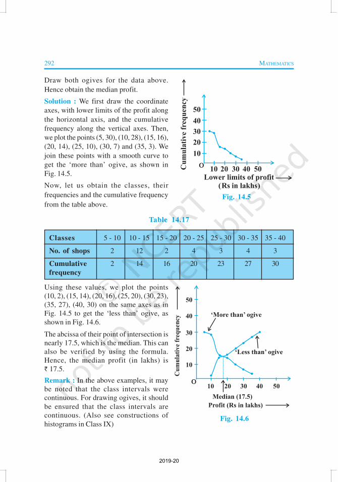
Draw both ogives for the data above.

Hence obtain the median profit.

Solution : We first draw the coordinate

axes, with lower limits of the profit along

the horizontal axis, and the cumulative

frequency along the vertical axes. Then,

we plot the points (5, 30), (10, 28), (15, 16),

(20, 14), (25, 10), (30, 7) and (35, 3). We

join these points with a smooth curve to

get the ‘more than’ ogive, as shown in

Fig. 14.5.

Now, let us obtain the classes, their

frequencies and the cumulative frequency

from the table above.

Table 14.17

Classes 5 - 10 10 - 15 15 - 20 20 - 25 25 - 30 30 - 35 35 - 40

No. of shops 2 12 2 4 3 4 3

Cumulative 2 14 16 20 23 27 30

frequency

Using these values, we plot the points

(10, 2), (15, 14), (20, 16), (25, 20), (30, 23),

(35, 27), (40, 30) on the same axes as in

Fig. 14.5 to get the ‘less than’ ogive, as

shown in Fig. 14.6.

The abcissa of their point of intersection is

nearly 17.5, which is the median. This can

also be verified by using the formula.

Hence, the median profit (in lakhs) is

` 17.5.

Remark : In the above examples, it may

be noted that the class intervals were

continuous. For drawing ogives, it should

be ensured that the class intervals are

continuous. (Also see constructions of

histograms in Class IX)

Fig. 14.5

Fig. 14.6

2019-20

STATISTICS 293

EXERCISE 14.4

1. The following distribution gives the daily income of 50 workers of a factory.

Daily income (in ̀ ) 100 - 120 120 - 140 140 - 160 160 - 180 180 - 200

Number of workers 12 14 8 6 10

Convert the distribution above to a less than type cumulative frequency distribution,

and draw its ogive.

2. During the medical check-up of 35 students of a class, their weights were recorded as

follows:

Weight (in kg) Number of students

Less than 38 0

Less than 40 3

Less than 42 5

Less than 44 9

Less than 46 14

Less than 48 28

Less than 50 32

Less than 52 35

Draw a less than type ogive for the given data. Hence obtain the median weight from

the graph and verify the result by using the formula.

3. The following table gives production yield per hectare of wheat of 100 farms of a village.

Production yield 50 - 55 55 - 60 60 - 65 65 - 70 70 - 75 75 - 80

(in kg/ha)

Number of farms 2 8 12 24 38 16

Change the distribution to a more than type distribution, and draw its ogive.

14.6 Summary

In this chapter, you have studied the following points:

1. The mean for grouped data can be found by :

(i) the direct method : i i

i

f xx

f

Σ=

Σ

2019-20

294 MATHEMATICS

(ii) the assumed mean method : i i

i

f dx a

f

Σ= +

Σ

(iii) the step deviation method : i i

i

f ux a h

f

Σ= + ×

Σ ,

with the assumption that the frequency of a class is centred at its mid-point, called its

class mark.

2. The mode for grouped data can be found by using the formula:

Mode = 1 0

1 0 22

f fl h

f f f

−+ ×

− − where symbols have their usual meanings.

3. The cumulative frequency of a class is the frequency obtained by adding the frequencies

of all the classes preceding the given class.

4. The median for grouped data is formed by using the formula:

Median =

cf2

n

l hf

−

+ ×

,

where symbols have their usual meanings.

5. Representing a cumulative frequency distribution graphically as a cumulative frequency

curve, or an ogive of the less than type and of the more than type.

6. The median of grouped data can be obtained graphically as the x-coordinate of the point

of intersection of the two ogives for this data.

A NOTE TO THE READER

For calculating mode and median for grouped data, it should be

ensured that the class intervals are continuous before applying the

formulae. Same condition also apply for construction of an ogive.

Further, in case of ogives, the scale may not be the same on both the axes.

2019-20

chap-14 (14th nov.) · solution: recall that to find the mean marks, we require the product of each...

Documents