channel estimation and code word inference for mobile digital
TRANSCRIPT


Channel Estimation and Code Word Inference for Mobile Digital
Satellite Broadcasting Reception
Masatoshi HamadaThe Japan Broadcasting Corporation (NHK)
Shiro IkedaThe Institute of Statistical Mathematics
October 28, 2008
Abstract
This paper proposes a method of improving reception of digital satellite broadcasting in a moving
vehicle. According to some studies, the antennas used for mobile reception will be smaller in the next
generation and reception will be more difficult because of a fading multipath channel with delays
in a low carrier-to-noise ratio. Commonly used approaches to reduce the inter symbol interference
caused by a fading multipath channel with delays are pilot sequences and diversity reception. Digital
satellite broadcasting, however, does not transmit pilot sequences for channel estimation and it is
not possible to install multiple antennas in a vehicle. This paper does not propose any change to
the broadcasting standards but discusses how to process currently available digital satellite signals
to obtain better results. Our method does not rely on the pilot sequences or diversity reception,
but consists of channel estimation and stochastic inference methods. For each task, two methods are
proposed. The maximum likelihood estimation and higher order statistics matching methods are pro-
posed for the estimation, and the marginal with the joint probability inference methods are proposed
for the stochastic inference. The improvements were confirmed through experiments with numerical
simulations and real data. The computational costs are also discussed for future implementation.
1 Introduction
Since the 1990s, it has become popular to install television reception systems in vehicles and more peopleare viewing television programs in the mobile environment [13].
Mobile reception is generally difficult. Among the many causes of the difficulties, we discuss two: theDoppler shift and the fading multipath channel. The influence of the Doppler shift can be removed withthe phase locked loop (PLL). When a fast PLL is used, the influence of the Doppler shift is negligible.
Commonly used approaches to reducing the influence of fading are the pilot sequence and diversityreception [3]. If the code includes a predetermined pilot sequence, the fading channel can be estimated.However, the current digital satellite broadcasting has only a one-byte known sequence, which is notenough for channel estimation. On the other hand, it is not possible to install multiple satellite anten-nas for diversity reception in vehicles, either. These are the reasons mobile reception of the satellitebroadcasting more difficult than that of terrestrial broadcasting.
STRADA (Panasonic) is one of the commercial mobile reception products for the digital satellitebroadcasting. It recommends that users should install an automatic machine tracking parabolic antennato enhance the direct reception and reduce the reflected paths. Although this effectively reduces theinfluence of the fading, the antenna is rather large and expensive. Some studies of next-generation mobilereception of the digital satellite broadcasting have indicated that smaller antennas are preferable [16].The carrier-to-noise (CNR) of such a compact antenna will be much lower than that for the standardparabolic antenna for static reception of digital satellite broadcasting [16]. What is worse is that thedirectivity is poor and it is not possible to eliminate the reflected waves that cause a fading multipathchannel with delays[16].
1

What we propose in this paper is not a new standard for digital satellite broadcasting. No pilotsequence is assumed, and the carrier frequency is not changed. Our proposal is to enhance the receivedsignals that are currently available from the satellite while still using an antenna with poor directivityand low CNR. Our method consists of channel estimation and stochastic inference of the codes.
Blind channel estimation is a popular idea [9] and we discuss two estimation methods for it. One is thecommonly used maximum likelihood estimation (MLE) and the other is the higher order statistics (HOS)matching method. For MLE, we need to utilize the expectation maximization (EM) algorithm [4]. TheEM algorithm is an iterative algorithm and its computational cost is relatively high. The HOS matchingmethod may not be as stable as MLE, but its computational cost is very low.
For the stochastic inference, we propose two methods. One is to utilize the marginal distributionof the fading channel model and the other is to utilize the joint distribution. The idea is equivalent toinference based on the graphical model [8], which is commonly used [19, 18, 11]. Our proposal is to findthe trade-off between the computational cost and the improvement.
The combinations of the proposed estimation and the stochastic inference methods were verified withsimulated data and measured real channel data of the digital satellite broadcasting. The results show thatour method improved the reception. The computational cost is reasonable enough for implementation.
Although the blind channel estimation and the stochastic inference are shown in some former studies [9,19, 18, 11], this paper newly shows two items. One is the practical channel model for the mobile digitalsatellite broadcasting reception. The reference [16] gives suggestions about a multipath channel in Ku-band land mobile satellite broadcasting. The multipath of twelve symbol time delay is considered in thereference. We consider the direct path and one symbol delay path for the channel model and deal themultipath of more than one symbol time delay as the noise. Our consideration gives a simple model whichis enough for the practical use. The other is the specific computational expression of the HOS under thechannel model. Although an idea of the HOS is shown in the reference [9], the specific computationalexpression is not explained. We show the constrained conditions to obtain the unique solution under thechannel model.
This paper is organized as follows. Section 2 describes the digital satellite broadcasting system andthe problem of mobile reception. Section 3 outlines the proposed method. Section 4 gives details ofthe channel description and two channel estimation methods. Section 5 shows two approaches for codeinference. Section 6 presents experimental results for the numerical simulation and real mobile reception.Finally, section 7 concludes the paper with a summary and some discussion.
2 Digital Satellite Broadcasting
2.1 Encoding and Modulation
First, we describe the encoding and modulation processes of digital satellite broadcasting. In this paper,we focus on two standards for digital satellite broadcasting (ARIB STD-B20 and DVB-S), which are thestandards for NHK BS digital.
Figure 1: Encoding and Modulation.
The encoding and modulation processes are schematically shown in Fig. 1. First, information bitsare encoded with the Reed-Solomon (RS) code [6] and the convolutional code. The RS code is based onGalois field GF(28), whose element is 1 byte = 8 bits. The RS(204, 188) code is used, where each 188bytes is encoded into 204 bytes. Basically, errors of 8 bytes can be corrected with this RS code. Oneblock of RS(204, 188) is 204 bytes = 8×204 = 1632 bits. The outputs of the RS code are interleaved andconcatenated with a convolutional code, whose constraint length is 7. The code rate of the convolutionalcode is 7/8. Finally, the output of the convolutional code is modulated with quadrature phase shiftkeying (QPSK). In this paper, we focus on the channel properties and the convolutional code and do notdiscuss the RS code in detail.
2

Let u = (u0, u1, · · · , um−1) ∈ {1, 0}m be the interleaved output of the RS code, where m > 7. Let us
define the i-th output of the convolutional code as xi = (xIi , x
Qi ) ∈ {−1,+1}2, which is defined as follows:
xIi = 1 − 2 (ui + ui−1 + ui−2 + ui−3 + ui−6)
xQi = 1 − 2 (ui + ui−2 + ui−3 + ui−5 + ui−6).
(1)
Neglecting the further puncturing process, we define eq. (1) as the encoding of the convolutional code.
Finally, xIi ∈ {−1,+1} and xQ
i ∈ {−1,+1} are modulated by QPSK defined as
FQPSK(t) = b[
xIi cos(2πfct) + xQ
i sin(2πfct)]
, iTs ≤ t < (i+ 1)Ts, (2)
where Ts is the duration of each bit (43.0404 ns), fc is the carrier frequency, and b denotes the amplitude.In the case of NHK BS digital, fs ≡ 1/Ts, which we call the “symbol rate” is 23.234 MHz, fc is around12 GHz, and fc is divisible by fs.
2.2 Static Reception
Digital satellite broadcasting is generally received fairly well from a fixed place with a BS/CS (broad-casting satellite and communication satellite) receiving dish antenna having a rather large bore diameter(40 to 50 cm). The received CNR range of static reception is very high (more than 14 dB) because ofthe parabolic antenna. A conventional method of demodulation and decoding is shown in Figure 2. The
Figure 2: Conventional Demodulation and Decoding.
coherent QPSK demodulation is defined as the time average of the products of cos(2πfct) or sin(2πfct)
and the received signal FQPSK(t). Let us define yi = (yIi , y
Qi )T as follows:
yIi = B
∫ (i+1)Ts
iTs
FQPSK(t) cos(2πfct)dt, yQi = B
∫ (i+1)Ts
iTs
FQPSK(t) sin(2πfct)dt, (3)
where B is a factor for making yIi2
+ yQi
2= 2. Each component of yi is not binary in practice because
of the noise. However, in the case of static reception, the difference between yi and xi is small. In thefollowing, we define x as the sequence of xq, · · · , xq+N . In a similar manner, y and u show the sequence.The basic idea for decoding y to uH [15] is summarized in the following equation:
uH = argminu
dH(sign(y),x(u)), (4)
where dH(·, ·) is the Hamming distance, x(u) is the function defined in eq. (1), and argminu defines theu that minimizes the quantity. In eq. (4), the u that minimizes the total Hamming distance is selected.In the following, we denote the decoded result of y as uH . Some errors in uH are corrected by the RSdecoding, and the final error rate is very low in static reception.
Since the reception antennas for static reception are large enough to focus only on the direct path,it is possible to assume that the channel is stationary and memoryless. Under this assumption, thereceived information about each bit can be regarded as an independent observation, and the decodingwith Hamming distance works well.
2.3 Mobile Reception
Compared with static reception, mobile reception of digital satellite broadcasting is difficult. We can seethis from the fact that there are very few commercial products for mobile reception.
The difficulty arises from two main reasons: the Doppler shift and the fading multipath channel [15].We explain these first.
3

In the mobile reception, the relative velocity between the satellite and the vehicle is not 0, so itproduces a Doppler shift. If a vehicle moves at 100 km/h toward the satellite, the Doppler shift is around1 kHz because the carrier frequency is 12 GHz. This is much smaller than the symbol rate, which isfs = 23 MHz, but the Doppler shift influences the QPSK demodulation. One of the general approachesto reducing the influence of the Doppler shift is to use a phase locked loop (PLL).
In the case of static reception, dish antennas are used. Since they have narrow directivities, theinfluence of the multipath channel can be neglected. However, in mobile reception, antennas are generallysmall because they must be installed in a vehicle and their directivities are poor. We assume that thedirect path between the satellite and the vehicle is not occluded, but that the influence of the multipathchannel is not negligible. Moreover, it is natural to assume that the characteristics of the channel changeas the vehicle moves.
Next, let us discuss how these problems are solved in commercial products. Among the few commercialdigital satellite broadcasting receivers for vehicles, STRADA (Panasonic) is the one with a reasonableprice. Although details of the receiver are not available, it seems (from personal communication) thesystem uses a fast PLL. A PLL resets the influence of the Doppler shift at every acquisition time and ifthe PLL is fast enough, the influence of the Doppler shift can be neglected.
To reduce the influence of the fading channel, Panasonic recommends that customers should use anantenna with a tracking system that has narrow directivity, which makes the main path is dominant andreflections small.
The strategy of using a PLL and an antenna with a tracking system for the Doppler shift and fadingmultipath channel, respectively, is effective.
3 Proposed Method
3.1 Our Strategy
The ultimate goal of our research is to make a compact receiving system with a reasonable price. We donot propose any change to the broadcasting standard. We receive the signal that is currently availablefrom the satellite and improve the quality of the received broadcasting.
Our strategy is different from the available commercial products. To reduce the influence of theDoppler shift, we also use a fast PLL, but we do not use a tracking antenna because an antenna with atracking system is rather large and expensive.
According to discussions of the ideal next-generation mobile reception antennas [16], a three-beamantenna that covers 360 degree (each beam is 120 degree) in azimuth angle has good characteristics [7].Antennas of this type are compact enough to be installed to vehicles. However, the CNR range of suchantennas will be relatively low [16]. Another study indicates that the next-generation antenna gain formobile reception will be around 25 dBi to 37 dBi [17]. What is worse is that since the directivities ofsuch antennas are poor, it is not possible to ignore the reflected waves even if the carrier frequency ishigh (over 10 GHz) and the channel becomes a fading multipath channel with delays [16, 13, 15].
One of the commonly used approaches for channels with memory is to install multiple antennas fordiversity reception. However, it is not possible to install multiple digital satellite broadcasting antennas ina vehicle. Another commonly used approach is to utilize pilot sequences. These enable the characteristicsof the fading channel to be estimated. However, the NHK digital satellite broadcasting has only one fixedword (8 bits) in each block of RS(204, 188), and this is not long enough as the pilot sequence.
The method that we propose does not rely on diversity reception or pilot sequences, but uses thestochastic channel model and recovers the information bits by using stochastic inference.
3.2 Channel Model and Stochastic Inference
The channel model is generally described as a stochastic model p(y|x(u)), which is the conditionalprobability of y when x(u) is given. When y is observed, a natural inference on u is to take u =argmaxu p(x(u)|y) by assuming that the prior distribution of x is uniform as p(x) = 1/22N (N is thelength of x) and using the Bayes theorem:
p(x(u)|y) =p(y|x(u))p(x)
∑
x p(y|x(u))p(x)∝ p(y|x(u)).
4

Therefore,
u = argmaxu
p(x(u)|y) = argmaxu
p(y|x(u)). (5)
Moreover, if the channel is a binary symmetric channel (BSC) with flipping probability α < 1/2, whichis a typical memoryless channel, then
p(y|x(u)) =∏
i
p(yi|xi(u)) =∏
i
αdH (yi,xi(u))(1 − α)2−dH (yi,xi(u)) ∝(1 − α
α
)
−dH(y,x(u))
.
Since α < 1/2, ((1 − α)/α) > 1, the maximization of p(y|x(u)) is equivalent to the minimization ofdH(y,x(u)) regardless of α. Therefore eq. (5) becomes equivalent to eq. (4).
When the channel has memory, the bits of y are not independent and eq. (4) does not work. We stilluse eq.(5), based on the stochastic channel model with memory. What we need to discuss below is howto build the channel model and how to utilize it to solve eq. (5).
In the case of a BSC, parameter α does not have any influence on the decoding algorithm, but inthe case of fading channels, the parameters must be estimated and used to solve eq. (5). The channelmodel and parameter estimation methods are discussed in detail in section 4. We use the stochasticmodel with adjacent inter symbol interference (ISI). We explain why we chose this model in section 4.The parameter estimation of the channel is not simple because the channel input sequence u is hiddenfrom the observed signal y. We discuss two methods [19, 9]: MLE and HOS matching. For MLE, we usethe EM algorithm[4]. Although the EM algorithm is simple, iterative computation is inevitable and thistakes time. The estimation based on HOS may not be as stable as that of MLE, but the computationalcost is very low, which is better for practical implementation. We compare them in section 6.
When y is observed, the channel model gives us p(x(u)|y). In section 5, we discuss two methods ofstochastic inference ([18, 11]) based on p(x(u)|y).
One is to use the marginal distribution p(xi(u)|y) and compute u based on it (marginal inference).The other is to use the joint probability of p(x(u)|y) to compute u (joint inference) (Fig. 3). In eachcase, the decoded codeword of u is further decoded by the RS decoder (Fig. 3). Since the computationalcost is slightly different, we compare the costs and results of the methods.
Figure 3: Schematic Diagram of the Proposed Method.
For the following discussion, we define variables x, u, and u as follows.
x : The stochastic inference of the hard bits based on the fading channel estimation.
u : The stochastic inference on u based on p(xi(u)|y).
u : The stochastic inference on u based on p(x(u)|y).
5
4 Fading Channel and Estimation
4.1 Model of Fading Channel
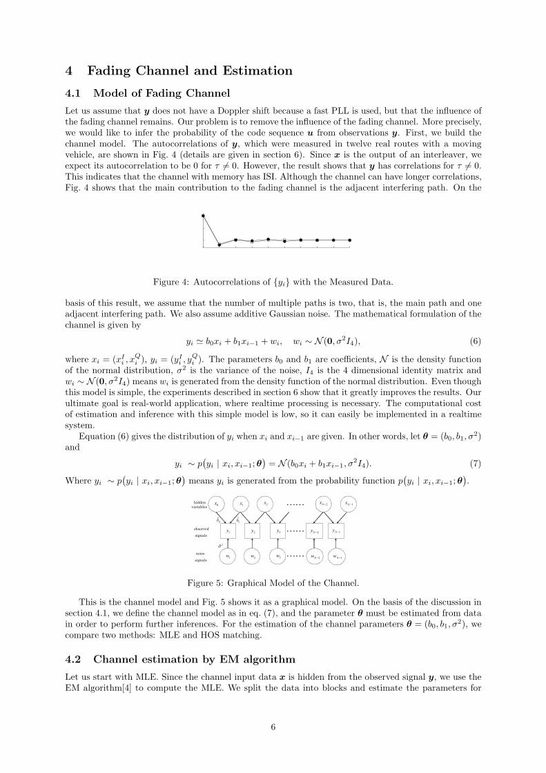
Let us assume that y does not have a Doppler shift because a fast PLL is used, but that the influence ofthe fading channel remains. Our problem is to remove the influence of the fading channel. More precisely,we would like to infer the probability of the code sequence u from observations y. First, we build thechannel model. The autocorrelations of y, which were measured in twelve real routes with a movingvehicle, are shown in Fig. 4 (details are given in section 6). Since x is the output of an interleaver, weexpect its autocorrelation to be 0 for τ 6= 0. However, the result shows that y has correlations for τ 6= 0.This indicates that the channel with memory has ISI. Although the channel can have longer correlations,Fig. 4 shows that the main contribution to the fading channel is the adjacent interfering path. On the
0 1 2 3 4 5 6 7 8 9
0
0.5
1
Ts [Ts=43.0404 nsec]
Aut
ocor
rela
tion
Figure 4: Autocorrelations of {yi} with the Measured Data.
basis of this result, we assume that the number of multiple paths is two, that is, the main path and oneadjacent interfering path. We also assume additive Gaussian noise. The mathematical formulation of thechannel is given by
yi ≃ b0xi + b1xi−1 + wi, wi ∼ N (0, σ2I4), (6)
where xi = (xIi , x
Qi ), yi = (yI
i , yQi ). The parameters b0 and b1 are coefficients, N is the density function
of the normal distribution, σ2 is the variance of the noise, I4 is the 4 dimensional identity matrix andwi ∼ N (0, σ2I4) means wi is generated from the density function of the normal distribution. Even thoughthis model is simple, the experiments described in section 6 show that it greatly improves the results. Ourultimate goal is real-world application, where realtime processing is necessary. The computational costof estimation and inference with this simple model is low, so it can easily be implemented in a realtimesystem.
Equation (6) gives the distribution of yi when xi and xi−1 are given. In other words, let θ = (b0, b1, σ2)
and
yi ∼ p(
yi | xi, xi−1; θ)
= N (b0xi + b1xi−1, σ2I4). (7)
Where yi ∼ p(
yi | xi, xi−1; θ)
means yi is generated from the probability function p(
yi | xi, xi−1; θ)
.
Figure 5: Graphical Model of the Channel.
This is the channel model and Fig. 5 shows it as a graphical model. On the basis of the discussion insection 4.1, we define the channel model as in eq. (7), and the parameter θ must be estimated from datain order to perform further inferences. For the estimation of the channel parameters θ = (b0, b1, σ
2), wecompare two methods: MLE and HOS matching.
4.2 Channel estimation by EM algorithm
Let us start with MLE. Since the channel input data x is hidden from the observed signal y, we use theEM algorithm[4] to compute the MLE. We split the data into blocks and estimate the parameters for
6

each block. The block length is set to N = 2000. Let block y = {y1, · · · , yN}. For the estimation, weuse MLE, which is defined as
θ = argmaxθ
p(y; θ) = argmaxθ
log p(y; θ).
The likelihood p(y; θ) is rewritten as
p(y; θ) =∑
x
p(y,x; θ) =∑
x
p(y|x; θ)p(x).
From eq. (7), p(y|x; θ) is easily rewritten as
p(y|x; θ) =
N∏
i=1
p(
yi | xi, xi−1; θ)
,
and the natural choice of p(x), which is the prior of x, is a uniform distribution p(x) = 1/22(N+1). Nowthe distributions p(y,x; θ) and p(y; θ) become
p(y,x; θ) =1
22(N+1)
N∏
i=1
p(
yi | xi, xi−1; θ)
(8)
p(y; θ) =1
22(N+1)
∑
x
N∏
i=1
p(
yi | xi, xi−1; θ)
. (9)
This is a mixture of normal distributions, and x is the hidden stochastic variable. In this situation, onewidely used method for MLE is the EM algorithm. We use the EM algorithm to compute the MLEof θ = (b0, b1, σ
2). The EM algorithm is a simple iterative method that consists of E- and M-steps formaximizing the log-likelihood function [4]. The algorithm is as follows.
E-step In the r-th round of the E-step, a Q function, which is defined below, is computed.
Q(θ,θr) =1
N
∑
x
p(x|y; θr) log p(y,x; θ)
From eqs. (7) and (8), Q(θ,θr) is rewritten as
Q(θ,θr) = − 1
N
∑
x
p(x|y; θr)
∣
∣yi − (b1xi−1 + b0xi)∣
∣
2
2σ2− log 2πσ2
= − 1
N
N∑
i=1
y2i
2σ2− b21 + b20
σ2− log 2πσ2 +
2b1σ2
Cryx
−1+
2b0σ2
Cryx − 2b0b1
σ2Cr
xx−1,
(10)
where the fact |xi|2 = 2 is used and Cryx
−1, Cr
yx, and Crxx
−1are defined as follows:
Cryx
−1=
1
2N
N∑
i=1
∑
xi−1
p(x|y; θr)yi · xi−1, Cryx =
1
2N
N∑
i=1
∑
xi
p(x|y; θr)yi · xi
Crxx
−1=
1
2N
N∑
i=1
∑
xi−1,xi
p(x|y; θr)xi−1 · xi.
(11)
It is necessary to compute CryN x
−1, Cr
yN x−1
, and Crxx
−1at every iteration. For the computation,
we can utilize the belief propagation (BP) algorithm. Details are given in section A.
M-step At each iteration, the M-step updates θ as
θr+1 = argmaxθ
Q(θ,θr).
7

If we equate ∂Q(θ,θr)/∂θ|θ=θr+1 = 0, it becomes
br+10 =
Cryx − Cr
yx−1Cr
xx−1
1 − (Crxx
−1)2
, br+11 =
Cryx
−1− Cr
yxCrxx
−1
1 − (Crxx
−1)2
σr+12=
1
2N
N∑
i=1
∣
∣yi
∣
∣
2+ br+1
1
2+ br+1
0
2 − 2br+11 Cr
yx−1
− 2br+10 Cr
yx + 2br+10 br+1
1 Crxx
−1.
At r = 0, θ0 is initialized as b00 = 0.8(2 − σ2), b01 = 0.2(2 − σ2) and σ2)0
= 0.3. In practice, the E-and M-steps are repeated and the algorithm with the initial condition converges well with a few to 20iterations. Finally, the parameter is estimated as θ = (b0, b1, σ
2).
4.3 Channel estimation by Higher Order Statistics
Next, we explain the HOS matching. From the model in eq. (6) and the assumptions that xi is indepen-dent, its mean is 0, and noise is independent additive Gaussian noise, we have the following relations:
Cyy = 2(b20 + b21 + σ2), Cyy−1
= 2b0b1,
Cy4 = 4{
(b20 + b21 + σ2)2 + 4σ2(b20 + b21 + σ2) − 2σ4 + 4b20b21
}
= 4{
2σ2Cyy +1
2C2
yy + C2yy
−1−σ4
} (12)
where we used the fact that Ep(z)[z4] = 3σ4 if z ∼ N (0, σ2) and the following quantity
Cyy = Ep(y)[yQi
2+ yI
i
2], Cy4 = Ep(y)[y
Qi
4+ yI
i
4], Cyy
−1= Ep(y)[y
Ii y
Ii−1 + yQ
i yQi−1].
In practice, we replace these with the following example means.
Cyy =1
N
∑
i
(
yQi
2+ yI
i
2)
, Cy4 =1
N
∑
i
(
yQi
4+ yI
i
4)
, Cyy−1
=1
N
∑
i
(yIi y
Ii−1 + yQ
i yQi−1).
The unknown parameters b0, b1, and σ2 can be estimated by solving the set of equations in eq. (12). It iseasy to check that the solutions are not unique from the fact that the equations in eq. (12) are symmetricfor b0 and b1.
Since b0 shows the signal strength from the direct path, we impose two constraints: b0 > 0 andb0 > |b1|.
σ2 = Cyy −√
3
2C2
yy + 2C2yy
−1− Cy4 ,
b0 =1√2
(
B2 +√
B2 − C2yy
−1
)1/2
, b1 =Cyy
−1
2b0, where B =
1
2Cyy − σ2.
This method strongly depends on the assumption that the noise is Gaussian, and the solution may not beas stable as that of MLE. However, the computation is straightforward and its cost is low. We comparethese two methods through experiments.
5 Inference of Convolutional Code
When the parameters of the channel are estimated with the MLE or HOS matching methods, the channelmodel p(y|x(u); θ) is given. We would like to make the stochastic inference on u, which is the inputs ofthe convolutional code, based on p(x(u)|y; θ).
In the following, we propose two approaches for stochastic inference. The first approach is to applystochastic inference to the hard bits of x and decode them by the conventional convolutional decoding. Wecall this approach the marginal inference approach. The other approach is to apply stochastic inferencedirectly to the input sequence of the convolutional encoding u. We show the graphical model of thetransmitting convolutional code words and the channel model. And the stochastic inference on theconvolutional code words is based on the graphical model. We call this method the joint inferenceapproach. Both approaches are discussed below.
8

5.1 Marginal Inference Approach
In the marginal inference approach, we first estimate x based on the marginal probability p(xi(u)|y).Let x be the inference of the sequence x. With an abuse of the notation, the inference x is defined asfollows:
xi = sign xi, xi =∑
xi
xip(xi|y; θ) (13)
This is the maximization of the posterior marginals; that is,
xi = argmaxxi
p(xi|y; θ).
The BP algorithm (A) is an efficient method for computing xi. To decode x to u, we use eq. (4):
u = argminu
dH(sign(x),x(u)). (14)
The standard decoding algorithm of convolutional codes solves this problem. We define u as the decodedword of this method.
5.2 Joint Inference Approach
In the joint inference approach, the stochastic inference on u is done based on p(x(u)|y; θ). The graphicalmodel representation is shown in Fig. 6, where code words u as well as x are the hidden stochasticvariables. We infer code u from the posterior distribution given observed signal y.
Figure 6: Graphical Model of Convolutional Code.
The idea of the inference is to find the path in the trellis that maximizes p(u|y; θ) as
u = argmaxu
p(u|y; θ) = argmaxu
∑
x
p(u|x)p(x|y; θ). (15)
From eq. (8), we have p(x|y; θ) as
p(x|y; θ) =p(x)p(y|x; θ)
∑
x p(x)p(y|x; θ)=
1
Z
N−1∏
i=1
p(yi|xi, xi−1; θ) =1
Z ′
N−1∏
i=1
ψt(xi, xi−1),
where
Z = 22N∑
x
p(y,x; θ), ψi(xi, xi−1) = exp
[
−∣
∣yi − (b0xi + b1xi−1)∣
∣
2
2σ2
]
Z ′ = (2πσ2)N−1Z =∑
x
N−1∏
i=1
ψi(xi, xi−1).
We use the BP algorithm[14] to compute p(x|y; θ) efficiently. In the following, we rewrite p(u|y; θ)as p(u) and denote uq
r for ur, · · · , uq, (q > r) for simplicity because the joint distribution p(uM−10 ) is
defined as
p(uM−10 ) = p(u6
0) p(u7|u60) · · · · · p(uM−1|uM−2
M−8)
log p(uM−10 ) = log p(u6
0) + log p(u7|u60) + · · · + log p(uM−1|uM−2
M−8).
9

The individual conditional probabilities are defined as
p(ui|ui−1i−7) =
p(uii−7)
p(ui−1i−7)
.
The trellis for the computation of u is shown in Fig. 7. Figure 7 starts from the initial status log p(u60)
and then moves to the next status log p(u7|u60). Final status is log p(uM−1|uM−2
M−8). The sequence uM−10
is searched for in the trellis as the path that maximizes p(uM−10 ).
Figure 7: Convolutional Code Inference.
6 Numerical Experiments
6.1 Simulated Data
We have proposed two channel estimation methods (MLE and HOS matching) and two stochastic infer-ence methods (marginal and joint inference). The combinations of each estimation and inference methodswere tested in two numerical experiments: one with simulated data and the other with real mobile channeldata.
First, we explain the experiment with simulated data. We generated data sets according to eq. (6).Each data set consists of 2000 data points, where b0 is fixed to 1.0, b1 is a sample taken from a uniformdistribution of [−1/K, 1/K], and the additive noise follows the Gaussian distribution as
wi ∼ N (0, σ2I4).
Note that b0 and b1 are fixed for each data set, and we repeated the experiments 100 times for each σ bydrawing b1 from a uniform distribution.
K = 10 K = 5 K = 1
Figure 8: Error Performances of the Outputs of Convolutional Code.
The error performances of the convolutional decoding are shown in Fig. 8. Each graph shows theresults for a different K. Each figure shows 7 results: combinations of the two channel estimationmethods and two inference methods, two inference methods with true parameters (since we know the
10

channel model parameters in the simulation), and standard decoding methods without the channel modelor joint inference (hard decision + Viterbi decoding).
As shown in Fig. 8, the method (MLE estimation or HOS matching) did not influence the results,but the joint inference worked better than the marginal inference. In each case, the results were close tothose obtained using the true parameters.
The maximum bit error rate (BER) to let RS decoding have an error ratio of less than 10−5 is typically2 × 10−3. Although wide rage of CNR is simulated in the refrence [16], we consider 8 dB to 10 dB ofCNR is the range of our experiments. This range is relatively low and the method shown in the reference[16] cannot improve the error performances enoughly. In this range, decoding without channel estimationcannot remove the influence of the fading channel. The marginal inference approach can improve theerror performances, but cannot achieve sufficient quality. The joint inference approach can remove theinfluence of the fading channel.
6.2 Measuring Real Channels on Twelve Routes
Next, we explain the experiment with the data for real channels of satellite broadcasting mobile reception.The measurement conditions are listed in Table 1.
Table 1: Measurement Conditions.Satellite BSAT-2a
Reception frequency 11.84256 GHzPlaces Tokyo and Kanagawa, Japan
Elevation angle 38.1 degreeAntenna gain 25 dBi
Date February 2, 2006Weather Fine
We used a multi-beam antenna [7] and a fast PLL whose acquisition time is equal to the symboltime. In our experiments, we installed a commercially produced Lunenburg lens antenna [7] (SumitomoElectric Industries, LuneQ-40 1) on the roof of a vehicle. The measuring system consisted of a low noiseamplifier module and an orthogonal signal recorder with a PLL whose acquisition time was one QPSKsymbol time.
The channel was measured on a fine day while the vehicle was moving along the K1-Yokohane highwayfrom Haneda toward Yokohama, the urban road around Ohta Ichiba in Shinagawa, and the city roadaround Aomonoyokocho in Shinagawa. The routes were chosen so as not to have any serious shadowing.We measured at five places along the highway (H1–H5), three places along the urban road (U1–U3), andfour places along the city road (C1–C4) (Fig. 9).
Highway Urban Road City Road
Figure 9: Measurement Routes (I.C.: interchange).
The autocorrelations for each route are shown in Fig. 10. The highway is an elevated expressway with
1Although this product is designed for static reception, the antenna was installed on a vehicle for the measurement.
11

few reflected waves. The urban road is surrounded by warehouses, and the city road is surrounded byoffice buildings, giving relatively many reflected waves and delays.
High Way Urban Road City Road
Figure 10: Examples of Autocorrelation.
In each route, the CNR was in the range of 8 to 10 dB. We recorded the frequency modulation (FM)signal broadcast from the satellite, where the original signal was known. The real channel was measuredat the sampling rate 92.936 MHz and the channel was reconstructed in the form of autocorrelations,where the data rate was 23.234 MHz. Data for 120 s was collected. We used data for twelve real channelin the experiments (Fig. 11). In this case, the original data was known and the error rates were computed.
Figure 11: Block Diagram of the Measurement.
6.3 Reconstruction of the Mobile Channel
For the experiments, the measured mobile channels had to be reconstructed from the measured FMsignals. An FM signal is generally expressed as
FFM (t) = a cos(2π(fc + fm(t))t),
where fm(t) is the frequency of the transmission signal, which we know.With the PLL, the mobile channel output signal of the FM signal, which is influenced by the Doppler
shift and the fading channel, can be expressed as
FFM (t) =
LF M−1∑
l=0
al cos(2π(fc + fm(t))(t − τl) +l(t)), l(t) = 2πfDl(t− τl) + φ0,
where al, τl, and l(t) are the amplitude, delay, and Doppler shift of the lth path, respectively. Sincewe know fm(t), the mobile channel characteristics are obtained by removing fm(t) from the recordedsignal. After that, the channel is approximated as a finite impulse response filter with 4096 taps, whichis defined as
hFM (t) ≡LF M−1
∑
l=0
al cos(
2π(fc + fDl)(t− τl) + φ0
)
=
4095∑
l=0
al cos(
2π(fc + fDl)(t− lTS) + φ0
)
.
Here, TS is given by the PLL. To get each multiple path amplitude and phase rotation, we multiplyhFM(t) by cos(2πfc(t− lTS)) and obtain the signal observed through the low pass filter as
bl cos(2πfDl(t− lTs) + φ0).
The Hilbert transformation gives us
bl sin(2πfDl(t− lTs) + φ0). (16)
12

In this way, the reproduced mobile channel is expressed as the filter. We can rewrite it as a filter fromxi to yi, which is expressed as a matrix defined as follows:
H(t) ≡4095∑
l=0
(
bl cosl(t) bl sinl(t)−bl sinl(t) bl cosl(t)
)
, l(t) = 2πfDl(t− lTs) + φ0.
The noise was also measured in the case of a different carrier, where no signal was sent. Letting the noisen(iTs), the received signal is reconstructed as
yi = H(iTs)xi + n(iTs).
6.4 Results
Here, we present the results obtained when our method was applied to the data for twelve mobile chan-nels. First, to explain how the multiple paths are removed, we show the autocorrelations of y and x,where y is the reception data and x is the inference based on the fading channel, as expressed by eq. (13).The original codes were interleaved and the ideal autocorrelations were 0 except for τ = 0. The autocor-relations for 3 out of 12 measured mobile channels (the results were similar for the other channels) areshown in Fig. 12. As y was processed to x, the autocorrelations got closer to the expected function.
Figure 12: Autocorrelations.
Next we show how the proposed method improves the results. We show the experimental schematicdiagrams in Fig.13. The results for u (the marginal inference approach) and u (the joint inference
Figure 13: Schematic Diagram of Experiments.
approach) are shown in Tables 2 and 3. For both inference approaches, two channel estimation methods(HOS matching and the EM algorithm) were combined. The BER of the outputs of the convolutionaldecoding and the element errors of the RS decoding are shown in Tables 2 and 3, respectively. Thesetables also show the results with uH (hard decision without channel estimation).
For NHK BS television reception, the quality of the received images was very good when the elementerror rate was less than 2 × 10⁻⁴ at the output of the RS decoding.
Comparing the marginal and joint inference approaches, the joint inference reached a good qualityrange in a practical CNR range (8 to 10 dB), while the marginal inference approach gave good resultsfor some routes (e.g., H1, H2, and U1), but performed badly for others (e.g., H5, U3, and C4).
Comparing the HOS matching and the EM algorithm, although there were almost no differences forthe numerical simulation, the EM algorithm worked slightly better than the HOS matching. The HOSmatching strongly relies on the noise being Gaussian that Ep(z)[z
4] = 3σ4 if z ∼ N (0, σ2), each x isindependent and the average of x is zero. This may indicate that the noise distribution of a real channelis non-Gaussian. However, at the output of the RS decoder, there were almost no differences.
We give a quantitative comment of the computational cost by measuring the execution time of MAT-LAB program. Comparing the decoding time expressed in Eq.(4), although the method combined theMLE estimation with Joint Inference times from 2.2 to 20.2, the method combined the HOS estimationwith Joint Inference times 1.3.
13

Table 2: BER of Convolutional Code.
Table 3: Element Error Rate of RS Code.
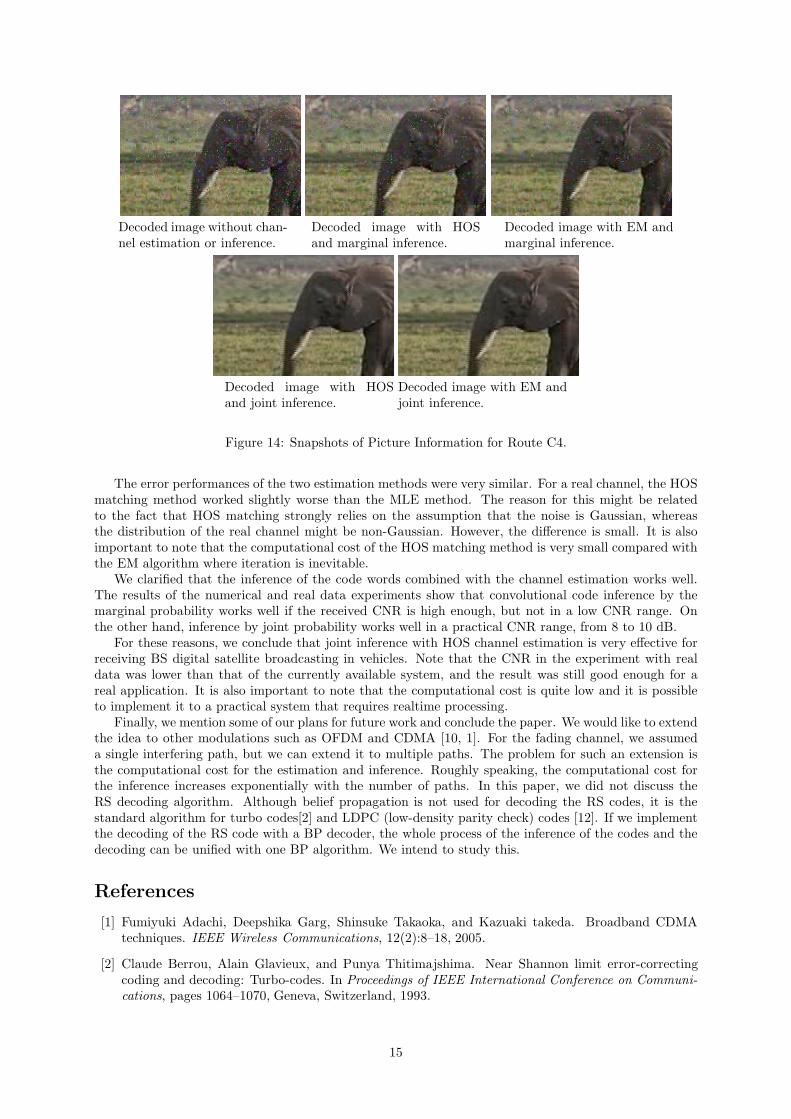
For further reference, we present pictures some results in Fig. 14. These are the snapshots of thedecoded images for route C4, whose received CNR was the lowest (around 8 dB). They show that thejoint inference approach with both HOS matching and the EM algorithm removed the influence of thereal digital satellite mobile channel.
Original picture. Enlarged original picture.
7 Conclusion
We proposed mobile reception methods to improve the quality of the received information in digitalsatellite broadcasting. These methods do not use any diversity reception or pilot sequences [5], but usechannel estimation and stochastic inference of code words based on a simple graphical model, whichrepresents the fading channel and the convolutional code. We proposed two channel estimation methodsand two stochastic inference methods. The estimation methods are MLE and HOS matching. Thestochastic inference methods are marginal inference and joint inference.
14
Decoded image without chan-nel estimation or inference.
Decoded image with HOSand marginal inference.
Decoded image with EM andmarginal inference.
Decoded image with HOSand joint inference.
Decoded image with EM andjoint inference.
Figure 14: Snapshots of Picture Information for Route C4.
The error performances of the two estimation methods were very similar. For a real channel, the HOSmatching method worked slightly worse than the MLE method. The reason for this might be relatedto the fact that HOS matching strongly relies on the assumption that the noise is Gaussian, whereasthe distribution of the real channel might be non-Gaussian. However, the difference is small. It is alsoimportant to note that the computational cost of the HOS matching method is very small compared withthe EM algorithm where iteration is inevitable.
We clarified that the inference of the code words combined with the channel estimation works well.The results of the numerical and real data experiments show that convolutional code inference by themarginal probability works well if the received CNR is high enough, but not in a low CNR range. Onthe other hand, inference by joint probability works well in a practical CNR range, from 8 to 10 dB.
For these reasons, we conclude that joint inference with HOS channel estimation is very effective forreceiving BS digital satellite broadcasting in vehicles. Note that the CNR in the experiment with realdata was lower than that of the currently available system, and the result was still good enough for areal application. It is also important to note that the computational cost is quite low and it is possibleto implement it to a practical system that requires realtime processing.
Finally, we mention some of our plans for future work and conclude the paper. We would like to extendthe idea to other modulations such as OFDM and CDMA [10, 1]. For the fading channel, we assumeda single interfering path, but we can extend it to multiple paths. The problem for such an extension isthe computational cost for the estimation and inference. Roughly speaking, the computational cost forthe inference increases exponentially with the number of paths. In this paper, we did not discuss theRS decoding algorithm. Although belief propagation is not used for decoding the RS codes, it is thestandard algorithm for turbo codes[2] and LDPC (low-density parity check) codes [12]. If we implementthe decoding of the RS code with a BP decoder, the whole process of the inference of the codes and thedecoding can be unified with one BP algorithm. We intend to study this.
References
[1] Fumiyuki Adachi, Deepshika Garg, Shinsuke Takaoka, and Kazuaki takeda. Broadband CDMAtechniques. IEEE Wireless Communications, 12(2):8–18, 2005.
[2] Claude Berrou, Alain Glavieux, and Punya Thitimajshima. Near Shannon limit error-correctingcoding and decoding: Turbo-codes. In Proceedings of IEEE International Conference on Communi-cations, pages 1064–1070, Geneva, Switzerland, 1993.
15

[3] James K. Cavers. An analysis of pilot symbol assisted modulation for Rayleigh fading channels.IEEE Transactions on Vehiclular Technology, 40(4):686–693, 1991.
[4] A. P. Dempster, N. M. Laird, and D. B. Rubin. Maximum likelihood from incomplete data via theEM algorithm. Journal of the Royal Statistical Society B, 39:1–38, 1977.
[5] Rrank A. Dietrich and Wolfgang Utschick. Maximum ratio combining of correlated Rayleigh fadingchannels with imperfect channel knowledge. IEEE Transactions on Communications, 7(9):419–421,2003.
[6] G. David Forney Jr. Concatenated Codes. Research Monograph No.37. The MIT Pres, 1966.
[7] Osamu Hashimoto, Katsuki Hirabayashi, Kouichi Ikeda, and Takahiko Yoshida. A study on multi-beam forming using sphere lens antenna. IEICE Transactions on Communications (Japanese),J77-B-2(2):113–116, 1994.
[8] Michael I. Jordan. Learining in Graphical Models. Kluwer Academic, 1998.
[9] Karl-Dirk Kammeyer, Volker Kuhn, and Thorsten Petermann. Blind and nonblind turbo estimationfor fast fading gsm channels. IEEE Journal on Selected Areas in Communications, 19(9):1718–1728,2001.
[10] Yungsoo Kim, Byung Jang Jeong, Jaehak Chung, Chan-Soo Hwang, Joon S. Ryu, Ki-Ho Kim, andYoung Kyun Kim. Beyond 3G: Vision, requirements, and enabling technologies. IEEE Communi-cations Magazines, 41:120–124, 2003.
[11] Brian M. Kurkoski, Paul H. Siegel, and Jack Keil Wolf. Joint message-passing decoding of ldpc codesand partial-response channels. IEEE Transactions on Information Theory, 48(6):1410–1423, 2002.
[12] David J. C. MacKay. Good error-correcting codes based on very sparse matrices. IEEE Transactionson Information Theory, 45:399–431, 1999.
[13] Kunitoshi Nishikawa. Land vehicle antennas. IEICE Transactions on Communications, E86-B(3):993–1004, 2003.
[14] Judea Pearl. Probabilistic Reasoning in Intelligent Systems: Networks of Plausible Inference. MorganKaufmann, 1988.
[15] John G. Proakis. Digital Communications. McGraw-Hill, 1995.
[16] Luka Rugini and Paolo Banelli. Block equalization for single-carrier satellite communications withhigh-mobility receivers. IEEE GLOBECOM 2007 proceedings, pages 5021–5025, 2007.
[17] Yasuo Suzuki and Jiro Hirokawa. Development of planar antennas. IEICE Transactions on Com-munications, E86-B(3):909–924, 2003.
[18] Andrew P. Worthen and Wayne E. Stark. Unified design of iterative receivers using factor. IEEETransactions on Information Theory, 47(1):843–849, 2001.
[19] Sau-Hsuan Wu, Urbashi Mitra, and C.-C. Jay Kuo. Graph representation for joint channel estimationand symbol detection. IEEE Communications Society Globecom 2004, pages 2329–2333, 2004.
A Belief Propagation
The idea of belief propagation is explained in this section [14]. From eq. (8), we have the followingrelation:
p(x|y; θ) =p(x)p(y | x; θ)∑
x p(y,x; θ)=
1
Z
N−1∏
i=1
p(yi | xi, xi−1; θ) =1
Z ′
N−1∏
i=1
ψi(xi, xi−1),
16

where
Z = 22N∑
x
p(y,x; θ), ψi(xi, xi−1) = exp
[
−∣
∣yi − (b0xi + b1xi−1)∣
∣
2
2σ2
]
Z ′ = (2πσ2)N−1Z =∑
x
N−1∏
i=1
ψi(xi, xi−1).
It is important to note that p(x|y; θ) is denoted only with local information ψi(xi, xi−1). Although
ψi(xi, xi−1) seems to have 16 states, we can simplify it to 8 because we assume that xIi , x
Qi , and wI
i , wQi
in (6) are independent of each other: that is,
ψi(xi, xi−1) = ψIi (xI
i , xIi−1)ψ
Qi (xQ
i , xQi−1),
where
ψIi (xI
i , xIi−1) = exp
[
−(
yIi − (b0x
Ii + b1x
Ii−1)
)2
2σ2
]
, ψQi (xQ
i , xQi−1) = exp
[
−(
yQi − (b0x
Qi + b1x
Qi−1)
)2
2σ2
]
.
The values of eq. (11) can be efficiently computed by using the characteristics of the distribution. Moreprecisely, the computation can be applied by passing messages, first from i = 1 to i = N and then fromi = N to i = 1. A practical BP algorithm for calculating the maximization of the marginal probabilityis as follows. On the graphical model shown in Fig. 5, the probability is calculated by multiplying twomessages: the forward message and the backward message. The message passing in the graphical modelis shown in Fig. 15. Since the messages from xi−1 to xi and from xi to xi−1 pass through yi, the practicalgraph includes yi in the equation and deletes yi from the graph, as shown in Fig. 16.
Figure 15: Message Passing in the Graphical Model.
Figure 16: Message Passing of x.
A practical algorithm for the graph in Fig. 16 is shown below.
Set Initial Probability To calculate the maximization of the marginal probability pi of the ith nodexi, first the initial probability p0
i is set. The initial probability is arbitrary within 0 < p0i < 1.
Calculate Forward Message Passing The message from the (i− 1)th node to the ith node αi−1 i iscalculated as
αi−1 i =1
Zfi
∑
xi
exp
[
−(
yi − (b0xi + b1xi−1))2
2σ2
]
p0i−1, (17)
where Zfi is the normalization factor.
Calculate Backward Message Passing The message from the ith node to the (i− 1)th node βi i−1
is calculated as
βi i−1 =1
Zbi
∑
xi−1
exp
[
−(
yi − (b0xi + b1xi−1))2
2σ2
]
βi+1 i, (18)
where Zbi is the normalization factor.
17
Calculate Marginal Probability The maximized marginal probability of the ith node pi is computedas
pi =1
ZBPiαi−1 i βi+1 i, (19)
where ZBPi is the normalization factor.
The practical algorithm is similar to the Forward-Backward algorithm of the hidden Markov models.Its computational cost is proportional to N , and it can easily be implemented in a realtime system.
18