change 2001: t scientific basis

CLIMATE CHANGE 2001:THE SCIENTIFIC BASIS

Climate Change 2001: The Scientific Basis is the most comprehensive and up-to-date scientific assessment of past, present andfuture climate change. The report:

• Analyses an enormous body of observations of all parts of the climate system.

• Catalogues increasing concentrations of atmospheric greenhouse gases.

• Assesses our understanding of the processes and feedbacks which govern the climate system.

• Projects scenarios of future climate change using a wide range of models of future emissions of greenhouse gases and aerosols.

• Makes a detailed study of whether a human influence on climate can be identified.

• Suggests gaps in information and understanding that remain in our knowledge of climate change and how these might be

addressed.

Simply put, this latest assessment of the IPCC will again form the standard scientific reference for all those concerned with climatechange and its consequences, including students and researchers in environmental science, meteorology, climatology, biology,ecology and atmospheric chemistry, and policymakers in governments and industry worldwide.

J.T. Houghton is Co-Chair of Working Group I, IPCC.

Y. Ding is Co-Chair of Working Group I, IPCC.

D.J. Griggs is the Head of the Technical Support Unit, Working Group I, IPCC.

M. Noguer is the Deputy Head of the Technical Support Unit, Working Group I, IPCC.

P.J. van der Linden is the Project Administrator, Technical Support Unit, Working Group I, IPCC.

X. Dai is a Visiting Scientist, Technical Support Unit, Working Group I, IPCC.

K. Maskell is a Climate Scientist, Technical Support Unit, Working Group I, IPCC.

C.A. Johnson is a Climate Scientist, Technical Support Unit, Working Group I, IPCC.

Climate Change 2001:The Scientific Basis

Edited by

J.T. Houghton Y. Ding D.J. GriggsCo-Chair of Working Group I, IPCC Co-Chair of Working Group I, IPCC Head of Technical Support Unit,

Working Group I, IPCC

M. Noguer P.J. van der Linden X. Dai Deputy Head of Technical Support Project Administrator, Technical Visiting Scientist, Technical Support

Unit, Working Group I, IPCC Support Unit, Working Group I, IPCC Unit, Working Group I, IPCC

K. Maskell C.A. Johnson Climate Scientist, Technical Support Climate Scientist, Technical Support

Unit, Working Group I, IPCC Unit, Working Group I, IPCC

Contribution of Working Group I to the Third Assessment Report

of the Intergovernmental Panel on Climate Change

Published for the Intergovernmental Panel on Climate Change

iv

PUBLISHED BY THE PRESS SYNDICATE OF THE UNIVERSITY OF CAMBRIDGEThe Pitt Building, Trumpington Street, Cambridge, United Kingdom

CAMBRIDGE UNIVERSITY PRESSThe Edinburgh Building, Cambridge CB2 2RU, UK40 West 20th Street, New York, NY 10011–4211, USA10 Stamford Road, Oakleigh, Melbourne 3166, AustraliaRuiz de Alarcón 13, 28014 Madrid, SpainDock House, The Waterfront, Cape Town 8001, South Africa

http://www.cambridge.org

© Intergovernmental Panel on Climate Change 2001

This book is in copyright. Subject to statutory exception and to the provisions of relevant collective licensing agreements, no reproduction of any part may take place without the written permission of the Intergovernmental Panel on Climate Change.

First published 2001

Printed in USA at the University Press, New York

A catalogue record for this book is available from the British Library

Library of Congress cataloguing in publication data available

ISBN 0521 80767 0 hardbackISBN 0521 01495 6 paperback

When citing chapters or the Technical Summary from this report, please use the authors in the order given on the chapter frontpage,for example, Chapter 2 is referenced as:Folland, C.K., T.R. Karl, J.R. Christy, R.A. Clarke, G.V. Gruza, J. Jouzel, M.E. Mann, J. Oerlemans, M.J. Salinger and S.-W. Wang,2001: Observed Climate Variability and Change. In: Climate Change 2001: The Scientific Basis. Contribution of Working Group I tothe Third Assessment Report of the Intergovernmental Panel on Climate Change [Houghton, J.T., Y. Ding, D.J. Griggs, M. Noguer,P.J. van der Linden, X. Dai, K. Maskell, and C.A. Johnson (eds.)]. Cambridge University Press, Cambridge, United Kingdom andNew York, NY, USA, 881pp.

Reference to the whole report is:IPCC, 2001: Climate Change 2001: The Scientific Basis. Contribution of Working Group I to the Third Assessment Report of theIntergovernmental Panel on Climate Change [Houghton, J.T., Y. Ding, D.J. Griggs, M. Noguer, P.J. van der Linden, X. Dai, K.Maskell, and C.A. Johnson (eds.)]. Cambridge University Press, Cambridge, United Kingdom and New York, NY, USA, 881pp.

Cover photo © Science Photo Library

v

Contents

Foreword vii

Preface ix

Summary for Policymakers 1

Technical Summary 21

1 The Climate System: an Overview 85

2 Observed Climate Variability and Change 99

3 The Carbon Cycle and Atmospheric Carbon Dioxide 183

4 Atmospheric Chemistry and Greenhouse Gases 239

5 Aerosols, their Direct and Indirect Effects 289

6 Radiative Forcing of Climate Change 349

7 Physical Climate Processes and Feedbacks 417

8 Model Evaluation 471

9 Projections of Future Climate Change 525

10 Regional Climate Information – Evaluation and Projections 583

11 Changes in Sea Level 639

12 Detection of Climate Change and Attribution of Causes 695

13 Climate Scenario Development 739

14 Advancing Our Understanding 769

Appendix I Glossary 787

Appendix II SRES Tables 799

Appendix III Contributors to the IPCC WGI Third Assessment Report 827

Appendix IV Reviewers of the IPCC WGI Third Assessment Report 845

Appendix V Acronyms and Abbreviations 861

Appendix VI Units 869

Appendix VII Some Chemical Symbols used in this Report 871

Appendix VIII Index 873

vii

Foreword

The Intergovernmental Panel on Climate Change (IPCC) wasjointly established by the World Meteorological Organization(WMO) and the United Nations Environment Programme(UNEP) in 1988. Its terms of reference include (i) to assessavailable scientific and socio-economic information on climatechange and its impacts and on the options for mitigating climatechange and adapting to it and (ii) to provide, on request,scientific/technical/socio-economic advice to the Conference ofthe Parties (COP) to the United Nations Framework Conventionon Climate Change (UNFCCC). From 1990, the IPCC hasproduced a series of Assessment Reports, Special Reports,Technical Papers, methodologies and other products that havebecome standard works of reference, widely used by policy-makers, scientists and other experts.

This volume, which forms part of the Third Assessment Report(TAR), has been produced by Working Group I (WGI) of theIPCC and focuses on the science of climate change. It consistsof 14 chapters covering the physical climate system, the factorsthat drive climate change, analyses of past climate andprojections of future climate change, and detection and attribu-tion of human influences on recent climate.

As is usual in the IPCC, success in producing this report hasdepended first and foremost on the knowledge, enthusiasm andco-operation of many hundreds of experts worldwide, in manyrelated but different disciplines. We would like to express ourgratitude to all the Co-ordinating Lead Authors, Lead Authors,Contributing Authors, Review Editors and Reviewers. Theseindividuals have devoted enormous time and effort to produce thisreport and we are extremely grateful for their commitment to theIPCC process. We would like to thank the staff of the WGITechnical Support Unit and the IPCC Secretariat for their dedica-tion in co-ordinating the production of another successful IPCCreport. We are also grateful to the governments, who havesupported their scientists’ participation in the IPCC process andwho have contributed to the IPCC Trust Fund to provide for theessential participation of experts from developing countries andcountries with economies in transition. We would like to expressour appreciation to the governments of France, Tanzania, NewZealand and Canada who hosted drafting sessions in theircountries, to the government of China, who hosted the final sessionof Working Group I in Shanghai, and to the government of theUnited Kingdom, who funded the WGI Technical Support Unit.

We would particularly like to thank Dr Robert Watson,Chairman of the IPCC, for his sound direction and tireless andable guidance of the IPCC, and Sir John Houghton and Prof.Ding Yihui, the Co-Chairmen of Working Group I, for theirskillful leadership of Working Group I through the productionof this report.

G.O.P. ObasiSecretary GeneralWorld Meteorological Organization

K. TöpferExecutive DirectorUnited Nations Environment Programme and Director-General United Nations Office in Nairobi

ix

Preface

This report is the first complete assessment of the science ofclimate change since Working Group I (WGI) of the IPCCproduced its second report Climate Change 1995: The Scienceof Climate Change in 1996. It enlarges upon and updates theinformation contained in that, and previous, reports, butprimarily it assesses new information and research, produced inthe last five years. The report analyses the enormous body ofobservations of all parts of the climate system, concluding thatthis body of observations now gives a collective picture of awarming world. The report catalogues the increasing concentrations of atmospheric greenhouse gases and assessesthe effects of these gases and atmospheric aerosols in altering theradiation balance of the Earth-atmosphere system. The reportassesses the understanding of the processes that govern theclimate system and by studying how well the new generationof climate models represent these processes, assesses thesuitability of the models for projecting climate change into thefuture. A detailed study is made of human influence on climateand whether it can be identified with any more confidence thanin 1996, concluding that there is new and stronger evidencethat most of the observed warming observed over the last 50years is attributable to human activities. Projections of futureclimate change are presented using a wide range of scenariosof future emissions of greenhouse gases and aerosols. Bothtemperature and sea level are projected to continue to risethroughout the 21st century for all scenarios studied. Finally,the report looks at the gaps in information and understandingthat remain and how these might be addressed.

This report on the scientific basis of climate change is the firstpart of Climate Change 2001, the Third Assessment Report(TAR) of the IPCC. Other companion assessment volumeshave been produced by Working Group II (Impacts, Adaptationand Vulnerability) and by Working Group III (Mitigation). Animportant aim of the TAR is to provide objective informationon which to base climate change policies that will meet theObjective of the FCCC, expressed in Article 2, of stabilisationof greenhouse gas concentrations in the atmosphere at a levelthat would prevent dangerous anthropogenic interference withthe climate system. To assist further in this aim, as part of theTAR a Synthesis Report is being produced that will draw fromthe Working Group Reports scientific and socio-economicinformation relevant to nine questions addressing particularpolicy issues raised by the FCCC objective.

This report was compiled between July 1998 and January2001, by 122 Lead Authors. In addition, 515 ContributingAuthors submitted draft text and information to the LeadAuthors. The draft report was circulated for review by experts,with 420 reviewers submitting valuable suggestions forimprovement. This was followed by review by governmentsand experts, through which several hundred more reviewersparticipated. All the comments received were carefullyanalysed and assimilated into a revised document for consider-ation at the session of Working Group I held in Shanghai, 17to 20 January 2001. There the Summary for Policymakers wasapproved in detail and the underlying report accepted.

Strenuous efforts have also been made to maximise the ease ofutility of the report. As in 1996 the report contains a Summaryfor Policymakers (SPM) and a Technical Summary (TS), inaddition to the main chapters in the report. The SPM and theTS follow the same structure, so that more information onitems of interest in the SPM can easily be found in the TS. Inturn, each section of the SPM and TS has been referenced tothe appropriate section of the relevant chapter by the use ofSource Information, so that material in the SPM and TS caneasily be followed up in further detail in the chapters. Thereport also contains an index at Appendix VIII, whichalthough not comprehensive allows for a search of the reportat relatively top-level broad categories. By the end of 2001 amore in-depth search will be possible on an electronic versionof the report, which will be found on the web athttp://www.ipcc.ch.

We wish to express our sincere appreciation to all the Co-ordinating Lead Authors, Lead Authors and Review Editorswhose expertise, diligence and patience have underpinned thesuccessful completion of this report, and to the many contribu-tors and reviewers for their valuable and painstaking dedica-tion and work. We are grateful to Jean Jouzel, Hervé Le Treut,Buruhani Nyenzi, Jim Salinger, John Stone and FrancisZwiers for helping to organise drafting meetings; and to WangCaifang for helping to organise the session of Working GroupI held in Shanghai, 17 to 20 January 2001.

We would also like to thank members of the Working Group IBureau, Buruhani Nyenzi, Armando Ramirez-Rojas, JohnStone, John Zillman and Fortunat Joos for their wise counseland guidance throughout the preparation of the report.

x Preface

We would particularly like to thank Dave Griggs, MariaNoguer, Paul van der Linden, Kathy Maskell, Xiaosu Dai,Cathy Johnson, Anne Murrill and David Hall in the WorkingGroup I Technical Support Unit, with added assistance fromAlison Renshaw, for their tireless and good humouredsupport throughout the preparation of the report. We wouldalso like to thank Narasimhan Sundararaman, the Secretaryof IPCC, Renate Christ, Deputy Secretary, and the staff ofthe IPCC Secretariat, Rudie Bourgeois, Chantal Ettori andAnnie Courtin who provided logistical support for govern-ment liaison and travel of experts from the developing andtransitional economy countries.

Robert WatsonIPCC Chairman

John HoughtonCo-chair IPCC WGI

Ding YihuiCo-chair IPCC WGI

Summary for Pol icymakers

Based on a draft prepared by:Daniel L. Albritton, Myles R. Allen, Alfons P. M. Baede, John A. Church, Ulrich Cubasch, Dai Xiaosu, Ding Yihui,Dieter H. Ehhalt, Christopher K. Folland, Filippo Giorgi, Jonathan M. Gregory, David J. Griggs, Jim M. Haywood,Bruce Hewitson, John T. Houghton, Joanna I. House, Michael Hulme, Ivar Isaksen, Victor J. Jaramillo, Achuthan Jayaraman,Catherine A. Johnson, Fortunat Joos, Sylvie Joussaume, Thomas Karl, David J. Karoly, Haroon S. Kheshgi, Corrine Le Quéré,Kathy Maskell, Luis J. Mata, Bryant J. McAvaney, Mack McFarland, Linda O. Mearns, Gerald A. Meehl, L. Gylvan Meira-Filho,Valentin P. Meleshko, John F. B. Mitchell, Berrien Moore, Richard K. Mugara, Maria Noguer, Buruhani S. Nyenzi,Michael Oppenheimer, Joyce E. Penner, Steven Pollonais, Michael Prather, I. Colin Prentice, Venkatchalam Ramaswamy,Armando Ramirez-Rojas, Sarah C. B. Raper, M. Jim Salinger, Robert J. Scholes, Susan Solomon, Thomas F. Stocker,John M. R. Stone, Ronald J. Stouffer, Kevin E. Trenberth, Ming-Xing Wang, Robert T. Watson, Kok S. Yap, John Zillman

with contributions from many authors and reviewers.

1

A Report of Working Group I of the Intergovernmental Panel on Cl imate Change

2

The Third Assessment Report of Working Group I of theIntergovernmental Panel on Climate Change (IPCC) buildsupon past assessments and incorporates new results from thepast five years of research on climate change1. Many hundredsof scientists2 from many countries participated in its preparationand review.

This Summary for Policymakers (SPM), which was approvedby IPCC member governments in Shanghai in January 20013,describes the current state of understanding of the climatesystem and provides estimates of its projected future evolutionand their uncertainties. Further details can be found in theunderlying report, and the appended Source Informationprovides cross references to the report's chapters.

An increasing body of observat ionsgives a c o l l e c t i v e p i c t u r e o f aw a r m i n g w o r l d and other changesin the cl imate system.

Since the release of the Second Assessment Report (SAR4),additional data from new studies of current and palaeoclimates,improved analysis of data sets, more rigorous evaluation oftheir quality, and comparisons among data from differentsources have led to greater understanding of climate change.

The global average surface temperaturehas increased over the 20th century byabout 0.6°C.

� The global average surface temperature (the average of nearsurface air temperature over land, and sea surface temperature)

has increased since 1861. Over the 20th century the increasehas been 0.6 ± 0.2°C5,6 (Figure 1a). This value is about 0.15°Clarger than that estimated by the SAR for the period up to1994, owing to the relatively high temperatures of theadditional years (1995 to 2000) and improved methods ofprocessing the data. These numbers take into account variousadjustments, including urban heat island effects. The recordshows a great deal of variability; for example, most of thewarming occurred during the 20th century, during twoperiods, 1910 to 1945 and 1976 to 2000.

� Globally, it is very likely7 that the 1990s was the warmestdecade and 1998 the warmest year in the instrumentalrecord, since 1861 (see Figure 1a).

� New analyses of proxy data for the Northern Hemisphereindicate that the increase in temperature in the 20th centuryis likely7 to have been the largest of any century during thepast 1,000 years. It is also likely7 that, in the NorthernHemisphere, the 1990s was the warmest decade and 1998the warmest year (Figure 1b). Because less data areavailable, less is known about annual averages prior to1,000 years before present and for conditions prevailing inmost of the Southern Hemisphere prior to 1861.

� On average, between 1950 and 1993, night-time dailyminimum air temperatures over land increased by about0.2°C per decade. This is about twice the rate of increase indaytime daily maximum air temperatures (0.1°C per decade).This has lengthened the freeze-free season in many mid- andhigh latitude regions. The increase in sea surface temperatureover this period is about half that of the mean land surfaceair temperature.

Summary for Pol icymakers

1 Climate change in IPCC usage refers to any change in climate over time, whether due to natural variability or as a result of human activity. This usage differs from that in the Framework Convention on Climate Change, where climate change refers to a change of climate that is attributed directly or indirectly to human activity that alters the composition of the global atmosphere and that is in addition to natural climate variability observed over comparable time periods.

2 In total 122 Co-ordinating Lead Authors and Lead Authors, 515 Contributing Authors, 21 Review Editors and 420 Expert Reviewers.3 Delegations of 99 IPCC member countries participated in the Eighth Session of Working Group I in Shanghai on 17 to 20 January 2001. 4 The IPCC Second Assessment Report is referred to in this Summary for Policymakers as the SAR.5 Generally temperature trends are rounded to the nearest 0.05°C per unit time, the periods often being limited by data availability.6 In general, a 5% statistical significance level is used, and a 95% confidence level.7 In this Summary for Policymakers and in the Technical Summary, the following words have been used where appropriate to indicate judgmental estimates of

confidence: virtually certain (greater than 99% chance that a result is true); very likely (90−99% chance); likely (66−90% chance); medium likelihood (33−66% chance); unlikely (10−33% chance); very unlikely (1−10% chance); exceptionally unlikely (less than 1% chance). The reader is referred to individual chapters for more details.

Figure 1: Variations of the Earth’s

surface temperature over the last

140 years and the last millennium.

(a) The Earth’s surface temperature is

shown year by year (red bars) and

approximately decade by decade (black

line, a filtered annual curve suppressing

fluctuations below near decadal

time-scales). There are uncertainties in

the annual data (thin black whisker

bars represent the 95% confidence

range) due to data gaps, random

instrumental errors and uncertainties,

uncertainties in bias corrections in the

ocean surface temperature data and

also in adjustments for urbanisation over

the land. Over both the last 140 years

and 100 years, the best estimate is that

the global average surface temperature

has increased by 0.6 ± 0.2°C.

(b) Additionally, the year by year (blue

curve) and 50 year average (black

curve) variations of the average surface

temperature of the Northern Hemisphere

for the past 1000 years have been

reconstructed from “proxy” data

calibrated against thermometer data (see

list of the main proxy data in the

diagram). The 95% confidence range in

the annual data is represented by the

grey region. These uncertainties increase

in more distant times and are always

much larger than in the instrumental

record due to the use of relatively sparse

proxy data. Nevertheless the rate and

duration of warming of the 20th century

has been much greater than in any of

the previous nine centuries. Similarly, it

is likely7 that the 1990s have been the

warmest decade and 1998 the warmest

year of the millennium.

[Based upon (a) Chapter 2, Figure 2.7c

and (b) Chapter 2, Figure 2.20]

3

1860 1880 1900 1920 1940 1960 1980 2000Year

Dep

artu

res

in te

mpe

ratu

re (

°C)

from

the

1961

to 1

990

aver

age

Dep

artu

res

in te

mpe

ratu

re (

°C)

from

the

1961

to 1

990

aver

age

Variations of the Earth's surface temperature for:

(a) the past 140 years

(b) the past 1,000 years

GLOBAL

NORTHERN HEMISPHERE

Data from thermometers (red) and from tree rings, corals, ice cores and historical records (blue).

1000 1200 1400 1600 1800 2000Year

−1.0

−0.5

0.0

0.5

Data from thermometers.

−0.8

−0.4

0.0

0.4

0.8

Temperatures have r isen during the pastfour decades in the lowest 8 ki lometres ofthe atmosphere.

� Since the late 1950s (the period of adequate observationsfrom weather balloons), the overall global temperatureincreases in the lowest 8 kilometres of the atmosphere andin surface temperature have been similar at 0.1°C per decade.

� Since the start of the satellite record in 1979, both satelliteand weather balloon measurements show that the globalaverage temperature of the lowest 8 kilometres of theatmosphere has changed by +0.05 ± 0.10°C per decade, but theglobal average surface temperature has increased significantlyby +0.15 ± 0.05°C per decade. The difference in the warmingrates is statistically significant. This difference occursprimarily over the tropical and sub-tropical regions.

� The lowest 8 kilometres of the atmosphere and the surfaceare influenced differently by factors such as stratosphericozone depletion, atmospheric aerosols, and the El Niñophenomenon. Hence, it is physically plausible to expect thatover a short time period (e.g., 20 years) there may bedifferences in temperature trends. In addition, spatial samplingtechniques can also explain some of the differences intrends, but these differences are not fully resolved.

Snow cover and ice extent have decreased.

� Satellite data show that there are very likely7 to have beendecreases of about 10% in the extent of snow cover sincethe late 1960s, and ground-based observations show thatthere is very likely7 to have been a reduction of about twoweeks in the annual duration of lake and river ice cover inthe mid- and high latitudes of the Northern Hemisphere,over the 20th century.

� There has been a widespread retreat of mountain glaciers innon-polar regions during the 20th century.

� Northern Hemisphere spring and summer sea-ice extent hasdecreased by about 10 to 15% since the 1950s. It is likely7

that there has been about a 40% decline in Arctic sea-icethickness during late summer to early autumn in recentdecades and a considerably slower decline in winter sea-icethickness.

Global average sea level has r isen andocean heat content has increased.

� Tide gauge data show that global average sea level rosebetween 0.1 and 0.2 metres during the 20th century.

� Global ocean heat content has increased since the late 1950s,the period for which adequate observations of sub-surfaceocean temperatures have been available.

Changes have also occurred in otherimportant aspects of c l imate.

� It is very likely7 that precipitation has increased by 0.5 to1% per decade in the 20th century over most mid- andhigh latitudes of the Northern Hemisphere continents, andit is likely7 that rainfall has increased by 0.2 to 0.3% perdecade over the tropical (10°N to 10°S) land areas.Increases in the tropics are not evident over the past fewdecades. It is also likely7 that rainfall has decreased overmuch of the Northern Hemisphere sub-tropical (10°N to30°N) land areas during the 20th century by about 0.3%per decade. In contrast to the Northern Hemisphere, nocomparable systematic changes have been detected inbroad latitudinal averages over the Southern Hemisphere.There are insufficient data to establish trends in precipitationover the oceans.

� In the mid- and high latitudes of the Northern Hemisphereover the latter half of the 20th century, it is likely7 that therehas been a 2 to 4% increase in the frequency of heavyprecipitation events. Increases in heavy precipitation eventscan arise from a number of causes, e.g., changes inatmospheric moisture, thunderstorm activity and large-scalestorm activity.

� It is likely7 that there has been a 2% increase in cloud coverover mid- to high latitude land areas during the 20th century.In most areas the trends relate well to the observed decreasein daily temperature range.

� Since 1950 it is very likely7 that there has been a reductionin the frequency of extreme low temperatures, with a smallerincrease in the frequency of extreme high temperatures.

4

� Warm episodes of the El Niño-Southern Oscillation (ENSO)phenomenon (which consistently affects regional variationsof precipitation and temperature over much of the tropics,sub-tropics and some mid-latitude areas) have been morefrequent, persistent and intense since the mid-1970s,compared with the previous 100 years.

� Over the 20th century (1900 to 1995), there were relativelysmall increases in global land areas experiencing severedrought or severe wetness. In many regions, these changesare dominated by inter-decadal and multi-decadal climatevariability, such as the shift in ENSO towards more warmevents.

� In some regions, such as parts of Asia and Africa, thefrequency and intensity of droughts have been observed toincrease in recent decades.

Some important aspects of c l imate appearnot to have changed.

� A few areas of the globe have not warmed in recent decades,mainly over some parts of the Southern Hemisphere oceansand parts of Antarctica.

� No significant trends of Antarctic sea-ice extent are apparentsince 1978, the period of reliable satellite measurements.

� Changes globally in tropical and extra-tropical stormintensity and frequency are dominated by inter-decadal tomulti-decadal variations, with no significant trends evidentover the 20th century. Conflicting analyses make it difficultto draw definitive conclusions about changes in stormactivity, especially in the extra-tropics.

� No systematic changes in the frequency of tornadoes, thunderdays, or hail events are evident in the limited areas analysed.

Emissions of greenhouse gases andaerosols due to human act iv i t iescont inue to al ter the atmosphere inways that are expected to af fect thecl imate.

Changes in climate occur as a result of both internal variabilitywithin the climate system and external factors (both naturaland anthropogenic). The influence of external factors onclimate can be broadly compared using the concept ofradiative forcing8. A positive radiative forcing, such as thatproduced by increasing concentrations of greenhouse gases,tends to warm the surface. A negative radiative forcing, whichcan arise from an increase in some types of aerosols(microscopic airborne particles) tends to cool the surface.Natural factors, such as changes in solar output or explosivevolcanic activity, can also cause radiative forcing.Characterisation of these climate forcing agents and theirchanges over time (see Figure 2) is required to understand pastclimate changes in the context of natural variations and toproject what climate changes could lie ahead. Figure 3 showscurrent estimates of the radiative forcing due to increasedconcentrations of atmospheric constituents and othermechanisms.

8 Radiative forcing is a measure of the influence a factor has in altering the balance of incoming and outgoing energy in the Earth-atmosphere system, and is an index of the importance of the factor as a potential climate change mechanism. It is expressed in Watts per square metre (Wm−2).

5

CO

2 (

ppm

)

260

280

300

320

340

360

1000 1200 1400 1600 1800 2000

CH

4 (

ppb)

1250

1000

750

1500

1750

N2O

(pp

b)

310

290

270

250

0.0

0.5

1.0

1.5

0.5

0.4

0.3

0.2

0.1

0.0

0.15

0.10

0.05

0.0

Carbon dioxide

Methane

Nitrous oxide

Atm

osph

eric

con

cent

ratio

n

Rad

iativ

e fo

rcin

g (

Wm

−2)

1600 1800

200

100

0(mg

SO

42– p

er to

nne

of ic

e)

Sulphur

Sul

phat

e co

ncen

trat

ion

Year

Year2000

50

25

0 SO

2 em

issi

ons

(Mill

ions

of

tonn

es s

ulph

ur p

er y

ear)

(b) Sulphate aerosols deposited in Greenland ice

(a) Global atmospheric concentrations of three well mixed greenhouse gases

Indicators of the human influence on the atmosphere during the Industrial Era

Figure 2: Long records of past changes in

atmospheric composition provide the context for

the influence of anthropogenic emissions.

(a) shows changes in the atmospheric

concentrations of carbon dioxide (CO2), methane

(CH4), and nitrous oxide (N2O) over the past 1000

years. The ice core and firn data for several sites in

Antarctica and Greenland (shown by different

symbols) are supplemented with the data from direct

atmospheric samples over the past few decades

(shown by the line for CO2 and incorporated in the

curve representing the global average of CH4). The

estimated positive radiative forcing of the climate

system from these gases is indicated on the right-

hand scale. Since these gases have atmospheric

lifetimes of a decade or more, they are well mixed,

and their concentrations reflect emissions from

sources throughout the globe. All three records show

effects of the large and increasing growth in

anthropogenic emissions during the Industrial Era.

(b) illustrates the influence of industrial emissions on

atmospheric sulphate concentrations, which produce

negative radiative forcing. Shown is the time history

of the concentrations of sulphate, not in the

atmosphere but in ice cores in Greenland (shown by

lines; from which the episodic effects of volcanic

eruptions have been removed). Such data indicate

the local deposition of sulphate aerosols at the site,

reflecting sulphur dioxide (SO2) emissions at

mid-latitudes in the Northern Hemisphere. This

record, albeit more regional than that of the

globally-mixed greenhouse gases, demonstrates the

large growth in anthropogenic SO2 emissions during

the Industrial Era. The pluses denote the relevant

regional estimated SO2 emissions (right-hand scale).

[Based upon (a) Chapter 3, Figure 3.2b (CO2);

Chapter 4, Figure 4.1a and b (CH4) and Chapter 4,

Figure 4.2 (N2O) and (b) Chapter 5, Figure 5.4a]

6

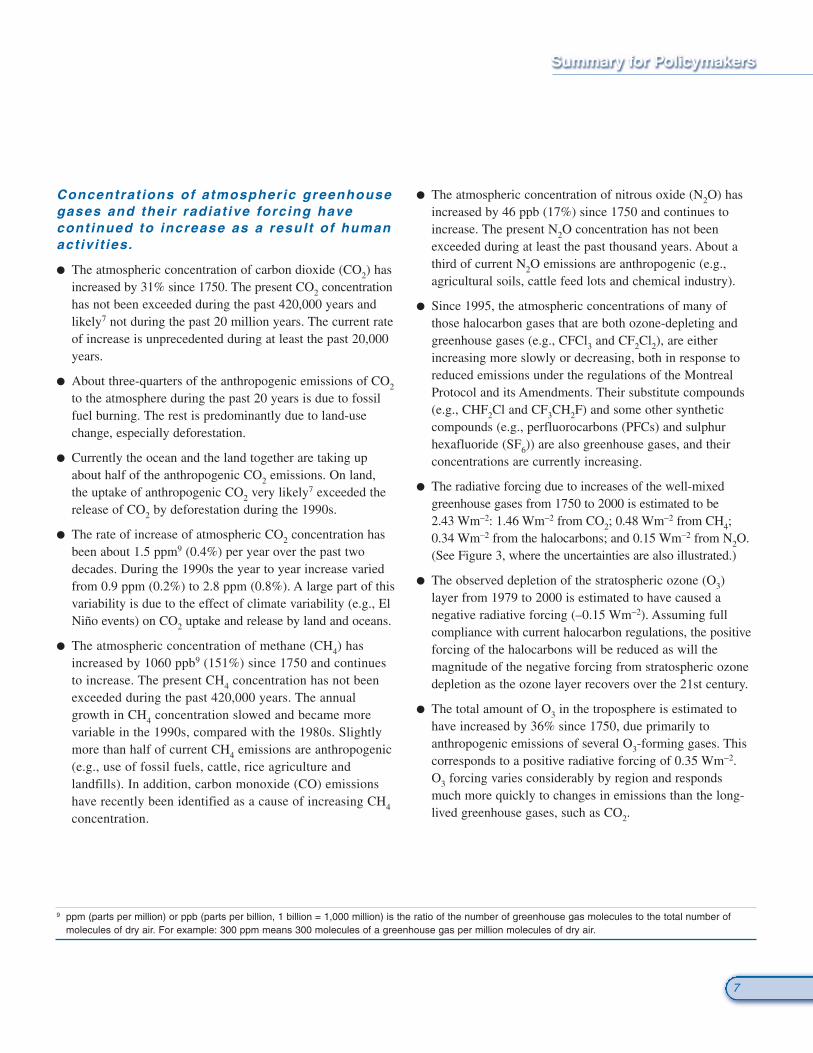
Concentrat ions of atmospheric greenhousegases and their radiat ive forcing havecontinued to increase as a result of humanact iv i t ies.

� The atmospheric concentration of carbon dioxide (CO2) hasincreased by 31% since 1750. The present CO2 concentrationhas not been exceeded during the past 420,000 years andlikely7 not during the past 20 million years. The current rateof increase is unprecedented during at least the past 20,000years.

� About three-quarters of the anthropogenic emissions of CO2

to the atmosphere during the past 20 years is due to fossilfuel burning. The rest is predominantly due to land-usechange, especially deforestation.

� Currently the ocean and the land together are taking upabout half of the anthropogenic CO2 emissions. On land,the uptake of anthropogenic CO2 very likely7 exceeded therelease of CO2 by deforestation during the 1990s.

� The rate of increase of atmospheric CO2 concentration hasbeen about 1.5 ppm9 (0.4%) per year over the past twodecades. During the 1990s the year to year increase variedfrom 0.9 ppm (0.2%) to 2.8 ppm (0.8%). A large part of thisvariability is due to the effect of climate variability (e.g., ElNiño events) on CO2 uptake and release by land and oceans.

� The atmospheric concentration of methane (CH4) hasincreased by 1060 ppb9 (151%) since 1750 and continuesto increase. The present CH4 concentration has not beenexceeded during the past 420,000 years. The annualgrowth in CH4 concentration slowed and became morevariable in the 1990s, compared with the 1980s. Slightlymore than half of current CH4 emissions are anthropogenic(e.g., use of fossil fuels, cattle, rice agriculture andlandfills). In addition, carbon monoxide (CO) emissionshave recently been identified as a cause of increasing CH4

concentration.

� The atmospheric concentration of nitrous oxide (N2O) hasincreased by 46 ppb (17%) since 1750 and continues toincrease. The present N2O concentration has not beenexceeded during at least the past thousand years. About athird of current N2O emissions are anthropogenic (e.g.,agricultural soils, cattle feed lots and chemical industry).

� Since 1995, the atmospheric concentrations of many ofthose halocarbon gases that are both ozone-depleting andgreenhouse gases (e.g., CFCl3 and CF2Cl2), are eitherincreasing more slowly or decreasing, both in response toreduced emissions under the regulations of the MontrealProtocol and its Amendments. Their substitute compounds(e.g., CHF2Cl and CF3CH2F) and some other syntheticcompounds (e.g., perfluorocarbons (PFCs) and sulphurhexafluoride (SF6)) are also greenhouse gases, and theirconcentrations are currently increasing.

� The radiative forcing due to increases of the well-mixedgreenhouse gases from 1750 to 2000 is estimated to be 2.43 Wm−2: 1.46 Wm−2 from CO2; 0.48 Wm−2 from CH4;0.34 Wm−2 from the halocarbons; and 0.15 Wm−2 from N2O.(See Figure 3, where the uncertainties are also illustrated.)

� The observed depletion of the stratospheric ozone (O3)layer from 1979 to 2000 is estimated to have caused anegative radiative forcing (–0.15 Wm−2). Assuming fullcompliance with current halocarbon regulations, the positiveforcing of the halocarbons will be reduced as will themagnitude of the negative forcing from stratospheric ozonedepletion as the ozone layer recovers over the 21st century.

� The total amount of O3 in the troposphere is estimated tohave increased by 36% since 1750, due primarily to anthropogenic emissions of several O3-forming gases. Thiscorresponds to a positive radiative forcing of 0.35 Wm−2. O3 forcing varies considerably by region and respondsmuch more quickly to changes in emissions than the long-lived greenhouse gases, such as CO2.

9 ppm (parts per million) or ppb (parts per billion, 1 billion = 1,000 million) is the ratio of the number of greenhouse gas molecules to the total number of molecules of dry air. For example: 300 ppm means 300 molecules of a greenhouse gas per million molecules of dry air.

7

Level of Scientific Understanding

−2

−1

0

1

2

3

Rad

iativ

e fo

rcin

g (

Wat

ts p

er s

quar

e m

etre

)

Coo

ling

War

min

g

The global mean radiative forcing of the climate system for the year 2000, relative to 1750

High Medium Medium Low VeryLow

VeryLow

VeryLow

VeryLow

VeryLow

VeryLow

CO2

VeryLow

CH4

N2OHalocarbons

Stratosphericozone

Troposphericozone

Sulphate

Blackcarbon from

fossilfuel

burning

Organic carbon

from fossilfuel

burning

Biomassburning

Contrails

SolarMineral

Dust

Aerosolindirect effect

Land-use

(albedo) only

Aviation-induced

Cirrus

VeryLow

Aerosols

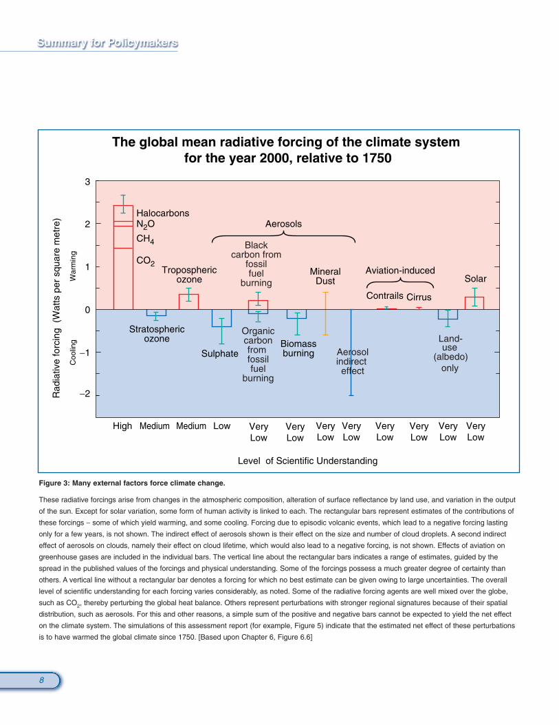
Figure 3: Many external factors force climate change.

These radiative forcings arise from changes in the atmospheric composition, alteration of surface reflectance by land use, and variation in the output

of the sun. Except for solar variation, some form of human activity is linked to each. The rectangular bars represent estimates of the contributions of

these forcings − some of which yield warming, and some cooling. Forcing due to episodic volcanic events, which lead to a negative forcing lasting

only for a few years, is not shown. The indirect effect of aerosols shown is their effect on the size and number of cloud droplets. A second indirect

effect of aerosols on clouds, namely their effect on cloud lifetime, which would also lead to a negative forcing, is not shown. Effects of aviation on

greenhouse gases are included in the individual bars. The vertical line about the rectangular bars indicates a range of estimates, guided by the

spread in the published values of the forcings and physical understanding. Some of the forcings possess a much greater degree of certainty than

others. A vertical line without a rectangular bar denotes a forcing for which no best estimate can be given owing to large uncertainties. The overall

level of scientific understanding for each forcing varies considerably, as noted. Some of the radiative forcing agents are well mixed over the globe,

such as CO2, thereby perturbing the global heat balance. Others represent perturbations with stronger regional signatures because of their spatial

distribution, such as aerosols. For this and other reasons, a simple sum of the positive and negative bars cannot be expected to yield the net effect

on the climate system. The simulations of this assessment report (for example, Figure 5) indicate that the estimated net effect of these perturbations

is to have warmed the global climate since 1750. [Based upon Chapter 6, Figure 6.6]

8

Anthropogenic aerosols are short- l ived andmostly produce negat ive radiat ive forcing.

� The major sources of anthropogenic aerosols are fossil fueland biomass burning. These sources are also linked todegradation of air quality and acid deposition.

� Since the SAR, significant progress has been achieved inbetter characterising the direct radiative roles of differenttypes of aerosols. Direct radiative forcing is estimated to be−0.4 Wm−2 for sulphate, −0.2 Wm−2 for biomass burningaerosols, −0.1 Wm−2 for fossil fuel organic carbon and +0.2 Wm−2 for fossil fuel black carbon aerosols. There ismuch less confidence in the ability to quantify the totalaerosol direct effect, and its evolution over time, than thatfor the gases listed above. Aerosols also vary considerablyby region and respond quickly to changes in emissions.

� In addition to their direct radiative forcing, aerosols have anindirect radiative forcing through their effects on clouds.There is now more evidence for this indirect effect, which isnegative, although of very uncertain magnitude.

Natural factors have made smal l contr ibut ions to radiat ive forcing over thepast century.

� The radiative forcing due to changes in solar irradiance forthe period since 1750 is estimated to be about +0.3 Wm−2,most of which occurred during the first half of the 20thcentury. Since the late 1970s, satellite instruments haveobserved small oscillations due to the 11-year solar cycle.Mechanisms for the amplification of solar effects onclimate have been proposed, but currently lack a rigoroustheoretical or observational basis.

� Stratospheric aerosols from explosive volcanic eruptionslead to negative forcing, which lasts a few years. Severalmajor eruptions occurred in the periods 1880 to 1920 and1960 to 1991.

� The combined change in radiative forcing of the two majornatural factors (solar variation and volcanic aerosols) isestimated to be negative for the past two, and possibly thepast four, decades.

Confidence in the abi l i ty of modelsto project future cl imate hasincreased.

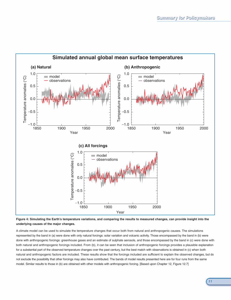
Complex physically-based climate models are required toprovide detailed estimates of feedbacks and of regionalfeatures. Such models cannot yet simulate all aspects ofclimate (e.g., they still cannot account fully for the observedtrend in the surface-troposphere temperature difference since1979) and there are particular uncertainties associated withclouds and their interaction with radiation and aerosols.Nevertheless, confidence in the ability of these models toprovide useful projections of future climate has improved dueto their demonstrated performance on a range of space andtime-scales.

� Understanding of climate processes and their incorporationin climate models have improved, including water vapour,sea-ice dynamics, and ocean heat transport.

� Some recent models produce satisfactory simulations ofcurrent climate without the need for non-physical adjustmentsof heat and water fluxes at the ocean-atmosphere interfaceused in earlier models.

� Simulations that include estimates of natural and anthropogenic forcing reproduce the observed large-scalechanges in surface temperature over the 20th century(Figure 4). However, contributions from some additionalprocesses and forcings may not have been included in themodels. Nevertheless, the large-scale consistency betweenmodels and observations can be used to provide anindependent check on projected warming rates over the nextfew decades under a given emissions scenario.

� Some aspects of model simulations of ENSO, monsoonsand the North Atlantic Oscillation, as well as selectedperiods of past climate, have improved.

9

There is new and stronger evidencethat most of the warming observedover the last 50 years is at tr ib-utable to human act iv i t ies.

The SAR concluded: “The balance of evidence suggests adiscernible human influence on global climate”. That reportalso noted that the anthropogenic signal was still emerging fromthe background of natural climate variability. Since the SAR,progress has been made in reducing uncertainty, particularlywith respect to distinguishing and quantifying the magnitudeof responses to different external influences. Although manyof the sources of uncertainty identified in the SAR still remainto some degree, new evidence and improved understandingsupport an updated conclusion.

� There is a longer and more closely scrutinised temperaturerecord and new model estimates of variability. The warmingover the past 100 years is very unlikely7 to be due tointernal variability alone, as estimated by current models.Reconstructions of climate data for the past 1,000 years(Figure 1b) also indicate that this warming was unusual andis unlikely7 to be entirely natural in origin.

� There are new estimates of the climate response to naturaland anthropogenic forcing, and new detection techniqueshave been applied. Detection and attribution studies consis-tently find evidence for an anthropogenic signal in theclimate record of the last 35 to 50 years.

� Simulations of the response to natural forcings alone (i.e.,the response to variability in solar irradiance and volcaniceruptions) do not explain the warming in the second half ofthe 20th century (see for example Figure 4a). However, theyindicate that natural forcings may have contributed to theobserved warming in the first half of the 20th century.

� The warming over the last 50 years due to anthropogenicgreenhouse gases can be identified despite uncertainties inforcing due to anthropogenic sulphate aerosol and naturalfactors (volcanoes and solar irradiance). The anthropogenicsulphate aerosol forcing, while uncertain, is negative overthis period and therefore cannot explain the warming.Changes in natural forcing during most of this period arealso estimated to be negative and are unlikely7 to explainthe warming.

� Detection and attribution studies comparing modelsimulated changes with the observed record can now takeinto account uncertainty in the magnitude of modelledresponse to external forcing, in particular that due touncertainty in climate sensitivity.

� Most of these studies find that, over the last 50 years, theestimated rate and magnitude of warming due to increasingconcentrations of greenhouse gases alone are comparablewith, or larger than, the observed warming. Furthermore,most model estimates that take into account bothgreenhouse gases and sulphate aerosols are consistent withobservations over this period.

� The best agreement between model simulations andobservations over the last 140 years has been found whenall the above anthropogenic and natural forcing factors arecombined, as shown in Figure 4c. These results show thatthe forcings included are sufficient to explain the observedchanges, but do not exclude the possibility that otherforcings may also have contributed.

In the light of new evidence and taking into account theremaining uncertainties, most of the observed warming overthe last 50 years is likely7 to have been due to the increase ingreenhouse gas concentrations.

Furthermore, it is very likely7 that the 20th century warminghas contributed significantly to the observed sea level rise,through thermal expansion of sea water and widespread loss ofland ice. Within present uncertainties, observations and modelsare both consistent with a lack of significant acceleration ofsea level rise during the 20th century.

10

Tem

pera

ture

ano

mal

ies

(°C

)

Tem

pera

ture

ano

mal

ies

(°C

)

(a) Natural (b) Anthropogenic

(c) All forcings

1850 1900 1950 2000Year

−1.0

−0.5

0.0

0.5

1.0

Tem

pera

ture

ano

mal

ies

(°C

)

Simulated annual global mean surface temperatures

1850 1900 1950 2000Year

−1.0

−0.5

0.0

0.5

1.0

−1.0

−0.5

0.0

0.5

1.0

1850 1900 1950 2000Year

modelobservations

modelobservations

modelobservations

Figure 4: Simulating the Earth’s temperature variations, and comparing the results to measured changes, can provide insight into the

underlying causes of the major changes.

A climate model can be used to simulate the temperature changes that occur both from natural and anthropogenic causes. The simulations

represented by the band in (a) were done with only natural forcings: solar variation and volcanic activity. Those encompassed by the band in (b) were

done with anthropogenic forcings: greenhouse gases and an estimate of sulphate aerosols, and those encompassed by the band in (c) were done with

both natural and anthropogenic forcings included. From (b), it can be seen that inclusion of anthropogenic forcings provides a plausible explanation

for a substantial part of the observed temperature changes over the past century, but the best match with observations is obtained in (c) when both

natural and anthropogenic factors are included. These results show that the forcings included are sufficient to explain the observed changes, but do

not exclude the possibility that other forcings may also have contributed. The bands of model results presented here are for four runs from the same

model. Similar results to those in (b) are obtained with other models with anthropogenic forcing. [Based upon Chapter 12, Figure 12.7]

11

Human inf luences wi l l cont inue tochange atmospheric composit ionthroughout the 21st century.

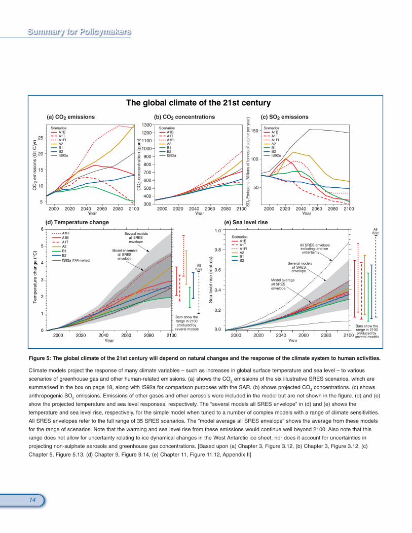
Models have been used to make projections of atmosphericconcentrations of greenhouse gases and aerosols, and hence offuture climate, based upon emissions scenarios from the IPCCSpecial Report on Emission Scenarios (SRES) (Figure 5).These scenarios were developed to update the IS92 series,which were used in the SAR and are shown for comparisonhere in some cases.

Greenhouse gases

� Emissions of CO2 due to fossil fuel burning are virtuallycertain7 to be the dominant influence on the trends inatmospheric CO2 concentration during the 21st century.

� As the CO2 concentration of the atmosphere increases, oceanand land will take up a decreasing fraction of anthropogenicCO2 emissions. The net effect of land and ocean climatefeedbacks as indicated by models is to further increaseprojected atmospheric CO2 concentrations, by reducingboth the ocean and land uptake of CO2.

� By 2100, carbon cycle models project atmospheric CO2

concentrations of 540 to 970 ppm for the illustrative SRESscenarios (90 to 250% above the concentration of 280 ppmin the year 1750), Figure 5b. These projections include theland and ocean climate feedbacks. Uncertainties, especiallyabout the magnitude of the climate feedback from theterrestrial biosphere, cause a variation of about −10 to+30% around each scenario. The total range is 490 to 1260ppm (75 to 350% above the 1750 concentration).

� Changing land use could influence atmospheric CO2

concentration. Hypothetically, if all of the carbon releasedby historical land-use changes could be restored to theterrestrial biosphere over the course of the century (e.g., byreforestation), CO2 concentration would be reduced by 40to 70 ppm.

� Model calculations of the concentrations of the non-CO2

greenhouse gases by 2100 vary considerably across theSRES illustrative scenarios, with CH4 changing by –190 to+1,970 ppb (present concentration 1,760 ppb), N2O changing

by +38 to +144 ppb (present concentration 316 ppb), totaltropospheric O3 changing by −12 to +62%, and a widerange of changes in concentrations of HFCs, PFCs and SF6,all relative to the year 2000. In some scenarios, total tropos-pheric O3 would become as important a radiative forcingagent as CH4 and, over much of the Northern Hemisphere,would threaten the attainment of current air quality targets.

� Reductions in greenhouse gas emissions and the gases thatcontrol their concentration would be necessary to stabiliseradiative forcing. For example, for the most importantanthropogenic greenhouse gas, carbon cycle models indicatethat stabilisation of atmospheric CO2 concentrations at 450,650 or 1,000 ppm would require global anthropogenic CO2

emissions to drop below 1990 levels, within a few decades,about a century, or about two centuries, respectively, andcontinue to decrease steadily thereafter. Eventually CO2

emissions would need to decline to a very small fraction ofcurrent emissions.

Aerosols

� The SRES scenarios include the possibility of either increasesor decreases in anthropogenic aerosols (e.g., sulphateaerosols (Figure 5c), biomass aerosols, black and organiccarbon aerosols) depending on the extent of fossil fuel useand policies to abate polluting emissions. In addition,natural aerosols (e.g., sea salt, dust and emissions leading tothe production of sulphate and carbon aerosols) areprojected to increase as a result of changes in climate.

Radiat ive forcing over the 21st century

� For the SRES illustrative scenarios, relative to the year2000, the global mean radiative forcing due to greenhousegases continues to increase through the 21st century, withthe fraction due to CO2 projected to increase from slightlymore than half to about three quarters. The change in thedirect plus indirect aerosol radiative forcing is projected tobe smaller in magnitude than that of CO2.

12

Global average temperature and sealevel are projected to r ise under al lIPCC SRES scenarios.

In order to make projections of future climate, modelsincorporate past, as well as future emissions of greenhousegases and aerosols. Hence, they include estimates of warmingto date and the commitment to future warming from pastemissions.

Temperature

� The globally averaged surface temperature is projected toincrease by 1.4 to 5.8°C (Figure 5d) over the period 1990 to2100. These results are for the full range of 35 SRESscenarios, based on a number of climate models10,11.

� Temperature increases are projected to be greater than thosein the SAR, which were about 1.0 to 3.5°C based on the sixIS92 scenarios. The higher projected temperatures and thewider range are due primarily to the lower projectedsulphur dioxide emissions in the SRES scenarios relative tothe IS92 scenarios.

� The projected rate of warming is much larger than theobserved changes during the 20th century and is very likely7

to be without precedent during at least the last 10,000 years,based on palaeoclimate data.

� By 2100, the range in the surface temperature responseacross the group of climate models run with a givenscenario is comparable to the range obtained from a singlemodel run with the different SRES scenarios.

� On timescales of a few decades, the current observed rate ofwarming can be used to constrain the projected response toa given emissions scenario despite uncertainty in climatesensitivity. This approach suggests that anthropogenic

warming is likely7 to lie in the range of 0.1 to 0.2°C perdecade over the next few decades under the IS92a scenario,similar to the corresponding range of projections of thesimple model used in Figure 5d.

� Based on recent global model simulations, it is very likely7

that nearly all land areas will warm more rapidly than theglobal average, particularly those at northern high latitudesin the cold season. Most notable of these is the warming inthe northern regions of North America, and northern andcentral Asia, which exceeds global mean warming in eachmodel by more than 40%. In contrast, the warming is lessthan the global mean change in south and southeast Asia insummer and in southern South America in winter.

� Recent trends for surface temperature to become more El Niño-like in the tropical Pacific, with the eastern tropicalPacific warming more than the western tropical Pacific,with a corresponding eastward shift of precipitation, areprojected to continue in many models.

Precipi tat ion

� Based on global model simulations and for a wide range ofscenarios, global average water vapour concentration andprecipitation are projected to increase during the 21stcentury. By the second half of the 21st century, it is likely7

that precipitation will have increased over northern mid- tohigh latitudes and Antarctica in winter. At low latitudesthere are both regional increases and decreases over landareas. Larger year to year variations in precipitation arevery likely7 over most areas where an increase in meanprecipitation is projected.

10 Complex physically based climate models are the main tool for projecting future climate change. In order to explore the full range of scenarios, these are complemented by simple climate models calibrated to yield an equivalent response in temperature and sea level to complex climate models. These projections are obtained using a simple climate model whose climate sensitivity and ocean heat uptake are calibrated to each of seven complex climate models. The climate sensitivity used in the simple model ranges from 1.7 to 4.2°C, which is comparable to the commonly accepted range of 1.5 to 4.5°C.

11 This range does not include uncertainties in the modelling of radiative forcing, e.g. aerosol forcing uncertainties. A small carbon-cycle climate feedback is included.

13

2000 2020 2040 2060 2080 2100

5

10

15

20

25

CO

2 em

issi

ons

(Gt C

/yr)

Several modelsall SRESenvelope

All SRES envelopeincluding land-iceuncertainty

Model averageall SRESenvelope

AllIS92

Bars show therange in 2100produced by

several models

(a) CO2 emissions (b) CO2 concentrations (c) SO2 emissions

(e) Sea level rise

2000 2020 2040 2060 2080 2100YearYearYear

50

100

150

SO2

Emis

sion

s (M

illion

s of

tonn

es o

f sul

phur

per

yea

r)

A1BA1TA1FIA2B1B2IS92a

ScenariosA1BA1TA1FIA2B1B2IS92a

ScenariosA1BA1TA1FIA2B1B2IS92a

Scenarios

A1BA1TA1FIA2B1B2

Scenarios

CO

2 co

ncen

trat

ion

(ppm

)

300

400

500

600

700

800

900

1000

1100

1200

1300

2000 2020 2040 2060 2080 2100

2000 2020 2040 2060 2080 2100Year

0.0

0.2

0.4

0.6

0.8

1.0

Sea

leve

l ris

e (m

etre

s)

The global climate of the 21st century

(d) Temperature change

AllIS92

2000 2020 2040 2060 2080 2100Year

0

1

2

3

4

5

6

Tem

pera

ture

cha

nge

(°C

)

A1FIA1BA1TA2B1B2IS92a (TAR method)


Model ensembleall SRESenvelope


several models

Figure 5: The global climate of the 21st century will depend on natural changes and the response of the climate system to human activities.

Climate models project the response of many climate variables – such as increases in global surface temperature and sea level – to various

scenarios of greenhouse gas and other human-related emissions. (a) shows the CO2 emissions of the six illustrative SRES scenarios, which are

summarised in the box on page 18, along with IS92a for comparison purposes with the SAR. (b) shows projected CO2 concentrations. (c) shows

anthropogenic SO2 emissions. Emissions of other gases and other aerosols were included in the model but are not shown in the figure. (d) and (e)

show the projected temperature and sea level responses, respectively. The “several models all SRES envelope” in (d) and (e) shows the

temperature and sea level rise, respectively, for the simple model when tuned to a number of complex models with a range of climate sensitivities.

All SRES envelopes refer to the full range of 35 SRES scenarios. The “model average all SRES envelope” shows the average from these models

for the range of scenarios. Note that the warming and sea level rise from these emissions would continue well beyond 2100. Also note that this

range does not allow for uncertainty relating to ice dynamical changes in the West Antarctic ice sheet, nor does it account for uncertainties in

projecting non-sulphate aerosols and greenhouse gas concentrations. [Based upon (a) Chapter 3, Figure 3.12, (b) Chapter 3, Figure 3.12, (c)

Chapter 5, Figure 5.13, (d) Chapter 9, Figure 9.14, (e) Chapter 11, Figure 11.12, Appendix II]

14

Extreme Events

Table 1 depicts an assessment of confidence in observedchanges in extremes of weather and climate during the latterhalf of the 20th century (left column) and in projected changesduring the 21st century (right column)a. This assessment relieson observational and modelling studies, as well as the physicalplausibility of future projections across all commonly-usedscenarios and is based on expert judgement7.

� For some other extreme phenomena, many of which mayhave important impacts on the environment and society,there is currently insufficient information to assess recenttrends, and climate models currently lack the spatial detailrequired to make confident projections. For example, verysmall-scale phenomena, such as thunderstorms, tornadoes,hail and lightning, are not simulated in climate models.

a For more details see Chapter 2 (observations) and Chapter 9, 10 (projections).

b For other areas, there are either insufficient data or conflicting analyses.

c Past and future changes in tropical cyclone location and frequency are uncertain.

12 Heat index: A combination of temperature and humidity that measures effects on human comfort.

Confidence in observed changes Changes in Phenomenon Confidence in projected changes(latter half of the 20th century) (during the 21st century)

Likely7 Higher maximum temperatures and more Very likely7

hot days over nearly all land areas

Very likely7 Higher minimum temperatures, fewer Very likely7

cold days and frost days over nearly all land areas

Very likely7 Reduced diurnal temperature range over Very likely7

most land areas

Likely7, over many areas Increase of heat index12 over land areas Very likely7, over most areas

Likely7, over many Northern Hemisphere More intense precipitation eventsb Very likely7, over many areasmid- to high latitude land areas

Likely7, in a few areas Increased summer continental drying Likely7, over most mid-latitude continentaland associated risk of drought interiors. (Lack of consistent projections

in other areas)

Not observed in the few analyses Increase in tropical cyclone peak wind Likely7, over some areasavailable intensitiesc

Insufficient data for assessment Increase in tropical cyclone mean and Likely7, over some areaspeak precipitation intensitiesc

15

Table 1: Estimates of confidence in observed and projected changes in extreme weather and climate events.

El Niño

� Confidence in projections of changes in future frequency,amplitude, and spatial pattern of El Niño events in thetropical Pacific is tempered by some shortcomings in howwell El Niño is simulated in complex models. Currentprojections show little change or a small increase inamplitude for El Niño events over the next 100 years.

� Even with little or no change in El Niño amplitude,global warming is likely7 to lead to greater extremes ofdrying and heavy rainfall and increase the risk ofdroughts and floods that occur with El Niño events inmany different regions.

Monsoons

� It is likely7 that warming associated with increasinggreenhouse gas concentrations will cause an increase ofAsian summer monsoon precipitation variability. Changesin monsoon mean duration and strength depend on thedetails of the emission scenario. The confidence in suchprojections is also limited by how well the climatemodels simulate the detailed seasonal evolution of themonsoons.

Thermohal ine circulat ion

� Most models show weakening of the ocean thermohalinecirculation which leads to a reduction of the heattransport into high latitudes of the Northern Hemisphere.However, even in models where the thermohalinecirculation weakens, there is still a warming over Europedue to increased greenhouse gases. The currentprojections using climate models do not exhibit acomplete shut-down of the thermohaline circulation by2100. Beyond 2100, the thermohaline circulation couldcompletely, and possibly irreversibly, shut-down in eitherhemisphere if the change in radiative forcing is largeenough and applied long enough.

Snow and ice

� Northern Hemisphere snow cover and sea-ice extent areprojected to decrease further.

� Glaciers and ice caps are projected to continue theirwidespread retreat during the 21st century.

� The Antarctic ice sheet is likely7 to gain mass because ofgreater precipitation, while the Greenland ice sheet islikely7 to lose mass because the increase in runoff willexceed the precipitation increase.

� Concerns have been expressed about the stability of theWest Antarctic ice sheet because it is grounded below sealevel. However, loss of grounded ice leading to substantialsea level rise from this source is now widely agreed to bevery unlikely7 during the 21st century, although itsdynamics are still inadequately understood, especially forprojections on longer time-scales.

Sea level

� Global mean sea level is projected to rise by 0.09 to 0.88metres between 1990 and 2100, for the full range ofSRES scenarios. This is due primarily to thermalexpansion and loss of mass from glaciers and ice caps(Figure 5e). The range of sea level rise presented in theSAR was 0.13 to 0.94 metres based on the IS92scenarios. Despite the higher temperature changeprojections in this assessment, the sea level projectionsare slightly lower, primarily due to the use of improvedmodels, which give a smaller contribution from glaciersand ice sheets.

16

Anthropogenic cl imate change wi l lpersist for many centur ies.

� Emissions of long-lived greenhouse gases (i.e., CO2, N2O,PFCs, SF6) have a lasting effect on atmosphericcomposition, radiative forcing and climate. For example,several centuries after CO2 emissions occur, about a quarterof the increase in CO2 concentration caused by theseemissions is still present in the atmosphere.

� After greenhouse gas concentrations have stabilised, globalaverage surface temperatures would rise at a rate of only afew tenths of a degree per century rather than severaldegrees per century as projected for the 21st centurywithout stabilisation. The lower the level at which concentrations are stabilised, the smaller the totaltemperature change.

� Global mean surface temperature increases and rising sealevel from thermal expansion of the ocean are projected tocontinue for hundreds of years after stabilisation ofgreenhouse gas concentrations (even at present levels),owing to the long timescales on which the deep oceanadjusts to climate change.

� Ice sheets will continue to react to climate warming andcontribute to sea level rise for thousands of years afterclimate has been stabilised. Climate models indicate thatthe local warming over Greenland is likely7 to be one tothree times the global average. Ice sheet models project thata local warming of larger than 3°C, if sustained formillennia, would lead to virtually a complete melting of theGreenland ice sheet with a resulting sea level rise of about7 metres. A local warming of 5.5°C, if sustained for 1,000years, would be likely7 to result in a contribution fromGreenland of about 3 metres to sea level rise.

� Current ice dynamic models suggest that the West Antarcticice sheet could contribute up to 3 metres to sea level riseover the next 1,000 years, but such results are stronglydependent on model assumptions regarding climate changescenarios, ice dynamics and other factors.

Further act ion is required toaddress remaining gaps ininformation and understanding.

Further research is required to improve the ability to detect,attribute and understand climate change, to reduce uncertaintiesand to project future climate changes. In particular, there is aneed for additional systematic and sustained observations,modelling and process studies. A serious concern is the declineof observational networks. The following are high priorityareas for action.

� Systematic observations and reconstructions:

– Reverse the decline of observational networks in many parts of the world.

– Sustain and expand the observational foundation for climate studies by providing accurate, long-term,consistent data including implementation of a strategy for integrated global observations.

– Enhance the development of reconstructions of past climate periods.

– Improve the observations of the spatial distribution of greenhouse gases and aerosols.

� Modelling and process studies:

– Improve understanding of the mechanisms and factors leading to changes in radiative forcing.

– Understand and characterise the important unresolved processes and feedbacks, both physical and biogeo-chemical, in the climate system.

– Improve methods to quantify uncertainties of climate projections and scenarios, including long-term ensemble simulations using complex models.

– Improve the integrated hierarchy of global and regional climate models with a focus on the simulation of climate variability, regional climate changes and extreme events.

– Link more effectively models of the physical climate and the biogeochemical system, and in turn improve coupling with descriptions of human activities.

17

Cutting across these foci are crucial needs associated withstrengthening international co-operation and co-ordination inorder to better utilise scientific, computational and observationalresources. This should also promote the free exchange of dataamong scientists. A special need is to increase the observationaland research capacities in many regions, particularly indeveloping countries. Finally, as is the goal of this assessment,there is a continuing imperative to communicate researchadvances in terms that are relevant to decision making.

The Emissions Scenarios of the Special Report on Emissions Scenarios(SRES)

A1. The A1 storyline and scenario family describes a future world of very rapid economic growth, global population thatpeaks in mid-century and declines thereafter, and the rapid introduction of new and more efficient technologies. Majorunderlying themes are convergence among regions, capacity building and increased cultural and social interactions, with asubstantial reduction in regional differences in per capita income. The A1 scenario family develops into three groups thatdescribe alternative directions of technological change in the energy system. The three A1 groups are distinguished by theirtechnological emphasis: fossil intensive (A1FI), non-fossil energy sources (A1T), or a balance across all sources (A1B) (wherebalanced is defined as not relying too heavily on one particular energy source, on the assumption that similar improvementrates apply to all energy supply and end use technologies).

A2. The A2 storyline and scenario family describes a very heterogeneous world. The underlying theme is self-reliance andpreservation of local identities. Fertility patterns across regions converge very slowly, which results in continuously increasingpopulation. Economic development is primarily regionally oriented and per capita economic growth and technological changemore fragmented and slower than other storylines.

B1. The B1 storyline and scenario family describes a convergent world with the same global population, that peaks in mid-century and declines thereafter, as in the A1 storyline, but with rapid change in economic structures toward a service andinformation economy, with reductions in material intensity and the introduction of clean and resource-efficient technologies.The emphasis is on global solutions to economic, social and environmental sustainability, including improved equity, butwithout additional climate initiatives.

B2. The B2 storyline and scenario family describes a world in which the emphasis is on local solutions to economic, socialand environmental sustainability. It is a world with continuously increasing global population, at a rate lower than A2,intermediate levels of economic development, and less rapid and more diverse technological change than in the B1 and A1storylines. While the scenario is also oriented towards environmental protection and social equity, it focuses on local andregional levels.

An illustrative scenario was chosen for each of the six scenario groups A1B, A1FI, A1T, A2, B1 and B2. All should beconsidered equally sound.

The SRES scenarios do not include additional climate initiatives, which means that no scenarios are included that explicitlyassume implementation of the United Nations Framework Convention on Climate Change or the emissions targets of theKyoto Protocol.

18

Source Information: Summary forPol icymakers

This appendix provides the cross-reference of the topics in theSummary for Policymakers (page and bullet point topic) to thesections of the chapters of the full report that containexpanded information about the topic.

An increasing body of observat ions gives acol lect ive picture of a warming world andother changes in the cl imate system.

SPM Page Cross-Reference: SPM Topic – Chapter Section

2 The global average surface temperature has increased over the 20th century by about 0.6°C.� Chapter 2.2.2 � Chapter 2.2.2 � Chapter 2.3� Chapter 2.2.2

4 Temperatures have risen during the past four decades in the lowest 8 kilometres of the atmosphere. � Chapter 2.2.3 and 2.2.4� Chapter 2.2.3 and 2.2.4 � Chapter 2.2.3, 2.2.4 and Chapter 12.3.2

4 Snow cover and ice extent have decreased. All three bullet points: Chapter 2.2.5 and 2.2.6

4 Global average sea level has risen and ocean heat content has increased. � Chapter 11.3.2 � Chapter 2.2.2 and Chapter 11.2.1

4 − 5 Changes have also occurred in other important aspects of climate. � Chapter 2.5.2� Chapter 2.7.2 � Chapter 2.2.2 and 2.5.5� Chapter 2.7.2 � Chapter 2.6.2 and 2.6.3� Chapter 2.7.3 � Chapter 2.7.3

5 Some important aspects of climate appear not to have changed. � Chapter 2.2.2 � Chapter 2.2.5 � Chapter 2.7.3 � Chapter 2.7.3

Emissions of greenhouse gases andaerosols due to human act iv i t ies cont inueto al ter the atmosphere in ways that areexpected to affect the cl imate system.


5 Chapeau: “Changes in climate occur …”Chapter 1, Chapter 3.1, Chapter 4.1, Chapter 5.1,Chapter 6.1, 6.2, 6.9, 6.11 and 6.13

7 Concentrations of atmospheric greenhouse gases and their radiative forcing have continued to increase as a result of human activities.

Carbon dioxide: � Chapter 3.3.1, 3.3.2, 3.3.3 and 3.5.1 � Chapter 3.5.1 � Chapter 3.2.2, 3.2.3, 3.5.1 and Table 3.1� Chapter 3.5.1 and 3.5.2

Methane: � Chapter 4.2.1

Nitrous oxide: � Chapter 4.2.1

Halocarbons: � Chapter 4.2.2

Radiative forcing of well-mixed gases:� Chapter 4.2.1 and Chapter 6.3

Stratospheric ozone: � Chapter 4.2.2 and Chapter 6.4

Tropospheric ozone: � Chapter 4.2.4 and Chapter 6.5

9 Anthropogenic aerosols are short-lived and mostly produce negative radiative forcing. � Chapter 5.2 and 5.5.4 � Chapter 5.1, 5.2 and Chapter 6.7 � Chapter 5.3.2, 5.4.3 and Chapter 6.8

9 Natural factors have made small contributions to radiative forcing over the past century.� Chapter 6.11 and 6.15.1 � Chapter 6.9 and 6.15.1� Chapter 6.15.1

19

Confidence in the abi l i ty of models toproject future cl imate has increased.


9 Chapeau: “Complex physically-based …”Chapter 8.3.2, 8.5.1, 8.6.1, 8.10.3 and Chapter 12.3.2

9 � Chapter 7.2.1, 7.5.2 and 7.6.1 � Chapter 8.4.2 � Chapter 8.6.3 and Chapter 12.3.2� Chapter 8.5.5, 8.7.1 and 8.7.5

There is new and stronger evidence thatmost of the warming observed over the last50 years is attr ibutable to human activi t ies.


10 Chapeau: “The SAR concluded: The balance of evidence suggests …” Chapter 12.1.2 and 12.6

10 � Chapter 12.2.2, 12.4.3 and 12.6� Chapter 12.4.1, 12.4.2, 12.4.3 and 12.6� Chapter 12.2.3, 12.4.1, 12.4.2, 12.4.3 and 12.6 � Chapter 12.4.3 and 12.6. � Chapter 12.6� Chapter 12.4.3 � Chapter 12.4.3 and 12.6

10 “In the light of new evidence and taking into account the …” Chapter 12.4 and 12.6

10 “Furthermore, it is very likely that the 20th century warming has …” Chapter 11.4

Human inf luences wi l l cont inue to changeatmospheric composit ion throughout the21st century.


12 Chapeau: “Models have been used to make projections …” Chapter 4.4.5 and Appendix II

12 Greenhouse gases � Chapter 3.7.3 and Appendix II� Chapter 3.7.1, 3.7.2, 3.7.3 and Appendix II� Chapter 3.7.3 and Appendix II� Chapter 3.2.2 and Appendix II� Chapter 4.4.5, 4.5, 4.6 and Appendix II� Chapter 3.7.3

12 Aerosols � Chapter 5.5.2, 5.5.3 and Appendix II

12 Radiative forcing over the 21st century� Chapter 6.15.2 and Appendix II

Global average temperature and sea levelare projected to r ise under al l IPCC SRESscenarios.


13 Temperature � Chapter 9.3.3 � Chapter 9.3.3 � Chapter 2.2.2, 2.3.2 and 2.4 � Chapter 9.3.3 and Chapter 10.3.2 � Chapter 8.6.1, Chapter 12.4.3, Chapter 13.5.1 and 13.5.2� Chapter 10.3.2 and Box 10.1 � Chapter 9.3.2

13 Precipitation � Chapter 9.3.1, 9.3.6, Chapter 10.3.2 and Box 10.1

15 Extreme events Table 1: Chapter 2.1, 2.2, 2.5,2.7.2, 2.7.3, Chapter 9.3.6 and Chapter 10.3.2 � Chapter 2.7.3 and Chapter 9.3.6

16 El Niño � Chapter 9.3.5 � Chapter 9.3.5

16 Monsoons � Chapter 9.3.5

16 Thermohaline circulation � Chapter 9.3.4

16 Snow and ice � Chapter 9.3.2 � Chapter 11.5.1 � Chapter 11.5.1 � Chapter 11.5.4

16 Sea level � Chapter 11.5.1

Anthropogenic cl imate change wi l l persistfor many centur ies.


17 � Chapter 3.2.3, Chapter 4.4 and Chapter 6.15 � Chapter 9.3.3 and 9.3.4 � Chapter 11.5.4 � Chapter 11.5.4 � Chapter 11.5.4

Further work is required to addressremaining gaps in information andunderstanding.


17 – 18 All bullet points: Chapter 14, Executive Summary

20

A repor t accepted by Working Group I of the IPCC but not approved in detai l

“Acceptance” of IPCC Reports at a Session of the Working Group or Panel signifies that thematerial has not been subject to line by line discussion and agreement, but nevertheless

presents a comprehensive, objective and balanced view of the subject matter.

21

Technical Summary

Co-ordinat ing Lead AuthorsD.L. Albritton (USA), L.G. Meira Filho (Brazil)

Lead AuthorsU. Cubasch (Germany), X. Dai (China), Y. Ding (China), D.J. Griggs (UK), B. Hewitson (South Africa), J.T. Houghton (UK),I. Isaksen (Norway), T. Karl (USA), M. McFarland (USA), V.P. Meleshko (Russia), J.F.B. Mitchell (UK), M. Noguer (UK),B.S. Nyenzi (Tanzania), M. Oppenheimer (USA), J.E. Penner (USA), S. Pollonais (Trinidad and Tobago),T. Stocker (Switzerland), K.E. Trenberth (USA)

Contr ibut ing AuthorsM.R. Allen, (UK), A.P.M. Baede (Netherlands), J.A. Church (Australia), D.H. Ehhalt (Germany), C.K. Folland (UK),F. Giorgi (Italy), J.M. Gregory (UK), J.M. Haywood (UK), J.I. House (Germany), M. Hulme (UK), V.J. Jaramillo (Mexico),A. Jayaraman (India), C.A. Johnson (UK), S. Joussaume (France), D.J. Karoly (Australia), H. Kheshgi (USA),C. Le Quéré (France), L.J. Mata (Germany), B.J. McAvaney (Australia), L.O. Mearns (USA), G.A. Meehl (USA),B. Moore III (USA), R.K. Mugara (Zambia), M. Prather (USA), C. Prentice (Germany), V. Ramaswamy (USA),S.C.B. Raper (UK), M.J. Salinger (New Zealand), R. Scholes (S. Africa), S. Solomon (USA), R. Stouffer (USA),M-X. Wang (China), R.T. Watson (USA), K-S. Yap (Malaysia)

Review EditorsF. Joos (Switzerland), A. Ramirez-Rojas (Venzuela), J.M.R. Stone (Canada), J. Zillman (Australia)

A. Introduct ion

A.1 The IPCC and i ts Working Groups

The Intergovernmental Panel on Climate Change (IPCC) wasestablished by the World Meteorological Organisation (WMO)and the United Nations Environment Programme (UNEP) in1988. The aim was, and remains, to provide an assessment ofthe understanding of all aspects of climate change1, includinghow human activities can cause such changes and can beimpacted by them. It had become widely recognised thathuman-influenced emissions of greenhouse gases have thepotential to alter the climate system (see Box 1), with possibledeleterious or beneficial effects. It was also recognised thataddressing such global issues required organisation on a globalscale, including assessment of the understanding of the issueby the worldwide expert communities.

At its first session, the IPCC was organised into three WorkingGroups. The current remits of the Working Groups are forWorking Group I to address the scientific aspects of theclimate system and climate change, Working Group II toaddress the impacts of and adaptations to climate change, andWorking Group III to address the options for the mitigation ofclimate change. The IPCC provided its first major assessmentreport in 1990 and its second major assessment report in 1996.

The IPCC reports are (i) up-to-date descriptions of the knownsand unknowns of the climate system and related factors, (ii)based on the knowledge of the international expertcommunities, (iii) produced by an open and peer-reviewedprofessional process, and (iv) based upon scientific publicationswhose findings are summarised in terms useful to decisionmakers. While the assessed information is policy relevant, theIPCC does not establish or advocate public policy.

The scope of the assessments of Working Group I includesobservations of the current changes and trends in the climate

system, a reconstruction of past changes and trends, anunderstanding of the processes involved in those changes, andthe incorporation of this knowledge into models that can attributethe causes of changes and that can provide simulation of naturaland human-induced future changes in the climate system.

A.2 The First and Second AssessmentRepor ts of Working Group I

In the First Assessment Report in 1990, Working Group I broadlydescribed the status of the understanding of the climate systemand climate change that had been gained over the precedingdecades of research. Several major points were emphasised. Thegreenhouse effect is a natural feature of the planet, and itsfundamental physics is well understood. The atmosphericabundances of greenhouse gases were increasing, due largely tohuman activities. Continued future growth in greenhouse gasemissions was predicted to lead to significant increases in theaverage surface temperature of the planet, increases that wouldexceed the natural variation of the past several millennia and thatcould be reversed only slowly. The past century had, at that time,seen a surface warming of nearly 0.5°C, which was broadlyconsistent with that predicted by climate models for thegreenhouse gas increases, but was also comparable to what wasthen known about natural variation. Lastly, it was pointed out thatthe current level of understanding at that time and the existingcapabilities of climate models limited the prediction of changesin the climate of specific regions.

Based on the results of additional research and Special Reportsproduced in the interim, IPCC Working Group I assessed thenew state of understanding in its Second Assessment Report(SAR2) in 1996. The report underscored that greenhouse gasabundances continued to increase in the atmosphere and thatvery substantial cuts in emissions would be required for stabili-sation of greenhouse gas concentrations in the atmosphere(which is the ultimate goal of Article 2 of the FrameworkConvention on Climate Change). Further, the general increase in

22

Technical Summary of the Working Group I Repor t

1 Climate change in IPCC usage refers to any change in climate over time, whether due to natural variability or as a result of human activity. This usage differs from that in the Framework Convention on Climate Change, where climate change refers to a change of climate that is attributed directly or indirectly to human activity that alters the composition of the global atmosphere and that is in addition to natural climate variability observed over comparable time periods. For a definition of scientific and technical terms: see the Glossary in Appendix I.

2 The IPCC Second Assessment Report is referred to in this Technical Summary as the SAR.

global temperature continued, with recent years being thewarmest since at least 1860. The ability of climate models tosimulate observed events and trends had improved, particularlywith the inclusion of sulphate aerosols and stratospheric ozone asradiative forcing agents in climate models. Utilising thissimulative capability to compare to the observed patterns ofregional temperature changes, the report concluded that theability to quantify the human influence on global climate waslimited. The limitations arose because the expected signal wasstill emerging from the noise of natural variability and because ofuncertainties in other key factors. Nevertheless, the report alsoconcluded that “the balance of evidence suggests a discerniblehuman influence on global climate”. Lastly, based on a range ofscenarios of future greenhouse gas abundances, a set ofresponses of the climate system was simulated.

A.3 The Third Assessment Repor t: ThisTechnical Summary

The third major assessment report of IPCC Working Group Ibuilds upon these past assessments and incorporates the resultsof the past five years of climate research. This TechnicalSummary is based on the underlying information of thechapters, which is cross-referenced in the Source Notes in theAppendix. This Summary aims to describe the major features(see Figure 1) of the understanding of the climate system andclimate change at the outset of the 21st century. Specifically:

� What does the observational record show with regard topast climate changes, both globally and regionally and bothon the average and in the extremes? (Section B)

23

What changes have occurred?

How well are the past and presentclimates understood?

What changes could lie ahead?

Observations:

• temperatures• precipitation• snow / ice cover• sea level• circulation• extremes

Observations vis-à-vis Simulations

Palaeo & Instrumental Periods The Present

Sections D + ESections B + C Sections F + G

Timeline:

This Summary:

The Future

Simulations:

• natural variation• forcing agents• global climate• regional climate• high impact events• stabilisation

Figure 1: Key questions about the climate system and its relation to humankind. This Technical Summary, which is based on the underlying

information in the chapters, is a status report on the answers, presented in the structure indicated.

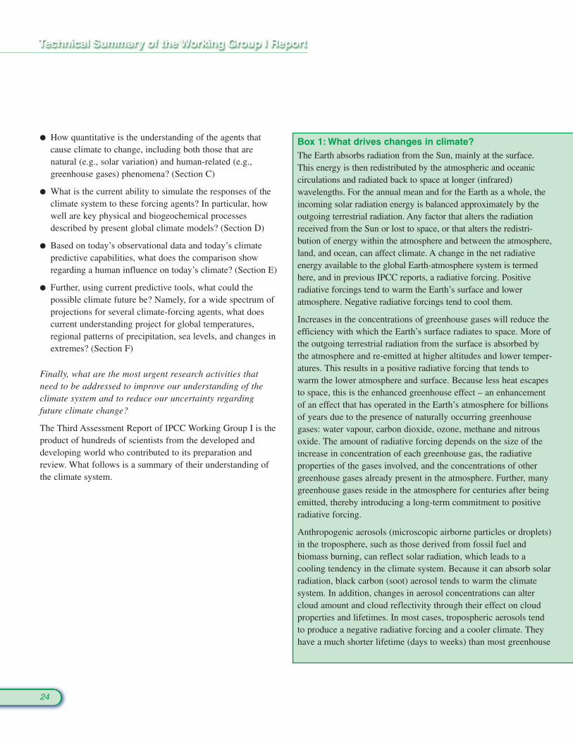
� How quantitative is the understanding of the agents thatcause climate to change, including both those that arenatural (e.g., solar variation) and human-related (e.g.,greenhouse gases) phenomena? (Section C)

� What is the current ability to simulate the responses of theclimate system to these forcing agents? In particular, howwell are key physical and biogeochemical processesdescribed by present global climate models? (Section D)

� Based on today’s observational data and today’s climatepredictive capabilities, what does the comparison showregarding a human influence on today’s climate? (Section E)

� Further, using current predictive tools, what could thepossible climate future be? Namely, for a wide spectrum ofprojections for several climate-forcing agents, what doescurrent understanding project for global temperatures,regional patterns of precipitation, sea levels, and changes inextremes? (Section F)

Finally, what are the most urgent research activities thatneed to be addressed to improve our understanding of theclimate system and to reduce our uncertainty regardingfuture climate change?

The Third Assessment Report of IPCC Working Group I is theproduct of hundreds of scientists from the developed anddeveloping world who contributed to its preparation andreview. What follows is a summary of their understanding ofthe climate system.

Box 1: What drives changes in climate?The Earth absorbs radiation from the Sun, mainly at the surface.This energy is then redistributed by the atmospheric and oceaniccirculations and radiated back to space at longer (infrared)wavelengths. For the annual mean and for the Earth as a whole, theincoming solar radiation energy is balanced approximately by theoutgoing terrestrial radiation. Any factor that alters the radiationreceived from the Sun or lost to space, or that alters the redistri-bution of energy within the atmosphere and between the atmosphere,land, and ocean, can affect climate. A change in the net radiativeenergy available to the global Earth-atmosphere system is termedhere, and in previous IPCC reports, a radiative forcing. Positiveradiative forcings tend to warm the Earth’s surface and loweratmosphere. Negative radiative forcings tend to cool them.

Increases in the concentrations of greenhouse gases will reduce theefficiency with which the Earth’s surface radiates to space. More ofthe outgoing terrestrial radiation from the surface is absorbed bythe atmosphere and re-emitted at higher altitudes and lower temper-atures. This results in a positive radiative forcing that tends towarm the lower atmosphere and surface. Because less heat escapesto space, this is the enhanced greenhouse effect – an enhancementof an effect that has operated in the Earth’s atmosphere for billionsof years due to the presence of naturally occurring greenhousegases: water vapour, carbon dioxide, ozone, methane and nitrousoxide. The amount of radiative forcing depends on the size of theincrease in concentration of each greenhouse gas, the radiativeproperties of the gases involved, and the concentrations of othergreenhouse gases already present in the atmosphere. Further, manygreenhouse gases reside in the atmosphere for centuries after beingemitted, thereby introducing a long-term commitment to positiveradiative forcing.

Anthropogenic aerosols (microscopic airborne particles or droplets)in the troposphere, such as those derived from fossil fuel andbiomass burning, can reflect solar radiation, which leads to acooling tendency in the climate system. Because it can absorb solarradiation, black carbon (soot) aerosol tends to warm the climatesystem. In addition, changes in aerosol concentrations can altercloud amount and cloud reflectivity through their effect on cloudproperties and lifetimes. In most cases, tropospheric aerosols tendto produce a negative radiative forcing and a cooler climate. Theyhave a much shorter lifetime (days to weeks) than most greenhouse

24

gases (decades to centuries), and, as a result, their concentrationsrespond much more quickly to changes in emissions.

Volcanic activity can inject large amounts of sulphur-containinggases (primarily sulphur dioxide) into the stratosphere, which aretransformed into sulphate aerosols. Individual eruptions can producea large, but transitory, negative radiative forcing, tending to cool theEarth’s surface and lower atmosphere over periods of a few years.

The Sun’s output of energy varies by small amounts (0.1%) overan 11-year cycle and, in addition, variations over longer periodsmay occur. On time-scales of tens to thousands of years, slowvariations in the Earth’s orbit, which are well understood, have ledto changes in the seasonal and latitudinal distribution of solarradiation. These changes have played an important part incontrolling the variations of climate in the distant past, such as theglacial and inter-glacial cycles.

When radiative forcing changes, the climate system responds onvarious time-scales. The longest of these are due to the large heatcapacity of the deep ocean and dynamic adjustment of the icesheets. This means that the transient response to a change (eitherpositive or negative) may last for thousands of years. Any changesin the radiative balance of the Earth, including those due to anincrease in greenhouse gases or in aerosols, will alter the globalhydrological cycle and atmospheric and oceanic circulation,thereby affecting weather patterns and regional temperatures andprecipitation.

Any human-induced changes in climate will be embedded in abackground of natural climatic variations that occur on a wholerange of time- and space-scales. Climate variability can occur as aresult of natural changes in the forcing of the climate system, forexample variations in the strength of the incoming solar radiationand changes in the concentrations of aerosols arising from volcaniceruptions. Natural climate variations can also occur in the absenceof a change in external forcing, as a result of complex interactionsbetween components of the climate system, such as the couplingbetween the atmosphere and ocean. The El Niño-SouthernOscillation (ENSO) phenomenon is an example of such natural“internal” variability on interannual time-scales. To distinguishanthropogenic climate changes from natural variations, it isnecessary to identify the anthropogenic “signal” against thebackground “noise” of natural climate variability.

B. The Observed Changes in theCl imate System

Is the Earth’s climate changing? The answer is unequivocally“Yes”. A suite of observations supports this conclusion andprovides insight about the rapidity of those changes. Thesedata are also the bedrock upon which to construct the answerto the more difficult question: “Why is it changing?”, which isaddressed in later Sections.

This Section provides an updated summary of the observationsthat delineate how the climate system has changed in the past.Many of the variables of the climate system have beenmeasured directly, i.e., the “instrumental record”. For example,widespread direct measurements of surface temperature beganaround the middle of the 19th century. Near globalobservations of other surface “weather” variables, such asprecipitation and winds, have been made for about a hundredyears. Sea level measurements have been made for over 100years in some places, but the network of tide gauges with longrecords provides only limited global coverage. Upper airobservations have been made systematically only since the late1940s. There are also long records of surface oceanicobservations made from ships since the mid-19th century andby dedicated buoys since about the late 1970s. Sub-surfaceoceanic temperature measurements with near global coverageare now available from the late 1940s. Since the late 1970s,other data from Earth-observation satellites have been used toprovide a wide range of global observations of variouscomponents of the climate system. In addition, a growing setof palaeoclimatic data, e.g., from trees, corals, sediments, andice, are giving information about the Earth’s climate ofcenturies and millennia before the present.

This Section places particular emphasis on current knowledge ofpast changes in key climate variables: temperature, precipitationand atmospheric moisture, snow cover, extent of land and seaice, sea level, patterns in atmospheric and oceanic circulation,extreme weather and climate events, and overall features of theclimate variability. The concluding part of this Section comparesthe observed trends in these various climate indicators to see if acollective picture emerges. The degree of this internalconsistency is a critical factor in assessing the level of confidencein the current understanding of the climate system.

25

B.1 Observed Changes in Temperature

Temperatures in the instrumental record forland and oceansThe global average surface temperature has increased by 0.6± 0.2°C3 since the late 19th century. It is very likely that the1990s was the warmest decade and 1998 the warmest year inthe instrumental record since 1861 (see Figure 2). The maincause of the increased estimate of global warming of 0.15°Csince the SAR is related to the record warmth of the additionalsix years (1995 to 2000) of data. A secondary reason is relatedto improved methods of estimating change. The current,slightly larger uncertainty range (±0.2°C, 95% confidenceinterval) is also more objectively based. Further, the scientificbasis for confidence in the estimates of the increase in global

temperature since the late 19th century has been strengthenedsince the SAR. This is due to the improvements derived fromseveral new studies. These include an independent test of thecorrections used for time-dependent biases in the sea surfacetemperature data and new analyses of the effect of urban “heatisland” influences on global land-temperature trends. Asindicated in Figure 2, most of the increase in global temperaturesince the late 19th century has occurred in two distinct periods:

1910 to 1945 and since 1976. The rate of increase of temperaturefor both periods is about 0.15°C/decade. Recent warming hasbeen greater over land compared to oceans; the increase in seasurface temperature over the period 1950 to 1993 is about halfthat of the mean land-surface air temperature. The high globaltemperature associated with the 1997 to 1998 El Niño eventstands out as an extreme event, even taking into account therecent rate of warming.

The regional patterns of the warming that occurred in the earlypart of the 20th century were different than those that occurredin the latter part. Figure 3 shows the regional patterns of thewarming that have occurred over the full 20th century, as wellas for three component time periods. The most recent period ofwarming (1976 to 1999) has been almost global, but the largest

increases in temperature haveoccurred over the mid- and highlatitudes of the continents in theNorthern Hemisphere. Year-roundcooling is evident in the north-western North Atlantic and thecentral North Pacific Oceans, butthe North Atlantic cooling trendhas recently reversed. The recentregional patterns of temperaturechange have been shown to berelated, in part, to various phasesof atmospheric-oceanicoscillations, such as the NorthAtlantic-Arctic Oscillation andpossibly the Pacific DecadalOscillation. Therefore, regionaltemperature trends over a fewdecades can be strongly influencedby regional variability in theclimate system and can depart

appreciably from a global average. The 1910 to 1945 warmingwas initially concentrated in the North Atlantic. By contrast, theperiod 1946 to 1975 showed significant cooling in the NorthAtlantic, as well as much of the Northern Hemisphere, andwarming in much of the Southern Hemisphere.

New analyses indicate that global ocean heat content hasincreased significantly since the late 1950s. More than halfof the increase in heat content has occurred in the upper 300 m

26

1860 1880 1900 1920 1940 1960 1980 2000Year

Dep

artu

res

in te

mpe

ratu

re (

°C)

from

the

1961

to 1

990

aver

age

GLOBAL

Data from thermometers.

-0.8

-0.4

0.0

0.4

0.8

3 Generally, temperature trends are rounded to the nearest 0.05°C per unit of time, the periods often being limited by data availability.

Figure 2: Combined annual land-surface air and sea surface temperature anomalies (°C) 1861 to 2000,

relative to 1961 to 1990. Two standard error uncertainties are shown as bars on the annual number.

[Based on Figure 2.7c]

27

(a) Annual temperature trends, 1901 to 2000 (b) Annual temperature trends, 1910 to 1945

(c) Annual temperature trends, 1946 to 1975

Trend (°C/decade)

0 0.2−0.2 0.4−0.4 0.6−0.6 0.8−0.8 1−1

(d) Annual temperature trends, 1976 to 2000

Figure 3: Annual temperature trends for the periods 1901 to 1999, 1910 to 1945, 1946 to 1975 and 1976 to 1999 respectively. Trends are represented by

the area of the circle with red representing increases, blue representing decreases, and green little or no change. Trends were calculated from annually

averaged gridded anomalies with the requirement that the calculation of annual anomalies include a minimum of 10 months of data. For the period 1901

to 1999, trends were calculated only for those grid boxes containing annual anomalies in at least 66 of the 100 years. The minimum number of years

required for the shorter time periods (1910 to 1945, 1946 to 1975, and 1976 to 1999) was 24, 20, and 16 years respectively. [Based on Figure 2.9]

of the ocean, equivalent to a rate of temperature increase inthis layer of about 0.04°C/decade.

New analyses of daily maximum and minimum land-surfacetemperatures for 1950 to 1993 continue to show that thismeasure of diurnal temperature range is decreasing verywidely, although not everywhere. On average, minimumtemperatures are increasing at about twice the rate ofmaximum temperatures (0.2 versus 0.1°C/decade).

Temperatures above the surface layer f romsatel l i te and weather bal loon recordsSurface, balloon and satellite temperature measurements showthat the troposphere and Earth’s surface have warmed andthat the stratosphere has cooled. Over the shorter time periodfor which there have been both satellite and weather balloondata (since 1979), the balloon and satellite records showsignificantly less lower-tropospheric warming than observedat the surface. Analyses of temperature trends since 1958 forthe lowest 8 km of the atmosphere and at the surface are in

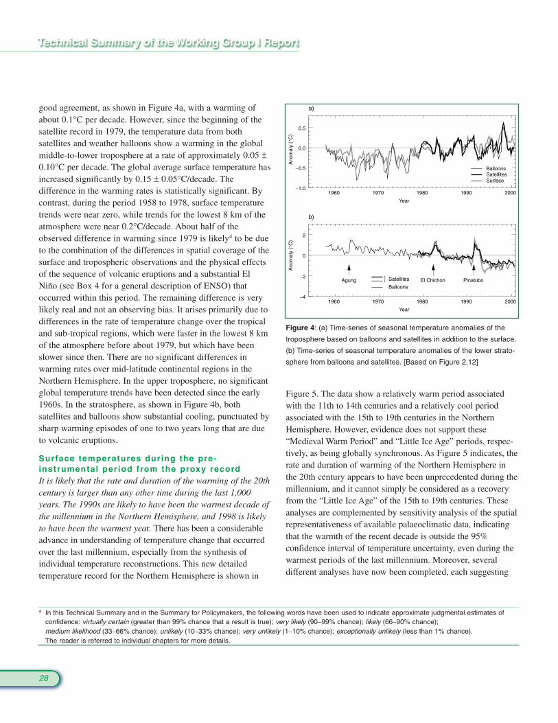
good agreement, as shown in Figure 4a, with a warming ofabout 0.1°C per decade. However, since the beginning of thesatellite record in 1979, the temperature data from bothsatellites and weather balloons show a warming in the globalmiddle-to-lower troposphere at a rate of approximately 0.05 ±0.10°C per decade. The global average surface temperature hasincreased significantly by 0.15 ± 0.05°C/decade. Thedifference in the warming rates is statistically significant. Bycontrast, during the period 1958 to 1978, surface temperaturetrends were near zero, while trends for the lowest 8 km of theatmosphere were near 0.2°C/decade. About half of theobserved difference in warming since 1979 is likely4 to be dueto the combination of the differences in spatial coverage of thesurface and tropospheric observations and the physical effectsof the sequence of volcanic eruptions and a substantial ElNiño (see Box 4 for a general description of ENSO) thatoccurred within this period. The remaining difference is verylikely real and not an observing bias. It arises primarily due todifferences in the rate of temperature change over the tropicaland sub-tropical regions, which were faster in the lowest 8 kmof the atmosphere before about 1979, but which have beenslower since then. There are no significant differences inwarming rates over mid-latitude continental regions in theNorthern Hemisphere. In the upper troposphere, no significantglobal temperature trends have been detected since the early1960s. In the stratosphere, as shown in Figure 4b, bothsatellites and balloons show substantial cooling, punctuated bysharp warming episodes of one to two years long that are dueto volcanic eruptions.

Surface temperatures during the pre-instrumental per iod from the proxy recordIt is likely that the rate and duration of the warming of the 20thcentury is larger than any other time during the last 1,000years. The 1990s are likely to have been the warmest decade ofthe millennium in the Northern Hemisphere, and 1998 is likelyto have been the warmest year. There has been a considerableadvance in understanding of temperature change that occurredover the last millennium, especially from the synthesis ofindividual temperature reconstructions. This new detailedtemperature record for the Northern Hemisphere is shown in

Figure 5. The data show a relatively warm period associatedwith the 11th to 14th centuries and a relatively cool periodassociated with the 15th to 19th centuries in the NorthernHemisphere. However, evidence does not support these“Medieval Warm Period” and “Little Ice Age” periods, respec-tively, as being globally synchronous. As Figure 5 indicates, therate and duration of warming of the Northern Hemisphere inthe 20th century appears to have been unprecedented during themillennium, and it cannot simply be considered as a recoveryfrom the “Little Ice Age” of the 15th to 19th centuries. Theseanalyses are complemented by sensitivity analysis of the spatialrepresentativeness of available palaeoclimatic data, indicatingthat the warmth of the recent decade is outside the 95%confidence interval of temperature uncertainty, even during thewarmest periods of the last millennium. Moreover, severaldifferent analyses have now been completed, each suggesting

28

Figure 4: (a) Time-series of seasonal temperature anomalies of the

troposphere based on balloons and satellites in addition to the surface.

(b) Time-series of seasonal temperature anomalies of the lower strato-

sphere from balloons and satellites. [Based on Figure 2.12]

4 In this Technical Summary and in the Summary for Policymakers, the following words have been used to indicate approximate judgmental estimates of confidence: virtually certain (greater than 99% chance that a result is true); very likely (90−99% chance); likely (66−90% chance); medium likelihood (33−66% chance); unlikely (10−33% chance); very unlikely (1−10% chance); exceptionally unlikely (less than 1% chance). The reader is referred to individual chapters for more details.

SatellitesSurface

Balloons

Satellites

Balloons

1960 1970 1980 1990 2000

Year

−1.0

−0.5

0.0

0.5

Ano

mal

y (°

C)

a)

1960 1970 1980 1990 2000

Year

−4

−2

0

2

Ano

mal

y (°

C)

b)

Agung El Chichon Pinatubo

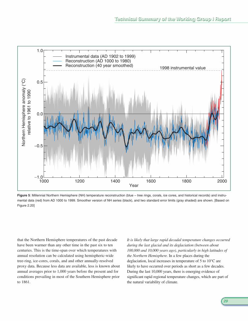
29

that the Northern Hemisphere temperatures of the past decadehave been warmer than any other time in the past six to tencenturies. This is the time-span over which temperatures withannual resolution can be calculated using hemispheric-widetree-ring, ice-cores, corals, and and other annually-resolvedproxy data. Because less data are available, less is known aboutannual averages prior to 1,000 years before the present and forconditions prevailing in most of the Southern Hemisphere priorto 1861.

It is likely that large rapid decadal temperature changes occurredduring the last glacial and its deglaciation (between about100,000 and 10,000 years ago), particularly in high latitudes ofthe Northern Hemisphere. In a few places during thedeglaciation, local increases in temperature of 5 to 10°C arelikely to have occurred over periods as short as a few decades.During the last 10,000 years, there is emerging evidence ofsignificant rapid regional temperature changes, which are part ofthe natural variability of climate.

1000 1200 1400 1600 1800 2000Year

−1.0

−0.5

0.0

0.5

1.0

rel

ativ

e to

196

1 to

199

0N

orth

ern

Hem

isph

ere

anom

aly

(°C

)

1998 instrumental value

Instrumental data (AD 1902 to 1999)Reconstruction (AD 1000 to 1980)Reconstruction (40 year smoothed)

Figure 5: Millennial Northern Hemisphere (NH) temperature reconstruction (blue – tree rings, corals, ice cores, and historical records) and instru-

mental data (red) from AD 1000 to 1999. Smoother version of NH series (black), and two standard error limits (gray shaded) are shown. [Based on

Figure 2.20]

B.3 Observed Changes in Snow Cover andLand- and Sea- Ice Extent

Decreasing snow cover and land-ice extent continue to bepositively correlated with increasing land-surface temper-atures. Satellite data show that there are very likely to havebeen decreases of about 10% in the extent of snow coversince the late 1960s. There is a highly significant correlationbetween increases in Northern Hemisphere land temper-atures and the decreases. There is now ample evidence tosupport a major retreat of alpine and continental glaciers inresponse to 20th century warming. In a few maritimeregions, increases in precipitation due to regionalatmospheric circulation changes have overshadowedincreases in temperature in the past two decades, andglaciers have re-advanced. Over the past 100 to 150 years,ground-based observations show that there is very likely tohave been a reduction of about two weeks in the annualduration of lake and river ice in the mid- to high latitudes ofthe Northern Hemisphere.

Northern Hemisphere sea-ice amounts are decreasing, butno significant trends in Antarctic sea-ice extent areapparent. A retreat of sea-ice extent in the Arctic spring andsummer of 10 to 15% since the 1950s is consistent with anincrease in spring temperatures and, to a lesser extent,summer temperatures in the high latitudes. There is littleindication of reduced Arctic sea-ice extent during winterwhen temperatures have increased in the surrounding region.By contrast, there is no readily apparent relationshipbetween decadal changes of Antarctic temperatures and sea-ice extent since 1973. After an initial decrease in themid-1970s, Antarctic sea-ice extent has remained stable, oreven slightly increased.

New data indicate that there likely has been an approxi-mately 40% decline in Arctic sea-ice thickness in latesummer to early autumn between the period of 1958 to 1976and the mid-1990s, and a substantially smaller decline inwinter. The relatively short record length and incompletesampling limit the interpretation of these data. Interannualvariability and inter-decadal variability could be influencingthese changes.

B.2 Observed Changes in Precipi tat ion andAtmospheric Moisture

Since the time of the SAR, annual land precipitation hascontinued to increase in the middle and high latitudes of theNorthern Hemisphere (very likely to be 0.5 to 1%/decade), exceptover Eastern Asia. Over the sub-tropics (10°N to 30°N), land-surface rainfall has decreased on average (likely to be about0.3%/decade), although this has shown signs of recovery in recentyears. Tropical land-surface precipitation measurements indicatethat precipitation likely has increased by about 0.2 to 0.3%/decade over the 20th century, but increases are not evident overthe past few decades and the amount of tropical land (versusocean) area for the latitudes 10°N to 10°S is relatively small.Nonetheless, direct measurements of precipitation and modelreanalyses of inferred precipitation indicate that rainfall has alsoincreased over large parts of the tropical oceans. Where and whenavailable, changes in annual streamflow often relate well tochanges in total precipitation. The increases in precipitation overNorthern Hemisphere mid- and high latitude land areas have astrong correlation to long-term increases in total cloud amount. Incontrast to the Northern Hemisphere, no comparable systematicchanges in precipitation have been detected in broad latitudinalaverages over the Southern Hemisphere.

It is likely that total atmospheric water vapour has increasedseveral per cent per decade over many regions of the NorthernHemisphere. Changes in water vapour over approximately thepast 25 years have been analysed for selected regions using in situsurface observations, as well as lower-tropospheric measurementsfrom satellites and weather balloons. A pattern of overall surfaceand lower-tropospheric water vapour increases over the past fewdecades is emerging from the most reliable data sets, althoughthere are likely to be time-dependent biases in these data andregional variations in the trends. Water vapour in the lower strato-sphere is also likely to have increased by about 10% per decadesince the beginning of the observational record (1980).

Changes in total cloud amounts over Northern Hemisphere mid- and high latitude continental regions indicate a likelyincrease in cloud cover of about 2% since the beginning of the20th century, which has now been shown to be positivelycorrelated with decreases in the diurnal temperature range.Similar changes have been shown over Australia, the onlySouthern Hemisphere continent where such an analysis has beencompleted. Changes in total cloud amount are uncertain both oversub-tropical and tropical land areas, as well as over the oceans.

30

31

B.4 Observed Changes in Sea Level

Changes during the instrumental recordBased on tide gauge data, the rate of global mean sea level riseduring the 20th century is in the range 1.0 to 2.0 mm/yr, with acentral value of 1.5 mm/yr (the central value should not beinterpreted as a best estimate). (See Box 2 for the factors thatinfluence sea level.) As Figure 6 indicates, the longest instrumentalrecords (two or three centuries at most) of local sea level comefrom tide gauges. Based on the very few long tide-gauge records,the average rate of sea level rise has been larger during the 20thcentury than during the 19th century. No significant acceleration

in the rate of sea level rise during the 20th century has beendetected. This is not inconsistent with model results due to thepossibility of compensating factors and the limited data.

Changes during the pre- instrumental recordSince the last glacial maximum about 20,000 years ago, thesea level in locations far from present and former ice sheetshas risen by over 120 m as a result of loss of mass from theseice sheets. Vertical land movements, both upward anddownward, are still occurring in response to these largetransfers of mass from ice sheets to oceans. The most rapidrise in global sea level was between 15,000 and 6,000 years

Box 2: What causes sea level tochange?The level of the sea at the shoreline isdetermined by many factors in theglobal environment that operate on agreat range of time-scales, from hours(tidal) to millions of years (oceanbasin changes due to tectonics andsedimentation). On the time-scale ofdecades to centuries, some of thelargest influences on the averagelevels of the sea are linked to climateand climate change processes.

Firstly, as ocean water warms, itexpands. On the basis of observationsof ocean temperatures and modelresults, thermal expansion is believedto be one of the major contributors tohistorical sea level changes. Further,thermal expansion is expected tocontribute the largest component tosea level rise over the next hundredyears. Deep ocean temperatureschange only slowly; therefore, thermalexpansion would continue for manycenturies even if the atmosphericconcentrations of greenhouse gaseswere to stabilise.

The amount of warming and the depthof water affected vary with location.In addition, warmer water expands

more than colder water for a givenchange in temperature. Thegeographical distribution of sea levelchange results from the geographicalvariation of thermal expansion,changes in salinity, winds, and oceancirculation. The range of regionalvariation is substantial compared withthe global average sea level rise.

Sea level also changes when the massof water in the ocean increases ordecreases. This occurs when oceanwater is exchanged with the waterstored on land. The major land store isthe water frozen in glaciers or icesheets. Indeed, the main reason for thelower sea level during the last glacialperiod was the amount of water storedin the large extension of the ice sheetson the continents of the NorthernHemisphere. After thermal expansion,the melting of mountain glaciers andice caps is expected to make thelargest contribution to the rise of sealevel over the next hundred years.These glaciers and ice caps make uponly a few per cent of the world’sland-ice area, but they are moresensitive to climate change than thelarger ice sheets in Greenland andAntarctica, because the ice sheets arein colder climates with low precipitation

and low melting rates. Consequently,the large ice sheets are expected tomake only a small net contribution tosea level change in the comingdecades.

Sea level is also influenced byprocesses that are not explicitlyrelated to climate change. Terrestrialwater storage (and hence, sea level)can be altered by extraction of groundwater, building of reservoirs, changesin surface runoff, and seepage intodeep aquifers from reservoirs andirrigation. These factors may beoffsetting a significant fraction of theexpected acceleration in sea level risefrom thermal expansion and glacialmelting. In addition, coastalsubsidence in river delta regions canalso influence local sea level. Verticalland movements caused by naturalgeological processes, such as slowmovements in the Earth’s mantle andtectonic displacements of the crust,can have effects on local sea level thatare comparable to climate-relatedimpacts. Lastly, on seasonal,interannual, and decadal time-scales,sea level responds to changes inatmospheric and ocean dynamics, withthe most striking example occurringduring El Niño events.

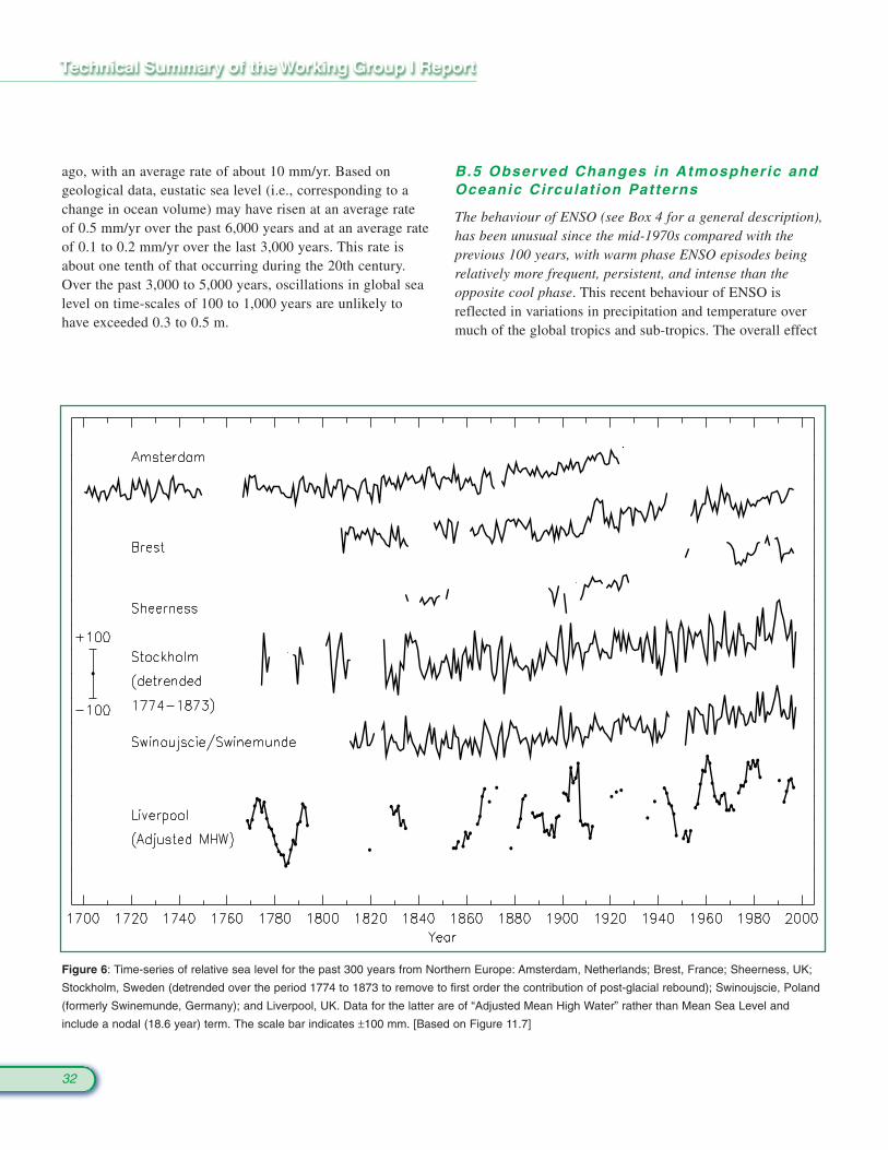
32

Figure 6: Time-series of relative sea level for the past 300 years from Northern Europe: Amsterdam, Netherlands; Brest, France; Sheerness, UK;

Stockholm, Sweden (detrended over the period 1774 to 1873 to remove to first order the contribution of post-glacial rebound); Swinoujscie, Poland

(formerly Swinemunde, Germany); and Liverpool, UK. Data for the latter are of “Adjusted Mean High Water” rather than Mean Sea Level and

include a nodal (18.6 year) term. The scale bar indicates ±100 mm. [Based on Figure 11.7]

ago, with an average rate of about 10 mm/yr. Based ongeological data, eustatic sea level (i.e., corresponding to achange in ocean volume) may have risen at an average rateof 0.5 mm/yr over the past 6,000 years and at an average rateof 0.1 to 0.2 mm/yr over the last 3,000 years. This rate isabout one tenth of that occurring during the 20th century.Over the past 3,000 to 5,000 years, oscillations in global sealevel on time-scales of 100 to 1,000 years are unlikely tohave exceeded 0.3 to 0.5 m.

B.5 Observed Changes in Atmospheric andOceanic Circulat ion Patterns

The behaviour of ENSO (see Box 4 for a general description),has been unusual since the mid-1970s compared with theprevious 100 years, with warm phase ENSO episodes beingrelatively more frequent, persistent, and intense than theopposite cool phase. This recent behaviour of ENSO isreflected in variations in precipitation and temperature overmuch of the global tropics and sub-tropics. The overall effect

33

is likely to have been a small contribution to the increase inglobal temperatures during the last few decades. The Inter-decadal Pacific Oscillation and the Pacific DecadalOscillation are associated with decadal to multidecadalclimate variability over the Pacific basin. It is likely that theseoscillations modulate ENSO-related climate variability.

Other important circulation features that affect the climatein large regions of the globe are being characterised. TheNorth Atlantic Oscillation (NAO) is linked to the strength ofthe westerlies over the Atlantic and extra-tropical Eurasia.During winter the NAO displays irregular oscillations oninterannual to multi-decadal time-scales. Since the 1970s,the winter NAO has often been in a phase that contributes tostronger westerlies, which correlate with cold seasonwarming over Eurasia. New evidence indicates that the NAOand changes in Arctic sea ice are likely to be closelycoupled. The NAO is now believed to be part of a widerscale atmospheric Arctic Oscillation that affects much of theextratropical Northern Hemisphere. A similar AntarcticOscillation has been in an enhanced positive phase duringthe last 15 years, with stronger westerlies over the SouthernOceans.

B.6 Observed Changes in Cl imateVariabi l i ty and Extreme Weather andClimate Events

New analyses show that in regions where total precipitationhas increased, it is very likely that there have been even morepronounced increases in heavy and extreme precipitationevents. The converse is also true. In some regions, however,heavy and extreme events (i.e., defined to be within theupper or lower ten percentiles) have increased despite thefact that total precipitation has decreased or remainedconstant. This is attributed to a decrease in the frequency ofprecipitation events. Overall, it is likely that for many mid-and high latitude areas, primarily in the NorthernHemisphere, statistically significant increases have occurredin the proportion of total annual precipitation derived fromheavy and extreme precipitation events; it is likely that therehas been a 2 to 4% increase in the frequency of heavyprecipitation events over the latter half of the 20th century.Over the 20th century (1900 to 1995), there were relativelysmall increases in global land areas experiencing severedrought or severe wetness. In some regions, such as parts of

Asia and Africa, the frequency and intensity of drought havebeen observed to increase in recent decades. In manyregions, these changes are dominated by inter-decadal andmulti-decadal climate variability, such as the shift in ENSOtowards more warm events. In many regions, inter-dailytemperature variability has decreased, and increases in thedaily minimum temperature are lengthening the freeze-freeperiod in most mid- and high latitude regions. Since 1950 itis very likely that there has been a significant reduction inthe frequency of much-below-normal seasonal mean temper-atures across much of the globe, but there has been a smallerincrease in the frequency of much-above-normal seasonaltemperatures.

There is no compelling evidence to indicate that the characteristics of tropical and extratropical storms havechanged. Changes in tropical storm intensity and frequencyare dominated by interdecadal to multidecadal variations,which may be substantial, e.g., in the tropical North Atlantic.Owing to incomplete data and limited and conflictinganalyses, it is uncertain as to whether there have been anylong-term and large-scale increases in the intensity andfrequency of extra-tropical cyclones in the NorthernHemisphere. Regional increases have been identified in theNorth Pacific, parts of North America, and Europe over thepast several decades. In the Southern Hemisphere, feweranalyses have been completed, but they suggest a decrease inextra-tropical cyclone activity since the 1970s. Recentanalyses of changes in severe local weather (e.g., tornadoes,thunderstorm days, and hail) in a few selected regions do notprovide compelling evidence to suggest long-term changes.In general, trends in severe weather events are notoriouslydifficult to detect because of their relatively rare occurrenceand large spatial variability.

B.7 The Collective Picture: A Warming Worldand Other Changes in the Climate System

As summarised above, a suite of climate changes is now well-documented, particularly over the recent decades tocentury time period, with its growing set of directmeasurements. Figure 7 illustrates these trends in temperatureindicators (Figure 7a) and hydrological and storm-relatedindicators (Figure 7b), as well as also providing an indicationof certainty about the changes.

34

Taken together, these trends illustrate a collective pictureof a warming world:� Surface temperature measurements over the land and

oceans (with two separate estimates over the latter) havebeen measured and adjusted independently. All data setsshow quite similar upward trends globally, with two majorwarming periods globally: 1910 to 1945 and since 1976.There is an emerging tendency for global land-surface airtemperatures to warm faster than the global ocean-surfacetemperatures.

� Weather balloon measurements show that lower-tropospherictemperatures have been increasing since 1958, though onlyslightly since 1979. Since 1979, satellite data are availableand show similar trends to balloon data.

� The decrease in the continental diurnal temperature rangecoincides with increases in cloud amount, precipitation, andincreases in total water vapour.

� The nearly worldwide decrease in mountain glacier extentand ice mass is consistent with worldwide surfacetemperature increases. A few recent exceptions in coastalregions are consistent with atmospheric circulationvariations and related precipitation increases.

� The decreases in snow cover and the shortening seasons oflake and river ice relate well to increases in NorthernHemispheric land-surface temperatures.

� The systematic decrease in spring and summer sea-iceextent and thickness in the Arctic is consistent withincreases in temperature over most of the adjacent land andocean.

� Ocean heat content has increased, and global average sealevel has risen.

� The increases in total tropospheric water vapour in the last25 years are qualitatively consistent with increases intropospheric temperatures and an enhanced hydrologiccycle, resulting in more extreme and heavier precipitationevents in many areas with increasing precipitation, e.g.,middle and high latitudes of the Northern Hemisphere.

Some important aspects of climate appear not to havechanged.� A few areas of the globe have not warmed in recent

decades, mainly over some parts of the Southern Hemisphereoceans and parts of Antarctica.

� No significant trends in Antarctic sea-ice extent are apparentover the period of systematic satellite measurements (since1978).

� Based on limited data, the observed variations in theintensity and frequency of tropical and extra-tropicalcyclones and severe local storms show no clear trends in thelast half of the 20th century, although multi-decadal fluctu-ations are sometimes apparent.

The variations and trends in the examined indicators implythat it is virtually certain that there has been a generallyincreasing trend in global surface temperature over the 20thcentury, although short-term and regional deviations from thistrend occur.

35

LOWER STRATOSPHERE

TROPOSPHERE

NEAR-SURFACE

*** sea surface temperature:0.4 to 0.8oC increase sincethe late 19th century.

0.0 to 0.2oC increase since 1979 - satellites & balloons

** lower stratosphere: 0.5 to 2.5 oC decrease since 1979

*** land air temperatures: 0.4 to 0.8oC

** N.H. Spring snow cover extent: since 1987, 10% below 1966-86 mean

*** massive retreat of mountain glaciers during 20th century

* land night time air temperature increasing at twice the rate of daytime temperatures since 1950

* Arctic sea ice: summer thickness decrease of 40%and 10 to 15% decrease in extent during spring and summer since 1950s

(a) Temperature Indicators

** marine air temperature: 0.4 to 0.7oCincrease since late-19th century

* 0.2 to 0.4oC increase since ~1960

lake and river ice retreat at mid and high since the late 19th century (2 week

? Antarctic sea ice: no significant change since 1978

1990s warmest decade of the millennium and 1998 warmest year for at least the N.H.

O C E A NL A N DO C E A N

**

*

* global ocean (to 300m depth) heat content increase since 1950s equal to 0.04 C / decadeo

**latitudesdecrease in ice duration)

Virtually certain (probability > 99%)Very likely (probability > 90% but < 99%)Likely (probability > 66% but < 90%)Medium likelihood (probability > 33% but < 66%)

******?

Likelihood:

Low- to Mid-

Upper * Little or no change since 1979

increase since late 19th century

_ _

_

Figure 7a: Schematic of observed variations of

the temperature indicators. [Based on Figure

2.39a]

Figure 7b: Schematic of observed variations of

the hydrological and storm-related indicators.

[Based on Figure 2.39b]LOWER STRATOSPHERE

TROPOSPHERE

NEAR-SURFACE

** 5 to10% increase in N. Hemisphere mid-to-high latitude precipitation since 1900,

of it due to heavy / extreme events

?

troposphere: *many regions with increases since about 1960

* widespread significant increases in surface water vapour in the

N. Hemisphere, 1975 to 1995

* 2% increase in total cloud amount over land during the 20th century

2% increase in total cloud amount over the ocean since 1952

** no widespread changes in tropical storm frequency / intensity during the 20th century

no consistent 20th centurychange in extra-tropicalstorm frequency / intensity

❄❄

❄❄

❄❄

❄❄

❄

❄

O C E A NL A N DO C E A N

Virtually certain (probability > 99%)Very likely (probability > 90% but < 99%)Likely (probability > 66% but < 90%)Medium likelihood (probability > 33% but < 66%)

******?

20% water vapour increase since 1980 (above 18 km)

Water vapour

upper troposphere: *no significant global trends since 1980;

*

no systematic large-scalechange in tornadoes, thunder-days, hail

?

?

Likelihood:

20th century land surface rainfall

* 2 to 3% decrease in sub-tropics

* 2 to 3% increase in tropics

15% increase in tropics (10°N to 10°S)

_ _

_

with much

(b) Hydrological and Storm related Indicators

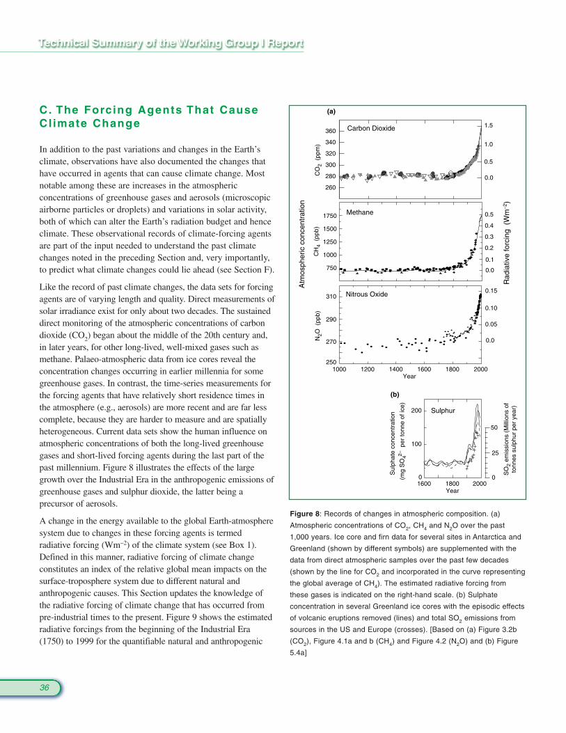
36

CO

2 (

ppm

)

260

280

300

320

340

360

1000 1200 1400 1600 1800 2000

CH

4 (

ppb)

1250

1000

750

1500

1750

N2O

(pp

b)

310

290

270

250

0.0

0.5

1.0

1.5

0.5

0.4

0.3

0.2

0.1

0.0

0.15

0.10

0.05

0.0

Carbon Dioxide

Methane

Nitrous OxideA

tmos

pher

ic c

once

ntra

tion

Rad

iativ

e fo

rcin

g (

Wm

−2)

1600 1800

200

100

0(mg

SO

42– p

er to

nne

of ic

e)

Sulphur

Sul

phat

e co

ncen

trat

ion

Year

Year2000

50

25

0 SO

2 em

issi

ons

(Mill

ions

of

tonn

es s

ulph

ur p

er y

ear)

(b)

(a)

Figure 8: Records of changes in atmospheric composition. (a)

Atmospheric concentrations of CO2, CH4 and N2O over the past

1,000 years. Ice core and firn data for several sites in Antarctica and

Greenland (shown by different symbols) are supplemented with the

data from direct atmospheric samples over the past few decades

(shown by the line for CO2 and incorporated in the curve representing

the global average of CH4). The estimated radiative forcing from

these gases is indicated on the right-hand scale. (b) Sulphate

concentration in several Greenland ice cores with the episodic effects

of volcanic eruptions removed (lines) and total SO2 emissions from

sources in the US and Europe (crosses). [Based on (a) Figure 3.2b

(CO2), Figure 4.1a and b (CH4) and Figure 4.2 (N2O) and (b) Figure

5.4a]

C. The Forcing Agents That CauseCl imate Change

In addition to the past variations and changes in the Earth’sclimate, observations have also documented the changes thathave occurred in agents that can cause climate change. Mostnotable among these are increases in the atmospheric concentrations of greenhouse gases and aerosols (microscopicairborne particles or droplets) and variations in solar activity,both of which can alter the Earth’s radiation budget and henceclimate. These observational records of climate-forcing agentsare part of the input needed to understand the past climatechanges noted in the preceding Section and, very importantly,to predict what climate changes could lie ahead (see Section F).

Like the record of past climate changes, the data sets for forcingagents are of varying length and quality. Direct measurements ofsolar irradiance exist for only about two decades. The sustaineddirect monitoring of the atmospheric concentrations of carbondioxide (CO2) began about the middle of the 20th century and,in later years, for other long-lived, well-mixed gases such asmethane. Palaeo-atmospheric data from ice cores reveal theconcentration changes occurring in earlier millennia for somegreenhouse gases. In contrast, the time-series measurements forthe forcing agents that have relatively short residence times inthe atmosphere (e.g., aerosols) are more recent and are far lesscomplete, because they are harder to measure and are spatiallyheterogeneous. Current data sets show the human influence onatmospheric concentrations of both the long-lived greenhousegases and short-lived forcing agents during the last part of thepast millennium. Figure 8 illustrates the effects of the largegrowth over the Industrial Era in the anthropogenic emissions ofgreenhouse gases and sulphur dioxide, the latter being aprecursor of aerosols.

A change in the energy available to the global Earth-atmospheresystem due to changes in these forcing agents is termedradiative forcing (Wm−2) of the climate system (see Box 1).Defined in this manner, radiative forcing of climate changeconstitutes an index of the relative global mean impacts on thesurface-troposphere system due to different natural and anthropogenic causes. This Section updates the knowledge ofthe radiative forcing of climate change that has occurred frompre-industrial times to the present. Figure 9 shows the estimatedradiative forcings from the beginning of the Industrial Era(1750) to 1999 for the quantifiable natural and anthropogenic

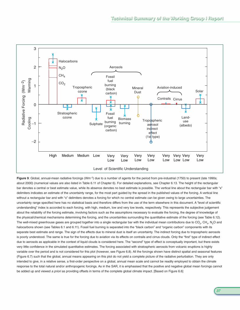
37

−2

−1

0

1

2

3

Rad

iativ

e F

orci

ng (

Wm

−2)

CO2

CH4

N2O

Halocarbons

(1st type)

Level of Scientific Understanding

Coo

ling

War

min

g

High Medium Medium Low VeryLow

VeryLow

VeryLow

VeryLow

VeryLow

VeryLow

VeryLow

Stratosphericozone

Troposphericozone

Sulphate

Fossilfuel

burning(black

carbon)

Fossilfuel

burning(organic carbon)

Biomassburning

Contrails

SolarMineral

Dust

Tropospheric aerosolindirect effect

Land-use

(albedo)

Aviation-induced

Cirrus

VeryLow

Aerosols

Figure 9: Global, annual-mean radiative forcings (Wm−2) due to a number of agents for the period from pre-industrial (1750) to present (late 1990s;

about 2000) (numerical values are also listed in Table 6.11 of Chapter 6). For detailed explanations, see Chapter 6.13. The height of the rectangular

bar denotes a central or best estimate value, while its absence denotes no best estimate is possible. The vertical line about the rectangular bar with “x”

delimiters indicates an estimate of the uncertainty range, for the most part guided by the spread in the published values of the forcing. A vertical line

without a rectangular bar and with “o” delimiters denotes a forcing for which no central estimate can be given owing to large uncertainties. The

uncertainty range specified here has no statistical basis and therefore differs from the use of the term elsewhere in this document. A “level of scientific

understanding” index is accorded to each forcing, with high, medium, low and very low levels, respectively. This represents the subjective judgement

about the reliability of the forcing estimate, involving factors such as the assumptions necessary to evaluate the forcing, the degree of knowledge of

the physical/chemical mechanisms determining the forcing, and the uncertainties surrounding the quantitative estimate of the forcing (see Table 6.12).

The well-mixed greenhouse gases are grouped together into a single rectangular bar with the individual mean contributions due to CO2, CH4, N2O and

halocarbons shown (see Tables 6.1 and 6.11). Fossil fuel burning is separated into the “black carbon” and “organic carbon” components with its

separate best estimate and range. The sign of the effects due to mineral dust is itself an uncertainty. The indirect forcing due to tropospheric aerosols

is poorly understood. The same is true for the forcing due to aviation via its effects on contrails and cirrus clouds. Only the “first” type of indirect effect

due to aerosols as applicable in the context of liquid clouds is considered here. The “second” type of effect is conceptually important, but there exists

very little confidence in the simulated quantitative estimates. The forcing associated with stratospheric aerosols from volcanic eruptions is highly

variable over the period and is not considered for this plot (however, see Figure 6.8). All the forcings shown have distinct spatial and seasonal features

(Figure 6.7) such that the global, annual means appearing on this plot do not yield a complete picture of the radiative perturbation. They are only

intended to give, in a relative sense, a first-order perspective on a global, annual mean scale and cannot be readily employed to obtain the climate

response to the total natural and/or anthropogenic forcings. As in the SAR, it is emphasised that the positive and negative global mean forcings cannot

be added up and viewed a priori as providing offsets in terms of the complete global climate impact. [Based on Figure 6.6]

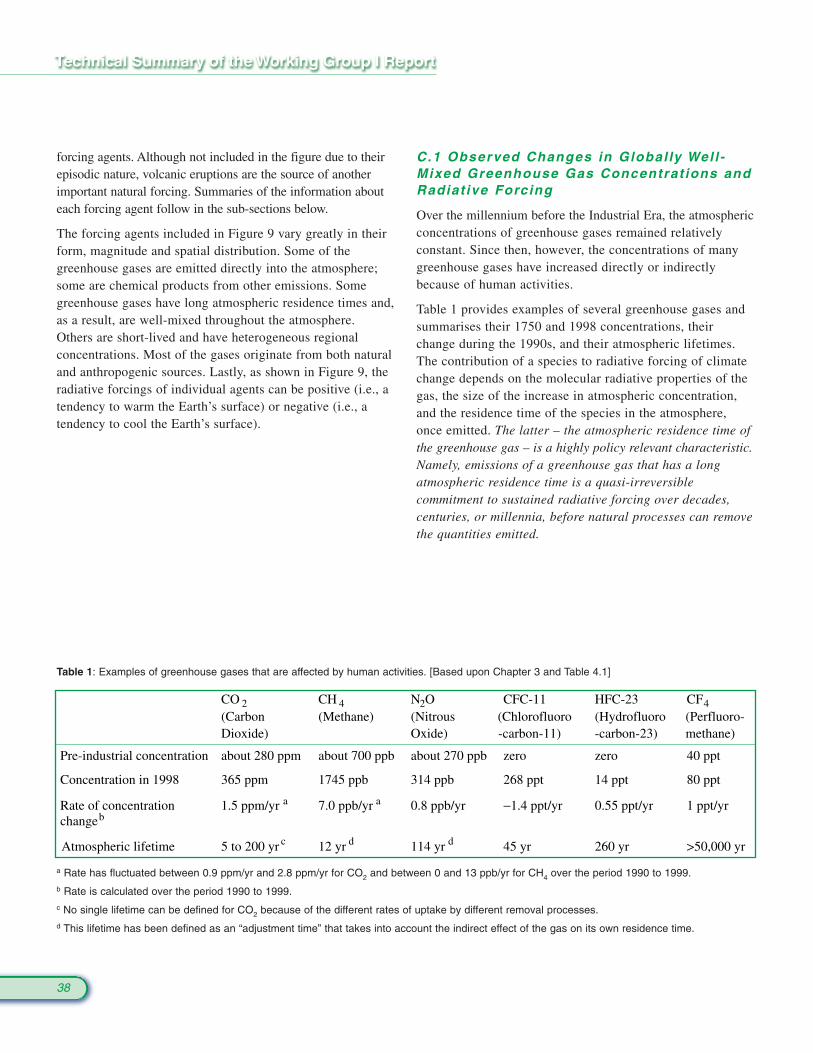
C.1 Observed Changes in Global ly Wel l -Mixed Greenhouse Gas Concentrat ions andRadiat ive Forcing

Over the millennium before the Industrial Era, the atmosphericconcentrations of greenhouse gases remained relativelyconstant. Since then, however, the concentrations of manygreenhouse gases have increased directly or indirectlybecause of human activities.

Table 1 provides examples of several greenhouse gases andsummarises their 1750 and 1998 concentrations, theirchange during the 1990s, and their atmospheric lifetimes.The contribution of a species to radiative forcing of climatechange depends on the molecular radiative properties of thegas, the size of the increase in atmospheric concentration,and the residence time of the species in the atmosphere,once emitted. The latter – the atmospheric residence time ofthe greenhouse gas – is a highly policy relevant characteristic.Namely, emissions of a greenhouse gas that has a longatmospheric residence time is a quasi-irreversiblecommitment to sustained radiative forcing over decades,centuries, or millennia, before natural processes can removethe quantities emitted.

forcing agents. Although not included in the figure due to theirepisodic nature, volcanic eruptions are the source of anotherimportant natural forcing. Summaries of the information abouteach forcing agent follow in the sub-sections below.

The forcing agents included in Figure 9 vary greatly in theirform, magnitude and spatial distribution. Some of thegreenhouse gases are emitted directly into the atmosphere;some are chemical products from other emissions. Somegreenhouse gases have long atmospheric residence times and,as a result, are well-mixed throughout the atmosphere.Others are short-lived and have heterogeneous regional concentrations. Most of the gases originate from both naturaland anthropogenic sources. Lastly, as shown in Figure 9, theradiative forcings of individual agents can be positive (i.e., atendency to warm the Earth’s surface) or negative (i.e., atendency to cool the Earth’s surface).

38

Table 1: Examples of greenhouse gases that are affected by human activities. [Based upon Chapter 3 and Table 4.1]

CO 2(CarbonDioxide)

CH 4(Methane)

N2O(NitrousOxide)

CFC-11(Chlorofluoro-carbon-11)

HFC-23(Hydrofluoro-carbon-23)

CF4(Perfluoro-methane)

Pre-industrial concentration about 280 ppm about 700 ppb about 270 ppb zero zero 40 ppt

Concentration in 1998 365 ppm 1745 ppb 314 ppb 268 ppt 14 ppt 80 ppt

Rate of concentrationchange b

1.5 ppm/yr a 7.0 ppb/yr a 0.8 ppb/yr −1.4 ppt/yr 0.55 ppt/yr 1 ppt/yr

Atmospheric lifetime 5 to 200 yr c 12 yr d 114 yr d 45 yr 260 yr >50,000 yr

a Rate has fluctuated between 0.9 ppm/yr and 2.8 ppm/yr for CO2 and between 0 and 13 ppb/yr for CH4 over the period 1990 to 1999.b Rate is calculated over the period 1990 to 1999.c No single lifetime can be defined for CO2 because of the different rates of uptake by different removal processes.d This lifetime has been defined as an “adjustment time” that takes into account the indirect effect of the gas on its own residence time.

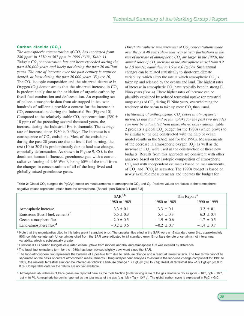
Carbon dioxide (CO2)The atmospheric concentration of CO2 has increased from280 ppm5 in 1750 to 367 ppm in 1999 (31%, Table 1).Today’s CO2 concentration has not been exceeded during thepast 420,000 years and likely not during the past 20 millionyears. The rate of increase over the past century is unprece-dented, at least during the past 20,000 years (Figure 10).The CO2 isotopic composition and the observed decrease inOxygen (O2) demonstrates that the observed increase in CO2is predominately due to the oxidation of organic carbon byfossil-fuel combustion and deforestation. An expanding setof palaeo-atmospheric data from air trapped in ice overhundreds of millennia provide a context for the increase inCO2 concentrations during the Industrial Era (Figure 10).Compared to the relatively stable CO2 concentrations (280 ±10 ppm) of the preceding several thousand years, theincrease during the Industrial Era is dramatic. The averagerate of increase since 1980 is 0.4%/yr. The increase is aconsequence of CO2 emissions. Most of the emissionsduring the past 20 years are due to fossil fuel burning, therest (10 to 30%) is predominantly due to land-use change,especially deforestation. As shown in Figure 9, CO2 is thedominant human-influenced greenhouse gas, with a currentradiative forcing of 1.46 Wm−2, being 60% of the total fromthe changes in concentrations of all of the long-lived andglobally mixed greenhouse gases.

Direct atmospheric measurements of CO2 concentrations madeover the past 40 years show that year to year fluctuations in therate of increase of atmospheric CO2 are large. In the 1990s, theannual rates of CO2 increase in the atmosphere varied from 0.9to 2.8 ppm/yr, equivalent to 1.9 to 6.0 PgC/yr. Such annualchanges can be related statistically to short-term climatevariability, which alters the rate at which atmospheric CO2 istaken up and released by the oceans and land. The highest ratesof increase in atmospheric CO2 have typically been in strong ElNiño years (Box 4). These higher rates of increase can beplausibly explained by reduced terrestrial uptake (or terrestrialoutgassing) of CO2 during El Niño years, overwhelming thetendency of the ocean to take up more CO2 than usual.

Partitioning of anthropogenic CO2 between atmosphericincreases and land and ocean uptake for the past two decadescan now be calculated from atmospheric observations. Table2 presents a global CO2 budget for the 1980s (which proves tobe similar to the one constructed with the help of oceanmodel results in the SAR) and for the 1990s. Measurementsof the decrease in atmospheric oxygen (O2) as well as theincrease in CO2 were used in the construction of these newbudgets. Results from this approach are consistent with otheranalyses based on the isotopic composition of atmosphericCO2 and with independent estimates based on measurementsof CO2 and 13CO2 in seawater. The 1990s budget is based onnewly available measurements and updates the budget for

39

SARa,b This Report a

1980 to 1989 1980 to 1989 1990 to 1999

Atmospheric increase 3.3 ± 0.1 3.3 ± 0.1 3.2 ± 0.1Emissions (fossil fuel, cement) c 5.5 ± 0.3 5.4 ± 0.3 6.3 ± 0.4Ocean-atmosphere flux − 2.0 ± 0.5 −1.9 ± 0.6 −1.7 ± 0.5Land-atmosphere flux d − 0.2 ± 0.6 −0.2 ± 0.7 −1.4 ± 0.7

Table 2: Global CO2 budgets (in PgC/yr) based on measurements of atmospheric CO2 and O2. Positive values are fluxes to the atmosphere;

negative values represent uptake from the atmosphere. [Based upon Tables 3.1 and 3.3]

a Note that the uncertainties cited in this table are ±1 standard error. The uncertainties cited in the SAR were ±1.6 standard error (i.e., approximately90% confidence interval). Uncertainties cited from the SAR were adjusted to ±1 standard error. Error bars denote uncertainty, not interannualvariability, which is substantially greater.

b Previous IPCC carbon budgets calculated ocean uptake from models and the land-atmosphere flux was inferred by difference.c The fossil fuel emissions term for the 1980s has been revised slightly downward since the SAR.d The land-atmosphere flux represents the balance of a positive term due to land-use change and a residual terrestrial sink. The two terms cannot be

separated on the basis of current atmospheric measurements. Using independent analyses to estimate the land-use change component for 1980 to1989, the residual terrestrial sink can be inferred as follows: Land-use change 1.7 PgC/yr (0.6 to 2.5); Residual terrestrial sink −1.9 PgC/yr (−3.8 to0.3). Comparable data for the 1990s are not yet available.

5 Atmospheric abundances of trace gases are reported here as the mole fraction (molar mixing ratio) of the gas relative to dry air (ppm = 10−6, ppb = 10−9,

ppt = 10−12). Atmospheric burden is reported as the total mass of the gas (e.g., Mt = Tg = 1012 g). The global carbon cycle is expressed in PgC = GtC.

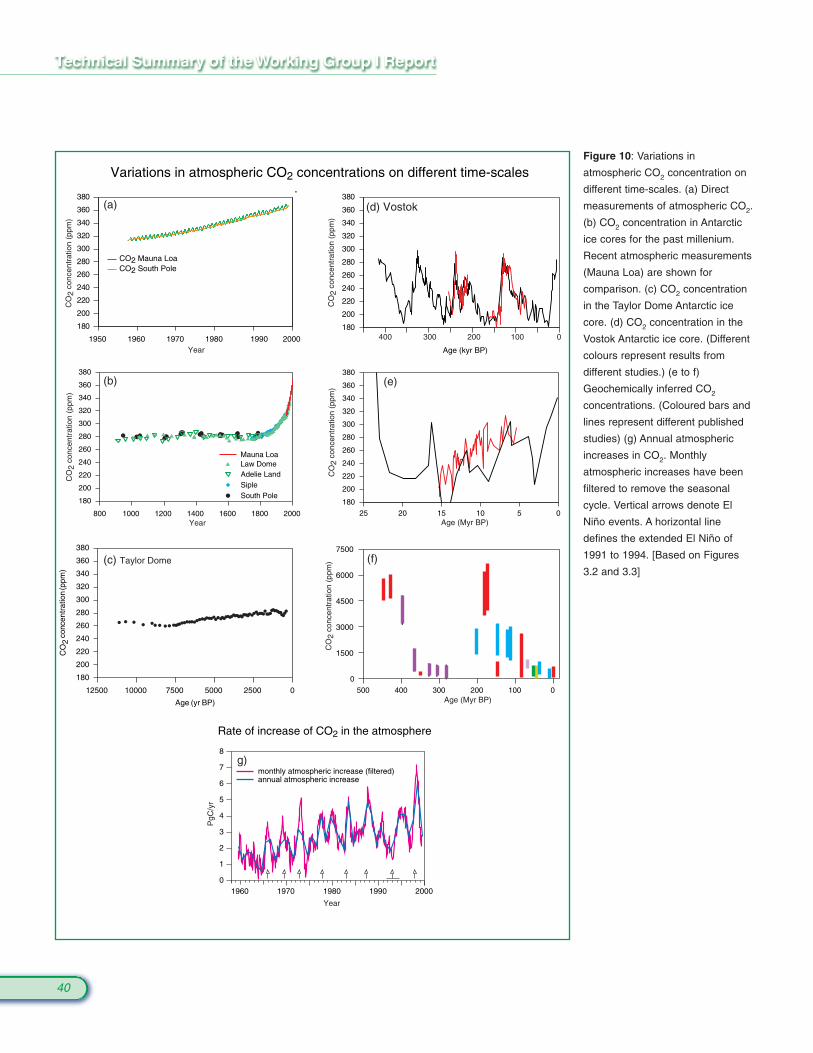
40

180

200

220

240

260

280

300

320

340

360

380

12500 10000 7500 5000 2500 0

Age (yr BP)

(c) Taylor Dome

CO

2co

ncen

trat

ion

(ppm

)

180

200

220

240

260

280

300

320

340

360

380

Age (kyr BP)

0100200300400

(d) Vostok

CO

2 co

ncen

trat

ion

(ppm

)180

200

220

240

260

280

300

320

340

360

380

1950 1960 1970 1980 1990 2000

CO2 Mauna LoaCO2 South Pole

Year

CO

2 co

ncen

trat

ion

(ppm

)

(a)

Year

CO

2 co

ncen

trat

ion

(ppm

)

180

200

220

240

260

280

300

320

340

360

380

800 1000 1200 1400 1600 1800 2000

Law Dome Adelie LandSipleSouth Pole

Mauna Loa

(b)

1500

3000

4500

6000

7500

Age (Myr BP)

CO

2 co

ncen

trat

ion

(ppm

) (f)

g)

Age (Myr BP)

CO

2 co

ncen

trat

ion

(ppm

)

180

200

220

240

260

280

300

320

340

360

380

25 20 15 10 5 0

(e)

0

500 400 300 200 100 0

0

1

2

3

4

5

6

7

8

1960 1970 1980 1990 2000

fossil fuel emissionsannual atmospheric increasemonthly atmospheric increase (filtered)

PgC

/yr

Year

Rate of increase of CO2 in the atmosphere

Variations in atmospheric CO2 concentrations on different time-scalesFigure 10: Variations in

atmospheric CO2 concentration on

different time-scales. (a) Direct

measurements of atmospheric CO2.

(b) CO2 concentration in Antarctic

ice cores for the past millenium.

Recent atmospheric measurements

(Mauna Loa) are shown for

comparison. (c) CO2 concentration

in the Taylor Dome Antarctic ice

core. (d) CO2 concentration in the

Vostok Antarctic ice core. (Different

colours represent results from

different studies.) (e to f)

Geochemically inferred CO2

concentrations. (Coloured bars and

lines represent different published

studies) (g) Annual atmospheric

increases in CO2. Monthly

atmospheric increases have been

filtered to remove the seasonal

cycle. Vertical arrows denote El

Niño events. A horizontal line

defines the extended El Niño of

1991 to 1994. [Based on Figures

3.2 and 3.3]

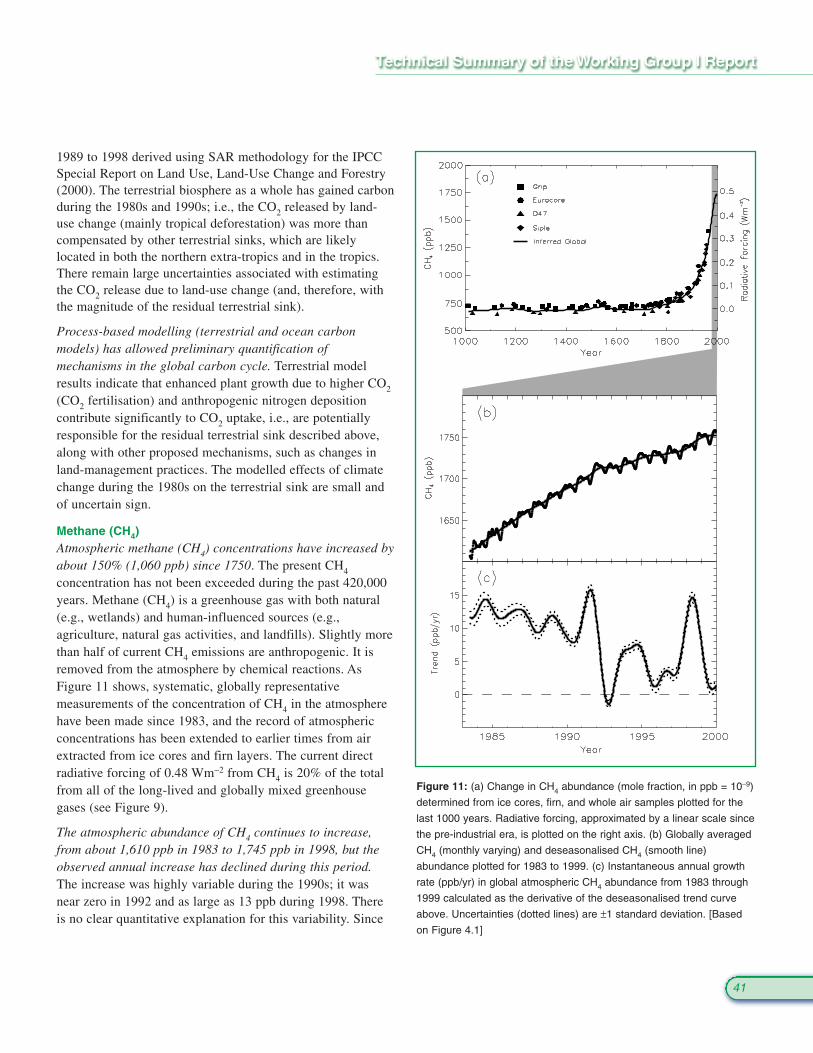
41

1989 to 1998 derived using SAR methodology for the IPCCSpecial Report on Land Use, Land-Use Change and Forestry(2000). The terrestrial biosphere as a whole has gained carbonduring the 1980s and 1990s; i.e., the CO2 released by land-use change (mainly tropical deforestation) was more thancompensated by other terrestrial sinks, which are likelylocated in both the northern extra-tropics and in the tropics.There remain large uncertainties associated with estimatingthe CO2 release due to land-use change (and, therefore, withthe magnitude of the residual terrestrial sink).

Process-based modelling (terrestrial and ocean carbonmodels) has allowed preliminary quantification ofmechanisms in the global carbon cycle. Terrestrial modelresults indicate that enhanced plant growth due to higher CO2

(CO2 fertilisation) and anthropogenic nitrogen depositioncontribute significantly to CO2 uptake, i.e., are potentiallyresponsible for the residual terrestrial sink described above,along with other proposed mechanisms, such as changes inland-management practices. The modelled effects of climatechange during the 1980s on the terrestrial sink are small andof uncertain sign.

Methane (CH4)Atmospheric methane (CH4) concentrations have increased byabout 150% (1,060 ppb) since 1750. The present CH4

concentration has not been exceeded during the past 420,000years. Methane (CH4) is a greenhouse gas with both natural(e.g., wetlands) and human-influenced sources (e.g.,agriculture, natural gas activities, and landfills). Slightly morethan half of current CH4 emissions are anthropogenic. It isremoved from the atmosphere by chemical reactions. AsFigure 11 shows, systematic, globally representativemeasurements of the concentration of CH4 in the atmospherehave been made since 1983, and the record of atmosphericconcentrations has been extended to earlier times from airextracted from ice cores and firn layers. The current directradiative forcing of 0.48 Wm−2 from CH4 is 20% of the totalfrom all of the long-lived and globally mixed greenhousegases (see Figure 9).

The atmospheric abundance of CH4 continues to increase,from about 1,610 ppb in 1983 to 1,745 ppb in 1998, but theobserved annual increase has declined during this period.The increase was highly variable during the 1990s; it wasnear zero in 1992 and as large as 13 ppb during 1998. Thereis no clear quantitative explanation for this variability. Since

Figure 11: (a) Change in CH4 abundance (mole fraction, in ppb = 10−9)

determined from ice cores, firn, and whole air samples plotted for the

last 1000 years. Radiative forcing, approximated by a linear scale since

the pre-industrial era, is plotted on the right axis. (b) Globally averaged

CH4 (monthly varying) and deseasonalised CH4 (smooth line)

abundance plotted for 1983 to 1999. (c) Instantaneous annual growth

rate (ppb/yr) in global atmospheric CH4 abundance from 1983 through

1999 calculated as the derivative of the deseasonalised trend curve

above. Uncertainties (dotted lines) are ±1 standard deviation. [Based

on Figure 4.1]

brought the source/sink estimates closer in balance, comparedwith the SAR. However, the predictive understandingassociated with this significant, long-lived greenhouse gas hasnot improved significantly since the last assessment. Theradiative forcing is estimated at 0.15 Wm−2, which is 6% ofthe total from all of the long-lived and globally mixedgreenhouse gases (see Figure 9).

Halocarbons and related compoundsThe atmospheric concentrations of many of those gases thatare both ozone-depleting and greenhouse gases are eitherdecreasing (CFC-11, CFC-113, CH3CCl3 and CCl4) orincreasing more slowly (CFC-12) in response to reducedemissions under the regulations of the Montreal Protocol andits Amendments. Many of these halocarbons are alsoradiatively effective, long-lived greenhouse gases.Halocarbons are carbon compounds that contain fluorine,chlorine, bromine or iodine. For most of these compounds,human activities are the sole source. Halocarbons thatcontain chlorine (e.g., chlorofluorocarbons - CFCs) andbromine (e.g., halons) cause depletion of the stratosphericozone layer and are controlled under the Montreal Protocol.The combined tropospheric abundance of ozone-depletinggases peaked in 1994 and is slowly declining. Theatmospheric abundances of some of the major greenhousehalocarbons have peaked, as shown for CFC-11 in Figure 12.The concentrations of CFCs and chlorocarbons in thetroposphere are consistent with reported emissions.Halocarbons contribute a radiative forcing of 0.34 Wm−2,which is 14% of the radiative forcing from all of the globallymixed greenhouse gases (Figure 9).

The observed atmospheric concentrations of the substitutes forthe CFCs are increasing, and some of these compounds aregreenhouse gases. The abundances of the hydrochlorofluoro-carbons (HCFCs) and hydrofluorocarbons (HFCs) areincreasing as a result of continuation of earlier uses and oftheir use as substitutes for the CFCs. For example, the concen-tration of HFC-23 has increased by more than a factor of threebetween 1978 and 1995. Because current concentrations arerelatively low, the present contribution of HFCs to radiativeforcing is relatively small. The present contribution of HCFCsto radiative forcing is also relatively small, and futureemissions of these gases are limited by the Montreal Protocol.

The perfluorocarbons (PFCs, e.g., CF4 and C2F6) and sulphurhexafluoride (SF6) have anthropogenic sources, have extremely

42

the SAR, quantification of certain anthropogenic sources ofCH4, such as that from rice production, has improved.

The rate of increase in atmospheric CH4 is due to a smallimbalance between poorly characterised sources and sinks,which makes the prediction of future concentrationsproblematic. Although the major contributors to the globalCH4 budget likely have been identified, most of them are quiteuncertain quantitatively because of the difficulty in assessingemission rates of highly variable biospheric sources. Thelimitations of poorly quantified and characterised CH4 sourcestrengths inhibit the prediction of future CH4 atmosphericconcentrations (and hence its contribution to radiative forcing)for any given anthropogenic emission scenario, particularlysince both natural emissions and the removal of CH4 can beinfluenced substantially by climate change.

Nitrous oxide (N2O)The atmospheric concentration of nitrous oxide (N2O) hassteadily increased during the Industrial Era and is now 16%(46 ppb) larger than in 1750. The present N2O concentrationhas not been exceeded during at least the past thousand years.Nitrous oxide is another greenhouse gas with both natural andanthropogenic sources, and it is removed from the atmosphereby chemical reactions. Atmospheric concentrations of N2Ocontinue to increase at a rate of 0.25%/yr (1980 to 1998).Significant interannual variations in the upward trend of N2Oconcentrations are observed, e.g., a 50% reduction in annualgrowth rate from 1991 to 1993. Suggested causes are several-fold: a decrease in use of nitrogen-based fertiliser, lowerbiogenic emissions, and larger stratospheric losses due tovolcanic-induced circulation changes. Since 1993, the growthof N2O concentrations has returned to rates closer to thoseobserved during the 1980s. While this observed multi-yearvariance has provided some potential insight into whatprocesses control the behaviour of atmospheric N2O, themulti-year trends of this greenhouse gas remain largelyunexplained.

The global budget of nitrous oxide is in better balance than inthe SAR, but uncertainties in the emissions from individualsources are still quite large. Natural sources of N2O areestimated to be approximately 10 TgN/yr (1990), with soilsbeing about 65% of the sources and oceans about 30%. New, higher estimates of the emissions from anthropogenicsources (agriculture, biomass burning, industrial activities,and livestock management) of approximately 7 TgN/yr have

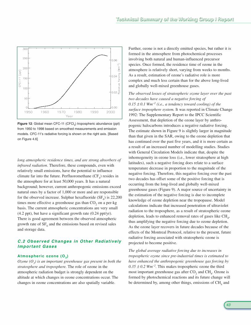
Further, ozone is not a directly emitted species, but rather it isformed in the atmosphere from photochemical processesinvolving both natural and human-influenced precursorspecies. Once formed, the residence time of ozone in theatmosphere is relatively short, varying from weeks to months.As a result, estimation of ozone’s radiative role is morecomplex and much less certain than for the above long-livedand globally well-mixed greenhouse gases.

The observed losses of stratospheric ozone layer over the pasttwo decades have caused a negative forcing of 0.15 ± 0.1 Wm−2 (i.e., a tendency toward cooling) of thesurface troposphere system. It was reported in Climate Change1992: The Supplementary Report to the IPCC ScientificAssessment, that depletion of the ozone layer by anthro-pogenic halocarbons introduces a negative radiative forcing.The estimate shown in Figure 9 is slightly larger in magnitudethan that given in the SAR, owing to the ozone depletion thathas continued over the past five years, and it is more certain asa result of an increased number of modelling studies. Studieswith General Circulation Models indicate that, despite theinhomogeneity in ozone loss (i.e., lower stratosphere at highlatitudes), such a negative forcing does relate to a surfacetemperature decrease in proportion to the magnitude of thenegative forcing. Therefore, this negative forcing over the pasttwo decades has offset some of the positive forcing that isoccurring from the long-lived and globally well-mixedgreenhouse gases (Figure 9). A major source of uncertainty inthe estimation of the negative forcing is due to incompleteknowledge of ozone depletion near the tropopause. Modelcalculations indicate that increased penetration of ultravioletradiation to the troposphere, as a result of stratospheric ozonedepletion, leads to enhanced removal rates of gases like CH4,thus amplifying the negative forcing due to ozone depletion.As the ozone layer recovers in future decades because of theeffects of the Montreal Protocol, relative to the present, futureradiative forcing associated with stratospheric ozone isprojected to become positive.

The global average radiative forcing due to increases intropospheric ozone since pre-industrial times is estimated tohave enhanced the anthropogenic greenhouse gas forcing by0.35 ± 0.2 Wm−2. This makes tropospheric ozone the thirdmost important greenhouse gas after CO2 and CH4. Ozone isformed by photochemical reactions and its future change willbe determined by, among other things, emissions of CH4 and

43

long atmospheric residence times, and are strong absorbers ofinfrared radiation. Therefore, these compounds, even withrelatively small emissions, have the potential to influenceclimate far into the future. Perfluoromethane (CF4) resides inthe atmosphere for at least 50,000 years. It has a naturalbackground; however, current anthropogenic emissions exceednatural ones by a factor of 1,000 or more and are responsiblefor the observed increase. Sulphur hexafluoride (SF6) is 22,200times more effective a greenhouse gas than CO2 on a per-kgbasis. The current atmospheric concentrations are very small(4.2 ppt), but have a significant growth rate (0.24 ppt/yr).There is good agreement between the observed atmosphericgrowth rate of SF6 and the emissions based on revised salesand storage data.

C.2 Observed Changes in Other Radiat ivelyImpor tant Gases

Atmospheric ozone (O3)Ozone (O3) is an important greenhouse gas present in both thestratosphere and troposphere. The role of ozone in theatmospheric radiation budget is strongly dependent on thealtitude at which changes in ozone concentrations occur. Thechanges in ozone concentrations are also spatially variable.

Figure 12: Global mean CFC-11 (CFCl3) tropospheric abundance (ppt)

from 1950 to 1998 based on smoothed measurements and emission

models. CFC-11's radiative forcing is shown on the right axis. [Based

on Figure 4.6]

of the reaction products of NOx fertilises the biosphere,thereby decreasing atmospheric CO2. While difficult toquantify, increases in NOx that are projected to the year 2100would cause significant changes in greenhouse gases.

C.3 Observed and Model led Changes inAerosols

Aerosols (very small airborne particles and droplets) areknown to influence significantly the radiative budget of theEarth/atmosphere. Aerosol radiative effects occur in twodistinct ways: (i) the direct effect, whereby aerosolsthemselves scatter and absorb solar and thermal infraredradiation, and (ii) the indirect effect, whereby aerosolsmodify the microphysical and hence the radiative propertiesand amount of clouds. Aerosols are produced by a variety ofprocesses, both natural (including dust storms and volcanicactivity) and anthropogenic (including fossil fuel andbiomass burning). The atmospheric concentrations of tropospheric aerosols are thought to have increased overrecent years due to increased anthropogenic emissions ofparticles and their precursor gases, hence giving rise toradiative forcing. Most aerosols are found in the lowertroposphere (below a few kilometres), but the radiative effectof many aerosols is sensitive to the vertical distribution.Aerosols undergo chemical and physical changes while in theatmosphere, notably within clouds, and are removed largelyand relatively rapidly by precipitation (typically within aweek). Because of this short residence time and the inhomogeneity of sources, aerosols are distributed inhomogeneously in the troposphere, with maxima near thesources. The radiative forcing due to aerosols depends notonly on these spatial distributions, but also on the size,shape, and chemical composition of the particles and variousaspects (e.g., cloud formation) of the hydrological cycle aswell. As a result of all of these factors, obtaining accurateestimates of this forcing has been very challenging, fromboth the observational and theoretical standpoints.

Nevertheless, substantial progress has been achieved in betterdefining the direct effect of a wider set of different aerosols. TheSAR considered the direct effects of only three anthropogenicaerosol species: sulphate aerosols, biomass-burning aerosols,and fossil fuel black carbon (or soot). Observations have nowshown the importance of organic materials in both fossil fuelcarbon aerosols and biomass-burning carbon aerosols. Since

44

pollutants (as noted below). Ozone concentrations respondrelatively quickly to changes in the emissions of pollutants. Onthe basis of limited observations and several modelling studies,tropospheric ozone is estimated to have increased by about35% since the Pre-industrial Era, with some regions experi-encing larger and some with smaller increases. There havebeen few observed increases in ozone concentrations in theglobal troposphere since the mid-1980s at most of the fewremote locations where it is regularly measured. The lack ofobserved increase over North America and Europe is related tothe lack of a sustained increase in ozone-precursor emissionsfrom those continents. However, some Asian stations indicatea possible rise in tropospheric ozone, which could be related tothe increase in East Asian emissions. As a result of moremodelling studies than before, there is now an increasedconfidence in the estimates of tropospheric ozone forcing. Theconfidence, however, is still much less than that for the well-mixedgreenhouse gases, but more so than that for aerosol forcing.Uncertainties arise because of limited information on pre-industrialozone distributions and limited information to evaluatemodelled global trends in the modern era (i.e., post-1960).

Gases with only indirect radiat ive inf luencesSeveral chemically reactive gases, including reactive nitrogenspecies (NOx), carbon monoxide (CO), and the volatile organiccompounds (VOCs), control, in part, the oxidising capacity ofthe troposphere, as well as the abundance of ozone. Thesepollutants act as indirect greenhouse gases through theirinfluence not only on ozone, but also on the lifetimes of CH4

and other greenhouse gases. The emissions of NOx and CO aredominated by human activities.

Carbon monoxide is identified as an important indirectgreenhouse gas. Model calculations indicate that emission of 100 Mt of CO is equivalent in terms of greenhouse gas perturbations to the emission of about 5 Mt of CH4. Theabundance of CO in the Northern Hemisphere is about twice thatin the Southern Hemisphere and has increased in the second halfof the 20th century along with industrialisation and population.

The reactive nitrogen species NO and NO2, (whose sum isdenoted NOx), are key compounds in the chemistry of thetroposphere, but their overall radiative impact remainsdifficult to quantify. The importance of NOx in the radiationbudget is because increases in NOx concentrations perturbseveral greenhouse gases; for example, decreases in methaneand the HFCs and increases in tropospheric ozone. Deposition

magnitude of any such indirect effect is not known, although itis likely to be positive. It is not possible to estimate the numberof anthropogenic ice nuclei at the present time. Except at coldtemperatures (below −45°C) where homogeneous nucleation isexpected to dominate, the mechanisms of ice formation inthese clouds are not yet known.

C.4 Observed Changes in OtherAnthropogenic Forcing Agents

Land-use (albedo) changeChanges in land use, deforestation being the major factor,appear to have produced a negative radiative forcing of −0.2 ± 0.2 Wm−2 (Figure 8). The largest effect is estimated to beat the high latitudes. This is because deforestation has causedsnow-covered forests with relatively low albedo to be replacedwith open, snow-covered areas with higher albedo. The estimategiven above is based on simulations in which pre-industrialvegetation is replaced by current land-use patterns. However, thelevel of understanding is very low for this forcing, and therehave been far fewer investigations of this forcing compared toinvestigations of other factors considered in this report.

C.5 Observed and Model led Changes inSolar and Volcanic Act iv i ty

Radiative forcing of the climate system due to solar irradiancechange is estimated to be 0.3 ± 0.2 Wm−2 for the period 1750to the present (Figure 8), and most of the change is estimatedto have occurred during the first half of the 20th century. Thefundamental source of all energy in the Earth’s climate systemis radiation from the Sun. Therefore, variation in solar outputis a radiative forcing agent. The absolute value of thespectrally integrated total solar irradiance (TSI) incident on theEarth is not known to better than about 4 Wm−2, but satelliteobservations since the late 1970s show relative variations overthe past two solar 11-year activity cycles of about 0.1%, whichis equivalent to a variation in radiative forcing of about 0.2Wm−2. Prior to these satellite observations, reliable directmeasurements of solar irradiance are not available. Variationsover longer periods may have been larger, but the techniquesused to reconstruct historical values of TSI from proxyobservations (e.g., sunspots) have not been adequately verified.Solar variation varies more substantially in the ultravioletregion, and studies with climate models suggest that inclusionof spectrally resolved solar irradiance variations and solar-

45

the SAR, the inclusion of estimates for the abundance offossil fuel organic carbon aerosols has led to an increase inthe predicted total optical depth (and consequent negativeforcing) associated with industrial aerosols. Advances inobservations and in aerosol and radiative models have allowedquantitative estimates of these separate components, as wellas an estimate for the range of radiative forcing associatedwith mineral dust, as shown in Figure 9. Direct radiativeforcing is estimated to be −0.4 Wm−2 for sulphate,−0.2 Wm−2 for biomass-burning aerosols, −0.1 Wm−2 forfossil fuel organic carbon, and +0.2 Wm−2 for fossil fuel blackcarbon aerosols. Uncertainties remain relatively large,however. These arise from difficulties in determining theconcentration and radiative characteristics of atmosphericaerosols and the fraction of the aerosols that are of anthropogenicorigin, particularly the knowledge of the sources ofcarbonaceous aerosols. This leads to considerable differences(i.e., factor of two to three range) in the burden andsubstantial differences in the vertical distribution (factor often). Anthropogenic dust aerosol is also poorly quantified.Satellite observations, combined with model calculations, areenabling the identification of the spatial signature of the totalaerosol radiative effect in clear skies; however, the quanti-tative amount is still uncertain.

Estimates of the indirect radiative forcing by anthropogenicaerosols remain problematic, although observational evidencepoints to a negative aerosol-induced indirect forcing in warmclouds. Two different approaches exist for estimating theindirect effect of aerosols: empirical methods and mechanisticmethods. The former have been applied to estimate the effectsof industrial aerosols, while the latter have been applied toestimate the effects of sulphate, fossil fuel carbonaceousaerosols, and biomass aerosols. In addition, models for theindirect effect have been used to estimate the effects of theinitial change in droplet size and concentrations (a firstindirect effect), as well as the effects of the subsequent changein precipitation efficiency (a second indirect effect). Thestudies represented in Figure 9 provide an expert judgementfor the range of the first of these; the range is now slightlywider than in the SAR; the radiative perturbation associatedwith the second indirect effect is of the same sign and could beof similar magnitude compared to the first effect.

The indirect radiative effect of aerosols is now understood toalso encompass effects on ice and mixed-phase clouds, but the

D. The Simulat ion of the Cl imateSystem and i ts Changes

The preceding two Sections reported on the climate from thedistant past to the present day through the observations ofclimate variables and the forcing agents that cause climate tochange. This Section bridges to the climate of the future bydescribing the only tool that provides quantitative estimates offuture climate changes, namely, numerical models. The basicunderstanding of the energy balance of the Earth system meansthat quite simple models can provide a broad quantitativeestimate of some globally averaged variables, but more accurateestimates of feedbacks and of regional detail can only come frommore elaborate climate models. The complexity of the processesin the climate system prevents the use of extrapolation of pasttrends or statistical and other purely empirical techniques forprojections. Climate models can be used to simulate the climateresponses to different input scenarios of future forcing agents(Section F). Similarly, projection of the fate of emitted CO2 (i.e.,the relative sequestration into the various reservoirs) and othergreenhouse gases requires an understanding of the biogeo-chemical processes involved and incorporating these into anumerical carbon cycle model.

A climate model is a simplified mathematical representation ofthe Earth’s climate system (see Box 3). The degree to which themodel can simulate the responses of the climate system hinges toa very large degree on the level of understanding of the physical,geophysical, chemical and biological processes that govern theclimate system. Since the SAR, researchers have madesubstantial improvements in the simulation of the Earth’s climatesystem with models. First, the current understanding of some ofthe most important processes that govern the climate system andhow well they are represented in present climate models aresummarised here. Then, this Section presents an assessment ofthe overall ability of present models to make useful projectionsof future climate.

D.1 Climate Processes and Feedbacks

Processes in the climate system determine the naturalvariability of the climate system and its response to perturbations,such as the increase in the atmospheric concentrations ofgreenhouse gases. Many basic climate processes of importanceare well-known and modelled exceedingly well. Feedbackprocesses amplify (a positive feedback) or reduce (a negative

46

induced stratospheric ozone changes may improve the realismof model simulations of the impact of solar variability onclimate. Other mechanisms for the amplification of solareffects on climate have been proposed, but do not have arigorous theoretical or observational basis.

Stratospheric aerosols from explosive volcanic eruptions leadto negative forcing that lasts a few years. Several explosiveeruptions occurred in the periods 1880 to 1920 and 1960 to1991, and no explosive eruptions since 1991. Enhancedstratospheric aerosol content due to volcanic eruptions,together with the small solar irradiance variations, result in anet negative natural radiative forcing over the past two, andpossibly even the past four, decades.

C.6 Global Warming Potent ia ls

Radiative forcings and Global Warming Potentials (GWPs) arepresented in Table 3 for an expanded set of gases. GWPs are ameasure of the relative radiative effect of a given substancecompared to CO2, integrated over a chosen time horizon. Newcategories of gases in Table 3 include fluorinated organicmolecules, many of which are ethers that are proposed ashalocarbon substitutes. Some of the GWPs have largeruncertainties than that of others, particularly for those gaseswhere detailed laboratory data on lifetimes are not yetavailable. The direct GWPs have been calculated relative toCO2 using an improved calculation of the CO2 radiativeforcing, the SAR response function for a CO2 pulse, and newvalues for the radiative forcing and lifetimes for a number ofhalocarbons. Indirect GWPs, resulting from indirect radiativeforcing effects, are also estimated for some new gases,including carbon monoxide. The direct GWPs for those specieswhose lifetimes are well characterised are estimated to beaccurate within ±35%, but the indirect GWPs are less certain.

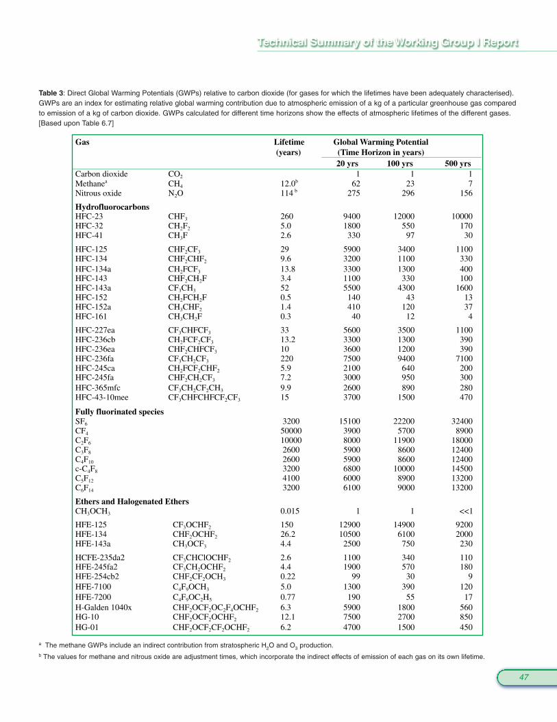
Table 3: Direct Global Warming Potentials (GWPs) relative to carbon dioxide (for gases for which the lifetimes have been adequately characterised).GWPs are an index for estimating relative global warming contribution due to atmospheric emission of a kg of a particular greenhouse gas comparedto emission of a kg of carbon dioxide. GWPs calculated for different time horizons show the effects of atmospheric lifetimes of the different gases.[Based upon Table 6.7]

47

Gas Lifetime (years)

Global Warming Potential (Time Horizon in years)

20 yrs 100 yrs 500 yrsCarbon dioxide CO2 1 1 1Methanea CH4 12.0b 62 23 7Nitrous oxide N2O 114 b 275 296 156

HydrofluorocarbonsHFC-23 CHF3 260 9400 12000 10000HFC-32 CH2F2 5.0 1800 550 170HFC-41 CH3F 2.6 330 97 30

HFC-125 CHF2CF3 29 5900 3400 1100HFC-134 CHF2CHF2 9.6 3200 1100 330HFC-134a CH2FCF3 13.8 3300 1300 400HFC-143 CHF2CH2F 3.4 1100 330 100HFC-143a CF3CH3 52 5500 4300 1600HFC-152 CH2FCH2F 0.5 140 43 13HFC-152a CH3CHF2 1.4 410 120 37HFC-161 CH3CH2F 0.3 40 12 4

HFC-227ea CF3CHFCF3 33 5600 3500 1100HFC-236cb CH2FCF2CF3 13.2 3300 1300 390HFC-236ea CHF2CHFCF3 10 3600 1200 390HFC-236fa CF3CH2CF3 220 7500 9400 7100HFC-245ca CH2FCF2CHF2 5.9 2100 640 200HFC-245fa CHF2CH2CF3 7.2 3000 950 300HFC-365mfc CF3CH2CF2CH3 9.9 2600 890 280HFC-43-10mee CF3CHFCHFCF2CF3 15 3700 1500 470

Fully fluorinated speciesSF6 3200 15100 22200 32400CF4 50000 3900 5700 8900C2F6 10000 8000 11900 18000C3F8 2600 5900 8600 12400C4F10 2600 5900 8600 12400c-C4F8 3200 6800 10000 14500C5F12 4100 6000 8900 13200C6F14 3200 6100 9000 13200

Ethers and Halogenated EthersCH3OCH3 0.015 1 1 <<1

HFE-125 CF3OCHF2 150 12900 14900 9200HFE-134 CHF2OCHF2 26.2 10500 6100 2000HFE-143a CH3OCF3 4.4 2500 750 230

HCFE-235da2 CF3CHClOCHF2 2.6 1100 340 110HFE-245fa2 CF3CH2OCHF2 4.4 1900 570 180HFE-254cb2 CHF2CF2OCH3 0.22 99 30 9HFE-7100 C4F9OCH3 5.0 1300 390 120HFE-7200 C4F9OC2H5 0.77 190 55 17H-Galden 1040x CHF2OCF2OC2F4OCHF2 6.3 5900 1800 560HG-10 CHF2OCF2OCHF2 12.1 7500 2700 850HG-01 CHF2OCF2CF2OCHF2 6.2 4700 1500 450

a The methane GWPs include an indirect contribution from stratospheric H2O and O3 production. b The values for methane and nitrous oxide are adjustment times, which incorporate the indirect effects of emission of each gas on its own lifetime.

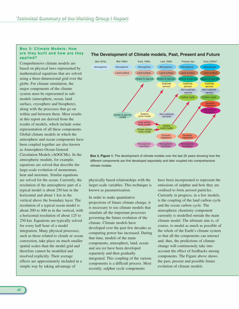
48

Box 3: Cl imate Models: Howare they bui l t and how are theyappl ied?

Comprehensive climate models arebased on physical laws represented bymathematical equations that are solvedusing a three-dimensional grid over theglobe. For climate simulation, themajor components of the climatesystem must be represented in sub-models (atmosphere, ocean, landsurface, cryosphere and biosphere),along with the processes that go onwithin and between them. Most resultsin this report are derived from theresults of models, which include somerepresentation of all these components.Global climate models in which theatmosphere and ocean components havebeen coupled together are also knownas Atmosphere-Ocean GeneralCirculation Models (AOGCMs). In theatmospheric module, for example,equations are solved that describe thelarge-scale evolution of momentum,heat and moisture. Similar equationsare solved for the ocean. Currently, theresolution of the atmospheric part of atypical model is about 250 km in thehorizontal and about 1 km in thevertical above the boundary layer. Theresolution of a typical ocean model isabout 200 to 400 m in the vertical, witha horizontal resolution of about 125 to250 km. Equations are typically solvedfor every half hour of a modelintegration. Many physical processes,such as those related to clouds or oceanconvection, take place on much smallerspatial scales than the model grid andtherefore cannot be modelled andresolved explicitly. Their averageeffects are approximately included in asimple way by taking advantage of

physically based relationships with thelarger-scale variables. This technique isknown as parametrization.

In order to make quantitativeprojections of future climate change, itis necessary to use climate models thatsimulate all the important processesgoverning the future evolution of theclimate. Climate models havedeveloped over the past few decades ascomputing power has increased. Duringthat time, models of the maincomponents, atmosphere, land, oceanand sea ice have been developedseparately and then graduallyintegrated. This coupling of the variouscomponents is a difficult process. Mostrecently, sulphur cycle components

have been incorporated to represent theemissions of sulphur and how they areoxidised to form aerosol particles.Currently in progress, in a few models,is the coupling of the land carbon cycleand the ocean carbon cycle. Theatmospheric chemistry componentcurrently is modelled outside the mainclimate model. The ultimate aim is, ofcourse, to model as much as possible ofthe whole of the Earth’s climate systemso that all the components can interactand, thus, the predictions of climatechange will continuously take intoaccount the effect of feedbacks amongcomponents. The Figure above showsthe past, present and possible futureevolution of climate models.

Atmosphere Atmosphere Atmosphere Atmosphere Atmosphere Atmosphere

Land surfaceLand surfaceLand surfaceLand surfaceLand surface

Ocean & sea-ice Ocean & sea-ice Ocean & sea-ice Ocean & sea-ice

Sulphateaerosol

Sulphateaerosol

Sulphateaerosol

Non-sulphateaerosol

Non-sulphateaerosol

Carbon cycle Carbon cycle

Atmosphericchemistry

Ocean & sea-icemodel

Sulphurcycle model

Non-sulphateaerosols

Carboncycle model

Land carboncycle model

Ocean carboncycle model



Dynamicvegetation

Dynamicvegetation

Dynamicvegetation


Mid-1970s Mid-1980s Early 1990s Late 1990s Present day Early 2000s?

The Development of Climate models, Past, Present and Future

Box 3, Figure 1: The development of climate models over the last 25 years showing how the

different components are first developed separately and later coupled into comprehensive

climate models.

49

Some models offset errors and surface flux imbalancesthrough “flux adjustments”, which are empiricallydetermined systematic adjustments at the atmosphere-ocean interface held fixed in time in order to bring thesimulated climate closer to the observed state. A strategyhas been designed for carrying out climate experimentsthat removes much of the effects of some model errors onresults. What is often done is that first a “control” climatesimulation is run with the model. Then, the climatechange experiment simulation is run, for example, withincreased CO2 in the model atmosphere. Finally, thedifference is taken to provide an estimate of the change inclimate due to the perturbation. The differencingtechnique removes most of the effects of any artificialadjustments in the model, as well as systematic errors thatare common to both runs. However, a comparison ofdifferent model results makes it apparent that the natureof some errors still influences the outcome.

Many aspects of the Earth’s climate system are chaotic –its evolution is sensitive to small perturbations in initialconditions. This sensitivity limits predictability of thedetailed evolution of weather to about two weeks.However, predictability of climate is not so limitedbecause of the systematic influences on the atmosphere ofthe more slowly varying components of the climatesystem. Nevertheless, to be able to make reliable forecastsin the presence of both initial condition and modeluncertainty, it is desirable to repeat the prediction manytimes from different perturbed initial states and usingdifferent global models. These ensembles are the basis ofprobability forecasts of the climate state.

Comprehensive AOGCMs are very complex and takelarge computer resources to run. To explore differentscenarios of emissions of greenhouse gases and theeffects of assumptions or approximations in parameters inthe model more thoroughly, simpler models are alsowidely used. The simplifications may include coarserresolution and simplified dynamics and physicalprocesses. Together, simple, intermediate, and compre-hensive models form a “hierarchy of climate models”, allof which are necessary to explore choices made inparametrizations and assess the robustness of climatechanges.

feedback) changes in response to an initial perturbation andhence are very important for accurate simulation of theevolution of climate.

Water vapourA major feedback accounting for the large warming predicted byclimate models in response to an increase in CO2 is the increasein atmospheric water vapour. An increase in the temperature ofthe atmosphere increases its water-holding capacity; however,since most of the atmosphere is undersaturated, this does notautomatically mean that water vapour, itself, must increase.Within the boundary layer (roughly the lowest 1 to 2 km of theatmosphere), water vapour increases with increasing temperature.In the free troposphere above the boundary layer, where thewater vapour greenhouse effect is most important, the situation isharder to quantify. Water vapour feedback, as derived fromcurrent models, approximately doubles the warming from what itwould be for fixed water vapour. Since the SAR, majorimprovements have occurred in the treatment of water vapour inmodels, although detrainment of moisture from clouds remainsquite uncertain and discrepancies exist between model watervapour distributions and those observed. Models are capable ofsimulating the moist and very dry regions observed in the tropicsand sub-tropics and how they evolve with the seasons and fromyear to year. While reassuring, this does not provide a check ofthe feedbacks, although the balance of evidence favours apositive clear-sky water vapour feedback of the magnitudecomparable to that found in simulations.

CloudsAs has been the case since the first IPCC Assessment Report in1990, probably the greatest uncertainty in future projections ofclimate arises from clouds and their interactions with radiation.Clouds can both absorb and reflect solar radiation (therebycooling the surface) and absorb and emit long wave radiation(thereby warming the surface). The competition between theseeffects depends on cloud height, thickness and radiativeproperties. The radiative properties and evolution of cloudsdepend on the distribution of atmospheric water vapour, waterdrops, ice particles, atmospheric aerosols and cloud thickness.The physical basis of cloud parametrizations is greatly improvedin models through inclusion of bulk representation of cloudmicrophysical properties in a cloud water budget equation,although considerable uncertainty remains. Clouds represent asignificant source of potential error in climate simulations. Thepossibility that models underestimate systematically solar

50

absorption in clouds remains a controversial matter. The sign ofthe net cloud feedback is still a matter of uncertainty, and thevarious models exhibit a large spread. Further uncertainties arisefrom precipitation processes and the difficulty in correctlysimulating the diurnal cycle and precipitation amounts andfrequencies.

StratosphereThere has been a growing appreciation of the importance ofthe stratosphere in the climate system because of changes inits structure and recognition of the vital role of both radiativeand dynamical processes. The vertical profile of temperaturechange in the atmosphere, including the stratosphere, is animportant indicator in detection and attribution studies. Mostof the observed decreases in lower-stratospheric temperatureshave been due to ozone decreases, of which the Antarctic“ozone hole” is a part, rather than increased CO2 concen-trations. Waves generated in the troposphere can propagateinto the stratosphere where they are absorbed. As a result,stratospheric changes alter where and how these waves areabsorbed, and the effects can extend downward into thetroposphere. Changes in solar irradiance, mainly in theultraviolet (UV), lead to photochemically-induced ozonechanges and, hence, alter the stratospheric heating rates, whichcan alter the tropospheric circulation. Limitations in resolutionand relatively poor representation of some stratosphericprocesses adds uncertainty to model results.

Ocean Major improvements have taken place in modelling oceanprocesses, in particular heat transport. These improvements, inconjunction with an increase in resolution, have beenimportant in reducing the need for flux adjustment in modelsand in producing realistic simulations of natural large-scalecirculation patterns and improvements in simulating El Niño(see Box 4). Ocean currents carry heat from the tropics tohigher latitudes. The ocean exchanges heat, water (throughevaporation and precipitation) and CO2 with the atmosphere.Because of its huge mass and high heat capacity, the oceanslows climate change and influences the time-scales ofvariability in the ocean-atmosphere system. Considerableprogress has been made in the understanding of oceanprocesses relevant for climate change. Increases in resolution,as well as improved representation (parametrization) ofimportant sub-grid scale processes (e.g., mesoscale eddies),have increased the realism of simulations. Major uncertainties

still exist with the representation of small-scale processes, suchas overflows (flow through narrow channels, e.g., betweenGreenland and Iceland), western boundary currents (i.e., large-scale narrow currents along coastlines), convection and mixing.Boundary currents in climate simulations are weaker and widerthan in nature, although the consequences of this for climateare not clear.

Cryosphere The representation of sea-ice processes continues to improve,with several climate models now incorporating physically basedtreatments of ice dynamics. The representation of land-iceprocesses in global climate models remains rudimentary. Thecryosphere consists of those regions of Earth that are seasonallyor perennially covered by snow and ice. Sea ice is importantbecause it reflects more incoming solar radiation than the seasurface (i.e., it has a higher albedo), and it insulates the sea fromheat loss during the winter. Therefore, reduction of sea ice givesa positive feedback on climate warming at high latitudes.Furthermore, because sea ice contains less salt than sea water,when sea ice is formed the salt content (salinity) and density ofthe surface layer of the ocean is increased. This promotes anexchange of water with deeper layers of the ocean, affectingocean circulation. The formation of icebergs and the melting ofice shelves returns fresh water from the land to the ocean, so thatchanges in the rates of these processes could affect oceancirculation by changing the surface salinity. Snow has a higheralbedo than the land surface; hence, reductions in snow coverlead to a similar positive albedo feedback, although weaker thanfor sea ice. Increasingly complex snow schemes and sub-gridscale variability in ice cover and thickness, which can signifi-cantly influence albedo and atmosphere-ocean exchanges, arebeing introduced in some climate models.

Land surfaceResearch with models containing the latest representations ofthe land surface indicates that the direct effects of increasedCO2 on the physiology of plants could lead to a relativereduction in evapotranspiration over the tropical continents,with associated regional warming and drying over thatpredicted for conventional greenhouse warming effects. Landsurface changes provide important feedbacks as anthropogenicclimate changes (e.g., increased temperature, changes in precipi-tation, changes in net radiative heating, and the direct effects ofCO2) will influence the state of the land surface (e.g., soilmoisture, albedo, roughness and vegetation). Exchanges of

51

energy, momentum, water, heat and carbon between the landsurface and the atmosphere can be defined in models asfunctions of the type and density of the local vegetation and thedepth and physical properties of the soil, all based on land-surface data bases that have been improved using satelliteobservations. Recent advances in the understanding ofvegetation photosynthesis and water use have been used tocouple the terrestrial energy, water and carbon cycles within anew generation of land surface parametrizations, which havebeen tested against field observations and implemented in a fewGCMs, with demonstrable improvements in the simulation ofland-atmosphere fluxes. However, significant problems remainto be solved in the areas of soil moisture processes, runoffprediction, land-use change and the treatment of snow and sub-grid scale heterogeneity.

Changes in land-surface cover can affect global climate inseveral ways. Large-scale deforestation in the humid tropics(e.g., South America, Africa, and Southeast Asia) has beenidentified as the most important ongoing land-surface process,because it reduces evaporation and increases surface temperature.These effects are qualitatively reproduced by most models.However, large uncertainties still persist on the quantitativeimpact of large-scale deforestation on the hydrological cycle,particularly over Amazonia.

Carbon cycleRecent improvements in process-based terrestrial and oceancarbon cycle models and their evaluation against observationshave given more confidence in their use for future scenariostudies. CO2 naturally cycles rapidly among the atmosphere,oceans and land. However, the removal of the CO2 perturbationadded by human activities from the atmosphere takes far longer.This is because of processes that limit the rate at which oceanand terrestrial carbon stocks can increase. Anthropogenic CO2 istaken up by the ocean because of its high solubility (caused bythe nature of carbonate chemistry), but the rate of uptake islimited by the finite speed of vertical mixing. AnthropogenicCO2 is taken up by terrestrial ecosystems through severalpossible mechanisms, for example, land management, CO2 fertil-isation (the enhancement of plant growth as a result of increasedatmospheric CO2 concentration) and increasing anthropogenicinputs of nitrogen. This uptake is limited by the relatively smallfraction of plant carbon that can enter long-term storage (woodand humus). The fraction of emitted CO2 that can be taken up bythe oceans and land is expected to decline with increasing CO2

concentrations. Process-based models of the ocean and landcarbon cycles (including representations of physical, chemicaland biological processes) have been developed and evaluatedagainst measurements pertinent to the natural carbon cycle. Suchmodels have also been set up to mimic the human perturbationof the carbon cycle and have been able to generate time-series ofocean and land carbon uptake that are broadly consistent withobserved global trends. There are still substantial differencesamong models, especially in how they treat the physical oceancirculation and in regional responses of terrestrial ecosystemprocesses to climate. Nevertheless, current models consistentlyindicate that when the effects of climate change are considered,CO2 uptake by oceans and land becomes smaller.

D.2 The Coupled Systems

As noted in Section D.1, many feedbacks operate within theindividual components of the climate system (atmosphere, ocean,cryosphere and land surface). However, many importantprocesses and feedbacks occur through the coupling of theclimate system components. Their representation is important tothe prediction of large-scale responses.

Modes of natural variabilityThere is an increasing realisation that natural circulationpatterns, such as ENSO and NAO, play a fundamental role inglobal climate and its interannual and longer-term variability.The strongest natural fluctuation of climate on interannual time-scales is the ENSO phenomenon (see Box 4). It is an inherentlycoupled atmosphere-ocean mode with its core activity in thetropical Pacific, but with important regional climate impactsthroughout the world. Global climate models are only nowbeginning to exhibit variability in the tropical Pacific thatresembles ENSO, mainly through increased meridionalresolution at the equator. Patterns of sea surface temperature andatmospheric circulation similar to those occurring during ENSOon interannual time-scales also occur on decadal and longertime-scales.

The North Atlantic Oscillation (NAO) is the dominant pattern ofnorthern wintertime atmospheric circulation variability and isincreasingly being simulated realistically. The NAO is closelyrelated to the Arctic Oscillation (AO), which has an additionalannular component around the Arctic. There is strong evidencethat the NAO arises mainly from internal atmospheric processesinvolving the entire troposphere-stratosphere system.

Fluctuations in Atlantic Sea Surface Temperatures (SSTs) arerelated to the strength of the NAO, and a modest two-wayinteraction between the NAO and the Atlantic Ocean, leading todecadal variability, is emerging as important in projectingclimate change.

Climate change may manifest itself both as shifting means, aswell as changing preference of specific climate regimes, as

evidenced by the observed trend toward positive values for thelast 30 years in the NAO index and the climate “shift” in thetropical Pacific about 1976. While coupled models simulatefeatures of observed natural climate variability, such as theNAO and ENSO, which suggests that many of the relevantprocesses are included in the models, further progress isneeded to depict these natural modes accurately. Moreover,

52

Box 4: The El Niño-SouthernOsci l lat ion (ENSO)

The strongest natural fluctuation ofclimate on interannual time-scales is theEl Niño-Southern Oscillation (ENSO)phenomenon. The term “El Niño”originally applied to an annual weakwarm ocean current that ran southwardsalong the coast of Peru aboutChristmas-time and only subsequentlybecame associated with the unusuallylarge warmings. The coastal warming,however, is often associated with amuch more extensive anomalous oceanwarming to the International Dateline,and it is this Pacific basinwidephenomenon that forms the link withthe anomalous global climate patterns.The atmospheric component tied to “ElNiño” is termed the “SouthernOscillation”. Scientists often call thisphenomenon, where the atmosphereand ocean collaborate together, ENSO(El Niño-Southern Oscillation).

ENSO is a natural phenomenon, andthere is good evidence from cores ofcoral and glacial ice in the Andes that ithas been going on for millennia. Theocean and atmospheric conditions in thetropical Pacific are seldom average, butinstead fluctuate somewhat irregularlybetween El Niño events and the opposite“La Niña” phase, consisting of abasinwide cooling of the tropical Pacific,with a preferred period of about three tosix years. The most intense phase ofeach event usually lasts about a year.

A distinctive pattern of sea surfacetemperatures in the Pacific Ocean setsthe stage for ENSO events. Keyfeatures are the “warm pool” in thetropical western Pacific, where thewarmest ocean waters in the worldreside, much colder waters in theeastern Pacific, and a cold tonguealong the equator that is mostpronounced about October andweakest in March. The atmosphericeasterly trade winds in the tropics pileup the warm waters in the west,producing an upward slope of sea levelalong the equator of 0.60 m from eastto west. The winds drive the surfaceocean currents, which determine wherethe surface waters flow and diverge.Thus, cooler nutrient-rich watersupwell from below along the equatorand western coasts of the Americas,favouring development ofphytoplankton, zooplankton, and hencefish. Because convection and thunder-storms preferentially occur overwarmer waters, the pattern of seasurface temperatures determines thedistribution of rainfall in the tropics,and this in turn determines theatmospheric heating patterns throughthe release of latent heat. The heatingdrives the large-scale monsoonal-typecirculations in the tropics, andconsequently determines the winds.This strong coupling between theatmosphere and ocean in the tropicsgives rise to the El Niño phenomenon.

During El Niño, the warm waters fromthe western tropical Pacific migrateeastward as the trade winds weaken,shifting the pattern of tropicalrainstorms, further weakening thetrade winds, and thus reinforcing thechanges in sea temperatures. Sea leveldrops in the west, but rises in the eastby as much as 0.25 m, as warm waterssurge eastward along the equator.However, the changes in atmosphericcirculation are not confined to thetropics, but extend globally andinfluence the jet streams and stormtracks in mid-latitudes. Approximatelyreverse patterns occur during theopposite La Niña phase of thephenomenon.

Changes associated with ENSOproduce large variations in weatherand climate around the world fromyear to year. These often have aprofound impact on humanity andsociety because of associateddroughts, floods, heat waves and otherchanges that can severely disruptagriculture, fisheries, the environment,health, energy demand, air quality andalso change the risks of fire. ENSOalso plays a prominent role inmodulating exchanges of CO2 with theatmosphere. The normal upwelling ofcold nutrient-rich and CO2-rich watersin the tropical Pacific is suppressedduring El Niño.

because ENSO and NAO are key determinants of regionalclimate change and can possibly result in abrupt and counterintuitive changes, there has been an increase in uncertainty inthose aspects of climate change that critically depend onregional changes.

The thermohaline circulation (THC) The thermohaline circulation (THC) is responsible for the majorpart of the meridional heat transport in the Atlantic Ocean. TheTHC is a global-scale overturning in the ocean driven by densitydifferences arising from temperature and salinity effects. In theAtlantic, heat is transported by warm surface waters flowingnorthward and cold saline waters from the North Atlanticreturning at depth. Reorganisations in the Atlantic THC can betriggered by perturbations in the surface buoyancy, which isinfluenced by precipitation, evaporation, continental runoff, sea-ice formation, and the exchange of heat, processes that could allchange with consequences for regional and global climate.Interactions between the atmosphere and the ocean are alsolikely to be of considerable importance on decadal and longertime-scales, where the THC is involved. The interplay betweenthe large-scale atmospheric forcing, with warming andevaporation in low latitudes and cooling and increased precipi-tation at high latitudes, forms the basis of a potential instabilityof the present Atlantic THC. ENSO may also influence theAtlantic THC by altering the fresh water balance of the tropicalAtlantic, therefore providing a coupling between low and highlatitudes. Uncertainties in the representation of small-scale flowsover sills and through narrow straits and of ocean convectionlimit the ability of models to simulate situations involvingsubstantial changes in the THC. The less saline North Pacificmeans that a deep THC does not occur in the Pacific.

Non-linear events and rapid climate change The possibility for rapid and irreversible changes in the climatesystem exists, but there is a large degree of uncertainty aboutthe mechanisms involved and hence also about the likelihoodor time-scales of such transitions. The climate system involvesmany processes and feedbacks that interact in complex non-linear ways. This interaction can give rise to thresholds in theclimate system that can be crossed if the system is perturbedsufficiently. There is evidence from polar ice cores suggestingthat atmospheric regimes can change within a few years andthat large-scale hemispheric changes can evolve as fast as a fewdecades. For example, the possibility of a threshold for a rapidtransition of the Atlantic THC to a collapsed state has been

demonstrated with a hierarchy of models. It is not yet clearwhat this threshold is and how likely it is that human activitywould lead it to being exceeded (see Section F.6). Atmosphericcirculation can be characterised by different preferred patterns;e.g., arising from ENSO and the NAO/AO, and changes in theirphase can occur rapidly. Basic theory and models suggest thatclimate change may be first expressed in changes in thefrequency of occurrence of these patterns. Changes invegetation, through either direct anthropogenic deforestation orthose caused by global warming, could occur rapidly and couldinduce further climate change. It is supposed that the rapidcreation of the Sahara about 5,500 years ago represents anexample of such a non-linear change in land cover.

D.3 Regionalisation Techniques

Regional climate information was only addressed to a limiteddegree in the SAR. Techniques used to enhance regional detailhave been substantially improved since the SAR and havebecome more widely applied. They fall into three categories:high and variable resolution AOGCMs; regional (or nestedlimited area) climate models (RCMs); andempirical/statistical and statistical/dynamical methods. Thetechniques exhibit different strengths and weaknesses andtheir use at the continental scale strongly depends on theneeds of specific applications.

Coarse resolution AOGCMs simulate atmospheric generalcirculation features well in general. At the regional scale, themodels display area-average biases that are highly variablefrom region to region and among models, with sub-continental area averaged seasonal temperature biasestypically ±4ºC and precipitation biases between −40 and+80%. These represent an important improvement comparedto AOGCMs evaluated in the SAR.

The development of high resolution/variable resolutionAtmospheric General Circulation Models (AGCMs) since theSAR generally shows that the dynamics and large-scale flowin the models improves as resolution increases. In somecases, however, systematic errors are worsened compared tocoarser resolution models, although only very few resultshave been documented.

High resolution RCMs have matured considerably since the SAR.Regional models consistently improve the spatial detail ofsimulated climate compared to AGCMs. RCMs driven by

53

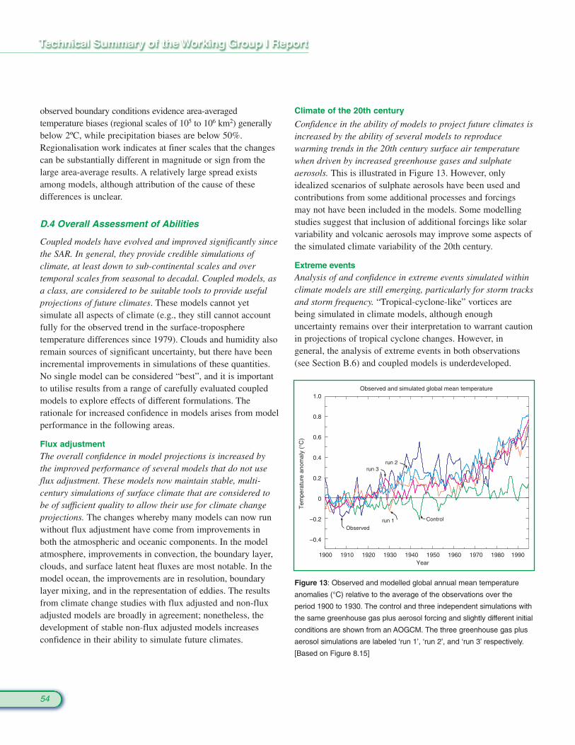
observed boundary conditions evidence area-averagedtemperature biases (regional scales of 105 to 106 km2) generallybelow 2ºC, while precipitation biases are below 50%.Regionalisation work indicates at finer scales that the changescan be substantially different in magnitude or sign from thelarge area-average results. A relatively large spread existsamong models, although attribution of the cause of thesedifferences is unclear.

D.4 Overall Assessment of Abilities

Coupled models have evolved and improved significantly sincethe SAR. In general, they provide credible simulations ofclimate, at least down to sub-continental scales and overtemporal scales from seasonal to decadal. Coupled models, asa class, are considered to be suitable tools to provide usefulprojections of future climates. These models cannot yetsimulate all aspects of climate (e.g., they still cannot accountfully for the observed trend in the surface-tropospheretemperature differences since 1979). Clouds and humidity alsoremain sources of significant uncertainty, but there have beenincremental improvements in simulations of these quantities.No single model can be considered “best”, and it is importantto utilise results from a range of carefully evaluated coupledmodels to explore effects of different formulations. Therationale for increased confidence in models arises from modelperformance in the following areas.

Flux adjustmentThe overall confidence in model projections is increased bythe improved performance of several models that do not useflux adjustment. These models now maintain stable, multi-century simulations of surface climate that are considered tobe of sufficient quality to allow their use for climate changeprojections. The changes whereby many models can now runwithout flux adjustment have come from improvements inboth the atmospheric and oceanic components. In the modelatmosphere, improvements in convection, the boundary layer,clouds, and surface latent heat fluxes are most notable. In themodel ocean, the improvements are in resolution, boundarylayer mixing, and in the representation of eddies. The resultsfrom climate change studies with flux adjusted and non-fluxadjusted models are broadly in agreement; nonetheless, thedevelopment of stable non-flux adjusted models increasesconfidence in their ability to simulate future climates.

Climate of the 20th century

Confidence in the ability of models to project future climates isincreased by the ability of several models to reproducewarming trends in the 20th century surface air temperaturewhen driven by increased greenhouse gases and sulphateaerosols. This is illustrated in Figure 13. However, onlyidealized scenarios of sulphate aerosols have been used andcontributions from some additional processes and forcingsmay not have been included in the models. Some modellingstudies suggest that inclusion of additional forcings like solarvariability and volcanic aerosols may improve some aspects ofthe simulated climate variability of the 20th century.

Extreme eventsAnalysis of and confidence in extreme events simulated withinclimate models are still emerging, particularly for storm tracksand storm frequency. “Tropical-cyclone-like” vortices arebeing simulated in climate models, although enoughuncertainty remains over their interpretation to warrant cautionin projections of tropical cyclone changes. However, ingeneral, the analysis of extreme events in both observations(see Section B.6) and coupled models is underdeveloped.

54

Observed and simulated global mean temperature

Tem

pera

ture

ano

mal

y (°

C)

Observed

Control run 1

run 2run 3

1900

–0.4

–0.2

0

0.2

0.4

0.6

0.8

1.0

1910 1920 1930 1940Year

1950 1960 1970 1980 1990

Figure 13: Observed and modelled global annual mean temperature

anomalies (°C) relative to the average of the observations over the

period 1900 to 1930. The control and three independent simulations with

the same greenhouse gas plus aerosol forcing and slightly different initial

conditions are shown from an AOGCM. The three greenhouse gas plus

aerosol simulations are labeled ‘run 1’, ‘run 2’, and ‘run 3’ respectively.

[Based on Figure 8.15]

Interannual variabilityThe performance of coupled models in simulating ENSO hasimproved; however, its variability is displaced westward andits strength is generally underestimated. When suitablyinitialised with surface wind and sub-surface ocean data, somecoupled models have had a degree of success in predictingENSO events.

Model intercomparisonsThe growth in systematic intercomparisons of models providesthe core evidence for the growing capabilities of climatemodels. For example, the Coupled Model IntercomparisonProject (CMIP) is enabling a more comprehensive andsystematic evaluation and intercomparison of coupled modelsrun in a standardised configuration and responding tostandardised forcing. Some degree of quantification ofimprovements in coupled model performance has now beendemonstrated. The Palaeoclimate Model IntercomparisonProject (PMIP) provides intercomparisons of models for themid-Holocene (6,000 years before present) and for the LastGlacial Maximum (21,000 years before present). The ability ofthese models to simulate some aspects of palaeoclimates,compared to a range of palaeoclimate proxy data, givesconfidence in models (at least the atmospheric component)over a range of difference forcings.

E. The Ident i f icat ion of a HumanInf luence on Cl imate Change

Sections B and C characterised the observed past changes inclimate and in forcing agents, respectively. Section D examinedthe capabilities of climate models to predict the response of theclimate system to such changes in forcing. This Section usesthat information to examine the question of whether a humaninfluence on climate change to date can be identified.

This is an important point to address. The SAR concluded that“the balance of evidence suggests that there is a discerniblehuman influence on global climate”. It noted that the detectionand attribution of anthropogenic climate change signals will beaccomplished through a gradual accumulation of evidence. TheSAR also noted uncertainties in a number of factors, includinginternal variability and the magnitude and patterns of forcingand response, which prevented them from drawing a strongerconclusion.

E.1 The Meaning of Detect ion andAttr ibut ion

Detection is the process of demonstrating that an observedchange is significantly different (in a statistical sense) than canbe explained by natural variability. Attribution is the process ofestablishing cause and effect with some defined level ofconfidence, including the assessment of competing hypotheses.The response to anthropogenic changes in climate forcing occursagainst a backdrop of natural internal and externally forcedclimate variability. Internal climate variability, i.e., climatevariability not forced by external agents, occurs on all time-scalesfrom weeks to centuries and even millennia. Slow climatecomponents, such as the ocean, have particularly important roleson decadal and century time-scales because they integrateweather variability. Thus, the climate is capable of producinglong time-scale variations of considerable magnitude withoutexternal influences. Externally forced climate variations (signals)may be due to changes in natural forcing factors, such as solarradiation or volcanic aerosols, or to changes in anthropogenicforcing factors, such as increasing concentrations of greenhousegases or aerosols. The presence of this natural climate variabilitymeans that the detection and attribution of anthropogenic climatechange is a statistical “signal to noise” problem. Detectionstudies demonstrate whether or not an observed change is highlyunusual in a statistical sense, but this does not necessarily

55

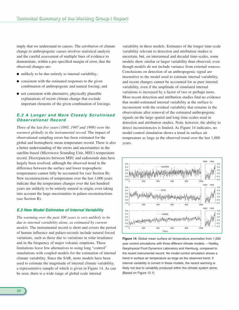
imply that we understand its causes. The attribution of climatechange to anthropogenic causes involves statistical analysisand the careful assessment of multiple lines of evidence todemonstrate, within a pre-specified margin of error, that theobserved changes are:

� unlikely to be due entirely to internal variability;

� consistent with the estimated responses to the givencombination of anthropogenic and natural forcing; and

� not consistent with alternative, physically plausibleexplanations of recent climate change that excludeimportant elements of the given combination of forcings.

E.2 A Longer and More Closely Scrut inisedObservat ional Record

Three of the last five years (1995, 1997 and 1998) were thewarmest globally in the instrumental record. The impact ofobservational sampling errors has been estimated for theglobal and hemispheric mean temperature record. There is alsoa better understanding of the errors and uncertainties in thesatellite-based (Microwave Sounding Unit, MSU) temperaturerecord. Discrepancies between MSU and radiosonde data havelargely been resolved, although the observed trend in thedifference between the surface and lower tropospheric temperatures cannot fully be accounted for (see Section B).New reconstructions of temperature over the last 1,000 yearsindicate that the temperature changes over the last hundredyears are unlikely to be entirely natural in origin, even takinginto account the large uncertainties in palaeo-reconstructions(see Section B).

E.3 New Model Estimates of Internal Variability

The warming over the past 100 years is very unlikely to bedue to internal variability alone, as estimated by currentmodels. The instrumental record is short and covers the periodof human influence and palaeo-records include natural forcedvariations, such as those due to variations in solar irradianceand in the frequency of major volcanic eruptions. Theselimitations leave few alternatives to using long “control”simulations with coupled models for the estimation of internalclimate variability. Since the SAR, more models have beenused to estimate the magnitude of internal climate variability,a representative sample of which is given in Figure 14. As canbe seen, there is a wide range of global scale internal

variability in these models. Estimates of the longer time-scalevariability relevant to detection and attribution studies isuncertain, but, on interannual and decadal time-scales, somemodels show similar or larger variability than observed, eventhough models do not include variance from external sources.Conclusions on detection of an anthropogenic signal areinsensitive to the model used to estimate internal variability,and recent changes cannot be accounted for as pure internalvariability, even if the amplitude of simulated internalvariations is increased by a factor of two or perhaps more.Most recent detection and attribution studies find no evidencethat model-estimated internal variability at the surface isinconsistent with the residual variability that remains in theobservations after removal of the estimated anthropogenicsignals on the large spatial and long time-scales used indetection and attribution studies. Note, however, the ability todetect inconsistencies is limited. As Figure 14 indicates, nomodel control simulation shows a trend in surface airtemperature as large as the observed trend over the last 1,000years.

56

0 200 400 600 800 1000−0.4

−0.2

0.0

0.2

0.4

0.6HadCM2

0 200 400 600 800 1000−0.4

−0.2

0.0

0.2

0.4

0.6

GFDL

0 200 400 600 800 1000

Years

−0.4

−0.2

0.0

0.2

0.4

0.6

HAM3L

1850 1950

−0.4

−0.2

0.0

0.2

0.4

0.6

1850 1950

−0.4

−0.2

0.0

0.2

0.4

0.6

1850 1950

−0.4

−0.2

0.0

0.2

0.4

0.6

Figure 14: Global mean surface air temperature anomalies from 1,000

year control simulations with three different climate models, – Hadley,

Geophysical Fluid Dynamics Laboratory and Hamburg, compared to

the recent instrumental record. No model control simulation shows a

trend in surface air temperature as large as the observed trend. If

internal variability is correct in these models, the recent warming is

likely not due to variability produced within the climate system alone.


E.4 New Est imates of Responses to NaturalForcing

Assessments based on physical principles and modelsimulations indicate that natural forcing alone is unlikely toexplain the recent observed global warming or the observedchanges in vertical temperature structure of the atmosphere.Fully coupled ocean-atmosphere models have usedreconstructions of solar and volcanic forcings over the last oneto three centuries to estimate the contribution of natural forcingto climate variability and change. Although the reconstructionof natural forcings is uncertain, including their effects producesan increase in variance at longer (multi-decadal) time-scales.This brings the low-frequency variability closer to that deducedfrom palaeo-reconstructions. It is likely that the net naturalforcing (i.e., solar plus volcanic) has been negative over thepast two decades, and possibly even the past four decades.Statistical assessments confirm that simulated naturalvariability, both internal and naturally forced, is unlikely toexplain the warming in the latter half of the 20th century (seeFigure 15). However, there is evidence for a detectable volcanicinfluence on climate and evidence that suggests a detectablesolar influence, especially in the early part of the 20th century.Even if the models underestimate the magnitude of theresponse to solar or volcanic forcing, the spatial and temporalpatterns are such that these effects alone cannot explain theobserved temperature changes over the 20th century.

E.5 Sensit iv i ty to Est imates of Cl imateChange Signals

There is a wide range of evidence of qualitative consistenciesbetween observed climate changes and model responses toanthropogenic forcing. Models and observations showincreasing global temperature, increasing land-oceantemperature contrast, diminishing sea-ice extent, glacialretreat, and increases in precipitation at high latitudes in theNorthern Hemisphere. Some qualitative inconsistenciesremain, including the fact that models predict a faster rate ofwarming in the mid- to upper troposphere than is observed ineither satellite or radiosonde tropospheric temperature records.

All simulations with greenhouse gases and sulphate aerosolsthat have been used in detection studies have found that asignificant anthropogenic contribution is required to accountfor surface and tropospheric trends over at least the last 30years. Since the SAR, more simulations with increases in

greenhouse gases and some representation of aerosol effectshave become available. Several studies have included anexplicit representation of greenhouse gases (as opposed to anequivalent increase in CO2). Some have also included tropos-pheric ozone changes, an interactive sulphur cycle, an explicitradiative treatment of the scattering of sulphate aerosols, andimproved estimates of the changes in stratospheric ozone.Overall, while detection of the climate response to these otheranthropogenic factors is often ambiguous, detection of theinfluence of greenhouse gases on the surface temperaturechanges over the past 50 years is robust. In some cases,ensembles of simulations have been run to reduce noise in theestimates of the time-dependent response. Some studies haveevaluated seasonal variation of the response. Uncertainties inthe estimated climate change signals have made it difficult toattribute the observed climate change to one specificcombination of anthropogenic and natural influences, but allstudies have found a significant anthropogenic contribution isrequired to account for surface and tropospheric trends over atleast the last thirty years.

E.6 A Wider Range of Detect ion Techniques

TemperatureEvidence of a human influence on climate is obtained over asubstantially wider range of detection techniques. A majoradvance since the SAR is the increase in the range oftechniques used and the evaluation of the degree to which theresults are independent of the assumptions made in applyingthose techniques. There have been studies using patterncorrelations, optimal detection studies using one or more fixedpatterns and time-varying patterns, and a number of othertechniques. The increase in the number of studies, breadth oftechniques, increased rigour in the assessment of the role ofanthropogenic forcing in climate, and the robustness of resultsto the assumptions made using those techniques, has increasedthe confidence in these aspects of detection and attribution.

Results are sensitive to the range of temporal and spatial scalesthat are considered. Several decades of data are necessary toseparate forced signals from internal variability. Idealisedstudies have demonstrated that surface temperature changes aredetectable only on scales in the order of 5,000 km. Such studiesshow that the level of agreement found between simulationsand observations in pattern correlation studies is close to whatone would expect in theory.

57

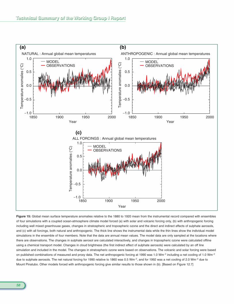
58

ANTHROPOGENIC : Annual global mean temperatures

1850 1900 1950 2000Year

−1.0

−0.5

0.0

0.5

1.0

−1.0

−0.5

0.0

0.5

1.0

Tem

pera

ture

ano

mal

ies

(°C

) MODELOBSERVATIONS

NATURAL : Annual global mean temperatures

1850 1900 1950 2000Year

Tem

pera

ture

ano

mal

ies

(°C

) MODELOBSERVATIONS

MODELOBSERVATIONS

(a) (b)

(c)ALL FORCINGS : Annual global mean temperatures

1850 1900 1950 2000

Year

−1.0

−0.5

0.0

0.5

1.0

Tem

pera

ture

ano

mal

ies

(°C

)

Figure 15: Global mean surface temperature anomalies relative to the 1880 to 1920 mean from the instrumental record compared with ensembles

of four simulations with a coupled ocean-atmosphere climate model forced (a) with solar and volcanic forcing only, (b) with anthropogenic forcing

including well mixed greenhouse gases, changes in stratospheric and tropospheric ozone and the direct and indirect effects of sulphate aerosols,

and (c) with all forcings, both natural and anthropogenic. The thick line shows the instrumental data while the thin lines show the individual model

simulations in the ensemble of four members. Note that the data are annual mean values. The model data are only sampled at the locations where

there are observations. The changes in sulphate aerosol are calculated interactively, and changes in tropospheric ozone were calculated offline

using a chemical transport model. Changes in cloud brightness (the first indirect effect of sulphate aerosols) were calculated by an off line

simulation and included in the model. The changes in stratospheric ozone were based on observations. The volcanic and solar forcing were based

on published combinations of measured and proxy data. The net anthropogenic forcing at 1990 was 1.0 Wm−2 including a net cooling of 1.0 Wm−2

due to sulphate aerosols. The net natural forcing for 1990 relative to 1860 was 0.5 Wm−2, and for 1992 was a net cooling of 2.0 Wm−2 due to

Mount Pinatubo. Other models forced with anthropogenic forcing give similar results to those shown in (b). [Based on Figure 12.7]

59

Most attribution studies find that, over the last 50 years, theestimated rate and magnitude of global warming due toincreasing concentrations of greenhouse gases alone arecomparable with or larger than the observed warming.Attribution studies address the question of “whether themagnitude of the simulated response to a particular forcingagent is consistent with observations”. The use of multi-signaltechniques has enabled studies that discriminate between theeffects of different factors on climate. The inclusion of thetime dependence of signals has helped to distinguish betweennatural and anthropogenic forcings. As more response patternsare included, the problem of degeneracy (differentcombinations of patterns yielding near identical fits to theobservations) inevitably arises. Nevertheless, even with all themajor responses that have been included in the analysis, adistinct greenhouse gas signal remains detectable.Furthermore, most model estimates that take into account bothgreenhouse gases and sulphate aerosols are consistent withobservations over this period. The best agreement betweenmodel simulations and observations over the last 140 years isfound when both anthropogenic and natural factors areincluded (see Figure 15). These results show that the forcingsincluded are sufficient to explain the observed changes, but donot exclude the possibility that other forcings have alsocontributed. Overall, the magnitude of the temperatureresponse to increasing concentrations of greenhouse gases isfound to be consistent with observations on the scalesconsidered (see Figure 16), but there remain discrepiesbetween modelled and observed response to other natural andanthropogenic factors.

Uncertainties in other forcings that have been included do notprevent identification of the effect of anthropogenicgreenhouse gases over the last 50 years. The sulphate forcing,while uncertain, is negative over this period. Changes innatural forcing during most of this period are also estimated tobe negative. Detection of the influence of anthropogenicgreenhouse gases therefore cannot be eliminated either by theuncertainty in sulphate aerosol forcing or because naturalforcing has not been included in all model simulations. Studiesthat distinguish the separate responses to greenhouse gas,sulphate aerosol and natural forcing produce uncertainestimates of the amplitude of the sulphate aerosol and naturalsignals, but almost all studies are nevertheless able to detectthe presence of the anthropogenic greenhouse gas signal in therecent climate record.

The detection and attribution methods used should not besensitive to errors in the amplitude of the global meanresponse to individual forcings. In the signal-estimationmethods used in this report, the amplitude of the signal isestimated from the observations and not the amplitude of thesimulated response. Hence the estimates are independent ofthose factors determining the simulated amplitude of theresponse, such as the climate sensitivity of the model used. Inaddition, if the signal due to a given forcing is estimatedindividually, the amplitude is largely independent of themagnitude of the forcing used to derive the response.Uncertainty in the amplitude of the solar and indirect sulphateaerosol forcing should not affect the magnitude of theestimated signal.

Sea levelIt is very likely that the 20th century warming has contributedsignificantly to the observed sea level rise, through thermalexpansion of sea water and widespread loss of land ice.Within present uncertainties, observations and models are bothconsistent with a lack of significant acceleration of sea levelrise during the 20th century.

E.7 Remaining Uncer taint ies in Detect ionand Attr ibut ion

Some progress has been made in reducing uncertainty, thoughmany of the sources of uncertainty identified in the SAR stillexist. These include:

� Discrepancies between the vertical profile of temperaturechange in the troposphere seen in observations and models.These have been reduced as more realistic forcing historieshave been used in models, although not fully resolved.Also, the difference between observed surface and lower-tropospheric trends over the last two decades cannotbe fully reproduced by model simulations.

� Large uncertainties in estimates of internal climatevariability from models and observations. Although asnoted above, these are unlikely (bordering on very unlikely)to be large enough to nullify the claim that a detectableclimate change has taken place.

� Considerable uncertainty in the reconstructions of solarand volcanic forcing which are based on proxy or limitedobservational data for all but the last two decades.Detection of the influence of greenhouse gases on climate

60

Scaling required on model-simulated signals

−1

0

1

2

G

GS GSIO GSGS GSI

GS GS GS GG

GSIO

S

S

N

So

So

V

Estimated contributions to 20th century warming (°C/century)

−1.0−0.5

0.0

0.5

1.0

1.52.0

G GS GSIOGS GS GSI GS GS GS

G

G

G

SIO

SS

N SoSo V

HadCM

2

HadCM

2

HadCM

3

ECHAM3/

LSG

ECHAM4/

OPYC

ECHAM4/

OPYC

GFDL-R30

CGCM1

CGCM2

HadCM

3

ECHAM3/

LSG

HadCM

2

HadCM

2

HadCM

2

HadCM

3

ECHAM3/

LSG

ECHAM4/

OPYC

ECHAM4/

OPYC

GFDL-R30

CGCM1

CGCM2

HadCM

3

ECHAM3/

LSG

HadCM

2

(a)

(b)

Figure 16: (a) Estimates of the “scaling factors” by which the amplitude of several model-simulated signals must be multiplied to reproduce

the corresponding changes in the observed record. The vertical bars indicate the 5 to 95% uncertainty range due to internal variability. A

range encompassing unity implies that this combination of forcing amplitude and model-simulated response is consistent with the

corresponding observed change, while a range encompassing zero implies that this model-simulated signal is not detectable. Signals are

defined as the ensemble mean response to external forcing expressed in large-scale (>5,000 km) near-surface temperatures over the 1946 to

1996 period relative to the 1896 to 1996 mean. The first entry (G) shows the scaling factor and 5 to 95% confidence interval obtained with the

assumption that the observations consist only of a response to greenhouse gases plus internal variability. The range is significantly less than

one (consistent with results from other models), meaning that models forced with greenhouse gases alone significantly over predict the

observed warming signal. The next eight entries show scaling factors for model-simulated responses to greenhouse and sulphate forcing

(GS), with two cases including indirect sulphate and tropospheric ozone forcing, one of these also including stratospheric ozone depletion

(GSI and GSIO, respectively). All but one (CGCM1) of these ranges is consistent with unity. Hence there is little evidence that models are

61

� Large differences in the response of different models to thesame forcing. These differences, which are often greaterthan the difference in response in the same model with andwithout aerosol effects, highlight the large uncertainties inclimate change prediction and the need to quantifyuncertainty and reduce it through better observational datasets and model improvement.

E.8 Synopsis

In the light of new evidence and taking into account theremaining uncertainties, most of the observed warming overthe last 50 years is likely to have been due to the increase ingreenhouse gas concentrations.

appears to be robust to possible amplification of the solarforcing by ozone-solar or solar-cloud interactions, providedthese do not alter the pattern or time-dependence of theresponse to solar forcing. Amplification of the solar signalby these processes, which are not yet included in models,remains speculative.

� Large uncertainties in anthropogenic forcing are associatedwith the effects of aerosols. The effects of some anthro-pogenic factors, including organic carbon, black carbon,biomass aerosols, and changes in land use, have not beenincluded in detection and attribution studies. Estimates ofthe size and geographic pattern of the effects of theseforcings vary considerably, although individually theirglobal effects are estimated to be relatively small.

systematically over- or under predicting the amplitude of the observed response under the assumption that model-simulated GS signals and

internal variability are an adequate representation (i.e., that natural forcing has had little net impact on this diagnostic). Observed residual

variability is consistent with this assumption in all but one case (ECHAM3, indicated by the asterisk). One is obliged to make this assumption

to include models for which only a simulation of the anthropogenic response is available, but uncertainty estimates in these single signal

cases are incomplete since they do not account for uncertainty in the naturally forced response. These ranges indicate, however, the high

level of confidence with which internal variability, as simulated by these various models, can be rejected as an explanation of recent near-

surface temperature change. A more complete uncertainty analysis is provided by the next three entries, which show corresponding scaling

factors on individual greenhouse (G), sulphate (S), solar-plus-volcanic (N), solar-only (So) and volcanic-only (V) signals for those cases in

which the relevant simulations have been performed. In these cases, multiple factors are estimated simultaneously to account for uncertainty

in the amplitude of the naturally forced response. The uncertainties increase but the greenhouse signal remains consistently detectable. In

one case (ECHAM3) the model appears to be overestimating the greenhouse response (scaling range in the G signal inconsistent with unity),

but this result is sensitive to which component of the control is used to define the detection space. It is also not known how it would respond

to the inclusion of a volcanic signal. In cases where both solar and volcanic forcing is included (HadCM2 and HadCM3), G and S signals

remain detectable and consistent with unity independent of whether natural signals are estimated jointly or separately (allowing for different

errors in S and V responses).

(b) Estimated contributions to global mean warming over the 20th century, based on the results shown in (a), with 5 to 95% confidence

intervals. Although the estimates vary depending on which model's signal and what forcing is assumed, and are less certain if more than one

signal is estimated, all show a significant contribution from anthropogenic climate change to 20th century warming. [Based on Figure 12.12]

62

demographic change, social and economic development,technological change, resource use, and pollutionmanagement. This influence is broadly reflected in thestorylines and resulting scenarios.

Since the SRES was not approved until 15 March 2000, itwas too late for the modelling community to incorporate thefinal approved scenarios in their models and have the resultsavailable in time for this Third Assessment Report. However,draft scenarios were released to climate modellers earlier tofacilitate their input to the Third Assessment Report, inaccordance with a decision of the IPCC Bureau in 1998. Atthat time, one marker scenario was chosen from each of fourof the scenario groups based directly on the storylines (A1B,A2, B1, and B2). The choice of the markers was based onwhich of the initial quantifications best reflected the storylineand features of specific models. Marker scenarios are nomore or less likely than any other scenarios, but areconsidered illustrative of a particular storyline. Scenarioswere also selected later to illustrate the other two scenariogroups (A1FI and A1T) within the A1 family, which specif-ically explore alternative technology developments, holdingthe other driving forces constant. Hence there is anillustrative scenario for each of the six scenario groups, andall are equally plausible. Since the latter two illustrativescenarios were selected at a late stage in the process, theAOGCM modelling results presented in this report only usetwo of the four draft marker scenarios. At present, onlyscenarios A2 and B2 have been integrated by more than oneAOGCM. The AOGCM results have been augmented byresults from simple climate models that cover all sixillustrative scenarios. The IS92a scenario is also presented ina number of cases to provide direct comparison with theresults presented in the SAR.

The final four marker scenarios contained in the SRES differin minor ways from the draft scenarios used for the AOGCMexperiments described in this report. In order to ascertain thelikely effect of differences in the draft and final SRESscenarios, each of the four draft and final marker scenarioswere studied using a simple climate model. For three of thefour marker scenarios (A1B, A2, and B2) temperaturechange from the draft and marker scenarios are very similar.The primary difference is a change to the standardisedvalues for 1990 to 2000, which is common to all thesescenarios. This results in a higher forcing early in the period.

F. The Project ions of the Ear th ’sFuture Cl imate

The tools of climate models are used with future scenarios offorcing agents (e.g., greenhouse gases and aerosols) as inputto make a suite of projected future climate changes thatillustrates the possibilities that could lie ahead. Section F.1provides a description of the future scenarios of forcingagents given in the IPCC Special Report on EmissionScenarios (SRES) on which, wherever possible, the futurechanges presented in this section are based. Sections F.2 toF.9 present the resulting projections of changes to the futureclimate. Finally, Section F.10 presents the results of futureprojections based on scenarios of a future where greenhousegas concentrations are stabilised.

F.1 The IPCC Special Report on EmissionsScenarios (SRES)

In 1996, the IPCC began the development of a new set ofemissions scenarios, effectively to update and replace the well-known IS92 scenarios. The approved new set ofscenarios is described in the IPCC Special Report onEmission Scenarios (SRES). Four different narrativestorylines were developed to describe consistently therelationships between the forces driving emissions and theirevolution and to add context for the scenario quantification.The resulting set of 40 scenarios (35 of which contain dataon the full range of gases required to force climate models)cover a wide range of the main demographic, economic andtechnological driving forces of future greenhouse gas andsulphur emissions. Each scenario represents a specificquantification of one of the four storylines. All the scenariosbased on the same storyline constitute a scenario “family”(See Box 5, which briefly describes the main characteristicsof the four SRES storylines and scenario families). TheSRES scenarios do not include additional climate initiatives,which means that no scenarios are included that explicitlyassume implementation of the United Nations FrameworkConvention on Climate Change or the emissions targets ofthe Kyoto Protocol. However, greenhouse gas emissions aredirectly affected by non-climate change policies designed fora wide range of other purposes (e.g., air quality).Furthermore, government policies can, to varying degrees,influence the greenhouse gas emission drivers, such as

There are further small differences in net forcing, but thesedecrease until, by 2100, differences in temperature change inthe two versions of these scenarios are in the range 1 to 2%.For the B1 scenario, however, temperature change is signifi-cantly lower in the final version, leading to a difference inthe temperature change in 2100 of almost 20%, as a result ofgenerally lower emissions across the full range ofgreenhouse gases.

Anthropogenic emissions of the three main greenhousegases, CO2, CH4 and N2O, together with anthropogenicsulphur dioxide emissions, are shown for the six illustrativeSRES scenarios in Figure 17. It is evident that thesescenarios encompass a wide range of emissions. Forcomparison, emissions are also shown for IS92a. Particularlynoteworthy are the much lower future sulphur dioxideemissions for the six SRES scenarios, compared to the IS92scenarios, due to structural changes in the energy system aswell as concerns about local and regional air pollution.

F.2 Project ions of Future Changes inGreenhouse Gases and Aerosols

Models indicate that the illustrative SRES scenarios lead to verydifferent CO2 concentration trajectories (see Figure 18). By2100, carbon cycle models project atmospheric CO2 concen-trations of 540 to 970 ppm for the illustrative SRES scenarios(90 to 250% above the concentration of 280 ppm in 1750). Thenet effect of land and ocean climate feedbacks as indicated bymodels is to further increase projected atmospheric CO2 concen-trations by reducing both the ocean and land uptake of CO2.These projections include the land and ocean climate feedbacks.Uncertainties, especially about the magnitude of the climatefeedback from the terrestrial biosphere, cause a variation ofabout −10 to +30% around each scenario. The total range is 490to 1260 ppm (75 to 350% above the 1750 concentration).

Measures to enhance carbon storage in terrestrial ecosystemscould influence atmospheric CO2 concentration, but the upperbound for reduction of CO2 concentration by such means is 40

63

Box 5: The EmissionsScenarios of the SpecialRepor t on EmissionsScenarios (SRES)

A1. The A1 storyline and scenariofamily describes a future world of veryrapid economic growth, globalpopulation that peaks in mid-centuryand declines thereafter, and the rapidintroduction of new and more efficienttechnologies. Major underlying themesare convergence among regions,capacity building and increasedcultural and social interactions, with asubstantial reduction in regionaldifferences in per capita income. TheA1 scenario family develops into threegroups that describe alternativedirections of technological change inthe energy system. The three A1groups are distinguished by theirtechnological emphasis: fossilintensive (A1FI), non-fossil energysources (A1T), or a balance across allsources (A1B) (where balanced is

defined as not relying too heavily onone particular energy source, on theassumption that similar improvementrates apply to all energy supply andend-use technologies).

A2. The A2 storyline and scenariofamily describes a very heterogeneousworld. The underlying theme is self-reliance and preservation of localidentities. Fertility patterns acrossregions converge very slowly, whichresults in continuously increasingpopulation. Economic development isprimarily regionally oriented and percapita economic growth and techno-logical change more fragmented andslower than other storylines.

B1. The B1 storyline and scenariofamily describes a convergent worldwith the same global population, thatpeaks in mid-century and declinesthereafter, as in the A1 storyline, butwith rapid change in economic

structures toward a service andinformation economy, with reductionsin material intensity and theintroduction of clean and resource-efficient technologies. The emphasis ison global solutions to economic, socialand environmental sustainability,including improved equity, but withoutadditional climate initiatives.

B2. The B2 storyline and scenariofamily describes a world in which theemphasis is on local solutions toeconomic, social and environmentalsustainability. It is a world withcontinuously increasing globalpopulation, at a rate lower than A2,intermediate levels of economicdevelopment, and less rapid and morediverse technological change than inthe A1 and B1 storylines. While thescenario is also oriented towardsenvironmental protection and socialequity, it focuses on local and regionallevels.

to 70 ppm. If all the carbon released by historic land-usechanges could be restored to the terrestrial biosphere over thecourse of the century (e.g., by reforestation), CO2 concentrationwould be reduced by 40 to 70 ppm. Thus, fossil fuel CO2

emissions are virtually certain to remain the dominant controlover trends in atmospheric CO2 concentration during thiscentury.

Model calculations of the abundances of the primary non-CO2

greenhouse gases by the year 2100 vary considerably across

the six illustrative SRES scenarios. In general A1B, A1T andB1 have the smallest increases, and A1FI and A2, the largest.The CH4 changes from 1998 to 2100 range from −190 to+1970 ppb (−11 to +112%), and N2O increases from +38 to+144 ppb (+12 to +46%) (see Figures 17b and c). The HFCs(134a, 143a, and 125) reach abundances of a few hundred to athousand ppt from negligible levels today. The PFC CF4 isprojected to increase to 200 to 400 ppt, and SF6 is projected toincrease to 35 to 65 ppt.

64

2000 2020 2040 2060 2080 2100

5

10

15

20

25

CO

2 em

issi

ons

(Gt C

)

A1BScenarios

A1TA1FIA2B1B2IS92a

2000 2020 2040 2060 2080 2100

600

800

1000

CH

4 em

issi

ons

(Tg

CH

4)


2000 2020 2040 2060 2080 2100

16

18

20

22

24

26

N2O

em

issi

ons

(Tg

N)


2000 2020 2040 2060 2080 2100

YearYear

50

100

150

SO

2 em

issi

ons

(Tg

S)


Scenarios

Scenarios

Scenarios

Figure 17: Anthropogenic emissions of CO2, CH4, N2O and sulphur dioxide for the six illustrative SRES scenarios, A1B, A2, B1 and B2, A1FI and

A1T. For comparison the IS92a scenario is also shown. [Based on IPCC Special Report on Emissions Scenarios.]

For the six illustrative SRES emissions scenarios, projectedemissions of indirect greenhouse gases (NOx, CO, VOC),together with changes in CH4, are projected to change theglobal mean abundance of the tropospheric hydroxyl radical(OH), by −20% to +6% over the next century. Because of theimportance of OH in tropospheric chemistry, comparable, butopposite sign, changes occur in the atmospheric lifetimes ofthe greenhouse gases CH4 and HFCs. This impact depends inlarge part on the magnitude of and the balance between NOx

and CO emissions. Changes in tropospheric O3 of –12 to +62%are calculated from 2000 until 2100. The largest increasepredicted for the 21st century is for scenarios A1FI and A2and would be more than twice as large as that experiencedsince the Pre-industrial Era. These O3 increases are attributableto the concurrent and large increases in anthropogenic NOx

and CH4 emissions.

The large growth in emissions of greenhouse gases and otherpollutants as projected in some of the six illustrative SRESscenarios for the 21st century will degrade the globalenvironment in ways beyond climate change. Changesprojected in the SRES A2 and A1FI scenarios would degradeair quality over much of the globe by increasing backgroundlevels of tropospheric O3. In northern mid-latitudes duringsummer, the zonal average of O3 increases near the surfaceare about 30 ppb or more, raising background levels to about80 ppb, threatening the attainment of current air qualitystandards over most metropolitan and even rural regions andcompromising crop and forest productivity. This problemreaches across continental boundaries and couples emissionsof NOx on a hemispheric scale.

Except for sulphate and black carbon, models show an approximately linear dependence of the abundance ofaerosols on emissions. The processes that determine theremoval rate for black carbon differ substantially between themodels, leading to major uncertainty in the future projectionsof black carbon. Emissions of natural aerosols such as seasalt, dust, and gas phase precursors of aerosols such asterpenes, sulphur dioxide (SO2), and dimethyl sulphideoxidation may increase as a result of changes in climate andatmospheric chemistry.

The six illustrative SRES scenarios cover nearly the full rangeof forcing that results from the full set of SRES scenarios.Estimated total historical anthropogenic radiative forcingfrom 1765 to 1990 followed by forcing resulting from the six

65


Scenarios


Scenarios


Scenarios

CO

2 co

ncen

trat

ion

(ppm

)

300

4000

3500

3000

2500

N2O

con

cent

ratio

n (p

pb)

CH

4 co

ncen

trat

ion

(ppb

)

2000

1500

500

450

350

400

300

400

500

600

700

800

900

1000

1100

1200

1300

20001980

1980

1980

2020 2040 2060 2080 2100

2000 2020 2040 2060 2080 2100

2000 2020 2040 2060 2080 2100

Figure 18: Atmospheric concentrations of CO2, CH4 and N2O resulting

from the six SRES scenarios and from the IS92a scenario computed

with current methodology. [Based on Figures 3.12 and 4.14]

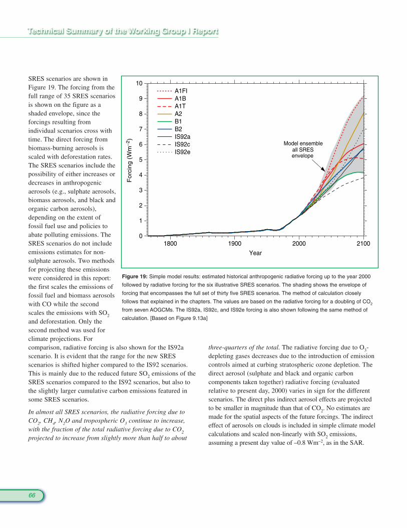
SRES scenarios are shown inFigure 19. The forcing from thefull range of 35 SRES scenariosis shown on the figure as ashaded envelope, since theforcings resulting fromindividual scenarios cross withtime. The direct forcing frombiomass-burning aerosols isscaled with deforestation rates.The SRES scenarios include thepossibility of either increases ordecreases in anthropogenicaerosols (e.g., sulphate aerosols,biomass aerosols, and black andorganic carbon aerosols),depending on the extent offossil fuel use and policies toabate polluting emissions. TheSRES scenarios do not includeemissions estimates for non-sulphate aerosols. Two methodsfor projecting these emissionswere considered in this report:the first scales the emissions offossil fuel and biomass aerosolswith CO while the secondscales the emissions with SO2

and deforestation. Only thesecond method was used forclimate projections. Forcomparison, radiative forcing is also shown for the IS92ascenario. It is evident that the range for the new SRESscenarios is shifted higher compared to the IS92 scenarios.This is mainly due to the reduced future SO2 emissions of theSRES scenarios compared to the IS92 scenarios, but also tothe slightly larger cumulative carbon emissions featured insome SRES scenarios.

In almost all SRES scenarios, the radiative forcing due toCO2, CH4, N2O and tropospheric O3 continue to increase,with the fraction of the total radiative forcing due to CO2

projected to increase from slightly more than half to about

three-quarters of the total. The radiative forcing due to O3-depleting gases decreases due to the introduction of emissioncontrols aimed at curbing stratospheric ozone depletion. Thedirect aerosol (sulphate and black and organic carboncomponents taken together) radiative forcing (evaluatedrelative to present day, 2000) varies in sign for the differentscenarios. The direct plus indirect aerosol effects are projectedto be smaller in magnitude than that of CO2. No estimates aremade for the spatial aspects of the future forcings. The indirecteffect of aerosols on clouds is included in simple climate modelcalculations and scaled non-linearly with SO2 emissions,assuming a present day value of –0.8 Wm−2, as in the SAR.

66

1800 1900 2000 2100

Year

0

1

2

3

4

5

6

7

8

9

10

Fo

rcin

g (

Wm

−2)

A1FIA1BA1TA2B1B2IS92aIS92cIS92e


Figure 19: Simple model results: estimated historical anthropogenic radiative forcing up to the year 2000

followed by radiative forcing for the six illustrative SRES scenarios. The shading shows the envelope of

forcing that encompasses the full set of thirty five SRES scenarios. The method of calculation closely

follows that explained in the chapters. The values are based on the radiative forcing for a doubling of CO2

from seven AOGCMs. The IS92a, IS92c, and IS92e forcing is also shown following the same method of

calculation. [Based on Figure 9.13a]

F.3 Project ions of Future Changes inTemperature

AOGCM results Climate sensitivity is likely to be in the range of 1.5 to 4.5°C.This estimate is unchanged from the first IPCC AssessmentReport in 1990 and the SAR. The climate sensitivity is theequilibrium response of global surface temperature to a doublingof equivalent CO2 concentration. The range of estimates arisesfrom uncertainties in the climate models and their internalfeedbacks, particularly those related to clouds and relatedprocesses. Used for the first time in this IPCC report is theTransient Climate Response (TCR). The TCR is defined as theglobally averaged surface air temperature change, at the time ofdoubling of CO2, in a 1%/yr CO2-increase experiment. This rateof CO2 increase is assumed to represent the radiative forcingfrom all greenhouse gases. The TCR combines elements ofmodel sensitivity and factors that affect response (e.g., oceanheat uptake). The range of the TCR for current AOGCMs is 1.1to 3.1°C.

Including the direct effect of sulphate aerosols reduces globalmean mid-21st century warming. The surface temperatureresponse pattern for a given model, with and without sulphateaerosols, is more similar than the pattern between two modelsusing the same forcing.

Models project changes in several broad-scale climate variables.As the radiative forcing of the climate system changes, the landwarms faster and more than the ocean, and there is greaterrelative warming at high latitudes. Models project a smallersurface air temperature increase in the North Atlantic andcircumpolar southern ocean regions relative to the global mean.There is projected to be a decrease in diurnal temperature rangein many areas, with night-time lows increasing more thandaytime highs. A number of models show a general decrease ofdaily variability of surface air temperature in winter andincreased daily variability in summer in the NorthernHemisphere land areas. As the climate warms, the NorthernHemisphere snow cover and sea-ice extent are projected todecrease. Many of these changes are consistent with recentobservational trends, as noted in Section B.

Multi-model ensembles of AOGCM simulations for a range ofscenarios are being used to quantify the mean climate changeand uncertainty based on the range of model results. For the endof the 21st century (2071 to 2100), the mean change in global

67

average surface air temperature, relative to the period 1961 to1990, is 3.0°C (with a range of 1.3 to 4.5°C) for the A2 draftmarker scenario and 2.2°C (with a range of 0.9 to 3.4°C) for theB2 draft marker scenario. The B2 scenario produces a smallerwarming that is consistent with its lower rate of increased CO2

concentration.

On time-scales of a few decades, the current observed rate ofwarming can be used to constrain the projected response to agiven emissions scenario despite uncertainty in climatesensitivity. Analysis of simple models and intercomparisons ofAOGCM responses to idealised forcing scenarios suggest that,for most scenarios over the coming decades, errors in large-scaletemperature projections are likely to increase in proportion to themagnitude of the overall response. The estimated size of anduncertainty in current observed warming rates attributable tohuman influence thus provides a relatively model-independentestimate of uncertainty in multi-decade projections under mostscenarios. To be consistent with recent observations, anthro-pogenic warming is likely to lie in the range 0.1 to 0.2°C/decadeover the next few decades under the IS92a scenario. This issimilar to the range of responses to this scenario based on theseven versions of the simple model used in Figure 22.

Most of the features of the geographical response in the SRESscenario experiments are similar for different scenarios (seeFigure 20) and are similar to those for idealised 1% CO2-increase integrations. The biggest difference between the 1%CO2-increase experiments, which have no sulphate aerosol, andthe SRES experiments is the regional moderating of the warmingover industrialised areas, in the SRES experiments, where thenegative forcing from sulphate aerosols is greatest. This regionaleffect was noted in the SAR for only two models, but this hasnow been shown to be a consistent response across the greaternumber of more recent models.

It is very likely that nearly all land areas will warm more rapidlythan the global average, particularly those at northern highlatitudes in the cold season. Results (see Figure 21) from recentAOGCM simulations forced with SRES A2 and B2 emissionsscenarios indicate that in winter the warming for all high-latitudenorthern regions exceeds the global mean warming in eachmodel by more than 40% (1.3 to 6.3°C for the range of modelsand scenarios considered). In summer, warming is in excess of40% above the global mean change in central and northern Asia.Only in south Asia and southern South America in June/July/August, and Southeast Asia for both seasons, do the modelsconsistently show warming less than the global average.

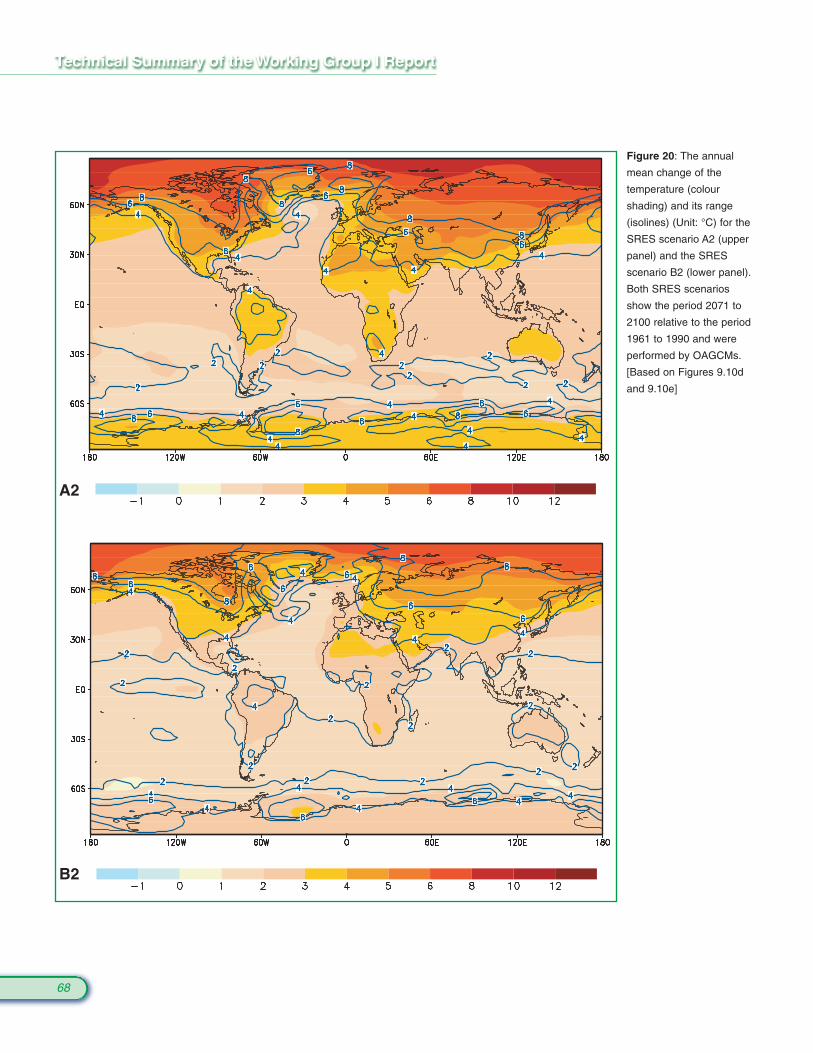
68

A2

B2

Figure 20: The annual

mean change of the

temperature (colour

shading) and its range

(isolines) (Unit: °C) for the

SRES scenario A2 (upper

panel) and the SRES

scenario B2 (lower panel).

Both SRES scenarios

show the period 2071 to

2100 relative to the period

1961 to 1990 and were

performed by OAGCMs.

[Based on Figures 9.10d

and 9.10e]

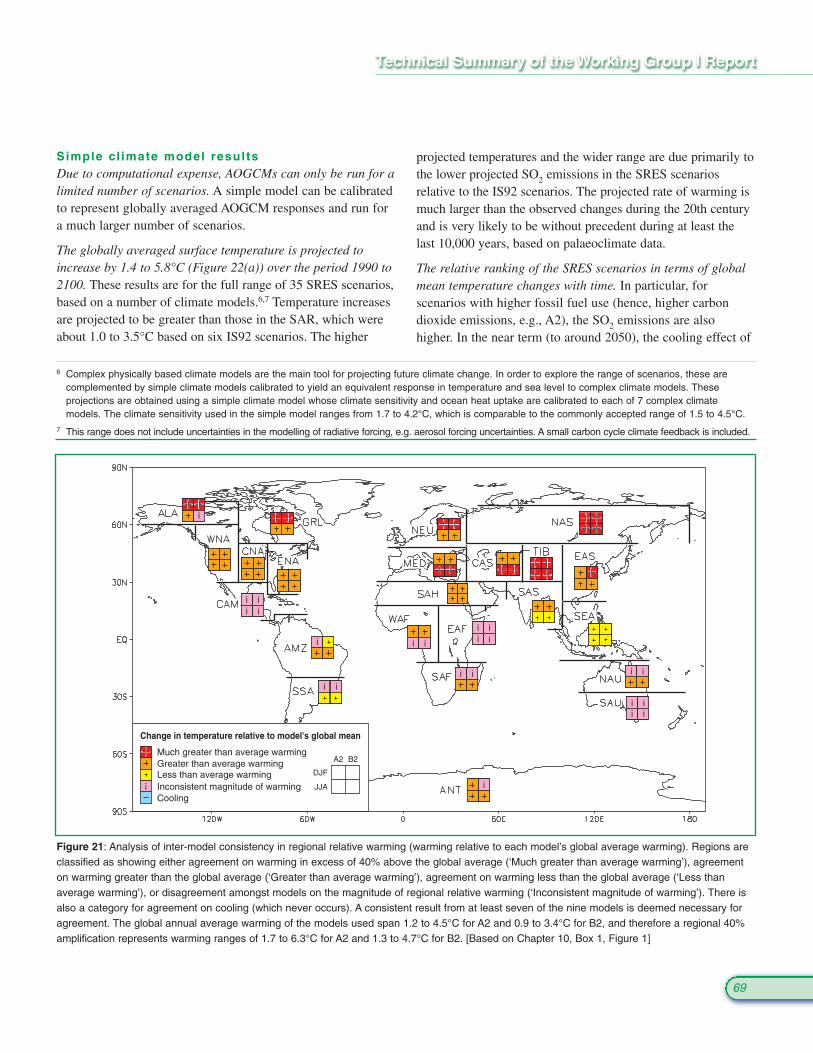
projected temperatures and the wider range are due primarily tothe lower projected SO2 emissions in the SRES scenariosrelative to the IS92 scenarios. The projected rate of warming ismuch larger than the observed changes during the 20th centuryand is very likely to be without precedent during at least thelast 10,000 years, based on palaeoclimate data.

The relative ranking of the SRES scenarios in terms of globalmean temperature changes with time. In particular, forscenarios with higher fossil fuel use (hence, higher carbondioxide emissions, e.g., A2), the SO2 emissions are alsohigher. In the near term (to around 2050), the cooling effect of

69

Simple cl imate model resultsDue to computational expense, AOGCMs can only be run for alimited number of scenarios. A simple model can be calibratedto represent globally averaged AOGCM responses and run fora much larger number of scenarios.

The globally averaged surface temperature is projected toincrease by 1.4 to 5.8°C (Figure 22(a)) over the period 1990 to2100. These results are for the full range of 35 SRES scenarios,based on a number of climate models.6,7 Temperature increasesare projected to be greater than those in the SAR, which wereabout 1.0 to 3.5°C based on six IS92 scenarios. The higher

Change in temperature relative to model's global mean

Much greater than average warmingGreater than average warmingLess than average warmingInconsistent magnitude of warmingCooling

A2 B2

DJF

JJA

ii

i

i

i

i

ii

ii

i ii i

i i

i

iiii

ii

i

Figure 21: Analysis of inter-model consistency in regional relative warming (warming relative to each model’s global average warming). Regions areclassified as showing either agreement on warming in excess of 40% above the global average (‘Much greater than average warming’), agreementon warming greater than the global average (‘Greater than average warming’), agreement on warming less than the global average (‘Less thanaverage warming’), or disagreement amongst models on the magnitude of regional relative warming (‘Inconsistent magnitude of warming’). There isalso a category for agreement on cooling (which never occurs). A consistent result from at least seven of the nine models is deemed necessary foragreement. The global annual average warming of the models used span 1.2 to 4.5°C for A2 and 0.9 to 3.4°C for B2, and therefore a regional 40%amplification represents warming ranges of 1.7 to 6.3°C for A2 and 1.3 to 4.7°C for B2. [Based on Chapter 10, Box 1, Figure 1]

6 Complex physically based climate models are the main tool for projecting future climate change. In order to explore the range of scenarios, these are complemented by simple climate models calibrated to yield an equivalent response in temperature and sea level to complex climate models. These projections are obtained using a simple climate model whose climate sensitivity and ocean heat uptake are calibrated to each of 7 complex climate models. The climate sensitivity used in the simple model ranges from 1.7 to 4.2°C, which is comparable to the commonly accepted range of 1.5 to 4.5°C.

7 This range does not include uncertainties in the modelling of radiative forcing, e.g. aerosol forcing uncertainties. A small carbon cycle climate feedback is included.

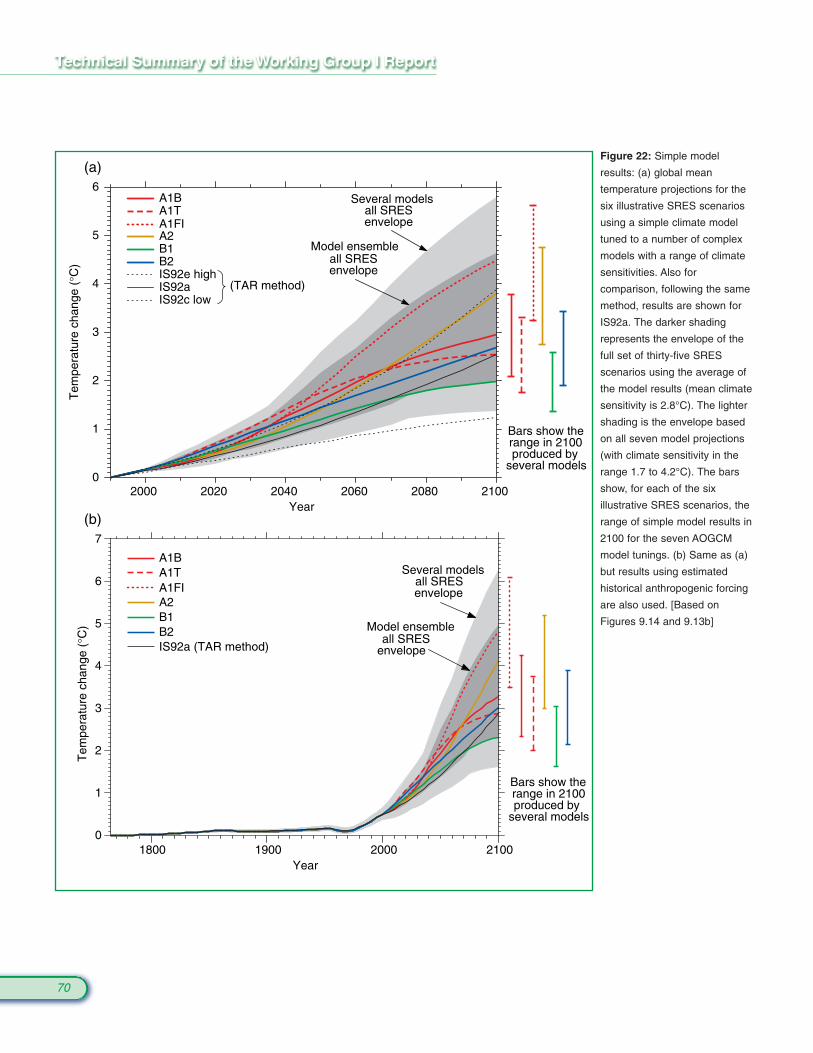
70

2000 2020 2040 2060 2080 2100Year

0

1

2

3

4

5

6

Tem

pera

ture

cha

nge

(°C

)

A1FI

A1BA1T

A2B1B2IS92e highIS92aIS92c low




several models

1800 1900 2000 2100Year

0

1

2

3

4

5

6

7

Tem

pera

ture

cha

nge

(°C

)

A1FI

A1BA1T

A2B1B2IS92a (TAR method)


Model ensembleall SRES

envelope


several models

(b)

(a)

(TAR method)

Figure 22: Simple model

results: (a) global mean

temperature projections for the

six illustrative SRES scenarios

using a simple climate model

tuned to a number of complex

models with a range of climate

sensitivities. Also for

comparison, following the same

method, results are shown for

IS92a. The darker shading

represents the envelope of the

full set of thirty-five SRES

scenarios using the average of

the model results (mean climate

sensitivity is 2.8°C). The lighter

shading is the envelope based

on all seven model projections

(with climate sensitivity in the

range 1.7 to 4.2°C). The bars

show, for each of the six

illustrative SRES scenarios, the

range of simple model results in

2100 for the seven AOGCM

model tunings. (b) Same as (a)

but results using estimated

historical anthropogenic forcing

are also used. [Based on

Figures 9.14 and 9.13b]

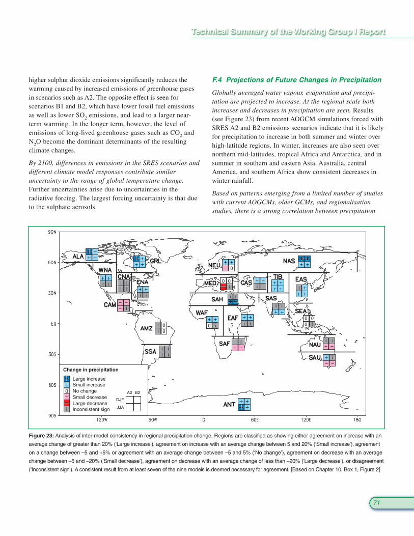
71

F.4 Projections of Future Changes in Precipitation

Globally averaged water vapour, evaporation and precipi-tation are projected to increase. At the regional scale bothincreases and decreases in precipitation are seen. Results(see Figure 23) from recent AOGCM simulations forced withSRES A2 and B2 emissions scenarios indicate that it is likelyfor precipitation to increase in both summer and winter overhigh-latitude regions. In winter, increases are also seen overnorthern mid-latitudes, tropical Africa and Antarctica, and insummer in southern and eastern Asia. Australia, centralAmerica, and southern Africa show consistent decreases inwinter rainfall.

Based on patterns emerging from a limited number of studieswith current AOGCMs, older GCMs, and regionalisationstudies, there is a strong correlation between precipitation

higher sulphur dioxide emissions significantly reduces thewarming caused by increased emissions of greenhouse gasesin scenarios such as A2. The opposite effect is seen forscenarios B1 and B2, which have lower fossil fuel emissionsas well as lower SO2 emissions, and lead to a larger near-term warming. In the longer term, however, the level ofemissions of long-lived greenhouse gases such as CO2 andN2O become the dominant determinants of the resultingclimate changes.

By 2100, differences in emissions in the SRES scenarios anddifferent climate model responses contribute similaruncertainty to the range of global temperature change.Further uncertainties arise due to uncertainties in theradiative forcing. The largest forcing uncertainty is that dueto the sulphate aerosols.

Change in precipitation

A2 B2

DJF

JJA

Large increaseSmall increaseNo change

Inconsistent sign

Small decreaseLarge decrease

i i

i

i

0 00

ii

ii

ii

i

i i

i

i

i

i i

i

i

i

ii

i

i

ii

0

00

00

0

iii

ii

i

0

Figure 23: Analysis of inter-model consistency in regional precipitation change. Regions are classified as showing either agreement on increase with an

average change of greater than 20% (‘Large increase’), agreement on increase with an average change between 5 and 20% (‘Small increase’), agreement

on a change between –5 and +5% or agreement with an average change between –5 and 5% (‘No change’), agreement on decrease with an average

change between –5 and −20% (‘Small decrease’), agreement on decrease with an average change of less than −20% (‘Large decrease’), or disagreement

(‘Inconsistent sign’). A consistent result from at least seven of the nine models is deemed necessary for agreement. [Based on Chapter 10, Box 1, Figure 2]

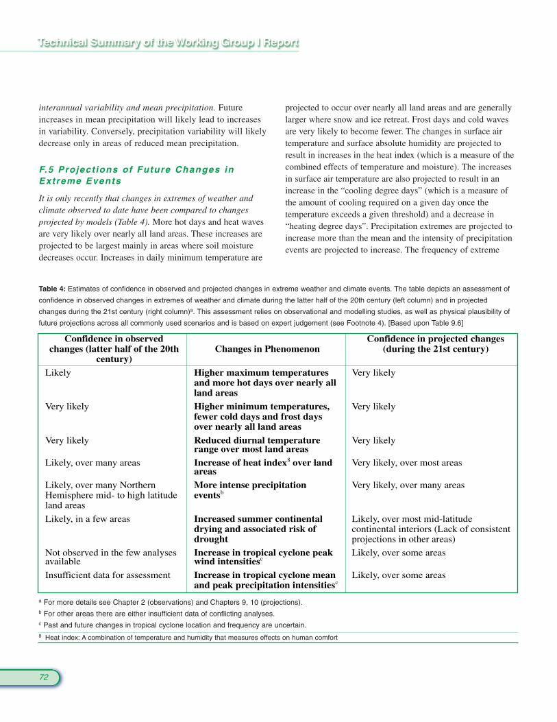
72

projected to occur over nearly all land areas and are generallylarger where snow and ice retreat. Frost days and cold wavesare very likely to become fewer. The changes in surface airtemperature and surface absolute humidity are projected toresult in increases in the heat index (which is a measure of thecombined effects of temperature and moisture). The increasesin surface air temperature are also projected to result in anincrease in the “cooling degree days” (which is a measure ofthe amount of cooling required on a given day once thetemperature exceeds a given threshold) and a decrease in“heating degree days”. Precipitation extremes are projected toincrease more than the mean and the intensity of precipitationevents are projected to increase. The frequency of extreme

interannual variability and mean precipitation. Futureincreases in mean precipitation will likely lead to increasesin variability. Conversely, precipitation variability will likelydecrease only in areas of reduced mean precipitation.

F.5 Project ions of Future Changes inExtreme Events

It is only recently that changes in extremes of weather andclimate observed to date have been compared to changesprojected by models (Table 4). More hot days and heat wavesare very likely over nearly all land areas. These increases areprojected to be largest mainly in areas where soil moisturedecreases occur. Increases in daily minimum temperature are

Confidence in observedchanges (latter half of the 20th

century)Changes in Phenomenon

Confidence in projected changes(during the 21st century)

Likely Higher maximum temperaturesand more hot days over nearly allland areas

Very likely

Very likely Higher minimum temperatures,fewer cold days and frost daysover nearly all land areas

Very likely

Very likely Reduced diurnal temperaturerange over most land areas

Very likely

Likely, over many areas Increase of heat index8 over landareas

Very likely, over most areas

Likely, over many NorthernHemisphere mid- to high latitudeland areas

More intense precipitationeventsb

Very likely, over many areas

Likely, in a few areas Increased summer continentaldrying and associated risk ofdrought

Likely, over most mid-latitudecontinental interiors (Lack of consistentprojections in other areas)

Not observed in the few analysesavailable

Increase in tropical cyclone peakwind intensitiesc

Likely, over some areas

Insufficient data for assessment Increase in tropical cyclone meanand peak precipitation intensitiesc

Likely, over some areas

Table 4: Estimates of confidence in observed and projected changes in extreme weather and climate events. The table depicts an assessment of

confidence in observed changes in extremes of weather and climate during the latter half of the 20th century (left column) and in projected

changes during the 21st century (right column)a. This assessment relies on observational and modelling studies, as well as physical plausibility of

future projections across all commonly used scenarios and is based on expert judgement (see Footnote 4). [Based upon Table 9.6]

a For more details see Chapter 2 (observations) and Chapters 9, 10 (projections).b For other areas there are either insufficient data of conflicting analyses.c Past and future changes in tropical cyclone location and frequency are uncertain.8 Heat index: A combination of temperature and humidity that measures effects on human comfort

73

precipitation events is projected to increase almosteverywhere. There is projected to be a general drying of themid-continental areas during summer. This is ascribed to acombination of increased temperature and potentialevaporation that is not balanced by increases of precipitation.There is little agreement yet among models concerning futurechanges in mid-latitude storm intensity, frequency, andvariability. There is little consistent evidence that showschanges in the projected frequency of tropical cyclones andareas of formation. However, some measures of intensitiesshow projected increases, and some theoretical and modellingstudies suggest that the upper limit of these intensities couldincrease. Mean and peak precipitation intensities from tropicalcyclones are likely to increase appreciably.

For some other extreme phenomena, many of which may haveimportant impacts on the environment and society, there iscurrently insufficient information to assess recent trends, andconfidence in models and understanding is inadequate to makefirm projections. In particular, very small-scale phenomenasuch as thunderstorms, tornadoes, hail, and lightning are notsimulated in global models. Insufficient analysis has occurredof how extra-tropical cyclones may change.

F.6 Project ions of Future Changes inThermohal ine Circulat ion

Most models show weakening of the Northern HemisphereThermohaline Circulation (THC), which contributes to areduction of the surface warming in the northern NorthAtlantic. Even in models where the THC weakens, there is stilla warming over Europe due to increased greenhouse gases. Inexperiments where the atmospheric greenhouse gas concen-tration is stabilised at twice its present day value, the NorthAtlantic THC is projected to recover from initial weakeningwithin one to several centuries. The THC could collapseentirely in either hemisphere if the rate of change in radiativeforcing is large enough and applied long enough. Modelsindicate that a decrease of the THC reduces its resilience toperturbations, i.e., a once reduced THC appears to be lessstable and a shut-down can become more likely. However, it istoo early to say with confidence whether an irreversiblecollapse in the THC is likely or not, or at what threshold itmight occur and what the climate implications could be. Noneof the current projections with coupled models exhibits acomplete shut-down of the THC by 2100. Although the North

Atlantic THC weakens in most models, the relative roles ofsurface heat and fresh water fluxes vary from model to model.Wind stress changes appear to play only a minor role in thetransient response.

F.7 Project ions of Future Changes inModes of Natural Var iabi l i ty

Many models show a mean El Niño-like response in thetropical Pacific, with the central and eastern equatorial Pacificsea surface temperatures projected to warm more than thewestern equatorial Pacific and with a corresponding meaneastward shift of precipitation. Although many models show anEl Niño-like change of the mean state of tropical Pacific seasurface temperatures, the cause is uncertain. It has been relatedto changes in the cloud radiative forcing and/or evaporativedamping of the east-west sea surface temperature gradient insome models. Confidence in projections of changes in futurefrequency, amplitude, and spatial pattern of El Niño events inthe tropical Pacific is tempered by some shortcomings in howwell El Niño is simulated in complex models. Currentprojections show little change or a small increase in amplitudefor El Niño events over the next 100 years. However, even withlittle or no change in El Niño amplitude, global warming islikely to lead to greater extremes of drying and heavy rainfalland increase the risk of droughts and floods that occur with ElNiño events in many regions. It also is likely that warmingassociated with increasing greenhouse gas concentrations willcause an increase of Asian summer monsoon precipitationvariability. Changes in monsoon mean duration and strengthdepend on the details of the emission scenario. The confidencein such projections is limited by how well the climate modelssimulate the detailed seasonal evolution of the monsoons.There is no clear agreement on changes in frequency orstructure of naturally occurring modes of variability, such asthe North Atlantic Oscillation, i.e., the magnitude and characterof the changes vary across the models.

F.8 Project ions of Future Changes in LandIce (Glaciers, Ice Caps and Ice Sheets) ,Sea Ice and Snow Cover

Glaciers and ice caps will continue their widespread retreatduring the 21st century and Northern Hemisphere snow coverand sea ice are projected to decrease further. Methods havebeen developed recently for estimating glacier melt from

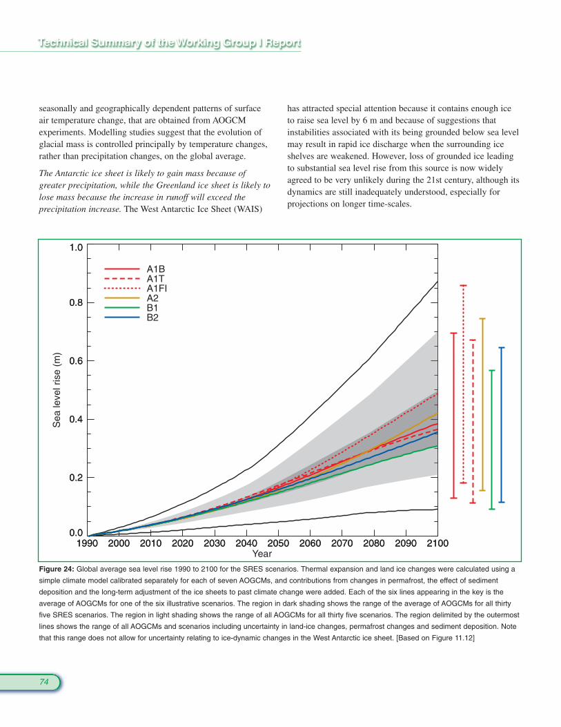
has attracted special attention because it contains enough iceto raise sea level by 6 m and because of suggestions thatinstabilities associated with its being grounded below sea levelmay result in rapid ice discharge when the surrounding iceshelves are weakened. However, loss of grounded ice leadingto substantial sea level rise from this source is now widelyagreed to be very unlikely during the 21st century, although itsdynamics are still inadequately understood, especially forprojections on longer time-scales.

seasonally and geographically dependent patterns of surfaceair temperature change, that are obtained from AOGCMexperiments. Modelling studies suggest that the evolution ofglacial mass is controlled principally by temperature changes,rather than precipitation changes, on the global average.

The Antarctic ice sheet is likely to gain mass because ofgreater precipitation, while the Greenland ice sheet is likely tolose mass because the increase in runoff will exceed theprecipitation increase. The West Antarctic Ice Sheet (WAIS)

74

1990 2000 2010 2020 2030 2040 2050 2060 2070 2080 2090 2100Year

0.0

0.2

0.4

0.6

0.8

1.0

Sea

leve

l ris

e (m

)

1990 2000 2010 2020 2030 2040 2050 2060 2070 2080 2090 21000.0

0.2

0.4

0.6

0.8

1.0

A1B

A1FIA1T

A2B1B2

Figure 24: Global average sea level rise 1990 to 2100 for the SRES scenarios. Thermal expansion and land ice changes were calculated using a

simple climate model calibrated separately for each of seven AOGCMs, and contributions from changes in permafrost, the effect of sediment

deposition and the long-term adjustment of the ice sheets to past climate change were added. Each of the six lines appearing in the key is the

average of AOGCMs for one of the six illustrative scenarios. The region in dark shading shows the range of the average of AOGCMs for all thirty

five SRES scenarios. The region in light shading shows the range of all AOGCMs for all thirty five scenarios. The region delimited by the outermost

lines shows the range of all AOGCMs and scenarios including uncertainty in land-ice changes, permafrost changes and sediment deposition. Note

that this range does not allow for uncertainty relating to ice-dynamic changes in the West Antarctic ice sheet. [Based on Figure 11.12]

F.9 Project ions of Future Changes in SeaLevel

Projections of global average sea level rise from 1990 to2100, using a range of AOGCMs following the IS92ascenario (including the direct effect of sulphate aerosolemissions), lie in the range 0.11 to 0.77 m. This rangereflects the systematic uncertainty of modelling. The maincontributions to this sea level rise are:

� a thermal expansion of 0.11 to 0.43 m, acceleratingthrough the 21st century;

� a glacier contribution of 0.01 to 0.23 m;

� a Greenland contribution of −0.02 to 0.09 m; and

� an Antarctic contribution of −0.17 to +0.02 m.

Also included in the computation of the total change aresmaller contributions from thawing of permafrost,deposition of sediment, and the ongoing contributions fromice sheets as a result of climate change since the LastGlacial Maximum. To establish the range of sea level riseresulting from the choice of different SRES scenarios,results for thermal expansion and land-ice change fromsimple models tuned to several AOGCMs are used (as inSection F.3 for temperature).

For the full set of SRES scenarios, a sea level rise of 0.09 to0.88 m is projected for 1990 to 2100 (see Figure 24),primarily from thermal expansion and loss of mass fromglaciers and ice caps. The central value is 0.48 m, whichcorresponds to an average rate of about two to four times therate over the 20th century. The range of sea level risepresented in the SAR was 0.13 to 0.94 m based on the IS92scenarios. Despite higher temperature change projections inthis assessment, the sea level projections are slightly lower,primarily due to the use of improved models which give asmaller contribution from glaciers and ice sheets. Ifterrestrial storage continues at its current rates, theprojections could be changed by –0.21 to 0.11 m. For anaverage of the AOGCMs, the SRES scenarios give resultsthat differ by 0.02 m or less for the first half of the 21stcentury. By 2100, they vary over a range amounting to about50% of the central value. Beyond the 21st century, sea levelrise depends strongly on the emissions scenario.

Models agree on the qualitative conclusion that the range ofregional variation in sea level change is substantial

75

compared to global average sea level rise. However,confidence in the regional distribution of sea level changefrom AOGCMs is low because there is little similaritybetween models, although nearly all models project greaterthan average rise in the Arctic Ocean and less than averagerise in the Southern Ocean. Further, land movements, bothisostatic and tectonic, will continue through the 21st centuryat rates that are unaffected by climate change. It can beexpected that by 2100, many regions currently experiencingrelative sea level fall will instead have a rising relative sealevel. Lastly, extreme high water levels will occur withincreasing frequency as a result of mean sea level rise. Theirfrequency may be further increased if storms become morefrequent or severe as a result of climate change.

F.10 Project ions of Future Changes inResponse to CO2 Concentrat ionStabi l isat ion Prof i les

Greenhouse gases and aerosols All of the stabilisation profiles studied require CO2

emissions to eventually drop well below current levels.Anthropogenic CO2 emission rates that arrive at stable CO2

concentration levels from 450 to 1,000 ppm were deducedfrom the prescribed CO2 profiles (Figure 25a). The results(Figure 25b) are not substantially different from thosepresented in the SAR; however, the range is larger, mainlydue to the range of future terrestrial carbon uptake causedby different assumptions in the models. Stabilisation at 450,650 or 1,000 ppm would require global anthropogenicemissions to drop below 1990 levels within a few decades,about a century, or about two centuries, respectively, andcontinue to steadily decrease thereafter. Although there issufficient uptake capacity in the ocean to incorporate 70 to80% of foreseeable anthropogenic CO2 emissions to theatmosphere, this process takes centuries due to the rate ofocean mixing. As a result, even several centuries afteremissions occurred, about a quarter of the increase inconcentration caused by these emissions is still present inthe atmosphere. To maintain constant CO2 concentrationbeyond 2300 requires emissions to drop to match the rate ofcarbon sinks at that time. Natural land and ocean sinks withthe capacity to persist for hundreds or thousands of years aresmall (<0.2 PgC/yr).

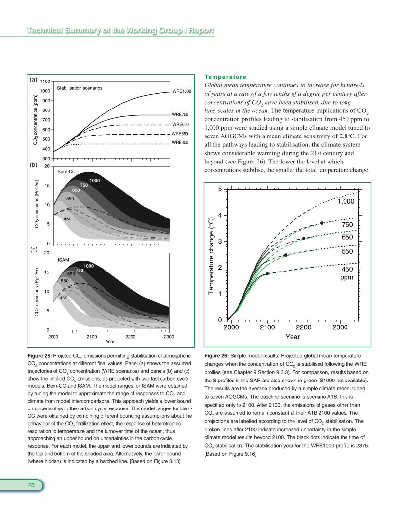
Temperature Global mean temperature continues to increase for hundredsof years at a rate of a few tenths of a degree per century afterconcentrations of CO2 have been stabilised, due to long time-scales in the ocean. The temperature implications of CO2

concentration profiles leading to stabilisation from 450 ppm to1,000 ppm were studied using a simple climate model tuned toseven AOGCMs with a mean climate sensitivity of 2.8°C. Forall the pathways leading to stabilisation, the climate systemshows considerable warming during the 21st century andbeyond (see Figure 26). The lower the level at which concentrations stabilise, the smaller the total temperature change.

76

Figure 25: Projcted CO2 emissions permitting stabilisation of atmosphericCO2 concentrations at different final values. Panel (a) shows the assumedtrajectories of CO2 concentration (WRE scenarios) and panels (b) and (c)show the implied CO2 emissions, as projected with two fast carbon cyclemodels, Bern-CC and ISAM. The model ranges for ISAM were obtainedby tuning the model to approximate the range of responses to CO2 andclimate from model intercomparisons. This approach yields a lower boundon uncertainties in the carbon cycle response. The model ranges for Bern-CC were obtained by combining different bounding assumptions about thebehaviour of the CO2 fertilization effect, the response of heterotrophicrespiration to temperature and the turnover time of the ocean, thusapproaching an upper bound on uncertainties in the carbon cycleresponse. For each model, the upper and lower bounds are indicated bythe top and bottom of the shaded area. Alternatively, the lower bound(where hidden) is indicated by a hatched line. [Based on Figure 3.13]

Year

CO

2 em

issi

ons

(PgC

/yr)

ISAM

CO

2 co

ncen

trat

ion

(ppm

)

Stabilisation scenarios

300

400

500

600

700

800

900

1000

1100

WRE450

WRE550

WRE650

WRE750

WRE1000

CO

2 em

issi

ons

(PgC

/yr)

Bern-CC

450

550

650750

1000

0

5

10

15

20

2000 2100 2200 2300

1000750

650

550

450

0

5

10

15

20

(a)

(b)

(c)

2000 2100 2200 2300Year

0

1

2

3

4

5

Tem

pera

ture

cha

nge

(°C

)

450ppm

550

650

750

1,000

Figure 26: Simple model results: Projected global mean temperature

changes when the concentration of CO2 is stabilised following the WRE

profiles (see Chapter 9 Section 9.3.3). For comparison, results based on

the S profiles in the SAR are also shown in green (S1000 not available).

The results are the average produced by a simple climate model tuned

to seven AOGCMs. The baseline scenario is scenario A1B, this is

specified only to 2100. After 2100, the emissions of gases other than

CO2 are assumed to remain constant at their A1B 2100 values. The

projections are labelled according to the level of CO2 stabilisation. The

broken lines after 2100 indicate increased uncertainty in the simple

climate model results beyond 2100. The black dots indicate the time of

CO2 stabilisation. The stabilisation year for the WRE1000 profile is 2375.


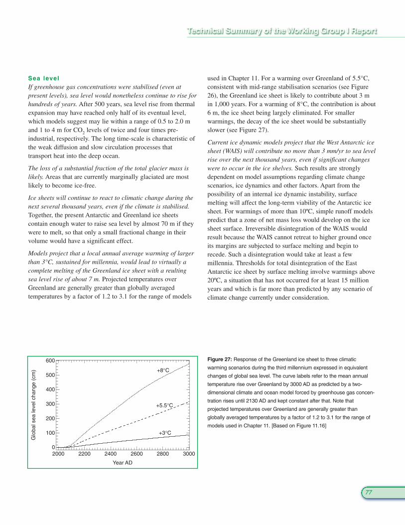
Sea levelIf greenhouse gas concentrations were stabilised (even atpresent levels), sea level would nonetheless continue to rise forhundreds of years. After 500 years, sea level rise from thermalexpansion may have reached only half of its eventual level,which models suggest may lie within a range of 0.5 to 2.0 mand 1 to 4 m for CO2 levels of twice and four times pre-industrial, respectively. The long time-scale is characteristic ofthe weak diffusion and slow circulation processes thattransport heat into the deep ocean.

The loss of a substantial fraction of the total glacier mass islikely. Areas that are currently marginally glaciated are mostlikely to become ice-free.

Ice sheets will continue to react to climatic change during thenext several thousand years, even if the climate is stabilised.Together, the present Antarctic and Greenland ice sheetscontain enough water to raise sea level by almost 70 m if theywere to melt, so that only a small fractional change in theirvolume would have a significant effect.

Models project that a local annual average warming of largerthan 3°C, sustained for millennia, would lead to virtually acomplete melting of the Greenland ice sheet with a reultingsea level rise of about 7 m. Projected temperatures overGreenland are generally greater than globally averagedtemperatures by a factor of 1.2 to 3.1 for the range of models

used in Chapter 11. For a warming over Greenland of 5.5°C,consistent with mid-range stabilisation scenarios (see Figure26), the Greenland ice sheet is likely to contribute about 3 min 1,000 years. For a warming of 8°C, the contribution is about6 m, the ice sheet being largely eliminated. For smallerwarmings, the decay of the ice sheet would be substantiallyslower (see Figure 27).

Current ice dynamic models project that the West Antarctic icesheet (WAIS) will contribute no more than 3 mm/yr to sea levelrise over the next thousand years, even if significant changeswere to occur in the ice shelves. Such results are stronglydependent on model assumptions regarding climate changescenarios, ice dynamics and other factors. Apart from thepossibility of an internal ice dynamic instability, surfacemelting will affect the long-term viability of the Antarctic icesheet. For warmings of more than 10ºC, simple runoff modelspredict that a zone of net mass loss would develop on the icesheet surface. Irreversible disintegration of the WAIS wouldresult because the WAIS cannot retreat to higher ground onceits margins are subjected to surface melting and begin torecede. Such a disintegration would take at least a fewmillennia. Thresholds for total disintegration of the EastAntarctic ice sheet by surface melting involve warmings above20ºC, a situation that has not occurred for at least 15 millionyears and which is far more than predicted by any scenario ofclimate change currently under consideration.

77

600

500

400

300

200

100

0

Glo

bal s

ea le

vel c

hang

e (c

m)

300028002600240022002000

Year AD

+3°C

+5.5°C

+8°C

Figure 27: Response of the Greenland ice sheet to three climatic

warming scenarios during the third millennium expressed in equivalent

changes of global sea level. The curve labels refer to the mean annual

temperature rise over Greenland by 3000 AD as predicted by a two-

dimensional climate and ocean model forced by greenhouse gas concen-

tration rises until 2130 AD and kept constant after that. Note that

projected temperatures over Greenland are generally greater than

globally averaged temperatures by a factor of 1.2 to 3.1 for the range of

models used in Chapter 11. [Based on Figure 11.16]

G. Advancing Understanding

The previous sections have contained descriptions of thecurrent state of knowledge of the climate of the past andpresent, the current understanding of the forcing agents andprocesses in the climate system and how well they can berepresented in climate models. Given the knowledge possessedtoday, the best assessment was given whether climate changecan be detected and whether that change can be attributed tohuman influence. With the best tools available today,projections were made of how the climate could change in thefuture for different scenarios of emissions of greenhouse gases.

This Section looks into the future in a different way.Uncertainties are present in each step of the chain fromemissions of greenhouse gases and aerosols, through to theimpacts that they have on the climate system and society (seeFigure 28). Many factors continue to limit the ability to detect,attribute, and understand current climate change and to projectwhat future climate changes may be. Further work is needed innine broad areas.

G.1 Data

Arrest the decline of observational networks in many parts ofthe world. Unless networks are significantly improved, it maybe difficult or impossible to detect climate change in manyareas of the globe.

Expand the observational foundation for climate studies toprovide accurate, long-term data with expanded temporal andspatial coverage. Given the complexity of the climate systemand the inherent multi-decadal time-scale, there is a need forlong-term consistent data to support climate and environmentalchange investigations and projections. Data from the presentand recent past, climate-relevant data for the last few centuries,and for the last several millennia are all needed. There is aparticular shortage of data in polar regions and data for thequantitative assessment of extremes on the global scale.

G.2 Cl imate Processes and Model l ing

Estimate better future emissions and concentrations ofgreenhouse gases and aerosols. It is particularly important thatimprovements are realised in deriving concentrations fromemissions of gases and particularly aerosols, in addressingbiogeochemical sequestration and cycling, and specifically,and in determining the spatial-temporal distribution of CO2

sources and sinks, currently and in the future.

Understand and characterise more completely dominantprocesses (e.g., ocean mixing) and feedbacks (e.g., fromclouds and sea ice) in the atmosphere, biota, land and oceansurfaces, and deep oceans. These sub-systems, phenomena,and processes are important and merit increased attention toimprove prognostic capabilities generally. The interplay ofobservation and models will be the key for progress. Therapid forcing of a non-linear system has a high prospect ofproducing surprises.

Address more completely patterns of long-term climatevariability. This topic arises both in model calculations and inthe climate system. In simulations, the issue of climate driftwithin model calculations needs to be clarified better in partbecause it compounds the difficulty of distinguishing signaland noise. With respect to the long-term natural variability inthe climate system per se, it is important to understand thisvariability and to expand the emerging capability ofpredicting patterns of organised variability such as ENSO.

Explore more fully the probabilistic character of futureclimate states by developing multiple ensembles of modelcalculations. The climate system is a coupled non-linearchaotic system, and therefore the long-term prediction offuture exact climate states is not possible. Rather the focusmust be upon the prediction of the probability distribution ofthe system’s future possible states by the generation ofensembles of model solutions.

Improve the integrated hierarchy of global and regionalclimate models with emphasis on improving the simulation ofregional impacts and extreme weather events. This will requireimprovements in the understanding of the coupling betweenthe major atmospheric, oceanic, and terrestrial systems, andextensive diagnostic modelling and observational studies thatevaluate and improve simulative performance. A particularlyimportant issue is the adequacy of data needed to attack thequestion of changes in extreme events.

78

79

Socio-economic assumptions(WGII/Ch 3; WGIII/Ch 2 - SRES)

Emissions scenarios(WGIII/Ch 2 - SRES)

Concentration projections(WGI/Ch 3,4,5)

Radiative forcing projections(WGI/Ch 6)

Climate projections(WGI/Ch 8,9,10)

Sea level projections(WGI/Ch 11)

Global change scenarios(WGII/Ch 3)

Inte

ract

ions

and

feed

back

s(W

GI/C

h 3,

4,5,

7; W

GII/

Ch

3)

Impacts(WGII)

Climate scenarios(WGI/Ch 13)

Pol

icy

resp

onse

s: a

dapt

atio

n an

d m

itiga

tion

(WG

II; W

GIII

)

Figure 28: The cascade of uncertainties in projections to beconsidered in developing climate and related scenarios forclimate change impact, adaptation, and mitigation assessment.[Based on Figure 13.2]

G.3 Human Aspects

Link more formally physical climate-biogeochemical modelswith models of the human system and thereby provide the basisfor expanded exploration of possible cause-effect-causepatterns linking human and non-human components of theEarth system. At present, human influences generally aretreated only through emission scenarios that provide externalforcings to the climate system. In future more comprehensivemodels are required in which human activities need to begin tointeract with the dynamics of physical, chemical, andbiological sub-systems through a diverse set of contributingactivities, feedbacks and responses.

G.4 Internat ional Framework

Accelerate internationally progress in understanding climatechange by strengthening the international framework that isneeded to co-ordinate national and institutional efforts so thatresearch, computational, and observational resources may beused to the greatest overall advantage. Elements of thisframework exist in the international programmes supported bythe International Council of Scientific Unions (ICSU), theWorld Meteorological Organization (WMO), the UnitedNations Environment Programme (UNEP), and the UnitedNations Education, Scientific and Cultural Organisation(UNESCO). There is a corresponding need for strengtheningthe co-operation within the international research community,building research capacity in many regions and, as is the goalof this assessment, effectively describing research advances interms that are relevant to decision making.

80

Source Information: TechnicalSummary

This Appendix provides the cross-reference of the topics in theTechnical Summary (page and section) to the sections of thechapters that contain expanded information about the topic.

Sect ion A: Introduct ion

TS Page Technical Summary Section and Topic – Chapter Section

22 A.1 The IPCC and its Working GroupsIntroduction to the Intergovernmental Panel on Climate Change (from the IPCC Secretariat,Geneva) or the IPCC web page at http://www.ipcc.ch

22 − 23 A.2 The First and Second Assessment Reports of Working Group IIPCC, 1990a: Climate Change: The IPCC Scientific Assessment. J.T. Houghton, G.J. Jenkins and J.J. Ephraums (eds.), Cambridge University Press, Cambridge, United Kingdom, 365 pp.

IPCC, 1992: Climate Change 1992: The Supplementary Report to the IPCC Scientific Assessment. J.T. Houghton, B.A. Callander and S.K. Varney (eds.), Cambridge University Press,Cambridge, United Kingdom, 198 pp.

IPCC, 1994: Climate Change 1994: Radiative Forcing of Climate Change and an Evaluation of the IPCC IS92 Emission Scenarios. J.T. Houghton,L.G. Meira Filho, J. Bruce, Hoesung Lee,B.A. Callander, E. Haites, N. Harris and K. Maskell (eds.), Cambridge University Press,Cambridge, United Kingdom, 339 pp.

IPCC, 1996a: Climate Change 1995: The Science of Climate Change. Contribution of Working Group I to the Second Assessment Report of the Intergovernmental Panel on Climate Change [Houghton, J.T., L.G. Meira Filho, B.A. Callander,N Harris, A. Kattenberg, and K. Maskell (eds.)]. Cambridge University Press, Cambridge, United Kingdom and New York, NY, USA, 572 pp.

23 − 24 A.3 The Third Assessment Report: This Technical SummaryBackground to these questions is in Chapter 1.Box 1: What drives changes in climate? – Chapter 1.

Section B:The Observed Changes in the ClimateSystem


26 − 29 B.1 Observed Changes in TemperatureTemperatures in the instrumental record for land and oceans − Chapter 2.2.2 and 2.3.Temperatures above the surface layer from satellite and weather balloon records −Chapter 2.2.3 and 2.2.4.Surface temperatures during the pre-instrumental record from the proxy recordLast 1,000 years − Chapter 2.3.Last glacial and deglaciation − Chapter 2.4.

30 B.2 Observed Changes in Precipitation and Atmospheric MoistureAnnual land-surface precipitation − Chapter 2.5.2.Water vapour − Chapter 2.5.3.Cloud amounts − Chapter 2.5.5.

30 B.3 Observed Changes in Snow Cover and Land- and Sea-Ice ExtentSnow cover and land-ice extent − Chapter 2.2.5.Sea-ice extent − Chapter 2.2.5.Arctic sea-ice thickness − Chapter 2.2.5.

31 − 32 B.4 Observed Changes in Sea LevelChanges During the Instrumental RecordTide gauge data for the 20th century −Chapter 11.3.2.Box 2: What causes sea level to change? −Chapter 11.2.Changes during the pre-instrumental record – Chapter 11.3.1.

32 − 33 B.5 Observed Changes in Atmospheric and Oceanic Circulation PatternsEl Niño-Southern Oscillation (ENSO) −Chapter 2.6.2 and 2.6.3.North Atlantic, Arctic, and Antarctic oscillations −Chapter 2.6.5 and 2.6.6.

33 B.6 Observed Changes in Climate Variability and Extreme Weather and Climate EventsHeavy and extreme precipitation − Chapter 2.7.2. Tropical and extra-tropical storms − Chapter 2.7.3.

33 B.7 The Collective Picture: A Warming World and Other Changes in the Climate SystemA warming world − Chapter 2.8.Little or no change − Chapter 2.2.5 and 2.7.3.

81

Sect ion C: The Forcing Agents That CauseCl imate Change


38 − 43 C.1 Observed Changes in Globally Well-Mixed Greenhouse Gas Concentrations and Radiative Forcing. Carbon dioxide − Chapter 3.2.2, 3.2.3, 3.3.1,3.3.2, and 3.5, Chapter 6.13Methane − Chapter 4.2.1, Chapter 6.13. Nitrous Oxide − Chapter 4.2, Chapter 6.13. Halocarbons and Related Compounds −Chapter 4.2.2, Chapter 6.13.

43 − 44 C.2 Observed Changes in Other Radiatively Important Gases Atmospheric ozone − Chapter 4.2.2 and 4.2.4,Chapter 6.13. Gases with only indirect radiative influence −Chapter 4.2.3, Chapter 6.13

44 − 45 C.3 Observed and Modelled Changes in AerosolsObserved and modelled changes in aerosols −Chapter 5.1, 5.2, 5.3 and 5.4, Chapter 6.7 and 6.8.

45 C.4 Observed Changes in Other Anthropogenic Forcing Agents Land-use (albedo) change − Chapter 6.13.

45 − 46 C.5 Observed and Modelled Changes in Solar ActivityObserved and modelled changes in solar activity -Chapter 6.10.

46 C.6 Global Warming Potentials Global warming potentials - Chapter 6.12

Sect ion D: The Simulat ion of the Cl imateSystem and I ts Changes


46 − 51 D.1 Climate Processes and FeedbacksBox 3: Climate Models: How are they built and how are they applied? − Chapter 8.3.Water vapour − Chapter 7.2.1.Clouds − Chapter 7.2.2 and 7.2.3, Chapter 8.5.1.Stratosphere − Chapter 7.2.4 and 7.2.5,Chapter 8.5.1.Ocean − Chapter 7.3, Chapter 8.5.2.Cryosphere − Chapter 7.5, Chapter 8.5.3.Land surface – Chapter 7.4, Chapter 8.5.4.Carbon cycle − Chapter 3.6.

51 − 53 D.2 The Coupled SystemsModes of natural variability − Chapter 7.6,Chapter 8.7.Box 4: The El Niño/Southern Oscillation (ENSO) − Chapter 7.6.5, Chapter 8.7.1The thermohaline circulation − Chapter 7.3.7 and 7.7, Chapter 9.3.4.Non-linear events and rapid climate change −Chapter 7.7.

53 − 54 D.3 Regionalisation TechniquesCategories of techniques − Chapter 10.1, 10.2,Chapter 13.Coarse resolution AOGCMs − Chapter 10.3,Chapter 13.High resolution RCMs − Chapter 10.5, Chapter 13.

54 − 55 D.4 Overall Assessment of AbilitiesFlux adjustment − Chapter 7.2, 7.3 and 7.6,Chapter 8.4 and 8.9.Climate of the 20th century − Chapter 8.6.Extreme events − Chapter 8.8.Interannual variability − Chapter 8.7.Model intercomparisons − Chapter 8.6.2 and 8.10.

82

Sect ion E: The Ident i f icat ion of a HumanInf luence on Cl imate Change


55 − 56 E.1 The Meaning of Detection and AttributionDetection/Attribution − Chapter 12.1.1 and 12.2.

56 E.2 A Longer and More Closely Scrutinised Observational Record Three of last five years − Chapter 12.2.1.

56 E.3 New Model Estimates of Internal Variability The warming over the past 100 years −Chapter 12.2.2.

57 E.4 New Estimates of Responses to Natural Forcing Natural forcing alone − Chapter 12.2.3.

57 E.5 Sensitivity to Estimates of Climate Changes SignalsResponses to anthropogenic forcing −Chapter 12.2.3.Significant anthropogenic forcing contribution −Chapter 12.2.3.

57 − 59 E.6 A Wider Range of Detection TechniquesTemperature – Chapter 12.3 and 12.4. Sea level – Chapter 11.4.

59 − 61 E.7 Remaining Uncertainties in Detection and AttributionSummary − Chapter 12.5.

61 E.8 Synopsis Most of the observed warming over the past 50 years − Chapter 12.6.

Sect ion F: The Project ions of the Ear th’sFuture Cl imate


62 − 63 F.1 The IPCC Special Report on Emissions Scenarios (SRES)SRES scenarios − Chapter 6.15.2, SRES Report.Box 5: The Emission Scenarios of the Special Report on Emission Scenarios (SRES) −Chapter 6.15.2, SRES Report, Appendix II.

63 − 66 F.2 Projections of Future Changes in Greenhouse Gases and AerosolsCO2 concentration trajectories − Chapter 3.3 and 3.7, Appendix II.Carbon storage in terrestrial ecosystems −Chapter 3.2 and 3.6.Abundance of the non-CO2 greenhouse gases −Chapter 4.3, Chapter 6.15, Appendix II.Emissions of indirect greenhouse gases and atmospheric chemistry − Chapter 4.4.4 and 4.4.5,Chapter 6.15.Emissions of indirect greenhouse gases and air quality – Chapter 4.4.5Dependence of the abundance of aerosols on emissions − Chapter 5.5, Chapter 6.15, Appendix II.Projected aerosol emissions and the SRES scenarios – Chapter 5.5Radiative forcing − Chapter 6.15, Appendix II.

67 − 71 F.3 Projections of Future Changes inTemperature AOGCM Results − Chapter 9.3Simple Climate Model Results − Chapter 9.3

71 − 72 F.4 Projections of Future Changes inPrecipitationGlobally averaged precipitation and variability −Chapter 9.3.

72 − 73 F.5 Projections of Future Changes in Extreme EventsChanges in extreme events − Chapter 9.3.6.

73 F.6 Projections of Future Changes in Thermohaline CirculationWeakening of Thermohaline Circulation −Chapter 9.3.4.

83

73 F.7 Projections of Future Changes in Modes of Natural VariabilityChanges in modes of natural variability −Chapter 9.3.5.

73 − 74 F.8 Projections of Future Changes in Land Ice (Glaciers, Ice Caps and Ice Sheets), Sea Ice and Snow Cover Glaciers, ice caps, and ice sheets − Chapter 11.5.4.

75 F.9 Projections of Future Changes in Sea LevelGlobal average sea level change − Chapter 11.5.1.Regional sea level change − Chapter 11.5.2.Extremes of sea level − Chapter 11.5.3.

75 − 77 F.10 Projections of Future Changes in Response to CO2 Concentration Stabilisation ProfilesGreenhouse gases and aerosols − Chapter 3.7.3.Temperature − Chapter 9.3.3.Sea level − Chapter 11.5.4.

Sect ion G: Advancing Understanding

TS Page Technical Summary Section and Topic −Chapter Section

78 G.1 DataDecline of observational networks and the observing system − Chapter 14.2.1.

78 G.2 Climate Processes and Modelling Greenhouse gases and aerosols − Chapter 14.2.6.Processes − Chapter 14.2.3. Patterns of variability − Chapter 14.2.2.Ensembles of model results − Chapter 14.2.2.Hierarchy of models − Chapter 14.2.2

79 G.3 Human AspectsPhysical system/human system − Chapter 14.3,Chapter 13.1

79 G.4 International FrameworkCo-ordination − Chapter 14.4.

change 2001: t scientific basis

Documents