Challenges in Path Integral Monte Carlo

David Ceperley Physics UIUC

•  Imaginary time path integrals •  Exchange in quantum crystals •  The fermion “sign problem” •  Restricted paths •  The Penalty method •  Quantum dynamics?

Imaginary Time Path Integrals

PIMC Simulations

•  We do Classical Monte Carlo simulations to evaluate averages such as:

•  Quantum mechanically for T>0, we need both to generate the

distribution and do the average:

•  Simulation is possible since the density matrix is positive.

<V >= 1Z

dRV (R)e−βV ( R)∫β = 1/ (kBT ) where R = r1{ ,r2 ,... }

( )( )

1 ( ) ;

; diagonal density matrix

V dRV R RZ

R

ρ β

ρ β

< >=

=

∫

The thermal density matrix •  Find exact many-body

eigenstates of H. •  Probability of

occupying state ϕ is exp(-βEα)

•  All equilibrium properties can be calculated in terms of thermal o-d density matrix

•  Convolution theorem relates high temperature to lower temperature.

2

ˆ-

*

1 2 1 2

1 1

1/

operator notation

off-diagonal density matr

ˆ

( ; ) ( )

ˆ

( , '; ) ( ') ( )

( , '; ) 0 (without statistics)( , ; )

= ' ( , '; )

ix

(

:

E

H

E

kT

H E

R R e

e

R R R R e

R RR R

dR R R

α

α

α α α

βα

α

ββ

βα α

α

β

φ φ

ρ β φ

ρ

ρ β φ φ

ρ βρ β β

ρ β ρ

−

−

=

=

=

=

=

≥+ =

∑

∑

1 2 1 2

2 2

ˆ ˆ ˆ-( ) - -or with operators

', ; )

: H H H

R R

e e eβ β β β

β+ =

∫

Trotter’s formula (1959) •  We can use the effects of operators separately as long as we take small enough time steps. •  n is number of time slices. •  τ is the “time-step”

•  We now have to evaluate the density matrix for potential and kinetic matrices by themselves:

•  Do by FT’s

•  V is “diagonal”

•  Error at finite n comes from commutator

ρ = e−β (T+V )

ρ = limn→∞ e−τ Te−τV⎡⎣

⎤⎦

n

τ = β / n

r e−τ T r ' = 4πλτ( )−3/2e− r−r '( )2 /4λτ

r e−τ V r ' = δ (r − r ')e−τV (r )

2ˆ ˆ,

2T V

eτ ⎡ ⎤− ⎣ ⎦

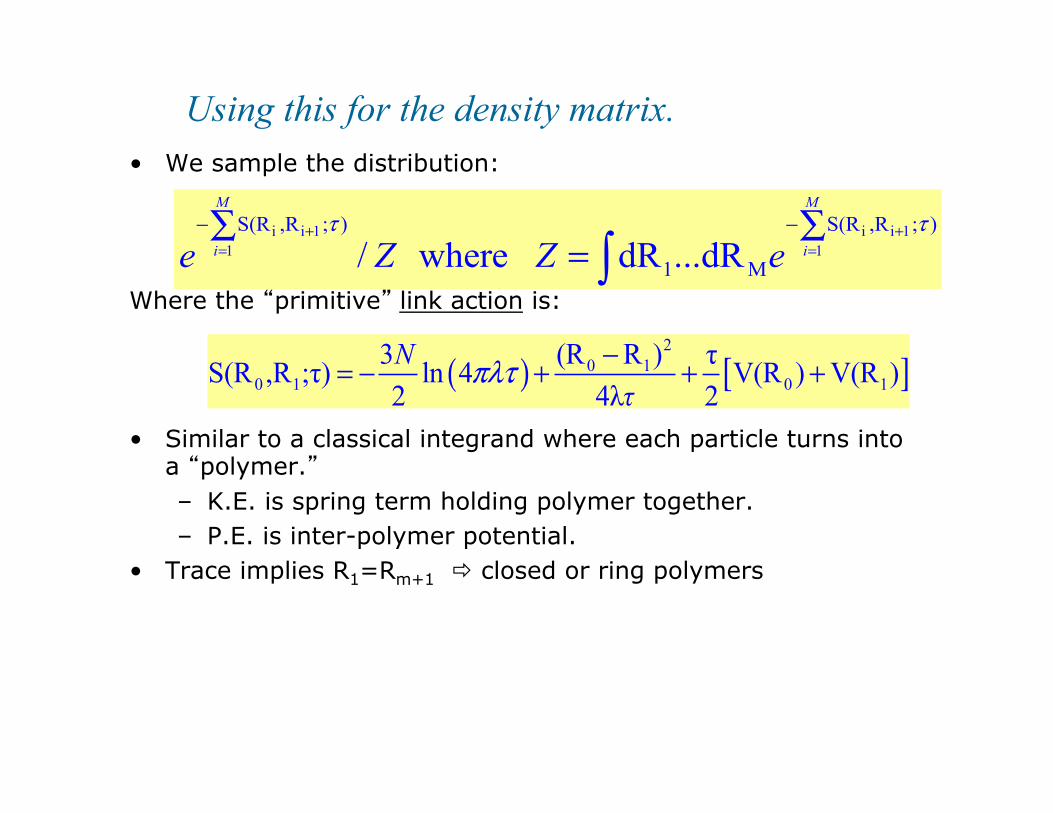
•  We sample the distribution:

Where the “primitive” link action is:

•  Similar to a classical integrand where each particle turns into a “polymer.” –  K.E. is spring term holding polymer together. –  P.E. is inter-polymer potential.

•  Trace implies R1=Rm+1 ð closed or ring polymers

i i 1 i i 11 1

S(R ,R ; ) S(R ,R ; )

1 M/ where dR ...dR

M M

i ie Z Z eτ τ+ +

= =

− −∑ ∑= ∫

( ) [ ]2

0 10 1 0 1

(R R )3 τS(R ,R ;τ) ln 4 V(R ) V(R )2 4λ 2N

τπλτ −= − + + +

Using this for the density matrix.

“Distinguishable” particles •  Each atom is a ring

polymer; an exact representation of a quantum wavepacket in imaginary time.

•  Trace picture of 2D helium. The dots represent the “start” of the path. (but all points are equivalent)

•  The lower the real temperature, the longer the “string” and the more spread out the wavepacket.

Quantum statistics •  For quantum many-body problems, not all states are allowed:

–  Only totally symmetric or antisymmetric (under particle interchange) are allowed. –  Statistics are the origin of BEC, superfluidity, lambda transition, chemistry, materials properties,...

•  Use permutation operator to project out the correct states:

•  Means the path closes on itself with a permutation. R1=PRM+1 •  Too many permutations to sum over; we must sample them. •  PIMC task: sample path { R1,R2,…RM and P} with Metropolis Monte Carlo (MCMC)

using “action”, S, to accept/reject. •  Boson sampling is well-defined since integrand is non-negative

P f (R) = ±( )p

N !p=1

N!

∑ f (PR)

Z = 1N !

p=1

N!

∑ dR1∫ ...dR M ±1( )pe− S(Ri ,Ri+1)

i=1

M

∑

Exchange picture •  Average by

sampling over all paths and over connections.

•  Trial moves involve reconnecting paths differently.

•  At the superfluid transition a “macroscopic” permutation appears.

•  This is reflection of bose condensation within PIMC.

Main Numerical Issues of PIMC •  How to choose the action. We don’t have to use the

primitive form. Higher order forms cut down on the number of slices by a factor of 10. We can solve the 2-body problem exactly.

•  How to sample the paths and the permutations. Single slice moves are too slow. We move several slices at once. Permutation moves are made by exchanging 2 or more endpoints.

•  How to calculate properties. There are often several ways of calculating properties such as the energy.

If you use the simplest algorithm, your code will run 100s or 1000s of times slower than necessary.

Calculations of 3000 He atoms can be done on a workstation-- if you are patient.

Details see: RMP 67, 279 1995.

One sampling method: bisection 1. Select time slices

0

ß

3. Sample midpoints

4. Bisect again, until lowest level

5. Accept or reject entire move

2. Select permutation from possible pairs, triplets, from:

( , ';4 )R PRρ τ

R’

R

PIMC calculation of exchange frequencies

•  Quantum crystals have large zero point motion but are localized at lattice sites for many (105) vibrations.

•  Magnetic properties result from exchange frequencies. •  Review of Path Integral Monte Carlo calculation ring

exchange frequencies (specialized methods). •  Solve exchange Hamiltonian by exact diagonalization of spin

Hamiltonian •  Consider:

B. Bernu (University of Paris) L. Candido (University of Goiania, Brazil) DMC (University of Illinois Urbana-Champaign)

( )2

2 ˆ ˆ ˆ ( ) 12

PP

PiH V R

mH J Pσ= − = − −∇ + ∑∑ →h

3He bcc 3d hcp 3d hex 2d 4He hcp 3d e- Wigner bcc 3d hex 2d

Symmetric double well in imaginary time •  Consider a single particle inside of a double

sphere •  Localization is caused by kinetic energy not

potential, as happens in solid helium. (Potential is not strong enough to keep atoms near the minimum of the potential energy.)

•  Exchange happens rarely but very fast (an instanton is confined in imaginary time). (order 0.2/K)

•  Exchange frequency in imaginary time (used in Path Integrals) is proportional to that in real time.

x

β

Acceptance ratio method •  Let state space consist of path variables AND a single bit

•  For ergodicity we need moves that change σ. Then

•  We don’t actually move back and forth, but perform 2 simulations (A run and B run) and estimate the 2 rates.

•  We only need to perform the simulation at a single beta if we keep track of the exchange time.

1 "B run"

1 "A run"M

M

R PZR Z

σ=+⎧

= ⎨ =−⎩

( ) ( )( )

( )( ) ( )0

Pr 1 Pr 1 1Pr 1 Pr 1 1P Pf J

σβ β β

σ= − →

= = = −= − → −

Imaginary time

Solid 3He

•  We have calculated (Ceperley & Jacucci PRL 58, 1648, 1987) exchange frequencies in bcc and hcp 3He for 2 thru 6 particle exchanges.

•  PIMC gives convincing support for the empirical multiple exchange model. (Roger, Delrieu and Hetherington)

•  Main problem with MEM: there are too many parameters! But if they are determined with PIMC, they are no longer parameters!

•  Exchanges of 2,3,4,5 and 6 particles are important because of Metro effect. •  Large cancellation of effects of various exchanges leads to a frustrated broken

symmetry ground state (u2d2). •  Agrees with experiment measurements on magnetic susceptibility, specific

heat, magnetic field effects, …. •  System of 2d 3He on graphite is more difficult because of exchange outside the

layers. It has a ferromagnetic-antiferromagnetic transition as a function of coverage and is rather similar to 2D Wigner crystal.

But fermions have the sign Problem The expression for Fermi particles, such as He3, is also easily written down. However, in the case of liquid He3, the effect of the potential is very hard to evaluate quantitatively in an accurate manner. The reason for this is that the contribution of a cycle to the sum over permutations is either positive or negative depending on whether the cycle has an odd or even number of atoms in its length L. At very low temperature, the contributions of cycles such as L=51 and L=52 are very nearly equal but opposite in sign, and therefore they very nearly cancel. It is necessary to compute the difference between such terms, and this requires very careful calculation of each term separately. It is very difficult to sum an alternating series of large terms which are decreasing slowly in magnitude when a precise analytic formula for each term is not available. Progress could be made in this problem if it were possible to arrange the mathematics describing a Fermi system in a way that corresponds to a sum of positive terms. Some such schemes have been tried, but the resulting terms appear to be much too hard to evaluate even qualitatively. The (explanation) of the superconducting state was first answered in a convincing way by Bardeen, Cooper, and Schrieffer. The path integral approach played no part in their analysis, and in fact has never proved useful for degenerate Fermi systems.

Feynman and Hibbs,1965.

General statement of the “fermion sign problem”

•  Given a system with N fermions and a known Hamiltonian and a property O (usually the energy): –  How much time T will it take to estimate O to an accuracy ε? –  How does T scale with N and ε?

•  If you can map the quantum system onto an equivalent problem in classical statistical mechanics then:

2NT −∝ εα With 0 <α < 3 This would be a “solved” quantum problem! • All approximations must be controlled! • Algebraic scaling in N! e.g. properties of Boltzmann or Bose systems in equilibrium.

This is one of the most important problems in computation.

“Solved” Quantum Problems •  1-D problems. (simply forbid exchanges) •  Bosons and Boltzmanons at any temperature •  Some lattice models: Heisenberg model, 1/2 filled Hubbard model on bipartite

lattice (Hirsch) with high symmetry. •  Spin symmetric systems with purely attractive interactions: u<0 Hubbard

model, some nuclear models. •  Harmonic oscillators or systems with many symmetries. •  <i|H|j> non-positive in some representation. •  Fermions in special boxes (Kalos)

UNSOLVED: •  Quantum dynamics •  Fermions, for example electrons in materials •  Bosons in special ensembles or with magnetic fields.

Fixed-Node method with PIMC •  Get rid of negative walks by canceling them with positive

walks. We can do this if we know where the density matrix changes sign. Restrict walks to those that stay on the same side of the node.

•  Fixed-node identity. Gives exact solution if we know the places where the density matrix changes sign: the nodes.

•  Classical correspondence exists!! •  Problem: fermion density matrix appears on both sides of the

equation. We need nodes to find the density matrix. •  But still useful approach. (e.g. in classical world we don’t

know V(R) but we still do MD.)

*

( ( ))* 0 *

( , ; ) 0

1( , ; ) ( 1) with =PR !

F t

P S R tF t

P R R t

R R dR e RNβ

ρ

ρ β −

>

= −∑ ∫

Proof of the fixed node method 1.  The density matrix satisfies the Bloch equation with

initial conditions.

2.  One can use more general boundary conditions, not only initial conditions, because solution at the interior is uniquely determined by the exterior-just like the equivalent electrostatic problem.

3.  Suppose someone told us the surfaces where the density matrix vanishes (the nodes). Use them as boundary conditions.

4.  Putting an infinite repulsive potential at the barrier will enforce the boundary condition.

5.  Returning to PI’s, any walk trying to cross the nodes will be killed.

6.  This means that we just restrict path integrals to stay in one region.

( )20

( , ) 1( , ) ( ) ( , ) ( ,0) 1 ( )!

P

P

R t R t V R R t R R PRt N

ρ λ ρ ρ ρ δ∂ = ∇ − = − −∂ ∑

R PR0 R0

β

neg pos neg

The nodes of the density matrix have an imaginary time dependence.

High temperature Low temperature

( )0 0, ; 0 with , fixed.F R R t R tρ =

Can show there are only 2 nodal pockets in many cases.

Group Meeting

Free particle nodes •  For non-interacting (NI) particles the nodes are the finite temperature

version of a Slater determinant:

At high T, nodes are hyperplanes. At low T, nodes minimize the kinetic energy.

Nodes have “time dependence”. •  Problems: no spin-coupling in nodes, no formation of electronic bound

states.

( )( )

( ) ( )2( ')

-3/2 4

1( ', ; ) det ' , ;!

where ' , ; is the single particle density matrix.

', ; = 4 periodic images

NIF i j

i j

r r

R R t g r r tN

g r r t

g r r t e λτ

ρ

πλτ−−

⎡ ⎤= ⎣ ⎦

+

RPIMC with approximate nodes

•  In almost all cases, we do not know the “nodal” surfaces. We must make an ansatz.

•  At low temperature, the nodal condition becomes :ψT(R)=0 as in FN-DMC. •  We get a fermion density matrix (function with the right symmetry) which

satisfies the Bloch equation at all points except at the node. •  There will be a derivative mismatch across the nodal surface unless nodes

are correct. •  In many cases, there is a free energy bound: find the best nodes using the

variational principle.

Other fermion issues

•  Bosonic PIMC methods are applicable! Fermion code is built on top of bosonic code.

•  Reference point moves are expensive: all slices must be checked for nodal violations (not needed for ground state nodes)

•  We observe a “glass transition” of the paths at low temperature. Algorithm is not practically ergodic for T<<TF!

•  Permutations are still needed! However, 2 particle exchanges will always be rejected. Only odd particle cyclic exchanges (3,5,…) allowed as updates.

•  We need fast methods to determine good “nodal” actions. •  Computing the fermion density matrix is O(N3). We have done ~500

electrons. Larger system require sparse matrix methods.

Regimes for Quantum Monte Carlo dense hydrogen

Diffusion Monte Carlo

RPIM

C

CEIMC

Coupled Electron-Ionic Monte Carlo:CEIMC

1.  Do Path Integrals for the ions at T>0. 2.  Let electrons be at zero temperature, a reasonable approximation for

room temperature simulations. (Born-Oppenheimer approx.) 3.  Use Metropolis MC to accept/reject moves based on QMC

computation of electronic energy

. electrons

ions

R

S èS*

The “noise” coming from electronic energy can be treated without approximation using the penalty method.

The Penalty method DMC & Dewing, J. Chem. Phys. 110, 9812(1998).

•  Assume estimated energy difference Δe is normally distributed* with variance σ2 and the correct mean.

< Δe > = ΔE < [Δe- ΔE]2 > = σ2

*central limit thrm applies since we average over many steps

•  a(Δe; σ) is acceptance ratio. •  average acceptance A(ΔE) = < a(Δe) > •  We can achieve detailed balance: A(ΔE) =exp (-ΔE )A(-ΔE) if

we accept using: a(x, σ) = min [ 1, exp(-x- σ2/2)] •  σ2/2 is “penalty” . Causes extra rejections. •  Large noise (order kBT) is more efficient than low noise,

because the QMC will then be faster.

Problem with time dependent correlations •  The imaginary time path integral method can calculate

equilibrium static properties of quantum systems. •  Real time behavior presents another difficult sign problem •  Direct real-time dynamics (exp(-itH)) is VERY difficult

for interesting values of “t”. •  An easier dynamics: How does a quantum system in

equilibrium respond to a weak, time dependent probe? •  “linear response” accounts for conductivity, optical

properties, diffusion,… •  For a probe “A”, and a response “B” the formula is:

SAB ω( ) = Z −1 dt

−∞

∞

∫ eiωt B*e− itH Ae− β−it( )H

Imaginary time correlations •  With PIMC we can calculate imaginary time dynamics:

If we could determine this analytically we could just substitute imaginary

values for real values. •  Dynamic structure function is the response to a density perturbation is

(e.g. density-density response, A and B are FT of density)

•  Sk(ω) is measured by neutron scattering. We want to invert the

“Laplace transform” to get Sk(ω) .

FAB τ( ) = Z −1 Be−τ H Ae− β−τ( )H

Sk (ω ) = 12π

dt−∞

∞

∫ eiωt Fk (t) where O = 1N

eik ⋅ri

i=1

N

∑

Fk (τ ) = dω−∞

∞

∫ e−τωSk (ω )

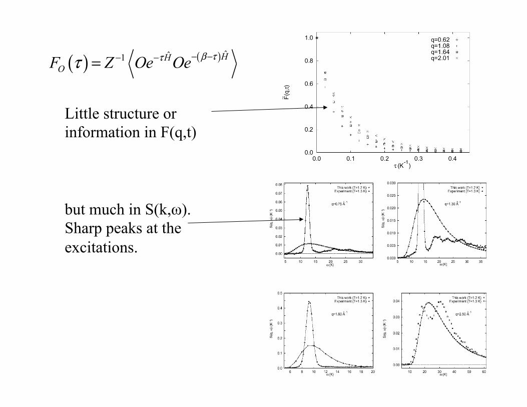
Little structure or information in F(q,t) but much in S(k,ω). Sharp peaks at the excitations.

( ) ( ) ˆˆ1 HHOF Z Oe Oe β τττ − −− −=

Bayes’ theorem •  What is the most probable value of Sk(ω) given:

–  The PIMC data –  Prior knowledge of Sk(ω)?

•  Bayes’ theorem •  Likelihood function follows from central limit theorem:

•  But what to choose for the prior Pp(S(ω))? Typical choice is the “entropy.”

Pr S(ω) F(t)( ) ∝ PL

F(t) S(ω)( )PP(S(ω))

PL

F(t) S(ω)( ) ∝ exp −12

δF(τ)σ τ ,τ '( )−1 δF(τ ')τ ,τ '∑

⎡

⎣⎢

⎤

⎦⎥

δF(τ) = F τ( ) − F τ( ) and σ τ ,τ '( ) = δF τ( )δF τ '( )

( ) ( ) ( )( )ω

ω α ω ω ω⎡ ⎤∝ ⎢ ⎥⎣ ⎦∑( ( )) exp ln /PP S S S m

Now two routes to making the inversion: 1.  Sample Sk(ω). AvEnt Using MCMC make moves in Sk(ω)

space. Take averages and also get idea of the allowed fluctuations. Model defined self consistently

2.  Find most probable Sk(ω). MaxEnt Maximize function. Ok if the p.d.f. is highly peaked. Estimate errors by the curvature at the maximum. Fast to do numerically but makes more assumptions. How do we choose α? Choose it from its own prior function so the strength of the likelihood function and the prior function are balanced. P(α)=1/ α.

Example: Liquid 4He Boninsegni and DMC

•  Calculate Fk(t) using PIMC. •  AvEnt works beautifully in normal phase. •  Gives peaks too broad in the superfluid phase. Failure of

the entropic prior. •  It makes the assumption that energy modes are uncoupled.

This is false! Energy levels repel each other so that if there is energy at one level, it is unlikely at nearby values.

•  Would require incredible precision to get sharp features. •  But good method for determining the excitation energy.

Comparison in normal liquid He phase

•  MaxEnt works well in normal phase (T=4K)

•  Modes are quantum but independent of each other

Comparison in Superfluid

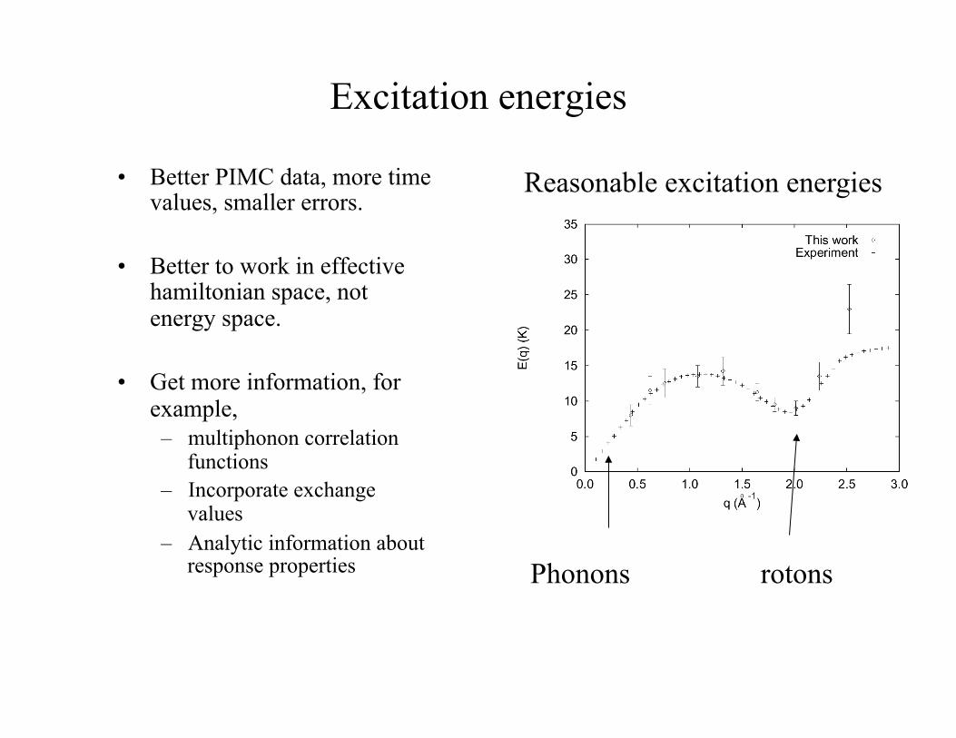
Excitation energies

•  Better PIMC data, more time values, smaller errors.

•  Better to work in effective hamiltonian space, not energy space.

•  Get more information, for example, –  multiphonon correlation

functions –  Incorporate exchange

values –  Analytic information about

response properties

Reasonable excitation energies

Phonons rotons

Dictionary of the Quantum-Classical Isomorphism

Quantum Classical Bose condensation Delocalization of ends Boson statistics Joining of polymers Exchange frequency Free energy to link

polymers Free energy Free energy Imaginary velocity Bond vector Kinetic energy Negative spring energy Momentum distribution FT of end-end

distribution Particle Ring polymer Potential energy Iso-time potential Superfluid state Macroscopic polymer Temperature Polymer length Pauli Principle Restricted Paths Cooper Pairing Paired Fermion Paths Fermi Liquid Winding restricted paths Insulator Nonexchanging paths

Attention: some words have opposite meanings. “fermion dictionary”

•  It is interesting that some quantum many-body systems can be “exactly” modeled with classical simulation methods (i.e. MCMC or MD).

•  What are the boundaries? Which problems are accessible in principle?

•  This is a very important scientific/mathematical problem, i.e. to model matter at the quantum level much more accurately and efficiently.

Review article on PIMC: Rev. Mod. Phys. 67, 279 (1995).