cha pter 6 exp erim en tal sagna c in terfer o met ereandrei/389/sagnac-interferometer-expt.pdf ·...

Chapter 6

Experimental Sagnac

Interferometer

6.1 Experimental Set-Up

The experimental set-up of the Sagnac interferometer is identical to that used

to make transmission measurements (Fig. 4.1 on page 76) up to the optical

fibre. After the pump and probe beams have left the optical fibre, the set-up is

significantly modified to form the Sagnac interferometer, Fig. 5.3 on page 116.

The optical fibre ensures that the pump and probe beams co-propagate.

The Sagnac interferometer is formed by the loop originating at the second beam

splitter (BS2). Probe beams propagate in both directions around the loop,

while the pump beams are coupled out of the loop by the polarizing beam

splitting cube; only the clockwise propagating pump beam passes through the

Rb vapour cell. After completing the loop of the interferometer the two probe

beams interfere on BS2. 50% of the interference propagates towards photodiode

A and 50% towards the first beam splitter (BS1). A neutral density filter (ND)

ensures that only 25% of the output form the interferometer is incident upon

photodiode A. On BS1 the output of the interferometer is divided again such

that 25% of the output of the interferometer is incident upon photodiode B.

In practice the beam splitters do not perform as perfect 50 : 50 beam splitters.

This leads to a small di!erence in the obtained signals from those predicted in

equations 5.62 and 5.63 on the preceding page. This is overcome by making

122

Chapter 6. Experimental Sagnac Interferometer 123

small adjustments to the mechanical slits.

In order to ensure that the two arms of the interferometer counter-propagate, a

Watec high resolution CCD camera (WAT-902B) with a Computar 25 mm lens

was used to monitor the degree of overlap of the beams on the mirrors within

the interferometer. An iterative process — monitoring the overlap on mirror A,

while adjusting mirror B, then monitoring mirror B whilst adjusting mirror A —

allows the beams to be brought very close to counter-propagating. Monitoring

the beams in the two output arms of the interferometer allows the counter-

propagating arms within the interferometer to be brought to be “perfectly”

counter-propagating. When the beams are perfectly counter-propagating and

there is no absorbing medium present in the interferometer output arm B will be

bright, while arm A will be dark — encapsulated in equation 5.42 and equation

5.39, and shown in Fig. 6.1(upper).Arm A Arm B“Perfect”Alignment“Biased”Alignment

Figure 6.1: The output beam profiles for the two arms of the Sagnac inter-

ferometer, for the case of perfectly counter-propagating beams and for the

biased alignment that leads to the dispersion signals. Arm A profiles are

shown on the left and Arm B on the right. The grey rectangles show the

position of the mechanical slits.

A change in the refractive index of the medium for one direction of propagation

shifts the fringe pattern. However the sensitivity is minimal, as the shift is about

a maximum or minimum of the interference pattern, where the rate of change of


(i)

(ii)

(iii)

Figure 6.2: The output beam profiles of the Sagnac interferometer, as

recorded on the Watec CCD camera, for the biased alignment. Arm A is

on the left-hand side while arm B is on the right-hand side. (i) Shows the

profiles before the slits. (ii) The beam profiles as viewed on the slits. (iii)

The beam profiles of the light transmitted through the slits.

intensity with displacement is lowest. To enhance the sensitivity we “bias” the

interferometer by introducing a small angle between the counter-propagating

beams, [99, 101], such that both light and dark fringes appear in the interference

pattern at both outputs, Fig. 6.1(lower) and Fig. 6.2(i). Two mechanical slits

aperture the fringe pattern, such that only the region between the light and

dark fringe is focussed onto the photodiode, Figs. 6.1(lower), 6.2(ii) and (iii).

This biasing technique enables one to obtain maximal sensitivity to changes in

the refractive index and a signal that is directly proportional to the refractive

index di!erence between the two counter-propagating probes, § 5.3. For all


traces recorded with both the pump and probe propagating through the vapour

cell, traces were also recorded with the pump beam blocked before the Sagnac

interferometer. This alignment procedure was adopted so that the probe-only

signal could be subtracted from the pump-and-probe signal — hence allowing

any features in the scan across the resonance that are not due to the presence

of the pump beam to be removed from the spectra.

6.1.1 Photodiode Circuit

In work presented in chapter 4 of this thesis, lock-in amplifiers have been used

to detect the EIT resonances. Concern was raised that the lock-in amplifier

may be limiting the line shape of the transmission resonances, [104]. In order

to avoid the use of a lock-in amplifier, and yet still be able to measure the

EIT resonances it was necessary to use a photodiode circuit with lower noise

levels than that which had previously been used. The photodiode circuit used

+_ RC -9 VOutput0 V+9 V

C

R

Figure 6.3: The photodiode circuit used to measure the output from the

Sagnac interferometer. The op-amp used is either an AD548 or an AD648,

the photodiode is a BPX–65. R is 10 MΩ and C is 4.7 pF.

throughout this chapter is shown in Fig. 6.3. The main di!erence between this

circuit and those used in experiments in previous work in this thesis, is that in

this case the photodiode is not biased. This leads to two main advantages over

the previous circuits, a lesser influence from dark currents, and a wider range

over which the photocurrent is linear with radiant intensity, [40, 41, 105]. The

improvement in signal to noise ratio of this photodiode circuit, over that used

in earlier work in this thesis, was investigated by J. Ga!ney1.

1This work was carried out during a Nuffield funded summer project.


The output voltage of this photodiode circuit has the same form of temporal

filtering as the photodiode circuits used in chapter 4, shown in Fig. 4.9 on

page 86. However with a di!erent value of R = 10 M", the output voltage will

be a factor of 10 higher and will have a frequency cut-o! as shown in Fig. 6.4.

With the impedance decreasing significantly over angular frequencies ! 10 kHz,

it follows that changes in signal on a time scale" 100 µs will be heavily filtered.

2.5

5

7.5

10

0.1 1 10 100

Imped

ance

(M!

)

Angular Frequency (kHz)

Figure 6.4: The output voltage of the photodiode circuit is directly pro-

portional to the output impedance. The calculated output impedance of the

photodiode circuit as a function of angular frequency is shown above, for

R = 10 MΩ and C = 4.7 pF.

6.2 Sagnac Interferometer Experimental Results

6.2.1 Beam Profiles

The profile of the pump and probe beams has a direct a!ect upon the line shape

and width of the EIT features, [68]. In order to determine the beam profiles the

Rb cell was removed from the interferometer and replaced with a 0.25 mm wide

slit. The slit was mounted on a micrometer-driven translation stage, allowing

the slit to be translated perpendicular to the direction of propagation of the

beams. After the beam has passed through the slit it is focussed onto a photo-

diode. The signal recorded on the photodiode is plotted against the position of

the centre of the slit. Typical data for both clockwise and anticlockwise beams


are shown in Fig. 6.5. Both pump and probe beams have circularly-symmetric

0

0.2

0.4

0.6

0.8

1

-3 -2 -1 0 1 2 3

No

rmal

ized

Sig

nal

Displacement from Centre of Beam (mm)

Figure 6.5: The red plots show a typical beam profile for the clockwise

beams: experimental measurements (circles) and Gaussian fit (line) with a

1/e full-width of (1.890 ± 0.007) mm. The blue plots show a typical beam

profile for the anticlockwise beams: experimental measurements (circles) and

Gaussian fit (line) with a 1/e full-width of (3.177 ± 0.003) mm.

Gaussian profiles, as expected from the circular core of the optical fibre, [106],

in agreement with perpendicular sets of beam profile measurements. The an-

ticlockwise beams travel a distance of 2.2 m from the output of the optical

fibre to the slit, whereas the clockwise beams propagate 0.7 m from the fibre

output to the slit. The clockwise pump and probe fields have a 1/e full-width

of 1.890 ± 0.007 mm. The anticlockwise probe beam has a 1/e full-width of

3.177± 0.003 mm. The di!erence in beam size is as expected due to the di!er-

ent path lengths of the two beams around the interferometer to the point where

the beam profile was measured.


6.3 Double Scan

As in the work presented in § 4.2, both the pump and probe beams are derived

from the same Extended Cavity Diode Laser (ECDL) and double-pass through

separate Acousto-Optic Modulators. The pump and probe have orhtogonal-

circular polarizations. The ECDL is scanned about δpu = 0 and the probe

AOM is scanned about δpr # δpu = 0, Fig. 4.14 on page 91. Fig. 4.15 on

page 92(i) shows the control voltages to the ECDL piezo and the probe VCO.

Fig. 4.15 on page 92(ii) shows the plot of (δpr # δpu)/2π against δpu/2π. The

1.4

1.45

1.5

1.55

-750 -500 -250 0 250 500

1.025

1.075

1.125

1.175

1.45

1.5

1.55

1.6

1.65

1.55

1.6

1.65

1.7

1.75

1.8

-750 -500 -250 0 250 500

ECDL Frequency (MHz)

Sig

nal

(V

)

(i) (ii)

(iv)(iii)

Figure 6.6: (i) and (ii) are the probe-only output signals of arm A and

B respectively. (iii) and (iv) are the probe-and-pump output signals of arms

A and B respectively. The plots show both the raw photodiode signals (red)

and a Gaussian fit to the signal (blue). The power of the clockwise pump

and probe beams are 26 µW and 4.2 µW.

interferometer outputs are plotted in Fig. 6.6, along with Gaussian least-square


fits of the form,

Aν + B # Ce−( !!!0w )

2

. (6.1)

A and B provide the fit to the o! resonance transmission background. A is the

gradient of the linear o!set, B is the zero frequency o!set, C is the amplitude of

the Gaussian absorption, ν is the frequency of the light, ν0 is the frequency of the

centre of the Gaussian and w is the 1/e full-width of the Gaussian. The Gaussian

fit is subtracted from the photodiode signal for each of the four traces shown

in Fig. 6.6 on the previous page. The probe-only signal is subtracted from the

pump-and-probe signal, the resulting traces show only the non-linear features,

with the Gaussian backgrounds subtracted, see Fig. 6.7 on the following page.

The signals are normalized by dividing them by the o!-resonancee probe-only

sum signal. For the purpose of this normalization the o!-resonance signal is

taken to be Aν0 +B minus the recorded signal for both pump and probe beams

blocked.

Summing the normalized signal for arm A and arm B leads to the signal pro-

portional to the absorption. This is shown in Fig. 6.7(i). The di!erence signal

between arms A and B is shown in Fig. 6.7(ii) . This is proportional to the

dispersion.

The double-scanning technique leads to m EIT features occurring within the

range of the Doppler-broadened transition, Fig. 6.7 on the next page. The

frequency scale of such a plot is not straight forward since the centres of the

di!erent EIT features are separated by a frequency given by the ECDL scan,

δpu, whilst the width of the individual features is determined by the AOM scan,

(δpr # δpu).


-5

0

5

10

-750 -500 -250 0 250 500

ECDL Frequency (MHz)

-5

0

5

10

15 (i)

(ii)

Norm

aliz

ed S

ignal

(x10

3)

Figure 6.7: Difference between pump-and-probe and probe-only signals

with the Gaussian fits subtracted, for output arm A, (i), and output arm

B (ii). The residual signals plotted above show the modification in the two

output arms due to the two-photon resonance condition being met.

As can be seen in Fig. 6.8, there is still a residual background. In order to

be able to characterize the variation of amplitude of EIT feature with single-

photon detuning, this background has to be removed. This is done by fitting

a Gaussian envelope to the o!-two-photon resonance background, Fig. 6.9(i).

This fit is subtracted from the signal and a Gaussian function can then be fitted

to the amplitudes of the EIT features, Fig. 6.9(ii).

Scanning two counter-propagating beams at the same frequency across the

Doppler-broadened resonance leads to the occurrence of saturation spectroscopy

resonances, [27, 37]. The features most prominent in Fig. 6.9(ii) occur at fre-

quencies of approximately 0 MHz, #80 MHz and #160 MHz, corresponding

to F = 1 $ F ′ = 2, F = 1 $ F ′ = 1, 2 cross-over resonance, and

F = 1 $ F ′ = 1 respectively.


-10

0

10

-750 -500 -250 0 250 500ECDL Frequency (MHz)

-10

0

10

20(i)

(ii)

No

rmal

ized

Sig

nal

(x

10

3)

Figure 6.8: (i) Sum of arm A and arm B signals as presented in Fig. 6.7.

This shows the array of EIT transmission signals due to the two-photon reso-

nance condition being met at a number of different single-photon detunings.

(ii) Difference between arm A and arm B signals as presented in Fig. 6.7.

This plot shows the array of dispersive features due to the EIT two-resonance

condition being met at a number of different single-photon detunings. The

unsmoothed data is shown (red) along with a twenty-point moving average

(blue). The twenty-point moving average involves taking the mean of twenty

consecutive data points and plotting this mean value at the centre frequency

of the set of twenty data points.


0

5

10

15

-750 -500 -250 0 250 500ECDL Frequency (MHz)

-5

0

5

10 (i)

(ii)

No

rmal

ized

Sig

nal

(x

10

3)

Figure 6.9: (i) moving average of the sum signal from Fig. 6.8(i) (red), with

a least square Gaussian fit to the background (blue). (ii) Sum signal data

minus the Gaussian fit to the background (red) is shown with a Gaussian fit

to the amplitude of the EIT transmission features (blue). This is to show that

the variation in amplitude of the EIT features as a function of single-photon

detuning, can be represented by a single Gaussian function, with width of

the same order as the Doppler-broadened resonance.


The amplitude of the EIT signals are determined by a Gaussian envelope of

FWHM 560 MHz, this compares to the FWHM of 620 MHz of the Gaussian fit

to the Doppler-broadened resonance. The uncertainty on the fit to the peaks

of the transmission signals is likely to be far higher than the uncertainty on

the fit to the Doppler-broadened resonances. While it is expected that the two

Gaussians would be similar it is not the case that they should be the same. The

Doppler-broadened absorption is the sum of three Gaussians, § 2.4 on page 25,

each of which corresponds to a di!erent hyperfine transition, which in turn will

contribute a di!erent amount to the EIT signals, though exactly to what extent

this is the case is beyond the scope of this PhD.

For the intensities of the fields used in this case the maximum amplitude of the

transmission EIT signals is 2% of the transmitted light.

6.4 Single Scan

In order to characterize both the transmission and dispersion of the EIT feature,

the ECDL was tuned to the frequency at which the amplitude of the EIT

features is at its maximum, between #100 and #200 MHz in Fig. 6.9. The

probe alone was then scanned across the two-photon resonance. The signals

from the two output arms, A and B, were recorded, both with and without the

pump field. Plots of the two individual arms of a typical signal can be seen in

Fig. 6.10(i) arm A and (ii) arm B, both with (red) and without pump beams

(blue).

The frequency scale of Fig. 6.10 (and of subsequent spectra shown in this chap-

ter) is given by (δpr # δpu)/2π, the detuning of the probe beam from the two-

photon resonance. Note the presence of the beat note in the pump-and-probe

traces at % 1.6 MHz. The traces shown in Fig. 6.10, all have arbitrary DC

o!sets. The DC o!sets are provided using the DC Bias Boxes Fig. 6.11 and

Fig. 6.12. The bias boxes allow for a DC o!set of between ±9 V to be added to

the photodiode signal. This allows the voltage scale on the oscilloscope to be set

to maximise the resolution of the EIT signals, whilst still being able to record

all of the data of interest. For each data set recorded with the arbitrary DC

o!set, scans across the full Doppler-broadened transitions were also recorded so


that the data could be normalized if required.

The probe-only signal is subtracted from the pump-and-probe signal. The re-

sulting traces are shown in Fig. 6.13 (i) and (ii), arms A and B respectively.

Along with the EIT traces from the two output arms (red), are linear least

square fits to the o!-resonant background signal (blue). The linear fit is sub-

tracted from the EIT signal in each case, and the remaining signal is normalized,

in the same way as in § 6.3 on page 128. The resulting normalized traces for

arms A and B are plotted in Fig. 6.13 (iii) and (iv) respectively.


-0.1

-0.05

0

0.05

0.1

-800 0 800 1600

Ph

oto

dio

de

Sig

nal

(wit

h D

C o

ffse

t) (

V)

-0.15

-0.1

-0.05

0

-800 0 800 1600

Frequency (kHz)

(i) (ii)

Figure 6.10: (i) and (ii) show the raw probe-only (blue) and raw probe-

with-pump (red) signals, for output arms A and B respectively. The clockwise

pump and probe powers are 28 µW and 3 µW, respectively.


R OutputInput S2S1 9 V

R

Figure 6.11: Switch S1 turns the DC bias on or off. Switch S2 can be in

either of two positions, position 1 (as shown in the figure) or position 2. This

determines whether the bias is positive or negative, Fig. 6.12. R is a 5 kΩ

potentiometer, adjusting this potentiometer varies the magnitude of the DC

offset from 0 V to 9 V.

R OutputInput S19 V R OutputInput

S19 V(i) (ii)

R R

Figure 6.12: (i) Switch S2 in position 1 as shown in Fig. 6.11 gives a

negative DC offset. (ii) Switch S2 in position 2, leading to a positive DC

offset on the output.


-0.11

-0.105

-0.1

-0.095

-0.09

-0.085

0.035

0.04

0.045

0.05

0.055

0.06

0.065

Sig

nal

(V

)

-2

0

2

4

6

8

10

12

-750-500-250 0 250 500 750

No

rmal

ized

Sig

nal

(x

10

3)

-750-500-250 0 250 500 750

-2

0

2

4

6

8

10

12

Frequency (kHz)

(i) (ii)

(vi)(iii)

Figure 6.13: (i) and (ii) show the difference between the pump-and-probe

and probe-only signals (red) along with a linear fit to the background (blue),

for output arms A and B respectively. (iii) and (iv) show the normalized

traces for arms A and B respectively.


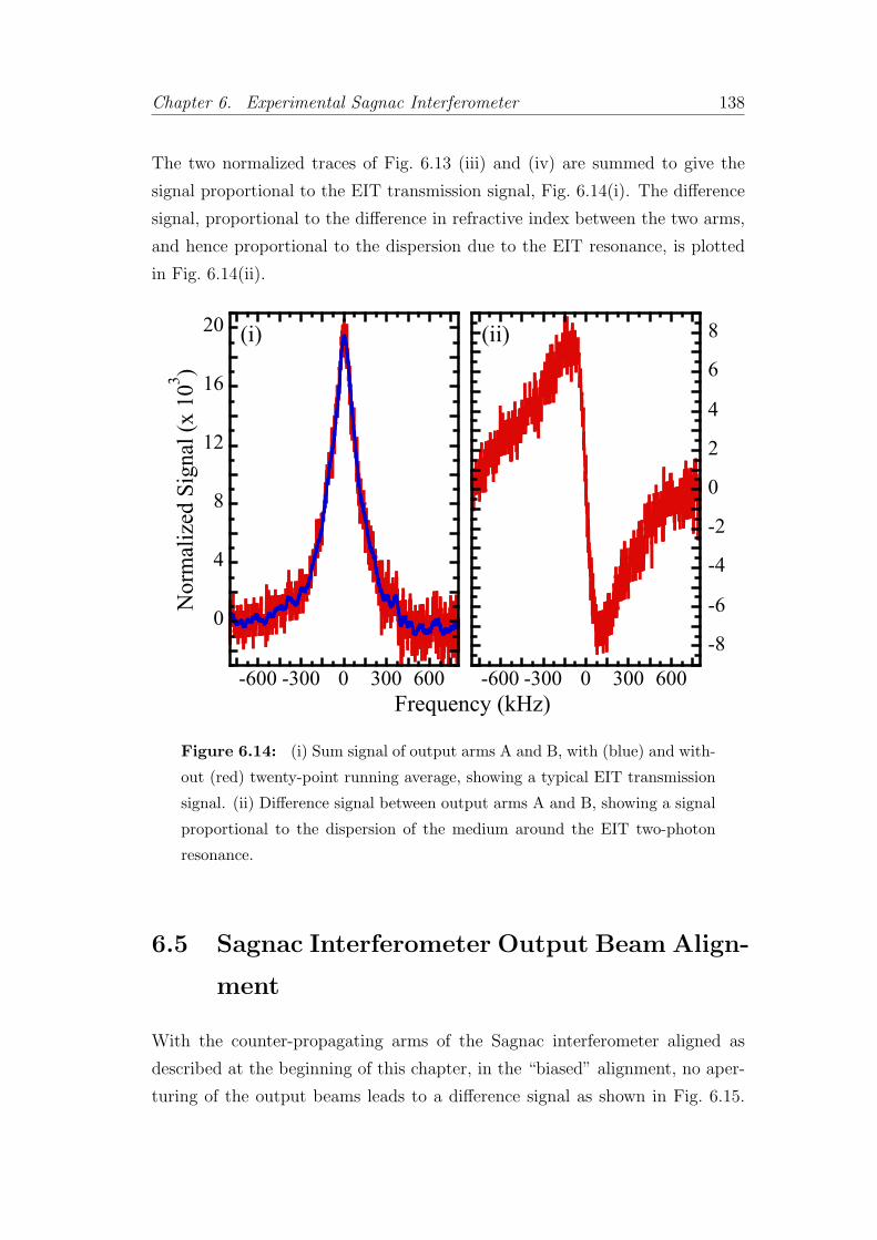
The two normalized traces of Fig. 6.13 (iii) and (iv) are summed to give the

signal proportional to the EIT transmission signal, Fig. 6.14(i). The di!erence

signal, proportional to the di!erence in refractive index between the two arms,

and hence proportional to the dispersion due to the EIT resonance, is plotted

in Fig. 6.14(ii).

0

4

8

12

16

20

-600 -300 0 300 600

No

rmal

ized

Sig

nal

(x

10

3)

-8

-6

-4

-2

0

2

4

6

8

-600 -300 0 300 600

Frequency (kHz)

(i) (ii)

Figure 6.14: (i) Sum signal of output arms A and B, with (blue) and with-

out (red) twenty-point running average, showing a typical EIT transmission

signal. (ii) Difference signal between output arms A and B, showing a signal

proportional to the dispersion of the medium around the EIT two-photon

resonance.

6.5 Sagnac Interferometer Output Beam Align-

ment

With the counter-propagating arms of the Sagnac interferometer aligned as

described at the beginning of this chapter, in the “biased” alignment, no aper-

turing of the output beams leads to a di!erence signal as shown in Fig. 6.15.


Fig. 6.16 shows the di!erence signals for the aperture positions shown in Fig. 6.17,

-8

-4

0

4

8

12

-300 -150 0 150 300

Ph

oto

dio

de

Sig

nal

(m

V)

Frequency (kHz)

Figure 6.15: Difference signal recorded for no slits in the output arm fringe

patterns. The clockwise probe power is 3 µW and the pump power is 10 µW.

As is clearly shown in the figure, the spectrum in the absence of the output

arm apertures is not of the form of a dispersion spectrum.

(i) and (ii) have the aperture positions in each of the two output arms being on

the same side of the beams, while (iii) and (iv) have the apertures on opposite

sides of the output beams.


-8

-4

0

4

8

-300 -150 0 150 300

0

4

8

-300 -150 0 150 300

(i)

(iii) (iv)

(ii)

Frequency (kHz)

Photo

dio

de

Sig

nal

(m

V)

Figure 6.16: (i) Standard aperture position. (ii) Both slits on the opposite

side of beams. (i) and (ii) show that provided both slits are set to the correct

width and that they are both on the same sides of the two beams, a signal

proportional to the dispersion of the medium will be obtained. (iii) Slit A

on standard side of beam, slit B on opposite side of beam. (iv) Slit A on

opposite side of beam, slit B on standard side of beam. (iii) and (iv) show

that if the slits are on opposite sides of the two different beams, the signals

will not be proportional to the dispersion. The clockwise probe and pump

powers are 2 µW and 10 µW.


(i)

(iii) (iv)

(ii)Arm A Arm A Arm BArm B

Figure 6.17: The aperture positions shown in this figure are those used to

record the traces in Fig. 6.16. Each of the four different combinations shown

in this figure corresponds to the same plot in Fig. 6.16.


6.6 EIT Line Width

Details of theoretical line shapes are given in chapter 3. If the signals are

-500 0 500 -500 0 500-2

-1

0

1

-500 0 500

0

4

8

12

16

20

Frequency (kHz)

No

rmal

ized

Sig

nal

(x

10

3)

(i) (ii) (iii)

(vi)(v)(iv)

Figure 6.18: This figure compares three different predicted line shapes to

the measured EIT transmission signals. In (i), (ii) and (iii), the experimental

data is plotted (red), with the theoretical line shape fit (blue). (i) Lorentzian

fit; (ii) arctan fit; and (iii) cusp fit. (iv) Experimental data minus Lorentzian

fit; (v) experimental data minus arctan fit; and (vi) experimental data minus

cusp fit. The clockwise probe power is 3 µW and the pump power is 28 µW.

power broadened, the beam profile a!ects the line shape and width of the reso-

nance, [68]: a step-like beam profile leads to a Lorentzian line shape and a Gaus-


sian beam profile to an arctan line shape. The cusp function gives the expected

line shape for transit-time dominated broadening, [66], and is virtually indistin-

guishable from the arctan fit, [68]. Fig. 6.18(i), (ii) and (iii) all show the twenty-

point moving average transmission EIT feature with weighted least square fits

of the Lorentzian, arctan and cusp functions respectively. Fig. 6.18(iv), (v), and

(vi) show the residual signal — data minus theoretical fit — for Lorentzian, arc-

tan and cusp functions respectively. It can be seen that away from the centre

of the two-photon resonance (detuning greater than ±200 kHz), the residuals

are essentially the same for the three di!erent fits. Only in the central region

(detuning less than ±200 kHz) is there any significant di!erence between any

of the residual traces. The arctan and cusp fits are very similar. Either side

of the centre of the resonance, the amplitude of the experimental line shape is

larger than that of the fit, but on the centre of the resonance (detuning less

than ±50 kHz), the fit value exceeds the data by approximately 10%. The

Lorentzian fit has a higher value than the data either side of the resonance, but

in the region around the centre of the resonance (detuning less than ±30 kHz),

the fit is approximately 5% less than the experimental data.

The reduced χ2 values for each of the three functions suggest that none of

the models truly fit the data. Across the two-photon detuning of #300 kHz to

+300 kHz the reduced χ2 values are 5.59, 9.26, and 5.63, for Lorentzian, arctan,

and cusp fits respectively. Over the wider detuning of ±900 kHz, the reduced χ2

values are 6.29, 7.15, and 5.74. Hence away from resonance the cusp fit gives the

better fit whilst in the region of the resonance the Lorentzian fit is marginally

the best fit. Were any of the functions an accurate fit, then a reduced χ2 value

of between one and two would be expected. In order to quantify the FWHM

and amplitude of the EIT resonances for di!erent pump and probe powers, the

Lorentzian model was used. Rather than fitting the Lorentzian to the sum

signal, the Lorentzian dispersion is fitted to the di!erence signal between the

two arms. The Lorentzian dispersion line shape takes the form of equation 3.80

on page 70,

nR # 1 = #Nd2ba

2ε0!· δpr # δpu

(δpr # δpu)2 + (#a/2)2 .


6.6.1 EIT Line Shape Dependance on Pump and Probe

Power

EIT resonance spectra are recorded for three di!erent regimes of pump and

probe power, Ppu and Ppr respectively.

• Ppr fixed and Ppu varied in the region, 2Ppr ! Ppu ! 20Ppr .

• Ppu fixed and Ppr varied in the region, Ppu/40 ! Ppr ! 0.8Ppu .

• Ppr = Ppu , and both are varied.

Dependence on Pump Power

Variation in amplitude and FWHM of the two-photon EIT resonance, with

increasing pump beam power, is plotted in Fig. 6.19(i) and (ii) respectively.

The amplitude of the features increases with pump power until it starts to

12

17

22

27

32

Am

pli

tude

(mV

)

180

220

260

0 10 20 30 40 50 60 70

FW

HM

(kH

z)

Pump Power (µW)

(i)

(ii)

Figure 6.19: (i) Plot of the amplitude of the EIT features as a function

of pump power. (ii) Plot of the FWHM of a Lorentzian dispersion fit to the

difference signal for a range of pump powers. The probe power is 4 µW.

saturate at around 20 µW, Fig. 6.19(i).


Reducing the intensity of the pump reduces the width of the resonances, as can

be seen in Fig. 6.19(ii). Extrapolating the linear fit of Fig. 6.19(ii), shows that

reducing the pump power to zero will lead to a FWHM of 170 kHz, where the

probe power is 4 µW.

Dependence on Probe Power

0

10

20

30

Am

pli

tud

e (m

V)

120

160

200

0 2 4 6 8

FW

HM

(k

Hz)

Probe Power (µW)

(i)

(ii)

Figure 6.20: (i) Plot of the amplitude of the EIT signal against probe

power. (ii) Plot of the FWHM of a Lorentzian dispersion fit to the difference

signal for a range of pump powers. The pump power is 10 µW.

Fig. 6.20(i) shows that the amplitude of the EIT signal increases linearly with

probe power (with a constant o!set). This is to be expected in the case that

the probe does not e!ect the amplitude of the absorption coe$cient. The linear

increase in the measured amplitude is due to the linear increase in the power of

the incident beam. There is one notable exception, the data point at ! 6.5 µW

falls noticeably below the linear line of best fit. The most likely explanation for

this is that the detuning of the pump beam, δpu, had drifted from the centre of

the Doppler-broadened resonance. This would result in a reduction of the EIT

resonance amplitude, (Fig. 6.9 on page 132).


Fig. 6.20(ii) shows the variation of FWHM of the EIT features with probe power.

As can be seen the width of the resonance increases approximately linearly with

probe power hence this data is not in the regime of a weak probe. In the weak

probe regime the probe power would not e!ect the EIT resonance. This is to

be expected, as with a pump power of 10 µW, the probe powers of & 1 µW

to 8 µW are a significant fraction of the pump power, and as such can not be

described as being in the weak probe regime.

Dependence on Simultaneous Variation of Probe & Pump Power

0

10

20

Am

pli

tude

(mV

)

140

160

180

0 2 4 6 8

FW

HM

(kH

z)

Power (µW)

(i)

(ii)

Figure 6.21: (i) Plots of amplitude of EIT signals against the beam power.

(ii) Plots of the FWHM of the EIT resonances against the beam power.

By definition when the pump power is equal to the probe power, the weak probe

regime cannot apply.

Fig. 6.21(i) shows that the amplitude of the feature increases at a rate greater

than linear. There will be two mechanisms leading to the increase in amplitude.

Increasing probe power will lead to a linear increase in amplitude, as seen in

Fig. 6.20(i) . Secondly increasing pump power will lead to an increase in the


transmission of the medium, Fig. 6.19(i). As the probe and pump power are

equal then both will contribute equally to the “pumping” of the medium.

Fig. 6.21(ii) shows the variation in FWHM with beam power. It is apparent

that the data point corresponding to a beam power of ! 0.5 µW is not plotted.

This is due to the fact that the signal to noise ratio was such that whilst the

amplitude could be fitted to an acceptable degree of precision, the FWHM could

not. The data suggests that the increase in FWHM is at an order greater than

linear.

6.6.2 Comparison of EIT Lineshape to Theory

For the system under investigation, 87Rb 5 2S1/2 F = 1 $ 5 2P3/2 F ′ =

0, 1, 2 , the Doppler-broadened resonances have a significant overlap, Fig. 2.4 on

page 28 . Thus it is not possible to consider the experimental EIT resonances

as being due to a single % system. The resonances are due to three di!er-

ent % systems, with the lower states |F = 1; mF = ±1' and excited states,

|F ′ = 0, 1, 2; mF " = 0' .

The single photon transitions in each of the three % systems have di!erent

transition strengths. Thus for the same beam intensities the Rabi frequencies

di!er by the ratio of the square root of the transition strengths, the ratio of

the dipole matrix elements. The dipole matrix element ratio is 2 :(

5 : 1 , for

F ′ = 0, 1, 2 respectively2, [32]. Across the full range of the Doppler-broadened

resonance, the amplitude of the contribution of each di!erent % system varies

with frequency due to the frequency separation between the excited hyperfine

states and due to the Rabi frequency varying with detuning.

Thus it is not trivial to account for the line widths of the measured EIT reso-

nances using the theoretical models presented in chapter 3 .

Magnetic Broadening

An axial magnetic field of ! 1 G is applied to shift the EIT resonances away

from the beat note. This field will lead to broadening of the EIT resonance as

2On this scale the closed transition, |F = 2; mF = +2' $ |F ! = 3; mF ! = +3' has atransition strength of 2

(3 .


the field is not constant along the length of the vapour cell. From § 4.3.4 on

page 102, the broadening of the resonances can be approximated by ! 3 kHz

G−1.

Hence the contribution, of magnetic broadening, to the width of the EIT reso-

nances presented in this chapter will be ! 3 kHz.

Transit Time

The cusp line shape predicted for transit time broadening only applies in the

regime where the pump and probe power do not contribute to the broadening

of the resonance, § 3.5.4 on page 62. As can clearly be seen from Figs. 6.19,

6.20 and 6.21 , the pump and probe powers do contribute to the width of the

resonances. Hence the expected line shape is not that predicted in § 3.5.4 .

However it will still be instructive to consider the contribution of transit time

broadening to the measured line widths. From equation 3.51 ,

#EIT =

(2 ln 2 v

r.

r being the intensity 1/e beam radius, and v the velocity given by equation 3.52

on page 63 . Thus #EIT = 39.1)2π kHz, at room temperature, 293 K, for 87Rb.

Beam Profile

In order for the line shape to be determined by the pump and probe beam

profiles, the relaxation rate of the atoms, #L, must be much less than the inverse

of the transit time of the atoms through the beam, equation 3.55 .

However the relaxation rate of the atoms is limited by the transit time of the

atoms though the cell. The transit time through the cell is not significantly

greater than the transit time of the atoms through the beams. Hence the

measurements presented in this chapter do not fall into the regime where the

beam profile determines the line shape.

Doppler-Broadened Limit

In the case that a single-photon resonance is Doppler broadened, it follows that

an EIT resonance can be narrowed by the same Doppler-broadening mechanism,


§ 3.5.6 on page 65.

In the presence of Doppler broadening, the FWHM of the EIT resonance, #EIT,

is given by equation 3.68 on page 65,

#2EIT =

γcb"2pu

#a· (1 + x)

!1 +

"

1 +4x

(1 + x)2

#.

x is the dimensionless variable given by equation 3.69 on page 65 ,

x =#a

2γcb·$

"pu

WD

%2

.

The Doppler-broadened width can be taken from table 2.2 on page 37 , hence,

WD = 570) 2π MHz and #a = 6.065) 2π MHz.

The ground state coherence decay rate could be limited by any of the following

three mechanisms:

• collisions of atoms with cell walls;

• collisions of atoms with other atoms;

• and atoms leaving the beam.

As the cell diameter is & 10 times larger than the beam diameter, and the cell

length is 4 times the cell diameter, then the rate at which atoms will leave the

beams will dominate over the rate at which they collide with cell walls.

The mean free path of the atoms, l, is the mean distance they travel between

collisions with other atoms. This is given by,

l =1

σN, (6.2)

N is the total number density, and σ is the cross section for Rb—Rb collisions.

At room temperature (293 K), N = 5.65 ) 1015 m−3, equation 2.101 , and

σ ! 2 ) 10−18 m−2, [107], hence the mean free path, l ! 90 m. As l is & 5000

times larger than the diameter of the the cell, this will not limit γcb.

Thus the dominant mechanism in determining the ground state coherence decay

rate, γcb is transit time of the atoms through the beam. Hence,

γcb ! r

v, (6.3)

where v =

&2kBT

m.


Thus, γcb = 39.6 ) 2π kHz at room temperature, 293 K, and with the beam

diameter 1.89 mm, from § 6.2.1 .

The Rabi frequencies for the three di!erent transitions, "F "=0, "F "=1, and "F "=2

are given by,

"F "=0 =1(3· " , (6.4)

"F "=1 =

&5

12· " , (6.5)

"F "=2 =1(12

· " , (6.6)

where " is the Rabi frequency for the closed transition on the 87Rb D2 line,

given by equation 2.59 on page 19,

" =#a(

2·&

I

ISAT.

In order to make predictions of #EIT the intensity, I, is taken to be the mean

intensity over an area encompassing a fraction Z of the power, P , in the beam,

§ H.2. Therefore the intensity is taken to be, IZ by equation H.16,

IZ =Z P

πr20 ln

'' 11−Z

'' ,

where r0 is the 1/e intensity radius.

With all of the above it is now possible to calculate #EIT for the three di!erent

% systems. Plots of #EIT against pump power up to 100 µW are shown in

Fig. 6.22, where Z is taken to be 0.95.

In the case of the regime shown in Fig. 6.22, where x " 1 , the width of the

EIT resonance can be well approximated by equation 3.73 on page 66,

#EIT = "

&γcb

#a.

As γcb and " can only be approximated then there is scope for a systematic

error in the predictions presented in Fig. 6.22 .

Resultant Line Width

The development of a theoretical model, accurately taking account of all broad-

ening mechanisms and optical pumping, is beyond the scope of this experimental


0 20 40 60 80 1000

100

200

300

EIT

FW

HM

(kH

z)

Beam Power (µW)

Figure 6.22: The solid red line shows the prediction for the Λ system with

upper state |F ′ = 0,mF " = 0', the dashed blue line shows the prediction for

the Λ system with upper state |F ′ = 1,mF " = 0', and the dotted green line

shows the prediction for the Λ system with upper state |F ′ = 2,mF " = 0' .

thesis. In order to make an approximation to the resultant expected line width,

due to the contributions of all of the broadening mechanisms presented so far,

the widths due to each contribution have been summed3. Here the probe beam

is assumed to make the same contribution to the width that a pump beam of

the same power would.

The resultant widths are plotted in Fig. 6.23 alongside the experimental mea-

surements for a constant probe power (of 4 µW) and varying pump, as plotted

in Fig. 6.19 .

The theoretical curves underestimate the extent of the broadening for pump

powers up to & 20 µW. For pump powers in the range of & 20 µW to &80 µW the rate of change of width and the absolute values appear to be in good

agreement with the theoretical values.

A potential explanation for the discrepancy in theoretical and experimental line

widths up to pump powers of & 20 µW would be that the constant contributions

to the line width have been underestimated. In order for this to be the case and

yet still to have agreement at higher pump powers, it would follow that the rate

of increase in width attributable to the pump power has been overestimated.

Further experiments varying the beam diameters would be instructive in re-

3The convolution of two Lorentzian functions of width Γ1 and Γ2 is a Lorentzian functionof width Γ3 = Γ1 + Γ2 .


100

200

300

0 20 40 60 80

EIT

FW

HM

(k

Hz)

Pump Power (µW)

Figure 6.23: The solid red line shows the prediction for the Λ system with

upper state |F ′ = 0,mF " = 0', the dashed blue line shows the prediction for

the Λ system with upper state |F ′ = 1,mF " = 0', and the dotted green line

shows the prediction for the Λ system with upper state |F ′ = 2,mF " = 0' .

The pump broadening is taken to be that shown in Fig. 6.22. The probe,

magnetic and transit time broadening contributions are those described in

the text. The experimentally measured values along with the standard error

are plotted with the black data points.

solving this discrepancy. This would allow for investigation of the transit time

e!ect as well as further investigation of the intensity of the pump and probe

fields.

6.6.3 Dependance on Beam Diameter

Ideally EIT resonances would have been recorded in the Sagnac interferometer

for a range of beam diameters. This would have allowed experimental evaluation

of the e!ect of varying the transit time on the EIT line width.

Preliminary measurements were made of EIT resonances, in transmission only,

where a reduction in line width by a factor of 2.2 was seen for a magnification

of the probe and pump beams of 3.1. These measurements were made keeping

all other variables constant.

Maintaining constant beam power but increasing the diameter does lead to a

reduction in intensity. However, comparison of the reduction in intensity, by a

factor of 9.6 (= 3.12) , with any of the experimental plots of line width against

power (Figs. 6.19 , 6.20 and 6.21) show that this is not su$cient to lead to a


reduction in EIT resonance FWHM of 2.2 . Magnifying the beams by a factor

of 3.1 also has the e!ect of increasing the transit time of the atoms through the

beam by the same factor. Thus transit time broadening would be expected to

be reduced by the factor of 3.1 .

It should be noted that these measurements were made without the benefit of

an optical fibre in the experimental set up and as a result the beam profiles

will have been far from Gaussian, due to the numerous optical elements in the

beam path.

Beam diameter in Sagnac interferometer

Several telescopes, of di!erent magnification, were introduced to the Sagnac

interferometer. The aberrations to the wave fronts of the beams due to the lenses

were such that, the interference patterns at the output of the interferometer were

not well enough defined to allow measurements of the dispersion to be made.

6.6.4 Group Velocity

From equation 3.98 on page 72 the group velocity can be calculated at the

frequency of the two-photon resonance. To do this the FWHM of the two-photon

resonance, the normalized transmission in the absence of the EIT signal, the

normalized signal of the peak of the EIT signal and the length of Rb vapour cell

must be known. In the absence of the EIT signal, the normalized transmitted

signal is 0.9. Taking the data presented in Fig. 6.18, from the Lorentzian fit the

FWHM is 230 kHz. The amplitude of the EIT sum signal is 18.5)10−3 and from

equation 5.62 on page 121, assuming that the clockwise and anticlockwise signals

are the same size in the absence of the EIT feature, it follows that at the centre

of the resonance, the transmission EIT signal is 0.90+2) 18.5) 10−3 = 0.937 .

This gives a group velocity of c/650 .

cha pter 6 exp erim en tal sagna c in terfer o met ereandrei/389/sagnac-interferometer-expt.pdf ·...

Documents