cha pter 2 basic p rop erties of sp lines and b-spl ines · cha pter 2 basic p rop erties of sp...

CHAPTER 2

Basic properties of splines andB-splines

In Chapter 1 we introduced splines through a geometric construction of curves based onrepeated averaging, and it turned out that a natural representation of spline curves wasas linear combinations of B-splines. In this chapter we start with a detailed study of themost basic properties of B-splines, illustrated by examples and figures in Section 2.1, andin Section 2.2 we formally define spline functions and spline curves. In Section 2.3 we givea matrix representation of splines and B-splines, and this representation is the basis forour development of much of the theory in later chapters.

2.1 Some simple consequences of the recurrence relationWe saw in Theorem 1.5 that a degree d spline curve f can be constructed from n controlpoints (ci)n

i=1 and n + d + 1 knots (ti)n+d+1i=1 and written as

f =n!

i=1

ciBi,d,

where {Bi,d}ni=1 are B-splines. In this section we will explore B-splines by considering a

number of examples, and deducing some of their most basic properties. For easy referencewe start by recording the definition of B-splines. Since we will mainly be working withfunctions in this chapter, we use x as the independent variable.Definition 2.1. Let d be a nonnegative integer and let t = (tj), the knot vector or knotsequence, be a nondecreasing sequence of real numbers of length at least d + 2. The jthB-spline of degree d with knots t is defined by

Bj,d,t(x) =x! tj

tj+d ! tjBj,d−1,t(x) +

tj+1+d ! x

tj+1+d ! tj+1Bj+1,d−1,t(x), (2.1)

for all real numbers x, with

Bj,0,t(x) =

"1, if tj " x < tj+1;0, otherwise.

(2.2)

35

36 CHAPTER 2. BASIC PROPERTIES OF SPLINES AND B-SPLINES

1.5 2 2.5 3

0.2

0.4

0.6

0.8

1

(a)1.5 2 2.5 3

0.2

0.4

0.6

0.8

1

(b)

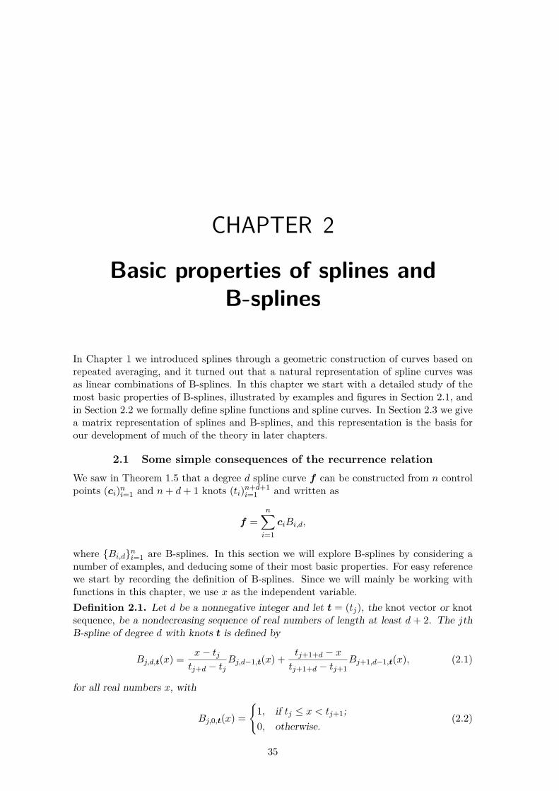
Figure 2.1. A linear B-spline with simple knots (a) and double knots (b).

Here, the convention is assumed that ‘0/0 = 0′. When there is no chance of ambiguity,some of the subscripts will be dropped and the B-spline written as either Bj,d, Bj,t, orsimply Bj .

We say that a knot has multiplicity m if it appears m times in the knot sequence.Knots of multiplicity one, two and three are also called simple, double and triple knots.

Many properties of B-splines can be deduced directly from the definition. One of themost basic properties is that

Bj,d(x) = 0 for all x when tj = tj+d+1

which we made use of in Chapter 1. This is true by definition for d = 0. If it is truefor B-splines of degree d ! 1, the zero convention means that if tj = tj+d+1 then bothBj,d−1(x)/(tj+d ! tj) and Bj+1,d−1(x)/(tj+1+d ! tj+1) on the right in (2.1) are zero, andhence Bj,d(x) is zero. The recurrence relation can therefore be expressed more explicitlyas

Bj,d(x) =

#$$$$%

$$$$&

0, if tj = tj+1+d;s1(x), if tj < tj+d and tj+1 = tj+1+d;s2(x), if tj = tj+d and tj+1 < tj+1+d;s1(x) + s2(x), otherwise;

(2.3)

where

s1(x) =x! tj

tj+d ! tjBj,d−1(x) and s2(x) =

tj+1+d ! x

tj+1+d ! tj+1Bj+1,d−1(x)

for all x.The following example shows that linear B-splines are quite simple.

Example 2.2 (B-splines of degree 1). One application of the recurrence relation gives

Bj,1(x) =x! tj

tj+1 ! tjBj,0(x) +

tj+2 ! xtj+2 ! tj+1

Bj+1,0(x) =(x! tj)/(tj+1 ! tj), if tj " x < tj+1;(tj+2 ! x)/(tj+2 ! tj+1), if tj+1 " x < tj+2;0, otherwise

.

A plot of this hat function is shown in Figure 2.1 (a) in a typical case where tj < tj+1 < tj+2. The figureshows clearly that Bj,1 consists of linear polynomial pieces, with breaks at the knots. In Figure 2.1 (b), thetwo knots tj and tj+1 are identical; then the first linear piece is identically zero since Bj,0 = 0, and Bj,1 isdiscontinuous. This provides an illustration of the smoothness properties of B-splines: a linear B-spline isdiscontinuous at a double knot, but continuous at simple knots.

2.1. SOME SIMPLE CONSEQUENCES OF THE RECURRENCE RELATION 37

2.5 5 7.5 10 12.5 15 17.5

0.2

0.4

0.6

0.8

1

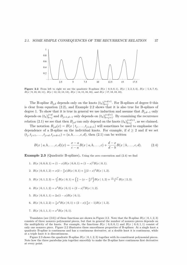
Figure 2.2. From left to right we see the quadratic B-splines B(x | 0, 0, 0, 1), B(x | 2, 2, 3, 4), B(x | 5, 6, 7, 8),B(x | 9, 10, 10, 11), B(x | 12, 12, 13, 13), B(x | 14, 15, 16, 16), and B(x | 17, 18, 18, 18).

The B-spline Bj,d depends only on the knots (tk)j+d+1k=j . For B-splines of degree 0 this

is clear from equation (2.2), and Example 2.2 shows that it is also true for B-splines ofdegree 1. To show that it is true in general we use induction and assume that Bj,d−1 onlydepends on (tk)

j+dk=j and Bj+1,d−1 only depends on (tk)

j+d+1k=j+1. By examining the recurrence

relation (2.1) we see that then Bj,d can only depend on the knots (tk)j+d+1k=j , as we claimed.

The notation Bj,d(x) = B(x | tj , . . . , tj+d+1) will sometimes be used to emphasise thedependence of a B-spline on the individual knots. For example, if d # 2 and if we set(tj , tj+1, . . . , tj+d, tj+d+1) = (a, b, . . . , c, d), then (2.1) can be written

B(x | a, b, . . . , c, d)(x) =x! a

c! aB(x | a, b, . . . , c) +

d! x

d! bB(x | b, . . . , c, d). (2.4)

Example 2.3 (Quadratic B-splines). Using the zero convention and (2.4) we find

1. B(x | 0, 0, 0, 1) = (1! x)B(x | 0, 0, 1) = (1! x)2B(x | 0, 1).

2. B(x | 0, 0, 1, 2) = x(2! 32x)B(x | 0, 1) + 1

2 (2! x)2B(x | 1, 2).

3. B(x | 0, 1, 2, 3) = x2

2 B(x | 0, 1) + 34 ! (x! 3

2 )2 B(x | 1, 2) + (3!x)2

2 B(x | 2, 3).

4. B(x | 0, 1, 1, 2) = x2B(x | 0, 1) + (2! x)2B(x | 1, 2).

5. B(x | 0, 0, 1, 1) = 2x(1! x)B(x | 0, 1).

6. B(x | 0, 1, 2, 2) = 12x2B(x | 0, 1) + (2! x)( 3

2x! 1)B(x | 1, 2).

7. B(x | 0, 1, 1, 1) = x2B(x | 0, 1).

Translates (see (2.6)) of these functions are shown in Figure 2.2. Note that the B-spline B(x | 0, 1, 2, 3)consists of three nonzero polynomial pieces, but that in general the number of nonzero pieces depends onthe multiplicity of the knots. For example, the functions B(x | 0, 0, 0, 1) and B(x | 0, 0, 1, 1) consist ofonly one nonzero piece. Figure 2.2 illustrates these smoothness properties of B-splines: At a single knot aquadratic B-spline is continuous and has a continuous derivative, at a double knot it is continuous, whileat a triple knot it is discontinuous.

Figure 2.3 shows the quadratic B-spline B(x | 0, 1, 2, 3) together with its constituent polynomial pieces.Note how the three parabolas join together smoothly to make the B-spline have continuous first derivativeat every point.


0.5 1 1.5 2 2.5 3

0.2

0.4

0.6

0.8

Figure 2.3. The different polynomial pieces of a quadratic B-spline.

By applying the recurrence relation (2.1) twice we obtain an explicit expression for a generic quadraticB-spline,

Bj,2(x) =x! tj

tj+2 ! tj

x! tj

tj+1 ! tjBj,0(x) +

tj+2 ! xtj+2 ! tj+1

Bj+1,0(x)

+tj+3 ! x

tj+3 ! tj+1

x! tj+1

tj+2 ! tj+1Bj+1,0(x) +

tj+3 ! xtj+3 ! tj+2

Bj+2,0(x)

=(x! tj)

2

(tj+2 ! tj)(tj+1 ! tj)Bj,0(x) +

(tj+3 ! x)2

(tj+3 ! tj+1)(tj+3 ! tj+2)Bj+2,0(x)

+(x! tj)(tj+2 ! x)

(tj+2 ! tj)(tj+2 ! tj+1)+

(tj+3 ! x)(x! tj+1)(tj+3 ! tj+1)(tj+2 ! tj+1)

Bj+1,0(x).

(2.5)

The complexity of this expression gives us a good reason to work with B-splines through other means thanexplicit formulas.

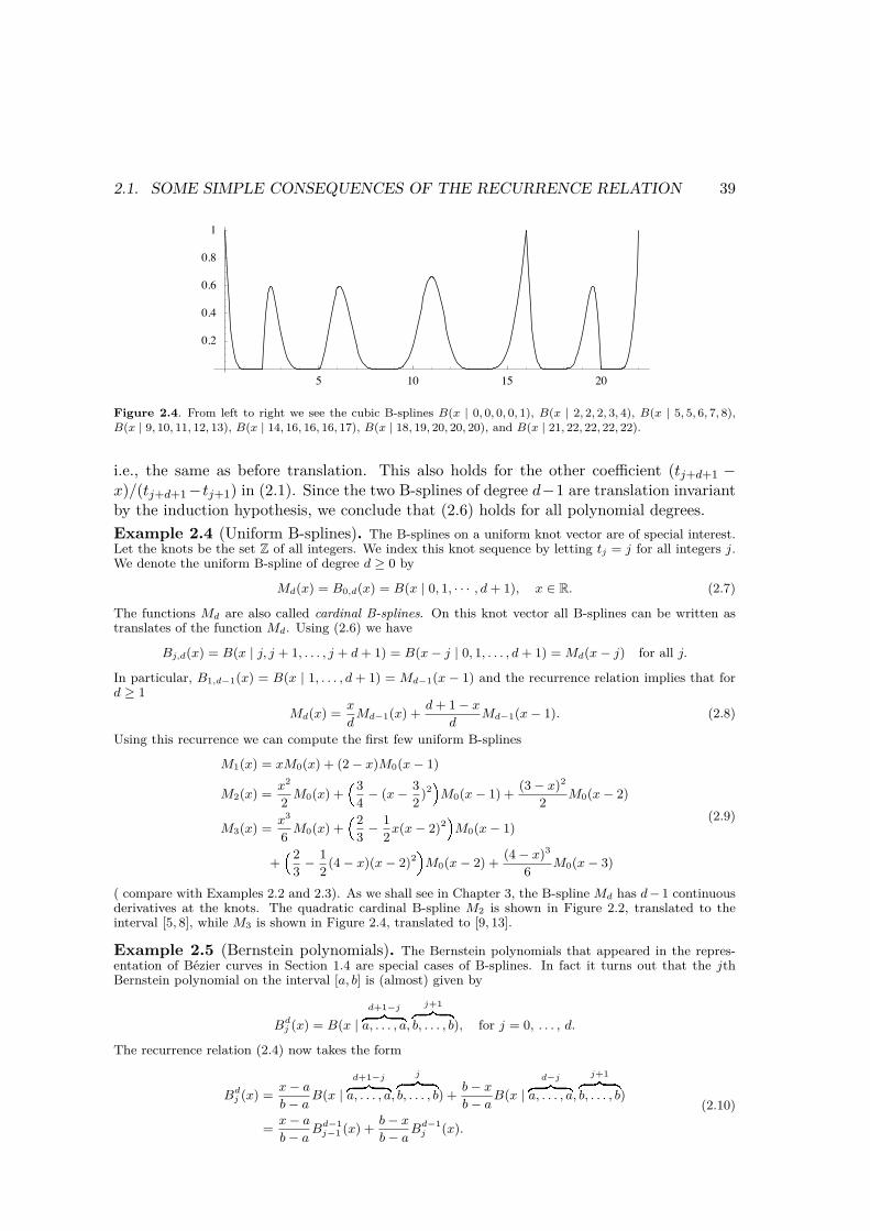
Figure 2.4 shows some cubic B-splines. The middle B-spline, B(x | 9, 10, 11, 12, 13),has simple knots and its second derivative is therefore continuous for all real numbers x,including the knots. In general a cubic B-spline has 3 ! m continuous derivatives at aknot of multiplicity m for m = 1, 2, 3. A cubic B-spline with a knot of multiplicity 4 isdiscontinuous at the knot.

Before considering the next example we show that B-splines possess a property calledtranslation invariance. Mathematically this is expressed by the formula

B(x + y | tj + y, . . . , tj+d+1 + y) = B(x | tj , . . . , tj+d+1) x, y $ R. (2.6)We argue by induction, and start by checking the case d = 0. We have

B(x + y | tj + y, tj+1 + y) =

"1, if tj + y " x + y < tj+1 + y;0, otherwise

=

"1, if tj " x < tj+1;0, otherwise,

so equation (2.6) holds for d = 0. Suppose that the translation invariance holds for B-splines of degree d ! 1. In the recurrence (2.1) for the left-hand-side of (2.6) the firstcoe!cient (x! tj)/(tj+d ! tj) can be written

(x + y)! (tj + y)(tj+d + y)! (tj + y)

=x! tj

tj+d ! tj,

2.1. SOME SIMPLE CONSEQUENCES OF THE RECURRENCE RELATION 39

5 10 15 20

0.2

0.4

0.6

0.8

1

Figure 2.4. From left to right we see the cubic B-splines B(x | 0, 0, 0, 0, 1), B(x | 2, 2, 2, 3, 4), B(x | 5, 5, 6, 7, 8),B(x | 9, 10, 11, 12, 13), B(x | 14, 16, 16, 16, 17), B(x | 18, 19, 20, 20, 20), and B(x | 21, 22, 22, 22, 22).

i.e., the same as before translation. This also holds for the other coe!cient (tj+d+1 !x)/(tj+d+1!tj+1) in (2.1). Since the two B-splines of degree d!1 are translation invariantby the induction hypothesis, we conclude that (2.6) holds for all polynomial degrees.Example 2.4 (Uniform B-splines). The B-splines on a uniform knot vector are of special interest.Let the knots be the set Z of all integers. We index this knot sequence by letting tj = j for all integers j.We denote the uniform B-spline of degree d # 0 by

Md(x) = B0,d(x) = B(x | 0, 1, · · · , d + 1), x $ R. (2.7)

The functions Md are also called cardinal B-splines. On this knot vector all B-splines can be written astranslates of the function Md. Using (2.6) we have

Bj,d(x) = B(x | j, j + 1, . . . , j + d + 1) = B(x! j | 0, 1, . . . , d + 1) = Md(x! j) for all j.

In particular, B1,d!1(x) = B(x | 1, . . . , d + 1) = Md!1(x! 1) and the recurrence relation implies that ford # 1

Md(x) =xd

Md!1(x) +d + 1! x

dMd!1(x! 1). (2.8)

Using this recurrence we can compute the first few uniform B-splines

M1(x) = xM0(x) + (2! x)M0(x! 1)

M2(x) =x2

2M0(x) +

34! (x! 3

2)2 M0(x! 1) +

(3! x)2

2M0(x! 2)

M3(x) =x3

6M0(x) +

23! 1

2x(x! 2)2 M0(x! 1)

+23! 1

2(4! x)(x! 2)2 M0(x! 2) +

(4! x)3

6M0(x! 3)

(2.9)

( compare with Examples 2.2 and 2.3). As we shall see in Chapter 3, the B-spline Md has d!1 continuousderivatives at the knots. The quadratic cardinal B-spline M2 is shown in Figure 2.2, translated to theinterval [5, 8], while M3 is shown in Figure 2.4, translated to [9, 13].

Example 2.5 (Bernstein polynomials). The Bernstein polynomials that appeared in the repres-entation of Bézier curves in Section 1.4 are special cases of B-splines. In fact it turns out that the jthBernstein polynomial on the interval [a, b] is (almost) given by

Bdj (x) = B(x |

d+1!j

a, . . . , a,

j+1

b, . . . , b), for j = 0, . . . , d.

The recurrence relation (2.4) now takes the form

Bdj (x) =

x! ab! a

B(x |d+1!j

a, . . . , a,

j

b, . . . , b) +b! xb! a

B(x |d!j

a, . . . , a,

j+1

b, . . . , b)

=x! ab! a

Bd!1j!1 (x) +

b! xb! a

Bd!1j (x).

(2.10)


This is also valid for j = 0 and j = d if we define Bd!1j = 0 for j < 0 and j # d. Using induction on d one

can show the explicit formula

Bdj (x) =

dj

x! ab! a

j b! xb! a

d!j

B(x | a, b), for j = 0, 1, . . . , d, (2.11)

see exercise 5. These are essentially the Bernstein polynomials for the interval [a, b], except that the factorB(x | a, b) causes Bd

j to be zero outside [a, b]. To represent Bézier curves, it is most common to use theBernstein polynomials on the interval [0, 1] as in Section 1.4, i.e., with a = 0 and b = 1,

Bdj (x) =

dj

xj(1! x)d!jB(x | 0, 1) = bj,d(x)B(x | 0, 1), for j = 0, 1, . . . , d; (2.12)

here bdj is the jth Bernstein polynomial of degree d. For example, the quadratic Bernstein basis polynomials

are given byb0,2(x) = (1! x)2, b1,2(x) = 2x(1! x), b2,2(x) = x2

which agrees with what we found in Chapter 1. These functions can also be recognised as the polynomialpart of the special quadratic B-splines in (1), (5) and (7) in Example 2.3. For Bernstein polynomials on[0, 1] the recurrence relation (2.10) takes the form

bj,d(x) = xbj!1,d!1(x) + (1! x)bj,d!1(x), j = 0, 1, . . . , d. (2.13)

We have now seen a number of examples of B-splines and some characteristic featuresare evident. The following lemma sums up the most basic properties.Lemma 2.6. Let d be a nonnegative polynomial degree and let t = (tj) be a knotsequence. The B-splines on t have the following properties:

1. Local knots. The jth B-spline Bj,d depends only on the knots tj , tj+1, . . . , tj+d+1.

2. Local support.

(a) If x is outside the interval [tj , tj+d+1) then Bj,d(x) = 0. In particular, if tj =tj+d+1 then Bj,d is identically zero.

(b) If x lies in the interval [tµ, tµ+1) then Bj,d(x) = 0 if j < µ! d or j > µ.

3. Positivity. If x $ (tj , tj+d+1) then Bj,d(x) > 0. The closed interval [tj , tj+d+1] iscalled the support of Bj,d.

4. Piecewise polynomial. The B-spline Bj,d can be written

Bj,d(x) =j+d!

k=j

Bkj,d(x)Bk,0(x) (2.14)

where each Bkj,d(x) is a polynomial of degree d.

5. Special values. If z = tj+1 = · · · = tj+d < tj+d+1 then Bj,d(z) = 1 and Bi,d(z) = 0for i %= j.

6. Smoothness. If the number z occurs m times among tj , . . . , tj+d+1 then the deriv-atives of Bj,d of order 0, 1, . . . , d!m are all continuous at z.

Proof. Properties 1–3 follow directly, by induction, from the recurrence relation, seeexercise 3. In Section 1.5 in Chapter 1 we saw that the construction of splines producedpiecewise polynomials, so this explains property 4. Property 5 is proved in exercise 6 andproperty 6 will be proved in Chapter 3.

2.2. LINEAR COMBINATIONS OF B-SPLINES 41

2.2 Linear combinations of B-splinesIn Theorem 1.5 we saw that B-splines play a central role in the representation of splinecurves. The purpose of this section is to define precisely what we mean by spline functionsand spline curves and related concepts like the control polygon.

2.2.1 Spline functionsThe B-spline Bj,d depends on the knots tj , . . . , tj+1+d. This means that if the knot vectoris given by t = (tj)n+d+1

j=1 for some positive integer n, we can form n B-splines {Bj,d}nj=1 of

degree d associated with this knot vector. A linear combination of B-splines, or a splinefunction, is a combination of B-splines on the form

f =n!

j=1

cjBj,d, (2.15)

where c = (cj)nj=1 are n real numbers. We formalise this in a definition.

Definition 2.7 (Spline functions). Let t = (tj)n+d+1j=1 be a nondecreasing sequence of

real numbers, i.e., a knot vector for a total of n B-splines. The linear space of all linearcombinations of these B-splines is the spline space Sd,t defined by

Sd,t = span{B1,d, . . . , Bn,d} =' n!

j=1

cjBj,d | cj $ R for 1 " j " n(

.

An element f =)n

j=1 cjBj,d of Sd,t is called a spline function, or just a spline, of degreed with knots t, and (cj)n

j=1 are called the B-spline coe!cients of f .As we shall see later, B-splines are linearly independent so Sd,t is a linear space of

dimension n.It will often be the case that the exact length of the knot vector is of little interest.

Then we may write a spline as)

j cjBj,d without specifying the upper and lower boundson j.Example 2.8 (A linear spline). Let (xi, yi)

mi=1 be a set of data points with xi < xi+1 for i = 1, 2,

. . . , m! 1. On the knot vector

t = (tj)m+2j=1 = (x1, x1, x2, x3, . . . , xm!1, xm, xm)

we consider the linear (d = 1) spline function

s(x) =m

j=1

yjBj,1(x), for x $ [x1, xm].

From Example 2.2 we see that s satisfies the interpolatory conditions

s(xi) =m

j=1

yjBj,1(xi) = yi, i = 1, . . . , m! 1 (2.16)

since Bi,1(xi) = 1 and all other B-splines are zero at xi. At x = xm all the B-splines are zero according toDefinition 2.1. But the limit of Bm(x) when x tends to xm from the left is 1. Equation (2.16) therefore


2 4 6 8

!1

!0.5

0.5

1

1.5

2

(a)

0.5 1 1.5 2 2.5 3

!1.5

!1

!0.5

0.5

1

(b)

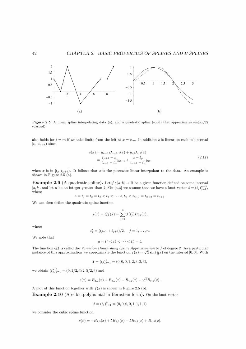
Figure 2.5. A linear spline interpolating data (a), and a quadratic spline (solid) that approximates sin(!x/2)(dashed).

also holds for i = m if we take limits from the left at x = xm. In addition s is linear on each subinterval[tµ, tµ+1) since

s(x) = yµ!1Bµ!1,1(x) + yµBµ,1(x)

=tµ+1 ! xtµ+1 ! tµ

yµ!1 +x! tµ

tµ+1 ! tµyµ.

(2.17)

when x is in [tµ, tµ+1). It follows that s is the piecewise linear interpolant to the data. An example isshown in Figure 2.5 (a).

Example 2.9 (A quadratic spline). Let f : [a, b]% R be a given function defined on some interval[a, b], and let n be an integer greater than 2. On [a, b] we assume that we have a knot vector t = (tj)

n+3j=1 ,

wherea = t1 = t2 = t3 < t4 < · · · < tn < tn+1 = tn+2 = tn+3.

We can then define the quadratic spline function

s(x) = Qf(x) =n

j=1

f(t"j )Bj,2(x),

wheret"j = (tj+1 + tj+2)/2, j = 1, . . . , n.

We note thata = t"1 < t"2 < · · · < t"n = b.

The function Qf is called the Variation Diminishing Spline Approximation to f of degree 2. As a particularinstance of this approximation we approximate the function f(x) =

&2 sin (π

2 x) on the interval [0, 3]. With

t = (tj)8j=1 = (0, 0, 0, 1, 2, 3, 3, 3),

we obtain (t"j )5j=1 = (0, 1/2, 3/2, 5/2, 3) and

s(x) = B2,2(x) + B3,2(x)!B4,2(x)!&

2B5,2(x).

A plot of this function together with f(x) is shown in Figure 2.5 (b).Example 2.10 (A cubic polynomial in Bernstein form). On the knot vector

t = (tj)8j=1 = (0, 0, 0, 0, 1, 1, 1, 1)

we consider the cubic spline function

s(x) = !B1,3(x) + 5B2,3(x)! 5B3,3(x) + B4,3(x).

2.2. LINEAR COMBINATIONS OF B-SPLINES 43

0.5 1 1.5 2 2.5 3

!1

!0.5

0.5

1

(a)

0.2 0.4 0.6 0.8 1

!4

!2

2

4

(b)

Figure 2.6. The quadratic spline from Example 2.9 with its control polygon (a) and the cubic Chebyshev polynomialwith its control polygon (b).

In terms of the cubic Bernstein basis we have

s(x) = !b0,3(x) + 5b1,3(x)! 5b2,3 + b3,3, 0 " x " 1.

This polynomial is shown in Figure 2.6 (b). It is the cubic Chebyshev polynomial with respect to theinterval [0, 1].

Note that the knot vectors in the above examples all have knots of multiplicity d + 1at both ends. If in addition no knot occurs with multiplicity higher than d + 1 (as in theexamples), the knot vector is said to be d + 1-regular.

When we introduced spline curves in Chapter 1, we saw that a curve mimicked theshape of its control polygon in an intuitive way. The control polygon of a spline functionis not quite as simple as for curves since the B-spline coe!cients of a spline function is anumber. What is needed is an abscissa to associate with each coe!cient.Definition 2.11 (Control polygon for spline functions). Let f =

)nj=1 cjBj,d be a spline

in Sd,t. The control points of f are the points with coordinates (t∗j , cj) for j = 1, . . . , n,where

t∗j =tj+1 + · · · + tj+d

d

are the knot averages of t. The control polygon of f is the piecewise linear functionobtained by connecting neighbouring control points by straight lines.

Some spline functions are shown with their control polygons in Figures 2.6–2.7. Itis quite striking how the spline is a smoothed out version of the control polygon. Inparticular we notice that at a knot with multiplicity at least d, the spline and its controlpolygon agree. This happens at the beginning and end of all the splines since we haveused d + 1-regular knot vectors, and also at some points in the interior for the splines inFigure 2.7. We also note that the control polygon is tangent to the spline function at aknot of multiplicity d or d + 1. This close relationship between a spline and its controlpolygon is a geometric instance of one of the many nice properties possessed by splinesrepresented in terms of B-splines.

From our knowledge of B-splines we immediately obtain some basic properties ofsplines.Lemma 2.12. Let t = (tj)n+d+1

j=1 be a knot vector for splines of degree d with n # d + 1,and let f =

)nj=1 cjBj,d be a spline in Sd,t. Then f has the following properties:


0.5 1 1.5 2 2.5 3

0.5

1

1.5

2

(a)1 2 3 4 5

1

2

3

4

5

6

(b)

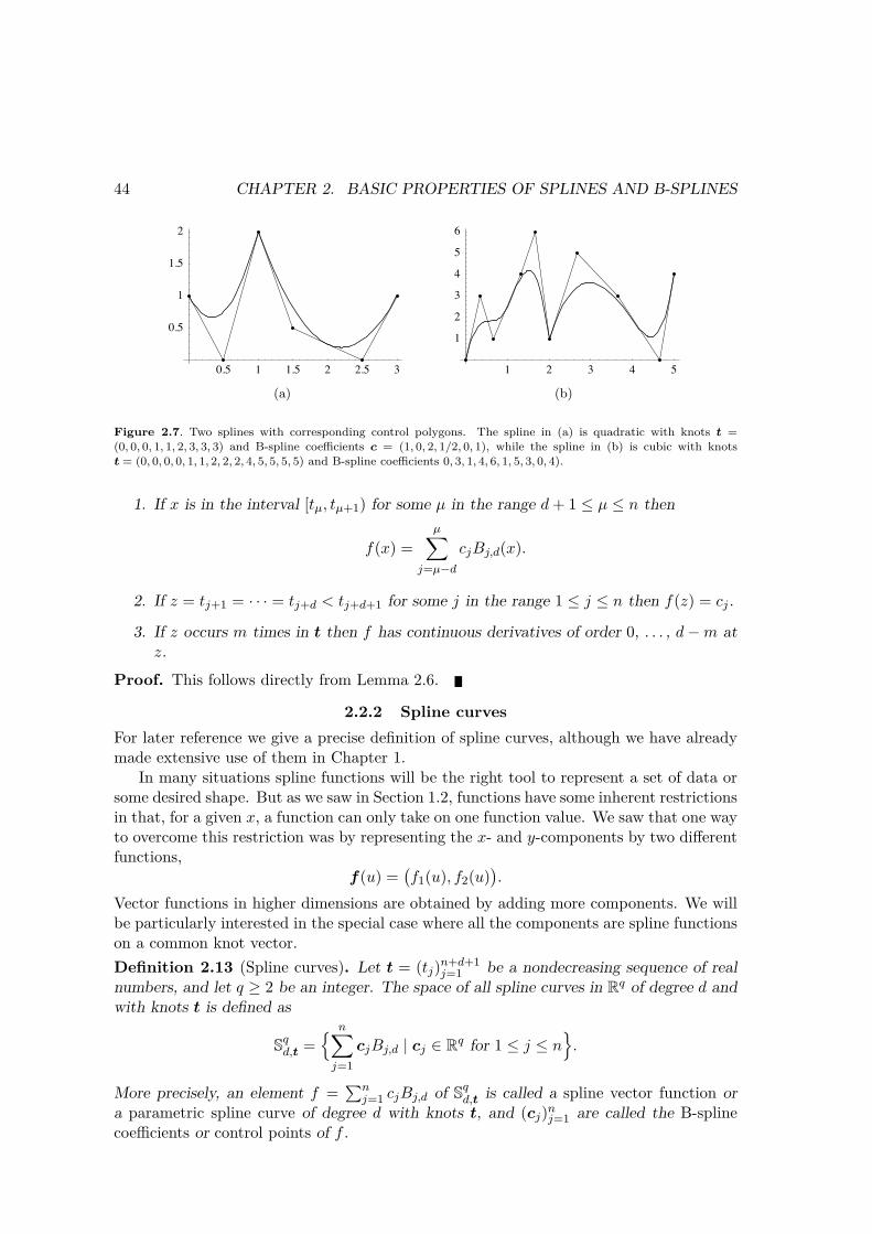
Figure 2.7. Two splines with corresponding control polygons. The spline in (a) is quadratic with knots t =(0, 0, 0, 1, 1, 2, 3, 3, 3) and B-spline coefficients c = (1, 0, 2, 1/2, 0, 1), while the spline in (b) is cubic with knotst = (0, 0, 0, 0, 1, 1, 2, 2, 2, 4, 5, 5, 5, 5) and B-spline coefficients 0, 3, 1, 4, 6, 1, 5, 3, 0, 4).

1. If x is in the interval [tµ, tµ+1) for some µ in the range d + 1 " µ " n then

f(x) =µ!

j=µ−d

cjBj,d(x).

2. If z = tj+1 = · · · = tj+d < tj+d+1 for some j in the range 1 " j " n then f(z) = cj .

3. If z occurs m times in t then f has continuous derivatives of order 0, . . . , d!m atz.

Proof. This follows directly from Lemma 2.6.

2.2.2 Spline curvesFor later reference we give a precise definition of spline curves, although we have alreadymade extensive use of them in Chapter 1.

In many situations spline functions will be the right tool to represent a set of data orsome desired shape. But as we saw in Section 1.2, functions have some inherent restrictionsin that, for a given x, a function can only take on one function value. We saw that one wayto overcome this restriction was by representing the x- and y-components by two di"erentfunctions,

f(u) =*f1(u), f2(u)

+.

Vector functions in higher dimensions are obtained by adding more components. We willbe particularly interested in the special case where all the components are spline functionson a common knot vector.Definition 2.13 (Spline curves). Let t = (tj)n+d+1

j=1 be a nondecreasing sequence of realnumbers, and let q # 2 be an integer. The space of all spline curves in Rq of degree d andwith knots t is defined as

Sqd,t =

' n!

j=1

cjBj,d | cj $ Rq for 1 " j " n(

.

More precisely, an element f =)n

j=1 cjBj,d of Sqd,t is called a spline vector function or

a parametric spline curve of degree d with knots t, and (cj)nj=1 are called the B-spline

coe!cients or control points of f .

2.3. A MATRIX REPRESENTATION OF B-SPLINES 45

We have already defined what we mean by the control polygon of a spline curve, butfor reference we repeat the definition here.Definition 2.14 (Control polygon for spline curves). Let t = (tj)n+d+1

j=1 be a knot vectorfor splines of degree d, and let f =

)nj=1 cjBj,d be a spline curve in Sq

d,t for q # 2. Thecontrol polygon of f is the piecewise linear function obtained by connecting neighbouringcontrol points by straight lines.

Some examples of spline curves with their control polygons can be found in Section 1.5.Spline curves may be thought of as spline functions with B-spline coe!cients that are

vectors. This means that virtually all the algorithms that we develop for spline func-tions can be generalised to spline curves by simply applying the functional version of thealgorithm to each component of the curve in turn.

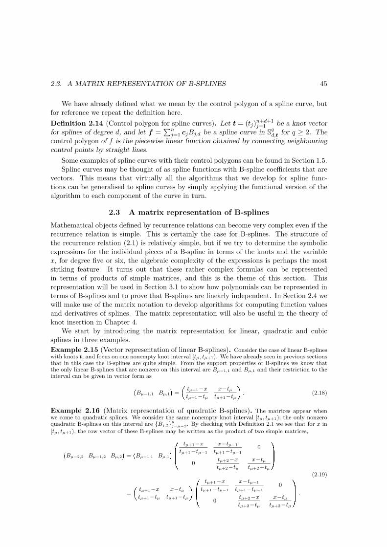
2.3 A matrix representation of B-splinesMathematical objects defined by recurrence relations can become very complex even if therecurrence relation is simple. This is certainly the case for B-splines. The structure ofthe recurrence relation (2.1) is relatively simple, but if we try to determine the symbolicexpressions for the individual pieces of a B-spline in terms of the knots and the variablex, for degree five or six, the algebraic complexity of the expressions is perhaps the moststriking feature. It turns out that these rather complex formulas can be representedin terms of products of simple matrices, and this is the theme of this section. Thisrepresentation will be used in Section 3.1 to show how polynomials can be represented interms of B-splines and to prove that B-splines are linearly independent. In Section 2.4 wewill make use of the matrix notation to develop algorithms for computing function valuesand derivatives of splines. The matrix representation will also be useful in the theory ofknot insertion in Chapter 4.

We start by introducing the matrix representation for linear, quadratic and cubicsplines in three examples.Example 2.15 (Vector representation of linear B-splines). Consider the case of linear B-splineswith knots t, and focus on one nonempty knot interval [tµ, tµ+1). We have already seen in previous sectionsthat in this case the B-splines are quite simple. From the support properties of B-splines we know thatthe only linear B-splines that are nonzero on this interval are Bµ!1,1 and Bµ,1 and their restriction to theinterval can be given in vector form as

Bµ!1,1 Bµ,1 =tµ+1!xtµ+1!tµ

x!tµ

tµ+1!tµ. (2.18)

Example 2.16 (Matrix representation of quadratic B-splines). The matrices appear whenwe come to quadratic splines. We consider the same nonempty knot interval [tµ, tµ+1); the only nonzeroquadratic B-splines on this interval are {Bj,2}µ

j=µ!2. By checking with Definition 2.1 we see that for x in[tµ, tµ+1), the row vector of these B-splines may be written as the product of two simple matrices,

Bµ!2,2 Bµ!1,2 Bµ,2 = Bµ!1,1 Bµ,1

tµ+1!xtµ+1!tµ!1

x!tµ!1

tµ+1!tµ!10

0tµ+2!xtµ+2!tµ

x!tµ

tµ+2!tµ

=tµ+1!xtµ+1!tµ

x!tµ

tµ+1!tµ

tµ+1!xtµ+1!tµ!1

x!tµ!1

tµ+1!tµ!10

0tµ+2!xtµ+2!tµ

x!tµ

tµ+2!tµ

.

(2.19)


If these matrices are multiplied together the result would of course agree with that in Example 2.3.However, the power of the matrix representation lies in the factorisation itself, as we will see in the nextsection. To obtain the value of the B-splines we can multiply the matrices together, but this should bedone numerically, after values have been assigned to the variables. In practise this is only done implicitly,see the algorithms in Section 2.4.Example 2.17 (Matrix representation of cubic B-splines). In the cubic case the only nonzeroB-splines on [tµ, tµ+1) are {Bj,3}µ

j=µ!3. Again it can be checked with Definition 2.1 that for x in thisinterval these B-splines may be written

Bµ!3,3 Bµ!2,3 Bµ!1,3 Bµ,3 = Bµ!2,2 Bµ!1,2 Bµ,2

tµ+1!xtµ+1!tµ!2

x!tµ!2

tµ+1!tµ!20 0

0tµ+2!x

tµ+2!tµ!1

x!tµ!1

tµ+2!tµ!10

0 0tµ+3!xtµ+3!tµ

x!tµ

tµ+3!tµ

=tµ+1!xtµ+1!tµ

x!tµ

tµ+1!tµ

tµ+1!xtµ+1!tµ!1

x!tµ!1

tµ+1!tµ!10

0tµ+2!xtµ+2!tµ

x!tµ

tµ+2!tµ

tµ+1!xtµ+1!tµ!2

x!tµ!2

tµ+1!tµ!20 0

0tµ+2!x

tµ+2!tµ!1

x!tµ!1

tµ+2!tµ!10

0 0tµ+3!xtµ+3!tµ

x!tµ

tµ+3!tµ

.

The matrix notation generalises to B-splines of arbitrary degree in the obvious way.Theorem 2.18. Let t = (tj)n+d+1

j=1 be a knot vector for B-splines of degree d, and let µbe an integer such that tµ < tµ+1 and d + 1 " µ " n. For each positive integer k withk " d define the matrix Rµ

k(x) = Rk(x) by

Rk(x) =

,

---------.

tµ+1!x

tµ+1!tµ+1−k

x!tµ+1−k

tµ+1!tµ+1−k0 · · · 0

0tµ+2!x

tµ+2!tµ+2−k

x!tµ+2−k

tµ+2!tµ+2−k. . . 0

... ... . . . . . . ...0 0 . . .

tµ+k!x

tµ+k!tµ

x!tµtµ+k!tµ

/

0000000001

. (2.20)

Then, for x in the interval [tµ, tµ+1), the d + 1 B-splines {Bj,d}µj=µ−d of degree d that are

nonzero on this interval can be written

BTd =

*Bµ−d,d Bµ−d+1,d . . . Bµ,d

+= R1(x)R2(x) · · ·Rd(x). (2.21)

If f =)

j cjBj,d is a spline in Sd,t, and x is restricted to the interval [tµ, tµ+1), then f(x)is given by

f(x) = R1(x)R2(x) · · ·Rd(x)cd, (2.22)where the vector cd is given by cd = (cµ−d, cµ−d+1, . . . , cµ)T . The matrix Rk is called aB-spline matrix.

2.3. A MATRIX REPRESENTATION OF B-SPLINES 47

For d = 0 the usual convention of interpreting an empty product as 1 is assumed inequations (2.21) and (2.22).

Theorem 2.18 shows how one polynomial piece of splines and B-splines are built up, bymultiplying and adding together (via matrix multiplications) certain linear polynomials.This representation is only an alternative way to write the recurrence relation (2.1), butthe advantage is that all the recursive steps are captured in one equation. This will beconvenient for developing the theory of splines in Section 3.1.2. The factorisation (2.22)will also be helpful for designing algorithms for computing f(x). This is the theme ofSection 2.4.

It should be emphasised that equation (2.21) is a representation of d + 1 polynomials,namely the d + 1 polynomials that make up the d + 1 B-splines on the interval [tµ, tµ+1).This equation can therefore be written

2Bµ

µ−d,d(x) Bµµ−d+1,d(x) . . . Bµ

µ,d(x)3

= Rµ1 (x)Rµ

2 (x) · · ·Rµd(x),

see Lemma 2.6.Likewise, equation (2.22) gives a representation of the polynomial fµ that agrees with

the spline f on the interval [tµ, tµ+1),

fµ(x) = R1(x)R2(x) · · ·Rd(x)cd.

Once µ has been fixed we may let x take values outside the interval [tµ, tµ+1) in both theseequations. In this way the B-spline pieces and the polynomial fµ can be evaluated at anyreal number x. Figure 2.3 was produced in this way.Example 2.19 (Matrix representation of a quadratic spline). In Example 2.9 we consideredthe spline

s(x) = B2,2(x) + B3,2(x)!B4,2(x)!&

2B5,2(x)

on the knot vectort = (tj)

8j=1 = (0, 0, 0, 1, 2, 3, 3, 3).

Let us use the matrix representation to determine this spline explicitly on each of the subintervals [0, 1],[1, 2], and [2, 3]. If x $ [0, 1) then t3 " x < t4 so s(x) is determined by (2.22) with µ = 3 and d = 2. Todetermine the matrices R1 and R2 we use the knots

(tµ!1, tµ, tµ+1, tµ+2) = (0, 0, 1, 2)

and the coefficients(cµ!2, cµ!1, cµ) = (0, 1, 1).

Then equation (2.22) becomes

s(x) = 1! x, x1! x x 0

0 (2! x)/2 x/2

011

= x(2! x)

If x $ [1, 2) then t4 " x < t5 so s(x) is determined by (2.22) with µ = 4 and d = 2. To determine thematrices R1 and R2 in this case we use the knots

(tµ!1, tµ, tµ+1, tµ+2) = (0, 1, 2, 3)

and the coefficients(cµ!2, cµ!1, cµ) = (1, 1,!1).


From this we find

s(x) =12

2! x, x! 12! x x 0

0 3! x x! 1

11!1

= 2x! x2.

For x $ [2, 3) we use µ = 5, and on this interval s(x) is given by

s(x) = 3! x, x! 2(3! x)/2 (x! 1)/2 0

0 3! x x! 2

1!1!&

2= 2! x 6! 2

&2! (2!

&2)x .

2.4 Algorithms for evaluating a splineWe originally introduced spline curves as the result of the geometric construction givenin Algorithm 1.3 in Chapter 1. In this section we will relate this algorithm to the matrixrepresentation of B-splines and develop an alternative algorithm for computing splines.

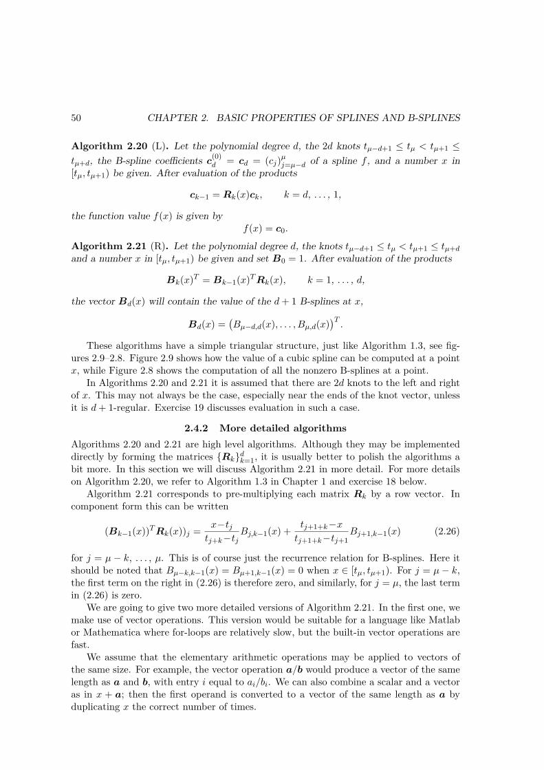
2.4.1 High level descriptionRecall from Theorem 2.18 that a spline f of degree d with knots t and B-spline coe!cientsc can be expressed as

f(x) = R1(x) · · ·Rd(x)cd (2.23)

for any x in the interval [tµ, tµ+1). Here cd = (cµ−d, . . . , cµ) denotes the B-spline coe!cientsthat are active on this interval. To compute f(x) from this representation we have twooptions: We can accumulate the matrix products from left to right or from right to left.

If we start from the right, the computations are

ck−1 = Rkck, for k = d, d! 1, . . . , 1. (2.24)

Upon completion of this we have f(x) = c0 (note that c0 is a vector of dimension 1, i.e.,a scalar). We see that this algorithm amounts to post-multiplying each matrix Rk by avector which in component form becomes

(Rk(x)ck)j =tj+k!x

tj+k!tjcj−1,k +

x!tjtj+k!tj

cj,k (2.25)

for j = µ! k + 1, . . . , µ. This we immediately recognise as Algorithm 1.3.The alternative algorithm accumulates the matrix products in (2.23) from left to right.

This is equivalent to building up the nonzero B-splines at x degree by degree until we haveall the nonzero B-splines of degree d, then multiplying with the corresponding B-splinecoe!cients and summing. Computing the B-splines is accomplished by starting withB0(x)T = 1 and then performing the multiplications

Bk(x)T = Bk−1(x)T Rk(x), k = 1, . . . , d.

The vector Bd(x) will contain the value of the nonzero B-splines of degree d at x,

Bd(x) =*Bµ−d,d(x), . . . , Bµ,d(x)

+T.

We can then multiply with the B-spline coe!cients and add up.

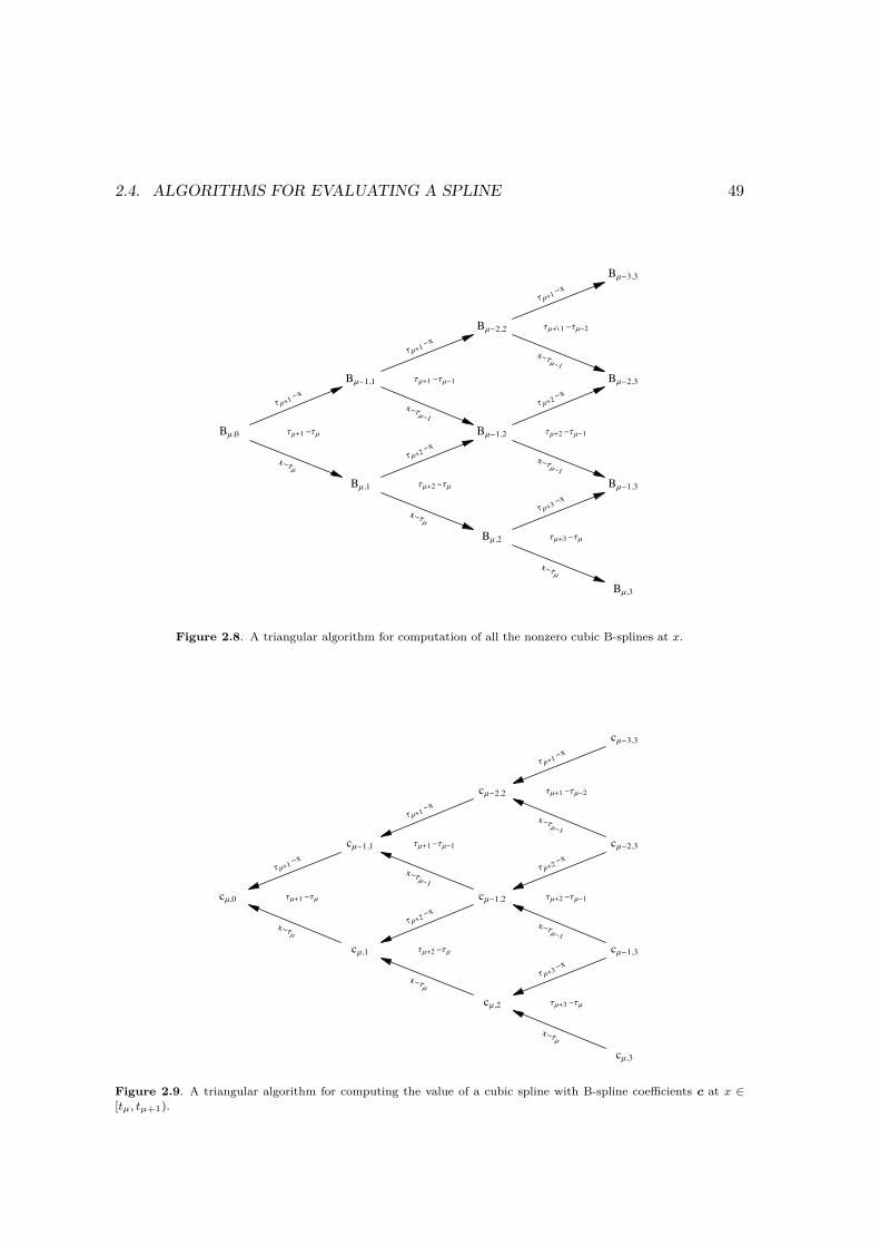
2.4. ALGORITHMS FOR EVALUATING A SPLINE 49

B!,0

"!#1$x

x$"!

"!#1$"!

B!$1,1

"!#1$x

x$"!$1

"!#1$"!$1

B!$2,2

"!#1$x

x$"!$1

"!#\ 1$"!$2

B!,1

"!#2$x

x$"!

"!#2$"!

B!$1,2

"!#2$x

x$"!$1

"!#2$"!$1

B!,2

"!#3$x

x$"!

"!#3$"!

B!$3,3

B!$2,3

B!$1,3

B!,3

Figure 2.8. A triangular algorithm for computation of all the nonzero cubic B-splines at x.

c!,0

"!#1$x

x$"!

"!#1$"!

c!$1,1

"!#1$x

x$"!$1

"!#1$"!$1

c!$2,2

"!#1$x

x$"!$1

"!#1$"!$2

c!,1

"!#2$x

x$"!

"!#2$"!

c!$1,2

"!#2$x

x$"!$1

"!#2$"!$1

c!,2

"!#3$x

x$"!

"!#3$"!

c!$3,3

c!$2,3

c!$1,3

c!,3

Figure 2.9. A triangular algorithm for computing the value of a cubic spline with B-spline coefficients c at x ∈[tµ, tµ+1).


Algorithm 2.20 (L). Let the polynomial degree d, the 2d knots tµ−d+1 " tµ < tµ+1 "tµ+d, the B-spline coefficients c(0)

d = cd = (cj)µj=µ−d of a spline f , and a number x in

[tµ, tµ+1) be given. After evaluation of the products

ck−1 = Rk(x)ck, k = d, . . . , 1,

the function value f(x) is given byf(x) = c0.

Algorithm 2.21 (R). Let the polynomial degree d, the knots tµ−d+1 " tµ < tµ+1 " tµ+d

and a number x in [tµ, tµ+1) be given and set B0 = 1. After evaluation of the products

Bk(x)T = Bk−1(x)T Rk(x), k = 1, . . . , d,

the vector Bd(x) will contain the value of the d + 1 B-splines at x,

Bd(x) =*Bµ−d,d(x), . . . , Bµ,d(x)

+T.

These algorithms have a simple triangular structure, just like Algorithm 1.3, see fig-ures 2.9–2.8. Figure 2.9 shows how the value of a cubic spline can be computed at a pointx, while Figure 2.8 shows the computation of all the nonzero B-splines at a point.

In Algorithms 2.20 and 2.21 it is assumed that there are 2d knots to the left and rightof x. This may not always be the case, especially near the ends of the knot vector, unlessit is d + 1-regular. Exercise 19 discusses evaluation in such a case.

2.4.2 More detailed algorithmsAlgorithms 2.20 and 2.21 are high level algorithms. Although they may be implementeddirectly by forming the matrices {Rk}d

k=1, it is usually better to polish the algorithms abit more. In this section we will discuss Algorithm 2.21 in more detail. For more detailson Algorithm 2.20, we refer to Algorithm 1.3 in Chapter 1 and exercise 18 below.

Algorithm 2.21 corresponds to pre-multiplying each matrix Rk by a row vector. Incomponent form this can be written

(Bk−1(x))T Rk(x))j =x!tj

tj+k!tjBj,k−1(x) +

tj+1+k!x

tj+1+k!tj+1Bj+1,k−1(x) (2.26)

for j = µ ! k, . . . , µ. This is of course just the recurrence relation for B-splines. Here itshould be noted that Bµ−k,k−1(x) = Bµ+1,k−1(x) = 0 when x $ [tµ, tµ+1). For j = µ! k,the first term on the right in (2.26) is therefore zero, and similarly, for j = µ, the last termin (2.26) is zero.

We are going to give two more detailed versions of Algorithm 2.21. In the first one, wemake use of vector operations. This version would be suitable for a language like Matlabor Mathematica where for-loops are relatively slow, but the built-in vector operations arefast.

We assume that the elementary arithmetic operations may be applied to vectors ofthe same size. For example, the vector operation a/b would produce a vector of the samelength as a and b, with entry i equal to ai/bi. We can also combine a scalar and a vectoras in x + a; then the first operand is converted to a vector of the same length as a byduplicating x the correct number of times.


We will need two more vector operations which we denote a+l and a+f . The firstdenotes the vector obtained by appending a zero to the end of a, while a+f denotes theresult of prepending a zero element at the beginning of a. In Matlab syntax this wouldbe written as a+l = [a, 0] and a+f = [0,a]. We leave it to the reader to verify thatAlgorithm 2.21 can then be written in the following more explicit form. A vector versionof Algorithm 2.20 can be found in exercise 18.Algorithm 2.22 (R—vector version). Let the polynomial degree d, the knots tµ−d+1 "tµ < tµ+1 " tµ+d and a number x in [tµ, tµ+1) be given. After evaluation of

1. b = 1;2. For r = 1, 2, . . . , d

1. t1 = (tµ−r+1, . . . , tµ);2. t2 = (tµ+1, . . . , tµ+r);3. ! = (x! t1)/(t2! t1);4. b =

*(1! !) & b

++l

+*! & b

++f

;

the vector b will contain the value of the d + 1 B-splines at x,

b =*Bµ−d,d(x), . . . , Bµ,d(x)

+T.

When programming in a traditional procedural programming language, the vectoroperations will usually have to be replaced by for-loops. This can be accomplished asfollows.Algorithm 2.23 (R—scalar version). Let the polynomial degree d, the knots tµ−d+1 "tµ < tµ+1 " tµ+d and a number x in [tµ, tµ+1) be given. After evaluation of

1. bd+1 = 1; bi = 0, i = 1, . . . , d;2. For r = 1, 2, . . . , d

1. k = µ! r + 1;2. !2 = (tk+r ! x)/(tk+r ! tk);3. bd−r = !2 bd−r+1;4. For i = d! r + 1, d! r + 2, . . . , d! 1

1. k = k + 1;2. !1 = !2;3. !2 = (tk+r ! x)/(tk+r ! tk);4. bi = (1! !1) bi + !2 bi+1;

5. bd = (1! !2) bd

the vector b will contain the value of the d + 1 B-splines at x,

b =*Bµ−d,d(x), . . . , Bµ,d(x)

+T.


Exercises for Chapter 22.1 Show that

B(x | 0, 3, 4, 6) =112

x2B(x | 0, 3) +112

(!7x2 + 48x! 72)B(x | 3, 4)

+16(6! x)2B(x | 4, 6).

2.2 Find the individual polynomial pieces of the following cubic B-splines and discusssmoothness properties at knots

a) B(x | 0, 0, 0, 0, 1) and B(x | 0, 1, 1, 1, 1)b) B(x | 0, 1, 1, 1, 2)

2.3 Show that the B-spline Bj,d satisfies properties 1–3 of Lemma 2.6.

2.4 Show that Bj,d is a piecewise polynomial by establishing equation 2.14. Use inductionon the degree d.

2.5 In this exercise we are going to establish some properties of the Bernstein polyno-mials.

a) Prove the di"erentiation formulaDbj,d(x) = d(bj−1,d−1(x)!Bj,d−1(x)).

b) Show that the Bernstein basis function bj,d(x) has a maximum at x = j/d, andthat this is the only maximum.

c) Show that 4 1

0Bj,d(x)dx = 1/(d + 1).

2.6 a) When a B-spline is evaluated at one of its knots can be simplified according tothe formula

B(ti | tj , . . . , tj+1+d) = B(ti | tj , . . . , ti−1, ti+1, . . . , tj+1+d) (2.27)which is valid for i = j, j + 1, . . . , j + 1 + d. Prove this by induction on thedegree d.

b) Use the formula in (2.27) to compute the following values of a quadratic B-splineat the interior knots:

Bj,2(tj+1) =tj+1 ! tjtj+2 ! tj

, Bj,2(tj+2) =tj+3 ! tj+2

tj+3 ! tj+1. (2.28)

c) Prove property (5) of Lemma 2.6.

2.7 Prove the following formula using (2.4) and (2.11)

B(x | a,

d5 67 8b, . . . , b, c) =

(x! a)d

(b! a)dB(x | a, b) +

(c! x)d

(c! b)dB(x | b, c).

Show that this function is continuous at all real numbers.


2.8 Prove the following formulas by induction on d.

B(x |d5 67 8

a, . . . , a, b, c) =x! a

b! a

d−1!

i=0

(c! x)i(b! x)d−1−i

(c! a)i(b! a)d−1−iB(x | a, b)

+(c! x)d

(c! a)d−1(c! b)B(x | b, c),

B(x | a, b,d5 67 8

c, . . . , c) =(x! a)d

(c! a)d−1(b! a)B(x | a, b)

+c! x

c! b

d−1!

i=0

(x! a)i(x! b)d−1−i

(c! a)i(c! b)d−iB(x | b, c).

2.9 When the knots are simple we can give explicit formulas for the B-splines.

a) Show by induction that if tj < · · · < tj+1+d then

Bj,d(x) = (tj+1+d ! tj)j+1+d!

i=j

(x! ti)d+9j+1+d

k=jk %=i

(tk ! ti)

where

(x! ti)d+ =

"(x! ti)d, if x # ti;0, otherwise.

b) Show that Bj,d can also be written

Bj,d(x) = (tj+1+d ! tj)j+1+d!

i=j

(ti ! x)d+9j+1+d

k=jk %=i

(ti ! tk)

but now the (·)+-function must be defined by

(ti ! x)d+ =

"(ti ! x)d, if ti > x;0, otherwise.

2.10 Write down the matrix R3(x) for µ = 4 in the case of uniform splines (tj = j for allj). Do the same for the Bernstein basis (t = (0, 0, 0, 0, 1, 1, 1, 1)).

2.11 Given a knot vector t = (tj)n+d+1j=1 and a real number x with x $ [t1, tn+d+1), write

a procedure for determining the index µ such that tµ " x < tµ+1. A call to thisroutine is always needed before Algorithms 2.20 and 2.21 are run. By letting µ bean input parameter as well as an output parameter you can minimise the searchingfor example during plotting when the routine is called with many values of x in thesame knot interval.

2.12 Implement Algorithm 2.21 in your favourite programming language.


2.13 Implement Algorithm 2.20 in your favourite programming language.

2.14 Count the number of operations (additions, multiplications, divisions) involved inAlgorithm 2.20.

2.15 Count the number of operations (additions, multiplications, divisions) involved inAlgorithm 2.21.

2.16 Write a program that plots the cubic B-spline B(x | 0, 1, 3, 5, 6) and its polynomialpieces. Present the results as in Figure 2.3.

2.17 a) What is computed by Algorithm 2.20 if x does not belong to the interval[tµ, tµ+1)?

b) Repeat (b) for Algorithm 2.21.

2.18 Algorithm 2.22 gives a vector version of Algorithm 2.21 for computing the nonzero B-splines at a point x. Below is a similar vector version of Algorithm 2.20 for computingthe value of a spline at x. Verify that the algorithm is correct and compare it withAlgorithm 2.22.Let f =

)i ciBi,d,t be a spline in Sd,t, and let x be a real number in the interval

[tµ, tµ+1). Then f(x) can be computed as follows:

1. c = (cµ−k+1, . . . , cµ);2. For r = k ! 1, k ! 2, . . . , 1

1. t1 = (tµ−r+1, . . . , tµ);2. t2 = (tµ+1, . . . , tµ+r);3. ! = (x! t1)/(t2! t1);4. c = (1! !) & c−l + ! & c−f ;

After these statements c will be a vector of length 1 that contains the number f(x).Here the notation c−l and c−f denote the vectors obtained by dropping the last,respectively the first, entry from c.

2.19 Suppose that d = 3 and that the knot vector is given by

t̂ = (tj)5j=1 = (0, 1, 2, 3, 4).

With this knot vector we can only associate one cubic B-spline, namely B1,3. There-fore, if we are to compute B1,3(x) for some x in (0, 4), none of the algorithms of thissection apply. Define the augmented knot vector t by

t = (!1,!1,!1,!1, 0, 1, 2, 3, 4, 5, 5, 5, 5).

Explain how this knot vector can be exploited to compute the B-spline B1,3(x) byAlgorithms 2.20 or 2.21.

cha pter 2 basic p rop erties of sp lines and b-spl ines · cha pter 2 basic p rop erties of sp...

Documents