ch.5. balance principles - upc universitat...
TRANSCRIPT

CH.5. BALANCE PRINCIPLES Continuum Mechanics Course (MMC)

Overview
Balance Principles
Convective Flux or Flux by Mass Transport
Local and Material Derivative of a Volume Integral
Conservation of Mass Spatial Form
Material Form
Reynolds Transport Theorem Reynolds Lemma
General Balance Equation
Linear Momentum Balance Global Form
Local Form
2
Lecture 1
Lecture 2 Lecture 3
Lecture 4
Lecture 7
Lecture 5
Lecture 6
Lecture 8
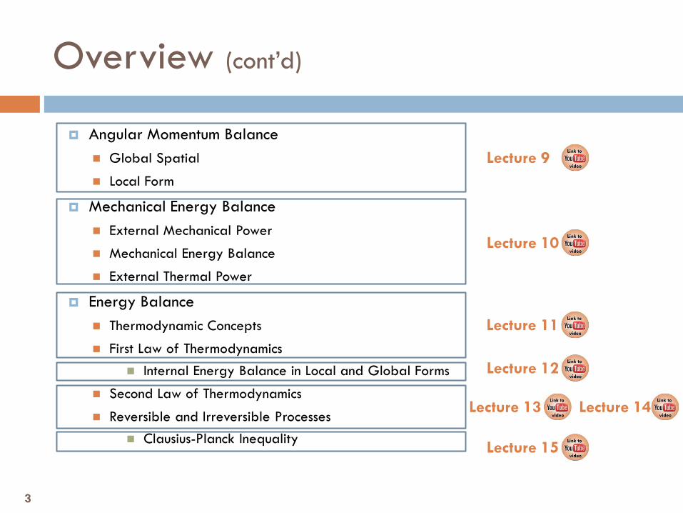
Overview (cont’d)
Angular Momentum Balance Global Spatial
Local Form
Mechanical Energy Balance External Mechanical Power
Mechanical Energy Balance
External Thermal Power
Energy Balance Thermodynamic Concepts
First Law of Thermodynamics Internal Energy Balance in Local and Global Forms
Second Law of Thermodynamics
Reversible and Irreversible Processes Clausius-Planck Inequality
3
Lecture 12
Lecture 13 Lecture 14
Lecture 15
Lecture 9
Lecture 11
Lecture 10
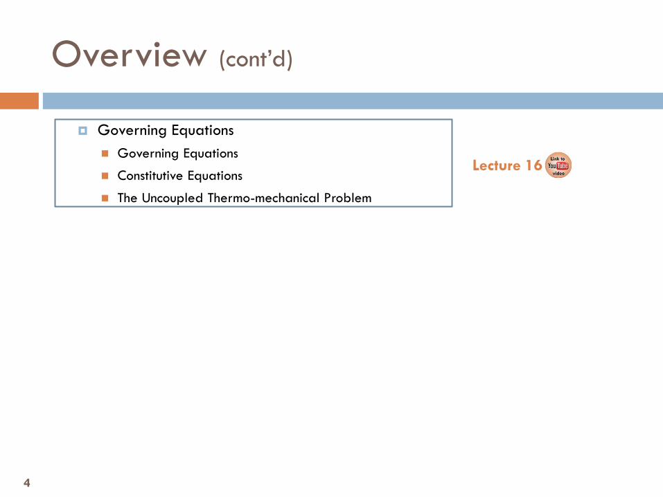
Overview (cont’d)
Governing Equations Governing Equations
Constitutive Equations
The Uncoupled Thermo-mechanical Problem
4
Lecture 16

5
Ch.5. Balance Principles
5.1. Balance Principles

The following principles govern the way stress and deformation vary in the neighborhood of a point with time.
The conservation/balance principles: Conservation of mass Linear momentum balance principle Angular momentum balance principle Energy balance principle or first thermodynamic balance principle
The restriction principle: Second thermodynamic law
The mathematical expressions of these principles will be given in, Global (or integral) form Local (or strong) form
Balance Principles
REMARK These principles are always valid, regardless of the type of material and the range of displacements or deformations.
6
7
Ch.5. Balance Principles
5.2. Convective Flux

The term convection is associated to mass transport, i.e., particle movement. Properties associated to mass will be transported with the mass when
there is mass transport (particles motion)
Convective flux of an arbitrary property through a control
surface :
Convection
SS
Φ =Aamountof crossing
unitof time
convective transport
AS
8

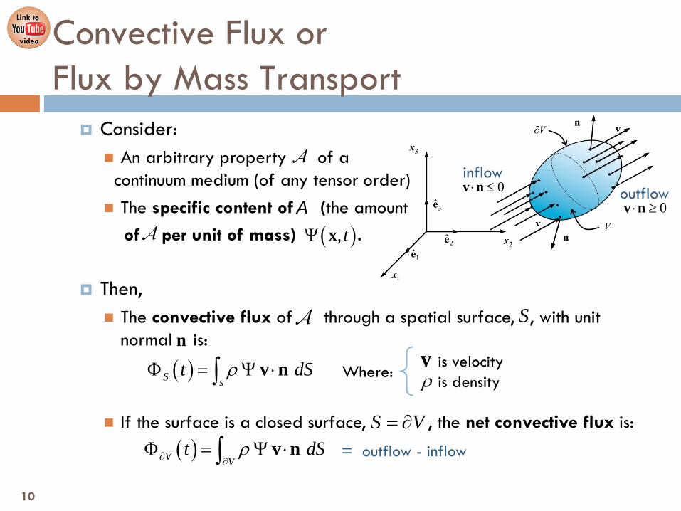
Consider: An arbitrary property of a continuum medium (of any tensor order)
The description of the amount of the property per unit of mass, (specific content of the property ) .
The volume of particles crossing a differential surface during the interval is
Then, The amount of the property crossing the differential surface per unit of
time is:
Convective Flux or Flux by Mass Transport
( ), tΨ x
A
dV dS dh dt dSdm dV dSdtρ ρ
= ⋅ = ⋅= = ⋅
v nv n
Sdmd dS
dtρΨ
Φ = = Ψ ⋅v n
dVdS
[ ],t t dt+
A
9
inflow outflow 0⋅ ≤v n
0⋅ ≥v n
Consider: An arbitrary property of a continuum medium (of any tensor order) The specific content of (the amount of per unit of mass) .
Then, The convective flux of through a spatial surface, , with unit
normal is:
If the surface is a closed surface, , the net convective flux is:
Convective Flux or Flux by Mass Transport
A
( ), tΨ x
A
Sn
( )S st dSρΦ = Ψ ⋅∫ v n
( )V Vt dSρ∂ ∂
Φ = Ψ ⋅∫ v nS V= ∂
= outflow - inflow
Where: is velocity is density ρ
v
A
10
A
Convective Flux
11
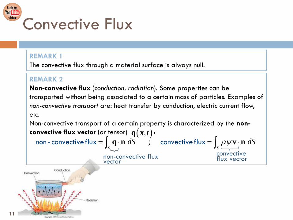
REMARK 1 The convective flux through a material surface is always null.
REMARK 2 Non-convective flux (conduction, radiation). Some properties can be transported without being associated to a certain mass of particles. Examples of non-convective transport are: heat transfer by conduction, electric current flow, etc. Non-convective transport of a certain property is characterized by the non-convective flux vector (or tensor) :
( ), tq x;
s sdS dSρψ= ⋅ = ⋅∫ ∫q n v nconvectiveflnon - convectiveflu ux x
convective flux vector non-convective flux
vector
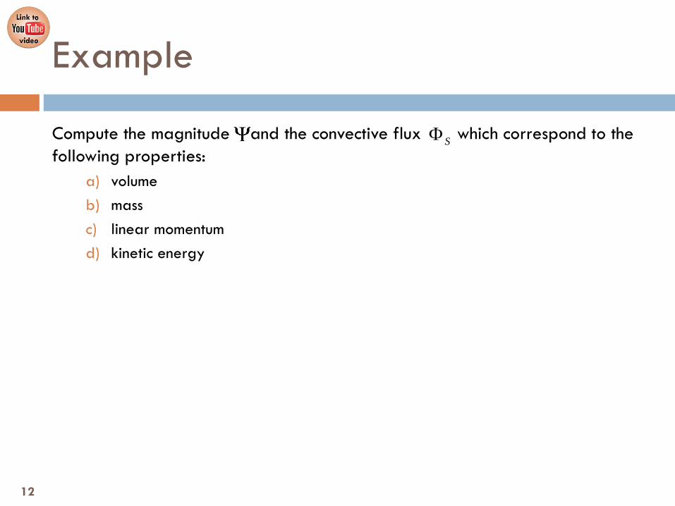
Example
Compute the magnitude and the convective flux which correspond to the following properties:
a) volume b) mass c) linear momentum d) kinetic energy
SΦ
12

Example - Solution
a) If the arbitrary property is the volume of the particles:
The magnitude “property content per unit of mass” is volume per unit of
mass, i.e., the inverse of density:
The convective flux of the volume of the particles through the surface is:
V≡A
1VM ρ
Ψ = =
1S s s
dS dSρρ
Φ = ⋅ = ⋅∫ ∫v n v n
SV
VOLUME FLUX
( )S st dSρΦ = Ψ ⋅∫ v n
13
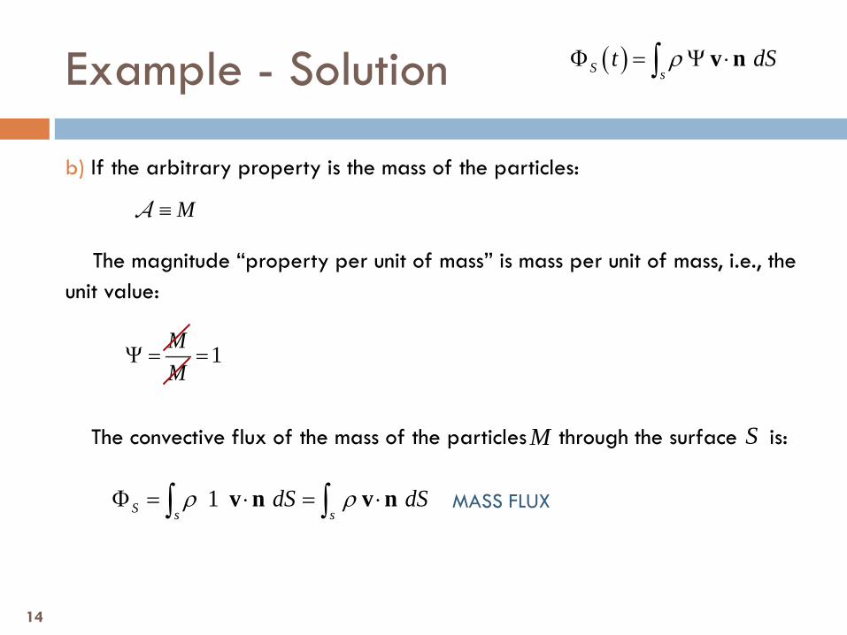
Example - Solution
b) If the arbitrary property is the mass of the particles:
The magnitude “property per unit of mass” is mass per unit of mass, i.e., the unit value:
The convective flux of the mass of the particles through the surface is:
M≡A
1MM
Ψ = =
1S s sdS dSρ ρΦ = ⋅ = ⋅∫ ∫v n v n
SM
MASS FLUX
( )S st dSρΦ = Ψ ⋅∫ v n
14

Example - Solution
c) If the arbitrary property is the linear momentum of the particles:
The magnitude “property per unit of mass” is mass times velocity per unit of mass, i.e., velocity:
The convective flux of the linear momentum of the particles through the surface is:
M≡ vA
MM
= =v vΨ
( )S sdSρ= ⋅∫ v v nΦ
SM v
MOMENTUM FLUX
( )S st dSρΦ = Ψ ⋅∫ v n
15
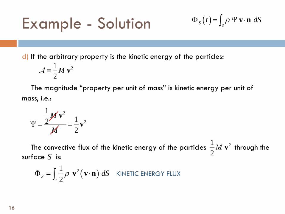
Example - Solution
d) If the arbitrary property is the kinetic energy of the particles:
The magnitude “property per unit of mass” is kinetic energy per unit of mass, i.e.:
The convective flux of the kinetic energy of the particles through the surface is:
212
M≡ vA
2
2
1122
M
MΨ = =
vv
( )212S s
dSρΦ = ⋅∫ v v n
S21
2M v
KINETIC ENERGY FLUX
( )S st dSρΦ = Ψ ⋅∫ v n
16
17
Ch.5. Balance Principles
5.3. Local and Material Derivative of a Volume Integral

Consider: An arbitrary property of a continuum medium (of any tensor order)
The description of the amount of the property per unit of volume
(density of the property ),
The total amount of the property in an arbitrary volume, , is: The time derivative of this volume integral is:
Derivative of a Volume Integral
A
( ), tµ xREMARK and are related through .
Ψ
V
( ) ( ), V
Q t t dVµ= ∫ x
( ) ( ) ( )0
limt
Q t t Q tQ t
t∆ →
+ ∆ −′ =
∆
A
18
( )Q t
( )Q t t+ ∆
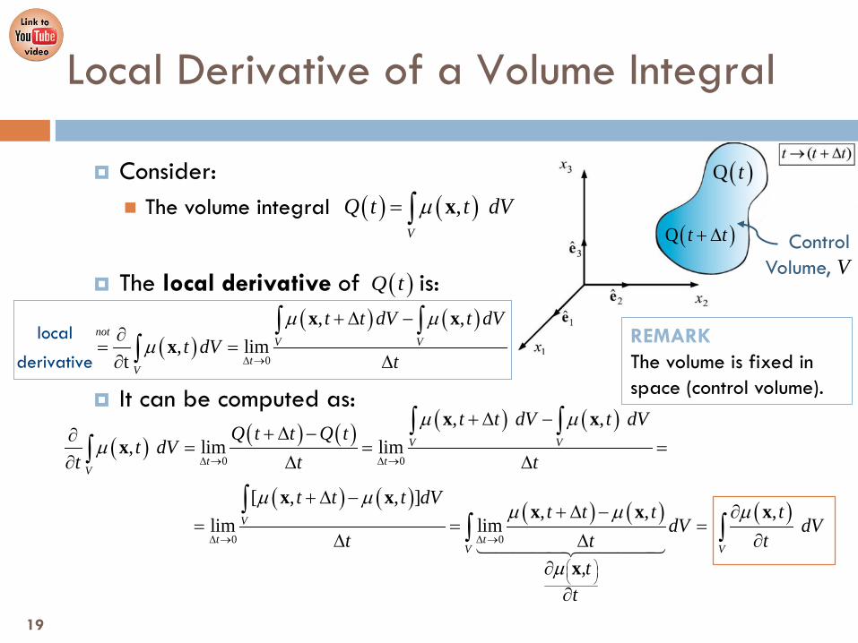
( ) ( ) ( ) ( ) ( )
( ) ( ) ( ) ( ) ( )
0 0
0 0
,
, , , lim lim
[ , , ], , ,
lim lim
V V
t tV
V
t tV V
tt
t t dV t dVQ t t Q t
t dVt t t
t t t dVt t t t
dV dVt t t
µ
µ µµ
µ µµ µ µ
∆ → ∆ →
∆ → ∆ →
∂∂
+ ∆ −+ ∆ −∂
= = =∂ ∆ ∆
+ ∆ −+ ∆ − ∂
= = =∆ ∆ ∂
∫ ∫∫
∫∫ ∫
x
x xx
x xx x x
( )Q t
( )Q t t+ ∆ Control Volume, V
Consider: The volume integral
The local derivative of is:
It can be computed as:
Local Derivative of a Volume Integral
REMARK The volume is fixed in space (control volume).
( ) ( ), V
Q t t dVµ= ∫ x
( )( ) ( )
0
, ,, lim
t
notV V
tV
t t dV t dVt dV
t
µ µµ
∆ →
+ ∆ −∂
= =∂ ∆
∫ ∫∫
x xx
local
derivative
( )Q t
19
( )Q t ( )Q t t+ ∆
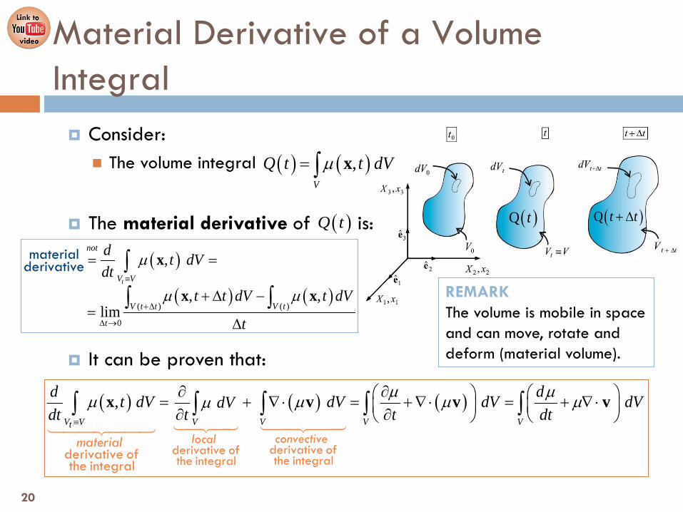
Consider: The volume integral
The material derivative of is:
It can be proven that:
Material Derivative of a Volume Integral
REMARK The volume is mobile in space and can move, rotate and deform (material volume).
( ) ( ),V
Q t t dVµ= ∫ x
( )
( ) ( )( ) ( )
0
,
, ,lim
x
x xt
not
V V
V t t V t
t
d t dVdt
t t dV t dV
t
µ
µ µ≡
+∆
∆ →
= =
+ ∆ −=
∆
∫
∫ ∫
materialderivative
( )Q t
( ) ( ) ( ), V V V V V Vt
d dt dV dV dV dVdVdt t t dt
µ µµ µ µ µµ≡
∂ ∂ = + ∇ ⋅ = + ∇ ⋅ = + ∇ ⋅ ∂ ∂ ∫ ∫ ∫ ∫ ∫x v v v
convectivelocal material derivative ofderivative ofthe integralthe integral
derivative ofthe integral
20

21
Ch.5. Balance Principles
5.4. Conservation of Mass
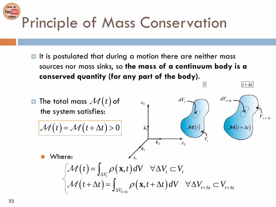
It is postulated that during a motion there are neither mass sources nor mass sinks, so the mass of a continuum body is a conserved quantity (for any part of the body).
The total mass of the system satisfies:
Where:
Principle of Mass Conservation
( ) ( ) 0t t t= + ∆ >M M
( )tM
( ) ( ),t
t tVt t dV V Vρ
∆= ∀∆ ⊂∫ xM
( ) ( ),t t
t t t tVt t t t dV V Vρ
+∆+∆ +∆∆
+ ∆ = + ∆ ∀∆ ⊂∫ xM
22
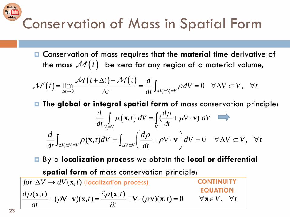
Conservation of mass requires that the material time derivative of the mass be zero for any region of a material volume,
The global or integral spatial form of mass conservation principle:
By a localization process we obtain the local or differential
spatial form of mass conservation principle:
Conservation of Mass in Spatial Form
( )tM
( ) ( ) ( )0
lim 0 ,t tV V Vt
t t t dt dV V V tt dt
ρ∆ ⊂ ≡∆ →
+ ∆ −′ = = = ∀∆ ⊂ ∀
∆ ∫M MM
( , ) 0 ,t tV V V V V
d dt dV dV V V tdt dt
ρρ ρ∆ ⊂ ≡ ∆ ⊂
= + ∇ ⋅ = ∀∆ ⊂ ∀ ∫ ∫x v
( , )( , ) ( , )( )( , ) ( )( , ) 0 ,
xx xv x v x x
for V dV td t tt t V t
dt tρ ρρ ρ
∆ →∂
+ ⋅ = + ⋅ = ∀ ∈ ∀∂
∇ ∇
(localization process) CONTINUITY EQUATION
( ), ( ) V V Vt
d dt dV dVdt dt
µµ µ≡
= + ∇ ⋅∫ ∫x v
23
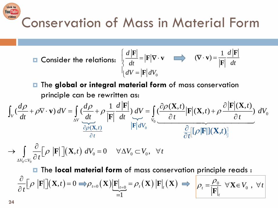
Consider the relations: The global or integral material form of mass conservation
principle can be rewritten as:
The local material form of mass conservation principle reads :
Conservation of Mass in Material Form
1( )F
vF
ddt
⋅ =∇
( )0 0
0
0
0 0 0
( , )1 ( , )( ) ( ) ( ( , ) )
, 0 ,
[ | |]( , )
VV V
V V
t
d td d tdV dV t dVdt dt dt t t
t dV V V tt
t
ρ ρ ρρ ρ ρ
ρ
ρ
∆
∆
⊂
∂∂
∂∂+ ∇ ⋅ = + = +
∂ ∂
∂→ = ∀∆ ⊂ ∀ ∂
∫ ∫ ∫
∫
F F XXv F XF
F X
F X
00 ,t
t
V tρρ = ∀ ∈ ∀XF
( ) ( )
( ) ( )0 0
1
, 0 t tt tt
tρ ρ ρ= =
=
∂= = ∂
F X X F X F X
24
( , )tt
ρ∂∂X 0dVF
0
FF v
F
ddt
dV dV
= ⋅
=
∇

25
Ch.5. Balance Principles
5.5. Reynolds Transport Theorem
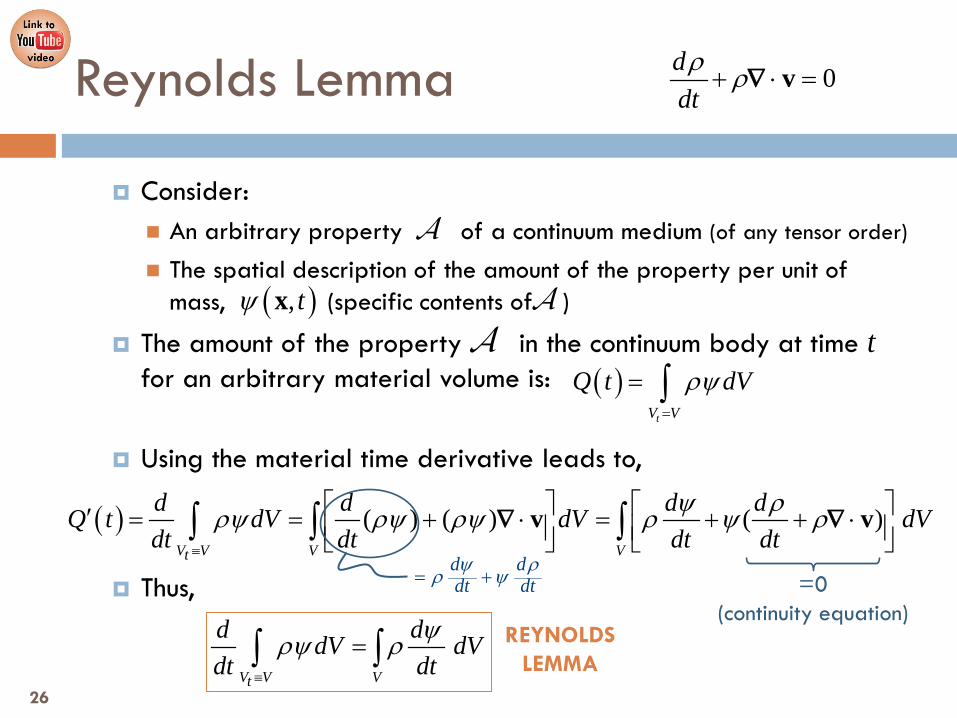
Consider: An arbitrary property of a continuum medium (of any tensor order)
The spatial description of the amount of the property per unit of mass, (specific contents of )
The amount of the property in the continuum body at time for an arbitrary material volume is:
Using the material time derivative leads to,
Thus,
Reynolds Lemma
A
( ), tψ xA
( )tV V
Q t dVρψ=
= ∫t
V V Vt
d ddV dVdt dt
ψρψ ρ≡
=∫ ∫ REYNOLDS LEMMA
0ddtρ ρ+ ⋅ =v∇
( ) ( ) ( ) ( ) V V V Vt
d d d dQ t dV dV dVdt dt dt dt
ψ ρρψ ρψ ρψ ρ ψ ρ≡
′ = = + ⋅ = + + ⋅ ∫ ∫ ∫v v∇ ∇
=0 (continuity equation)
d ddt dtψ ρρ ψ= +
26
A
V
dVρψ∫
V∂dV
ddtψρ
1e2e3e
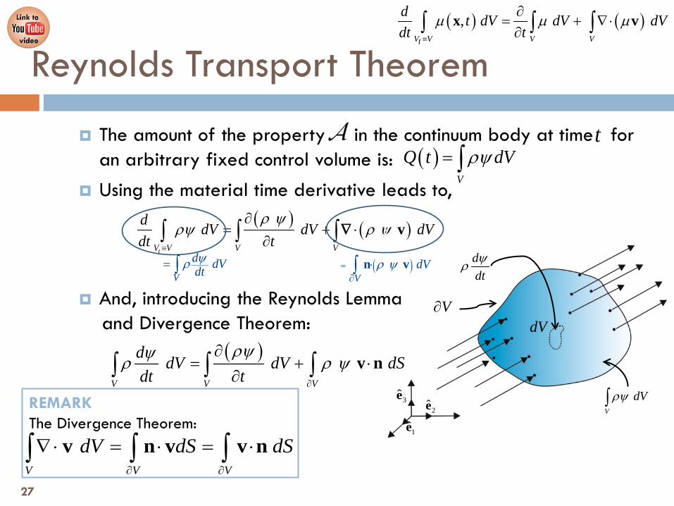
The amount of the property in the continuum body at time for an arbitrary fixed control volume is:
Using the material time derivative leads to,
And, introducing the Reynolds Lemma and Divergence Theorem:
Reynolds Transport Theorem
A( )
V
Q t dVρψ= ∫t
( ) ( )
tV V V V
d dV dV dVdt t
ρ ψρψ ρ ψ
≡
∂= + ⋅
∂∫ ∫ ∫ v∇
( ) v nV V V
d dV dV dSdt t
ρψψρ ρ ψ∂
∂= + ⋅
∂∫ ∫ ∫REMARK The Divergence Theorem:
v n v v nV V V
dV dS dS∂ ∂
∇ ⋅ = ⋅ = ⋅∫ ∫ ∫
( ) ( ), x vV V V Vt
d t dV dV dVdt t
µ µ µ≡
∂= + ∇ ⋅∂∫ ∫ ∫
;
( ) V
dVρ ψ=∂
⋅∫ n v V
d dVdtψρ= ∫
27
V
dVρψ∫
V∂dV
ddtψρ
1e2e3e
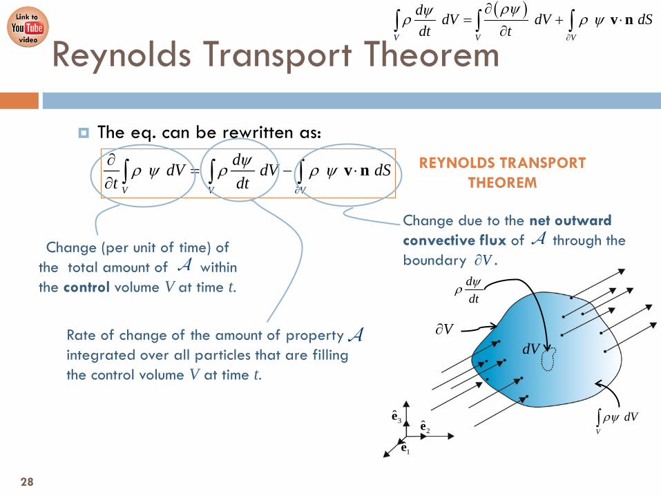
The eq. can be rewritten as:
Reynolds Transport Theorem
V V V
ddV dV dSt dt
ψρ ψ ρ ρ ψ∂
∂= − ⋅
∂ ∫ ∫ ∫ v n REYNOLDS TRANSPORT THEOREM
Change (per unit of time) of the total amount of . within the control volume V at time t.
A
Rate of change of the amount of property integrated over all particles that are filling the control volume V at time t.
A
Change due to the net outward convective flux of through the boundary .
A
( ) v nV V V
d dV dV dSdt t
ρψψρ ρ ψ∂
∂= + ⋅
∂∫ ∫ ∫
V∂
28

V
dVρψ∫
V∂
dV
ddtψρ
1e2e3e
Reynolds Transport Theorem
V V V
ddV dV dSt dt
ψρ ψ ρ ρ ψ∂
∂= − ⋅
∂ ∫ ∫ ∫ v n REYNOLDS TRANSPORT THEOREM (integral form)
V V V
ddV dV dSt dt
ψρ ψ ρ ρ ψ∂
∂= − ⋅
∂ ∫ ∫ ∫ v n
( ) ( )d V tt dt
ψρ ψ ρ ρ ψ∂= − ⋅ ∀ ∈ ∀
∂v x∇
REYNOLDS TRANSPORT THEOREM (local form)
( ) [ ( )] V V V V
ddV dV V V tt dt
ψρ ψ ρ ρ ψ∆ ⊂ ∆ ⊂
∂= − ⋅ ∀∆ ⊂ ∀
∂∫ ∫ v∇
( ) V
dVρ ψ= ⋅∫ v∇( ) V
dVtρ ψ∂
=∂∫
29

30
Ch.5. Balance Principles
5.6. General Balance Equation
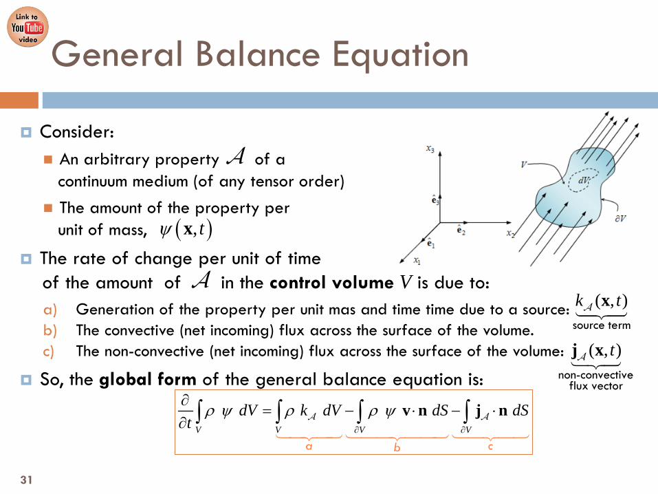
Consider: An arbitrary property of a continuum medium (of any tensor order) The amount of the property per unit of mass,
The rate of change per unit of time of the amount of in the control volume V is due to:
a) Generation of the property per unit mas and time time due to a source: b) The convective (net incoming) flux across the surface of the volume. c) The non-convective (net incoming) flux across the surface of the volume:
So, the global form of the general balance equation is:
General Balance Equation
A
( ), tψ x
V V V V
dV k dV dS dSt
ρ ψ ρ ρ ψ∂ ∂
∂= − ⋅ − ⋅
∂ ∫ ∫ ∫ ∫v n j n
A A
a cb
A( , )k tx
A
source term
( , )tj x
A
non-convectiveflux vector
31

The global form is rewritten using the Divergence Theorem and the definition of local derivative:
The local spatial form of the general balance equation is:
General Balance Equation
ddt kψρ ρ= − ⋅ jA A∇
( ) ( ) ( )
( )
V V
V V
V V V V
dV dSt
dV k dVt
d dV k dV V V tdt
ρ ψ ρ ψ
ρ ψ ρ ψ ρ
ψρ ρ
∂
∆ ⊂ ∆ ⊂
∂+ ⋅ =
∂
∂ = + ⋅ = − ⋅ ∂
= − ⋅ ∀∆ ⊂ ∀
∫ ∫
∫ ∫
∫ ∫
v n
v j
j
A A
A A
∇ ∇
∇
V V V V
dV k dV dS dSt
ρ ψ ρ ρ ψ∂ ∂
∂= − ⋅ − ⋅
∂ ∫ ∫ ∫ ∫v n j nA A
REMARK For only convective transport then and the variation of the contents of in a given particle is only due to the internal generation .
ddt kψρ ρ= A( )=j 0A
kρ A
ddtψρ= (Reynolds Theorem)
32

Example
If the property is associated to mass , then: The amount of the property per unit of mass is . The mass generation source term is .
The mass conservation principle states that mass cannot be generated.
The non-convective flux vector is . Mass cannot be transported in a non-convective form.
Then, the local spatial form of the general balance equation is:
A ≡A M1ψ =
1 1( ) ( ) 0d
dt tψρ ρ ψ ρ ψ
= =
∂= + ⋅ =∂
v∇
0k =M
0=jM
( ) 0tρ ρ∂+ ⋅ =
∂v∇
000d
dt kψρ ρ==
= − ⋅ =jA A∇
33
( ) 0d V tt dtρ ρρ ρ∂+ ⋅ = + ⋅ = ∀ ∈ ∀
∂v v x∇ ∇
Two equivalent forms of the continuity equation.
ddt kψρ ρ= − ⋅ jA A∇
( ) ( )d Vt dt
ψρψ ρ ρ ψ∂= − ⋅ ∀ ∈
∂v x∇
34
Ch.5. Balance Principles
5.7. Linear Momentum Balance
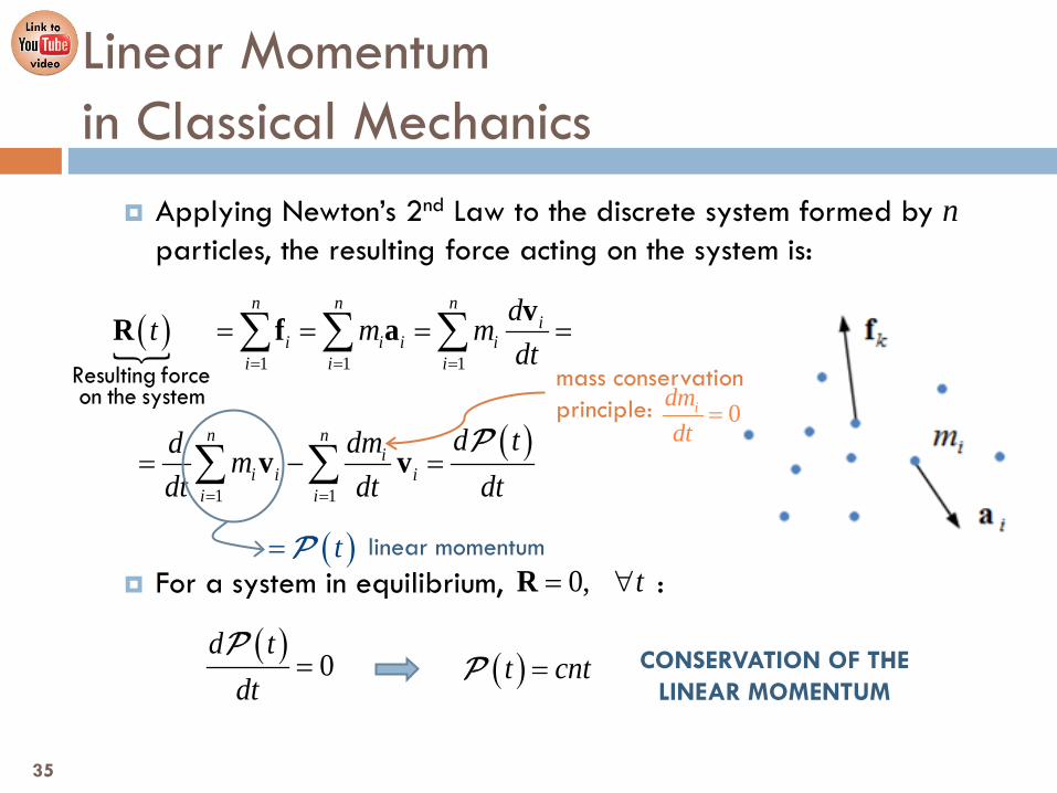
Applying Newton’s 2nd Law to the discrete system formed by n particles, the resulting force acting on the system is:
For a system in equilibrium, :
Linear Momentum in Classical Mechanics
( )
( )
1 1 1
1 1
n n ni
i i i ii i i
n ni
i i ii i
dt m mdt
d tdmd mdt dt dt
= = =
= =
= = = =
= − =
∑ ∑ ∑
∑ ∑
vR f a
v v
Resulting forceon the system
P
mass conservation principle: 0idm
dt=
0, t= ∀R
( ) 0d t
dt=
P( )t cnt=P CONSERVATION OF THE
LINEAR MOMENTUM
35
( )t=P linear momentum

The linear momentum of a material volume of a continuum medium with mass is:
Linear Momentum in Continuum Mechanics
MtV
( ) ( ) ( ) ( ), , ,V
t t d t t dVρ= =∫ ∫v x x v xM
MP
d dVρ=M
( )1
n
i ii
t m=
=∑ vP
36
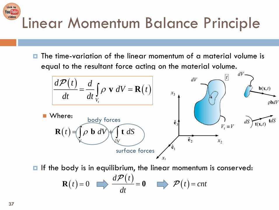
The time-variation of the linear momentum of a material volume is equal to the resultant force acting on the material volume. Where:
If the body is in equilibrium, the linear momentum is conserved:
Linear Momentum Balance Principle
( ) ( ) tV
d t d dV tdt dt
ρ= =∫ v RP
( ) V V
t dV dSρ∂
= +∫ ∫R b tbody forces
surface forces
( ) 0t =R( ) ( )d t
t cntdt
= =0P P
37

The global form of the linear momentum balance principle:
Introducing and using the Divergence Theorem,
So, the global form is rewritten:
Global Form of the Linear Momentum Balance Principle
( )
( )
( ) ,t tV V V V V V V
t
d tdt dV dS dV V V tdt dt
ρ ρ∆ ⊂ ∂∆ ⊂ ∆ ⊂ ≡
= + = = ∀∆ ⊂ ∀∫ ∫ ∫R b t v
P
P
= ⋅t n σ
V V V
dS dS dV∂ ∂
= ⋅ = ⋅∫ ∫ ∫t n σ ∇ σ
( )
+ ,t t
V V V V
V V V V V
dV dS
ddV dV V V tdt
ρ
ρ ρ
∆ ⊂ ∂∆ ⊂
∆ ⊂ ∆ ⊂ ≡
+ =
= ⋅ = ∀∆ ⊂ ∀
∫ ∫
∫ ∫
b t
b v∇ σ38
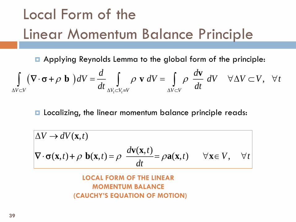
Applying Reynolds Lemma to the global form of the principle:
Localizing, the linear momentum balance principle reads:
Local Form of the Linear Momentum Balance Principle
( ) ,t tV V V V V V V
d ddV dV dV V V tdt dt
ρ ρ ρ∆ ⊂ ∆ ⊂ ≡ ∆ ⊂
⋅ = = ∀∆ ⊂ ∀∫ ∫ ∫vb v∇ σ +
( , )( , )( , ) ( , ) ( , ) ,
xv xx b x a x x
V dV td tt t t V t
dtρ ρ ρ
∆ →
⋅ = = ∀ ∈ ∀∇ σ +
LOCAL FORM OF THE LINEAR MOMENTUM BALANCE
(CAUCHY’S EQUATION OF MOTION)
39

40
Ch.5. Balance Principles
5.8. Angular Momentum Balance
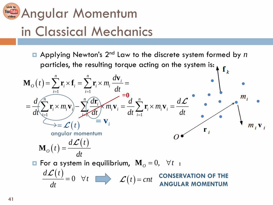
Applying Newton’s 2nd Law to the discrete system formed by n particles, the resulting torque acting on the system is:
For a system in equilibrium, :
Angular Momentum in Classical Mechanics
( )1 1
1 1 1
n ni
O i i i ii i
n n ni
i i i i i i i ii i i
dt mdt
dd d dm m mdt dt dt dt
= =
= = =
= × = × =
= × − × = × =
∑ ∑
∑ ∑ ∑
vM r f r
rr v v r v L
0,O t= ∀M( ) 0
d tt
dt= ∀
L( )t cnt=L CONSERVATION OF THE
ANGULAR MOMENTUM
i= v
=0
( ) ( )O
d tt
dt=M
L
41
( )t= Langular momentum

The angular momentum of a material volume of a continuum medium with mass is:
Angular Momentum in Continuum Mechanics
MtV
( )
( ) ( ) ( ), , ,V
t t d t t dVρ≡
= × = ×∫ ∫xr v x x x v x
M
ML
d dVρ=M
42
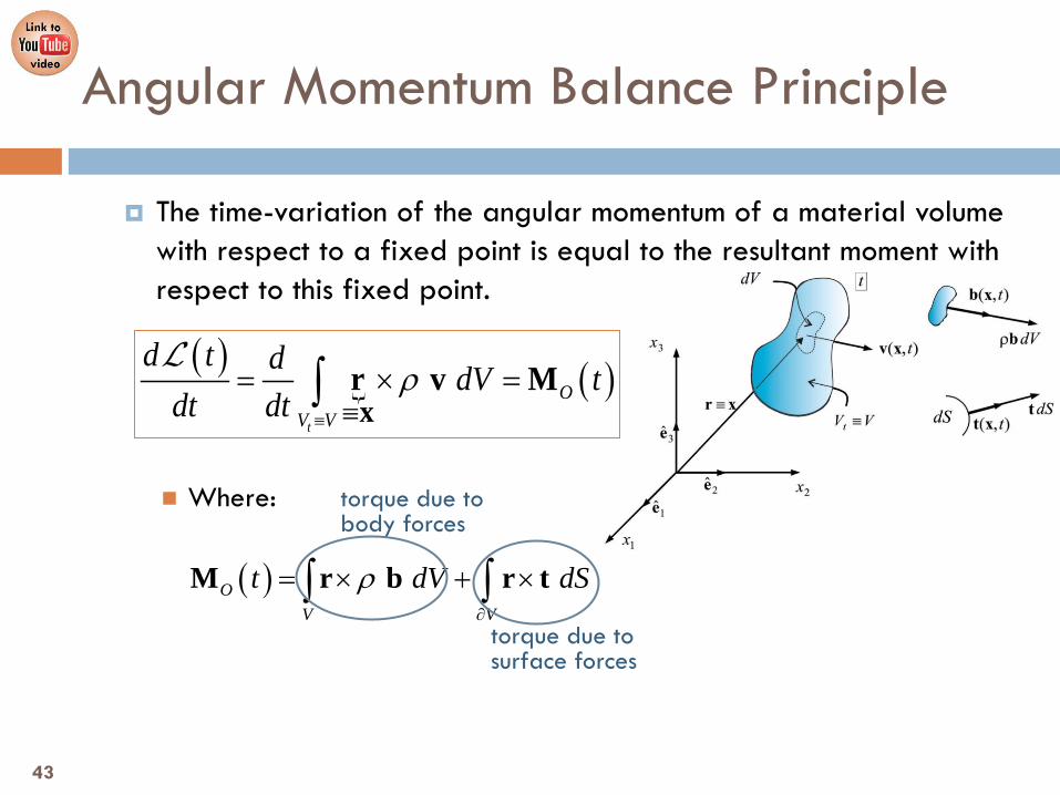
The time-variation of the angular momentum of a material volume with respect to a fixed point is equal to the resultant moment with respect to this fixed point.
Where:
Angular Momentum Balance Principle
( )
( ) t
OV V
d t d dV tdt dt
ρ≡ ≡
= × =∫ xr v M
L
( ) OV V
t dV dSρ∂
= × + ×∫ ∫M r b r t
torque due to body forces
torque due to surface forces
43

The global form of the angular momentum balance principle:
Introducing and using the Divergence Theorem,
It can be proven that,
Global Form of the Angular Momentum Balance Principle
( ) ( ) ( ) tV V V V
ddV dS dVdt
ρ ρ∂ ≡
× + × = ×∫ ∫ ∫r b r t r v
= ⋅t n σ
( )
( )
T T
V V V V
T
V
dS dS dS dS
dV∂ ∂ ∂ ∂
× = × ⋅ = × ⋅ = × ⋅ =
= × ⋅
∫ ∫ ∫ ∫
∫
r t r n r n r n
r
σ σ σ
σ ∇
( )ˆ ;
r r m
m e
T
i i i ijk jkm m σ
× ⋅ = ×∇ ⋅ +
= =
σ ∇ σREMARK is the Levi-Civita permutation symbol.
ijk
44

Applying Reynolds Lemma to the right-hand term of the global form equation:
Then, the global form of the balance principle is rewritten:
Global Form of the Angular Momentum Balance Principle
( ) ˆ vr b e rijk jk iV V
ddV dVdt
ρ σ ρ × +∇ ⋅ + = × ∫ ∫σ
( ) ( )
r v r v r v
r v vv r r
t tV V V V V
V V
d d ddV dV dVdt dt dt
d d ddV dVdt dt dt
ρ ρ ρ
ρ ρ
≡
↓
≡
× = × = × =
= × + × = ×
∫ ∫ ∫
∫ ∫
Reynold'sLemma
= v
=0
45
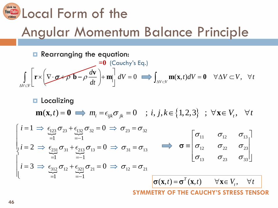
Rearranging the equation:
Localizing
Local Form of the Angular Momentum Balance Principle
0 ( , ) ,V V
V V
d dV t dV V V tdt
ρ ρ∆ ⊂
∆ ⊂
× ∇ ⋅ + + = = ∀∆ ⊂ ∀ ∫ ∫vr b m m x 0σ −
=0 (Cauchy’s Eq.)
{ }( , ) 0 ; , , 1, 2,3 ; ,m x 0 xi ijk jk tt m i j k V tσ= = = ∈ ∀ ∈ ∀
123 23 132 32 23 32
231 31 213 13 31 13
312 12 321 21 12 21
1 1
1 1
1 1
1 0
2 0
3 0
i
i
i
σ σ σ σ
σ σ σ σ
σ σ σ σ
= =−
= =−
= =−
⇒ ⇒
⇒ ⇒
⇒ ⇒
= + = = = + = == + = =
( , ) ( , ) ,Ttt t V t= ∀ ∈ ∀x x xσ σ
SYMMETRY OF THE CAUCHY’S STRESS TENSOR
11 12 13
12 22 23
13 23 33
σ σ σσ σ σσ σ σ
≡
σ
46

47
Ch.5. Balance Principles
5.9. Mechanical Energy Balance

Power, , is the work performed in the system per unit of time.
In some cases, the power is an exact time-differential of a function (then termed) energy :
It will be assumed that the continuous medium absorbs power from the exterior through: Mechanical Power: the work performed by the mechanical actions
(body and surface forces) acting on the medium. Thermal Power: the heat entering the medium.
Power
( )W t
( )( ) d tW tdt
=E
E
48
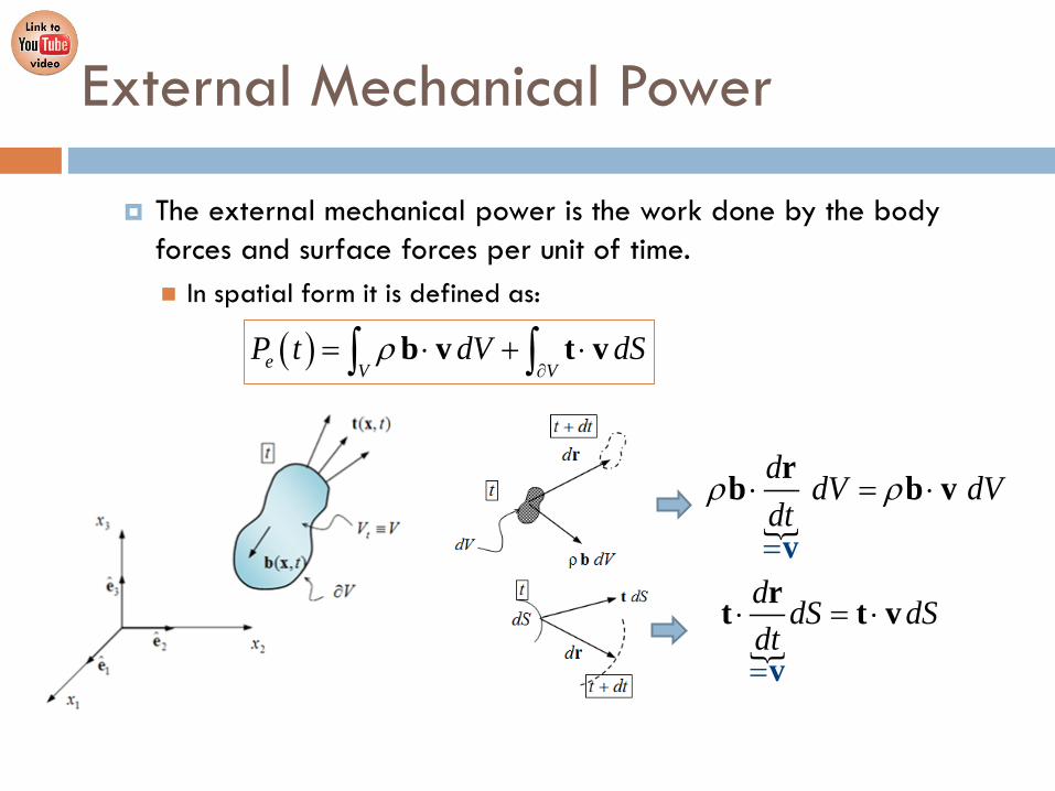
The external mechanical power is the work done by the body forces and surface forces per unit of time. In spatial form it is defined as:
External Mechanical Power
( )e V VP t dV dSρ
∂= ⋅ + ⋅∫ ∫b v t v
d dV dVdt
ρ ρ
=
⋅ = ⋅
v
rb b v
d dS dSdt=
⋅ = ⋅
v
rt t v

Using and the Divergence Theorem, the traction contribution reads,
Taking into account the identity:
So,
Mechanical Energy Balance
= ⋅t n σ
( ) ( ) ( ) :V V V V
dS dS dV dV∂ ∂
⋅⋅ = ⋅ ∇ ⋅ ⋅ =⋅ = ∇ ⋅ ⋅ + ∇ ∫ ∫ ∫ ∫
nv n vt v v v
σσσ σ σ
= lspatial velocity gradient tensor
skewsymmetric
= +l d w= +: l : d : wσ σ σ
=0
( ) :V V V
dS dV dV∂
⋅ = ⋅ ⋅ +∫ ∫ ∫t v v d∇ σ σ
50
↓
DivergenceTheorem

Substituting and collecting terms, the external mechanical power in spatial form is,
Mechanical Energy Balance
( ) ( )
( )
:
: :
V Ve V
V V V V
V
dV dV
dt
d
d
S
P t dV
ddV dV dV dVdt
ρ
ρ
ρ ρ
∂
∇ ⋅ ⋅
⋅
=
= ⋅ + + =
= ∇ ⋅ + ⋅ + = ⋅ +
∫∫ ∫∫
∫ ∫ ∫ ∫
v d
v
t v
b v
vb v d v d
σ σ
σ σ σ
2
v
1 1( ) ( v )2 2
d ddt dt
ρρ=
= ⋅ =v
v v
( ) 2 21 1( v ) ( v ) 2 2e
V V V V
d dP t dV dV dV dVdt dt
ρ ρ↓
= + = +∫ ∫ ∫ ∫: d : d
Reynold'sLemma
σ σ
ddt
ρ ρ⋅ =vb∇ σ +
51

Mechanical Energy Balance. Theorem of the expended power. Stress power
( ) 21 v 2
t
e V VV V V
dP t dV dS dV dVdt
ρ ρ∂
≡
= ⋅ + ⋅ = +∫ ∫ ∫ ∫b v t v : dσ
external mechanical power entering the medium stress power kinetic energy
( ) ( )edP t t Pdt σ= +K
REMARK The stress power is the mechanical power entering the system which is not spent in changing the kinetic energy. It can be interpreted as the work by unit of time done by the stress in the deformation process of the medium. A rigid solid will produce zero stress power ( ) .
K
=d 0
Pσ
52
Theorem of the expended mechanical power

The external thermal power is incoming heat in the continuum medium per unit of time.
The incoming heat can be due to: Non-convective heat transfer across the volume’s surface.
Internal heat sources
External Thermal Power
( , ) V
t dS∂
− ⋅ =∫ q x n
heat conduction flux vector
incoming heatunit of time
( , )V
r t dVρ =∫ x
specific internal heat production
heat generated by internal sourcesunit of time
53
The external thermal power is incoming heat in the continuum medium per unit of time. In spatial form it is defined as:
where:
is the non-convective heat flux vector per unit of spatial surface is the internal heat source rate per unit of mass.
External Thermal Power
( )
)
( )
n q
q
q n qeV V V
V
V
dS
dV
Q t r dV dS r dVρ ρ∂
∂= ⋅
= ⋅
= − ⋅ = − ⋅
∫∫
∫ ∫ ∫
(∇
∇
( ),r tx( ), tq x
54
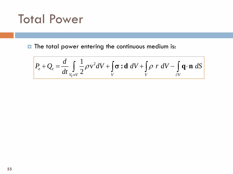
The total power entering the continuous medium is:
Total Power
21 v 2e e
V V V V Vt
dP Q dV dV r dV dSdt
ρ ρ≡ ∂
+ = + + − ⋅∫ ∫ ∫ ∫: d q nσ
55

56
Ch.5. Balance Principles
5.10. Energy Balance
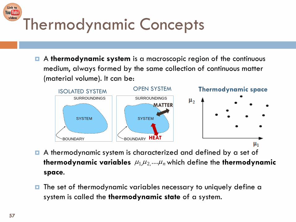
A thermodynamic system is a macroscopic region of the continuous medium, always formed by the same collection of continuous matter (material volume). It can be:
A thermodynamic system is characterized and defined by a set of thermodynamic variables which define the thermodynamic space.
The set of thermodynamic variables necessary to uniquely define a system is called the thermodynamic state of a system.
Thermodynamic Concepts
HEAT
MATTER
ISOLATED SYSTEM OPEN SYSTEM
1, 2, .... nµ µ µ
57
Thermodynamic space

A thermodynamic process is the energetic development of a thermodynamic system which undergoes successive thermodynamic states, changing from an initial state to a final state
→ Trajectory in the thermodynamic space. If the final state coincides with the initial state, it is a closed cycle process.
A state function is a scalar, vector or tensor entity defined univocally as a function of the thermodynamic variables for a given system. It is a property whose value does not depend on the path taken to reach that
specific value.
Thermodynamic Concepts
58

Is a function uniquely valued in terms of the “thermodynamic state” or, equivalently, in terms of the thermodynamic variables
Consider a function , that is not a state function, implicitly defined in the thermodynamic space by the differential form:
The thermodynamic processes and yield:
For to be a state function, the differential form must be an exact differential: , i.e., must be integrable:
The necessary and sufficient condition for this is the equality of cross-derivatives:
State Function
( )1 2,φ µ µ{ }1 2, , , nµ µ µ
( ) ( )1 1 2 1 2 1 2 2, , f d f dδφ µ µ µ µ µ µ= +
1 1'
1 2
2 2
2 1 2 2
' 2 1 2 2
( , )
( , )
B A
BB
B A
f
f
φ φ δφ µ µ δµδφ δφ φ φ
φ φ δφ µ µ δµ
Γ Γ
Γ Γ
Γ Γ
= + = ≠ ≠ = + =
∫ ∫∫ ∫
∫ ∫
( ) ( ) { }11 ,...,,...,, 1,...j ni n
j i
ffi j n
µ µµ µµ µ
∂∂= ∀ ∈
∂ ∂dδφ φ=
59
( )1,..., nφ µ µ
1Γ 2Γ
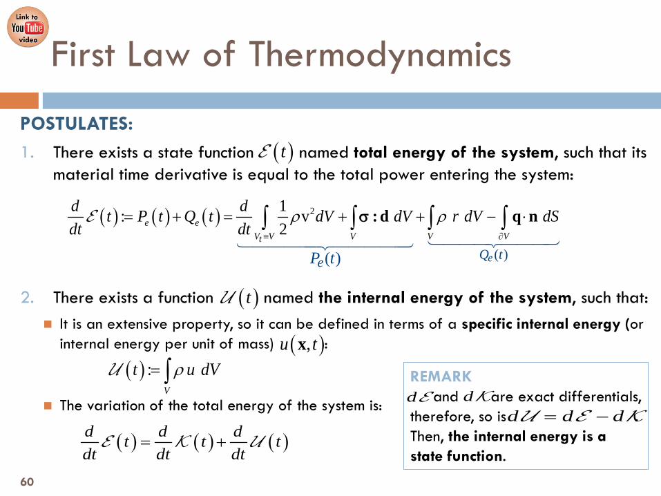
POSTULATES: 1. There exists a state function named total energy of the system, such that its
material time derivative is equal to the total power entering the system:
2. There exists a function named the internal energy of the system, such that: It is an extensive property, so it can be defined in terms of a specific internal energy (or
internal energy per unit of mass) :
The variation of the total energy of the system is:
First Law of Thermodynamics
( )tE
( ) ( ) ( ) 2
( )( )
1: v 2e e
V V V V Vt
eQ teP t
d dt P t Q t dV dV r dV dSdt dt
ρ ρ≡ ∂
= + = + + − ⋅∫ ∫ ∫ ∫: d q n
E σ
( )tU
( ),u tx( ) :
V
t u dVρ= ∫U
( ) ( ) ( )d d dt t tdt dt dt
= +E K U
REMARK and are exact differentials, therefore, so is . Then, the internal energy is a state function.
dKdEd d d= −U E K
60
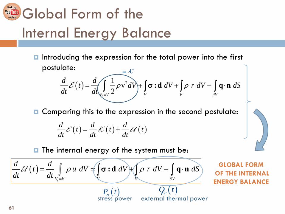
Introducing the expression for the total power into the first postulate:
Comparing this to the expression in the second postulate:
The internal energy of the system must be:
Global Form of the Internal Energy Balance
( ) 21 v 2V V V V Vt
d dt dV dV r dV dSdt dt
ρ ρ≡ ∂
= + + − ⋅∫ ∫ ∫ ∫: d q nE σ
=K
( ) tV V V V V
d dt u dV dV r dV dSdt dt
ρ ρ≡ ∂
= = + − ⋅∫ ∫ ∫ ∫: d q nU σ GLOBAL FORM OF THE INTERNAL ENERGY BALANCE
, external thermal power
( )eQ t stress power
( )P tσ
61
( ) ( ) ( )d d dt t tdt dt dt
= +E K U
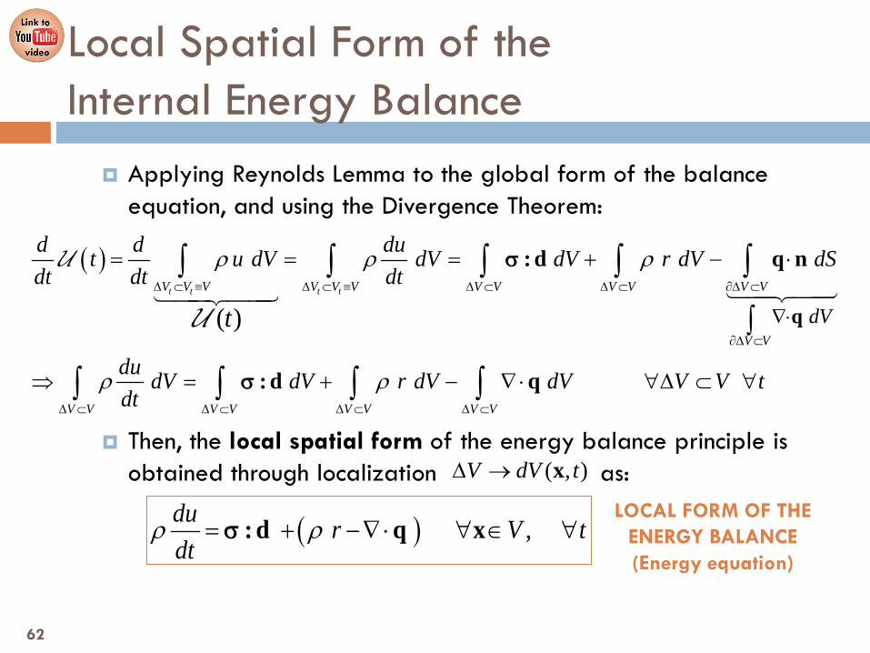
Applying Reynolds Lemma to the global form of the balance equation, and using the Divergence Theorem:
Then, the local spatial form of the energy balance principle is obtained through localization as:
Local Spatial Form of the Internal Energy Balance
( ) ,du r V tdt
ρ ρ= + −∇⋅ ∀ ∈ ∀: d q xσLOCAL FORM OF THE
ENERGY BALANCE (Energy equation)
( )
( )t t t tV V V V V V V V V V V V
V V V V V V V V
V VdV
d d dut u dV dV dV r dV dSdt dt dt
du dV dV r dV dV V V tdt
t
ρ ρ ρ
ρ ρ
∆ ⊂ ≡ ∆ ⊂ ≡ ∆ ⊂ ∆ ⊂ ∂∆ ⊂
∆ ⊂ ∆ ⊂ ∆ ⊂ ∆ ⊂
∂∆ ⊂
∇⋅
= = = + − ⋅
⇒ = + − ∇⋅ ∀∆ ⊂ ∀
∫
∫ ∫ ∫ ∫ ∫
∫ ∫ ∫ ∫
q
: d q n
: d q
U
U
σ
σ
62
( , )V dV t∆ → x

The total energy is balanced in all thermodynamics processes following: In an isolated system (no work can enter or exit the system)
However, it is not established if the energy exchange can happen in both senses or not:
There is no restriction indicating if an imagined arbitrary process is
physically possible or not.
Second Law of Thermodynamics
( ) ( )e ed d dP t Q tdt dt dt
+ = = +E K U
( ) ( ) 0e edP t Q tdt
+ = =E 0d d
dt dt+ =
U K
0 0d ddt dt
< >U K0 0d d
dt dt> <
U K
63

If a brake is applied on a spinning wheel, the speed is reduced due to the conversion of kinetic energy into heat (internal energy). This process never occurs the other way round.
Spontaneously, heat always flows to regions of lower temperature, never to regions of higher temperature.
Second Law of Thermodynamics
The concept of energy in the first law does not account for the observation that natural processes have a preferred direction of progress. For example:
0 0d ddt dt
> <U K
64 18/11/2016 MMC - ETSECCPB - UPC
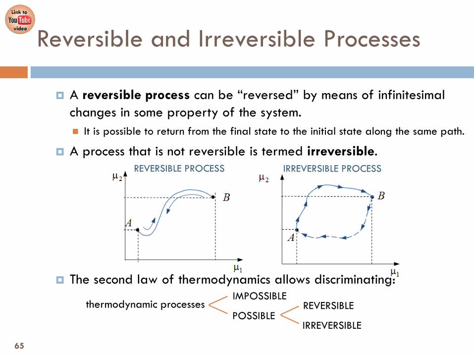
A reversible process can be “reversed” by means of infinitesimal changes in some property of the system. It is possible to return from the final state to the initial state along the same path.
A process that is not reversible is termed irreversible.
The second law of thermodynamics allows discriminating:
Reversible and Irreversible Processes
REVERSIBLE PROCESS IRREVERSIBLE PROCESS
65
REVERSIBLE
IRREVERSIBLE
IMPOSSIBLE
POSSIBLE thermodynamic processes
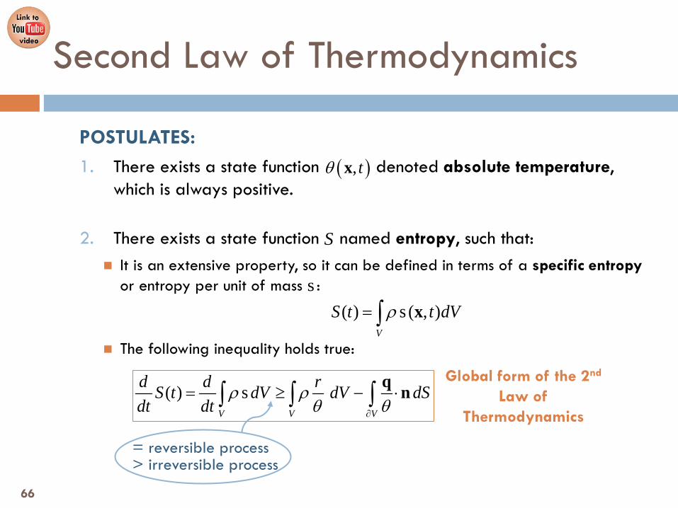
POSTULATES: 1. There exists a state function denoted absolute temperature,
which is always positive.
2. There exists a state function named entropy, such that: It is an extensive property, so it can be defined in terms of a specific entropy
or entropy per unit of mass :
The following inequality holds true:
Second Law of Thermodynamics
( ), tθ x
S
s( ) s ( , )
V
S t t dVρ= ∫ x
( ) sV V V
d d rS t dV dV dSdt dt
ρ ρθ θ∂
= ≥ − ⋅∫ ∫ ∫q n
Global form of the 2nd Law of
Thermodynamics
= reversible process > irreversible process
66
Second Law of Thermodynamics
( ) sV V V
d d rS t dV dV dSdt dt
ρ ρθ θ∂
= ≥ − ⋅∫ ∫ ∫q n
Global form of the 2nd Law of
Thermodynamics
= reversible process > irreversible process
( ) eV V
Q t r dV dSρ∂
= − ⋅∫ ∫ q nrate of the total amount of the entity heat, per unit of time, (external thermal power) entering into the system
( ) eV V
rt dV dSρθ θ∂
Γ = − ⋅∫ ∫q n
rate of the total amount of the entity heat per unit of absolute temperature, per unit of time (external heat/unit of temperature power) entering into the system
( )e t= Γ
67
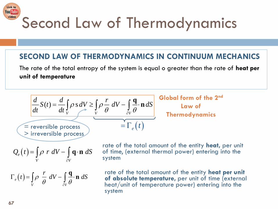
SECOND LAW OF THERMODYNAMICS IN CONTINUUM MECHANICS The rate of the total entropy of the system is equal o greater than the rate of heat per unit of temperature

Consider the decomposition of entropy into two (extensive) counterparts: Entropy generated inside the continuous medium:
Entropy generated by interaction with the outside medium:
Second Law of Thermodynamics
( ) ( ) ( )s ,i i
V
S t dVρ= ∫ x
( ) ( ) ( )s ,e e
V
S t dVρ= ∫ x
( ) ( ) ( ) ( ) ( )( ) ( )
i e
i e
S t S t S t
dS dS dSdt dt dt
= +
= +
68
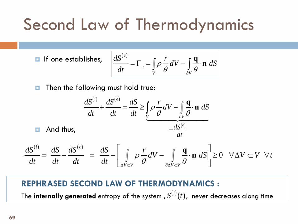
If one establishes,
Then the following must hold true:
And thus,
Second Law of Thermodynamics
( ) ( ) 0
i e
V V V V
dS dS dS dS r dV dS V V tdt dt dt dt
ρθ θ∆ ⊂ ∂∆ ⊂
= − = − − ⋅ ≥ ∀∆ ⊂ ∀
∫ ∫
q n
( )
e
eV V
dS r dV dSdt
ρθ θ∂
= Γ = − ⋅∫ ∫q n
( ) ( )
( )
i e
V V
edSdt
dS dS dS r dV dSdt dt dt
ρθ θ∂
=
+ = ≥ − ⋅∫ ∫q n
69
REPHRASED SECOND LAW OF THERMODYNAMICS : The internally generated entropy of the system , , never decreases along time ( ) ( )iS t
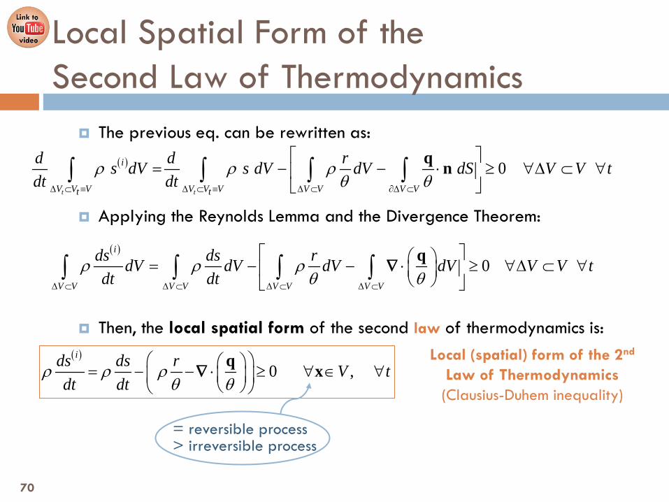
The previous eq. can be rewritten as:
Applying the Reynolds Lemma and the Divergence Theorem:
Then, the local spatial form of the second law of thermodynamics is:
Local Spatial Form of the Second Law of Thermodynamics
( ) 0t t
i
V V V V V V V V V Vt t
d d rs dV s dV dV dS V V tdt dt
ρ ρ ρθ θ∆ ⊂ ≡ ∆ ⊂ ≡ ∆ ⊂ ∂∆ ⊂
= − − ⋅ ≥ ∀∆ ⊂ ∀
∫ ∫ ∫ ∫
q n
( )0
i
V V V V V V V V
ds ds rdV dV dV dV V V tdt dt
ρ ρ ρθ θ∆ ⊂ ∆ ⊂ ∆ ⊂ ∆ ⊂
= − − ⋅ ≥ ∀∆ ⊂ ∀
∫ ∫ ∫ ∫q
∇
( )0 ,
ids ds r V tdt dt
ρ ρ ρθ θ
= − − ⋅ ≥ ∀ ∈ ∀
q x∇
= reversible process > irreversible process
70
Local (spatial) form of the 2nd Law of Thermodynamics (Clausius-Duhem inequality)

Considering that,
The Clausius-Duhem inequality can be written as
Local Spatial Form of the Second Law of Thermodynamics
2
1 1( ) θθ θ θ
⋅ = ⋅ − ⋅q q q∇ ∇ ∇
( )
2
1 1 0ids ds r
dt dtθ
θ ρθ ρθ
= − + ⋅ − ⋅ ≥
q q∇ ∇
( )is= s=
( )ilocals= ( )i
conds=
REMARK (Stronger postulate) Internally generated entropy can be generated locally, , or by thermal conduction, , and both must be non-negative.
( )iconds
( )ilocals
Because density and absolute temperature are always positive, it is deduced that , which is the mathematical expression for the fact that heat flows by conduction from the hot parts of the medium to the cold ones.
0θ⋅ ≤q ∇
1 0rsθ ρθ
− + ⋅ ≥
q ∇
CLAUSIUS-PLANCK INEQUALITY 2
1 0θρθ
− ⋅ ≥q ∇
HEAT FLOW INEQUALITY
71
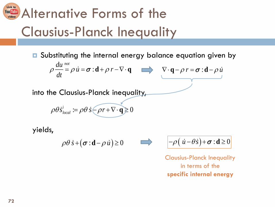
Substituting the internal energy balance equation given by
into the Clausius-Planck inequality,
yields,
Alternative Forms of the Clausius-Planck Inequality
:notdu u r
dtρ ρ ρ= = + −∇⋅d q σ
: 0ilocals s rρθ ρθ ρ= − +∇⋅ ≥q
( ) : 0u sρ θ− − + ≥d σ
:r uρ ρ∇⋅ − = −q d σ
( ): 0s uρθ ρ+ − ≥d σ
Clausius-Planck Inequality in terms of the
specific internal energy
72

74
Ch.5. Balance Principles
5.11. Governing Equations

Conservation of Mass. Continuity Equation.
1 eqn.
Governing Equations in Spatial Form
0ρ ρ+ ∇⋅ =v
Linear Momentum Balance. First Cauchy’s Motion Equation.
3 eqns. ρ ρ∇⋅ + =b vσ
Angular Momentum Balance. Symmetry of Cauchy Stress Tensor.
3 eqns. T=σ σ
Energy Balance. First Law of Thermodynamics.
1 eqn. :u rρ ρ= + −∇⋅d q σ
Second Law of Thermodynamics. Clausius-Planck Inequality.
Heat flow inequality 2 restrictions
( ) 0u sρ θ− − + ≥: d σ
2
1 0θρθ
− ⋅ ≥q ∇8 PDE + 2 restrictions
75

The fundamental governing equations involve the following variables:
At least 11 equations more (assuming they do not involve new unknowns), are needed to solve the problem, plus a suitable set of boundary and initial conditions.
Cauchy’s stress tensor field
Governing Equations in Spatial Form
v
σ
u
θ
s
q
density 1 variable ρ
velocity vector field 3 variables
9 variables
specific internal energy 1 variable
absolute temperature
heat flux per unit of surface vector field 3 variables
1 variable
specific entropy 1 variable 19 scalar unknowns
76

Thermo-Mechanical Constitutive Equations. 6 eqns.
Constitutive Equations in Spatial Form
Thermal Constitutive Equation. Fourier’s Law of Conduction. 3 eqns.
State Equations. (1+p) eqns.
(19+p) PDE + (19+p) unknowns
( ), ,θ= vσ σ ζ
( ), ,s s θ= v ζ 1 eqn.
( ), Kθ θ= = −q q v ∇
( ) { }, , 0 1,2,...,iF i pρ θ = ∈ζ( ), , ,u f ρ θ= v ζ
Kinetic Heat
Entropy Constitutive Equation.
set of new thermodynamic variables: . { }1 2, ,..., p=ζ ζ ζ ζ
REMARK 1 The strain tensor is not considered an unknown as they can be obtained through the motion equations, i.e., . ( )= vε ε
REMARK 2 These equations are specific to each material.
77

Conservation of Mass. Continuity Mass Equation.
1 eqn.
The Coupled Thermo-Mechanical Problem
0ρ ρ+ ∇⋅ =v
Linear Momentum Balance. First Cauchy’s Motion Equation.
3 eqns.
Energy Balance. First Law of Thermodynamics.
1 eqn.
Second Law of Thermodynamics. Clausius-Planck Inequality.
2 restrictions.
Mechanical constitutive equations. 6 eqns. ( ( ), )θvσ = σ ε
16 scalar unknowns
10 equations
MMC - ETSECCPB - UPC 78

The mechanical and thermal problem can be uncoupled if
The temperature distribution is known a priori or does not intervene in the mechanical constitutive equations.
Then, the mechanical problem can be solved independently.
The Uncoupled Thermo-Mechanical Problem
( ), tθ x
79

Conservation of Mass. Continuity Mass Equation.
1 eqn.
The Uncoupled Thermo-Mechanical Problem
0ρ ρ+ ∇⋅ =v
Linear Momentum Balance. First Cauchy’s Motion Equation.
3 eqns.
Energy Balance. First Law of Thermodynamics.
1 eqn.
Second Law of Thermodynamics. Clausius-Planck Inequality.
2 restrictions.
Mechanical problem
Thermal problem
Mechanical constitutive equations. 6 eqns.
10 scalar unknowns
( ( ), θvσ = σ ε )
80
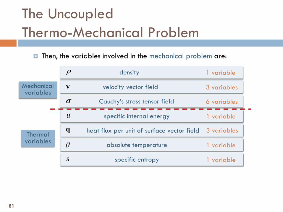
Then, the variables involved in the mechanical problem are:
The Uncoupled Thermo-Mechanical Problem
Cauchy’s stress tensor field
v
σ
density 1 variable ρ
velocity vector field 3 variables
6 variables
u
θ
s
q
specific internal energy 1 variable
absolute temperature
heat flux per unit of surface vector field 3 variables
1 variable
specific entropy 1 variable
Mechanical variables
Thermal variables
81