1-1

1. BASIC SOIL AND ROCK CHARACTERISTICS

1.1. THE PHASE DIAGRAM

Soils are normally composed of three constituents - solid soil particles, air and

water. The air and water occupy the void spaces or pores between the solid particles. In

the case of saturated soils the pore fluid is made up entirely of water.

To facilitate calculations involving various amounts of the three constituents of a

soil it is convenient to represent these constituents by means of a diagram, often known as

a phase diagram , as illustrated in Fig.1.1. The symbols for the masses and volumes of

the constituents are also shown on this figure. The mass of the air occupying the voids is

ignored since it is negligible by comparison with the masses of water and solid.

A number of definitions may now be given in terms of the symbols in Fig.1.1.

Bulk Density ρ = MW + MS

VA + VW + Vs (1.1)

(Sometimes referred to as total density ρt)

Dry Density ρd = Ms

VA + VW + Vs (1.2)

Density of Water ρw = MW

VW (1.3)

ρw is commonly taken as 1000 kg/m3 for convenience

Volume of Voids Vv = VA + VW (1.4)

Void Ratio e = VV

VS (1.5)

Porosity n = VV

VV + VS =

e

1 + e , (1.6)

often expressed as a percentage.

Degree of Saturation S or Sr = VW

VA + VW. (1.7)

usually expressed as a percentage.

1-2

Fig.1.1 Phase diagram for a partly Saturated soil

Fig.1.2 Phase diagram for a Saturated soil

Fig.1.3

Volume

water

solid

air

Mass

MW

MS

VA

VW

VS

Volume

water

solid

Mass

MW

MS

VW

VS

Volume

water

solid

air

Mass

MW

MS

VA

VW

VS

0.0

25

m3

45

.0 k

g

1-3

Density of Solid Particles or Soil Particle Density

ρs = Ms

Vs (1.8)

Specific Gravity of Solid Particles

G = ρs

ρw (1.9)

Water Content or Moisture Content

w = MW

MS , (1.10)

usually expressed as a percentage.

Air Voids Va = VA

VA + VW + VS , (1.11)

usually expressed as a percentage.

With a saturated soil the volume of air becomes zero as illustrated in Fig.1.2.

Referring to the figure a further definition can be given.

Saturated Density ρsat = MW + MS

VW + VS (1.12)

Example

A soil sample having a total volume of 0.025mm3 and total mass of 45.0 kg. has

been removed from the ground. If the water content and specific gravity of the soil are

20.0% and 2.68 respectively calculate:

a) the dry density of the sample,

b) the degree of saturation,

c) the porosity.

Referring to the phase diagram in Fig.1.3 the unknown terms MS, MW, VA, VW,

VS can be calculated as follows:

MW = w x MS = 0.20MS

but MW + MS = 45.0 kg

∴ 1.20MS = 45.0

∴ MS = 37.5 kg

∴ MW = 45.0 - 37.5 = 7.5 kg

1-4

The volumes can now be calculated

VW = MW

ρw =

7.5

1000 = .0075 m3

VS = MS

Gρw =

37.5

2.68 x 1000 = 0.014 m3

∴ VA = .025 - .014 - .0075 = .0035 m3

With these known quantitites the three items required can now be determined:

a) dry density ρd = MS

VA + VW + VS (1.2)

= 37.5

.025 = 1500 kg/m3

b) degree of saturation S = VW

VA + VW (1.7)

= .0075

.0035 + .0075 = 0.682 or 68.2%

c) porosity n = VA + VW

VA + VW + VS

= .0035 + .0075

.025 = 0.440 or 44.0%

1.2 IDENTIFICATION OF SOILS

In addition to the techniques described in Geomechanics 2 for identification of

the mineralogical components of soils, a number of relatively simple laboratory tests

which are useful in identifying various soil types, has been developed. The presentation

here will concentrate on grain size and plasticity characteristics, but reference should be

made to books on soil testing for details of the testing procedures. (Bowles, 1970,

Lambe, 1951, Kezdi, 1980). More sophisticated laboratory tests, which may be used for

soil identification are used on occasions but these will not be discussed in this

introductory presentation.

1.2.1 GRAIN SIZE DISTRIBUTION

Soils are traditionally described by one or more of the names gravel, sand, silt or

clay which indicate sizes of the soil particles. A number of slightly different

1-5

classification systems are in use relating size ranges to these four names but probably the

most widely used is the M.I.T. system as follows:

Gravel - grain size greater than 2mm

Sand - 0.06 mm to 2 mm

Silt - 0.002 mm to 0.06 mm

Clay - grain size less than 0.002 mm

Soils often consist of mixtures of these four ranges resulting in names such as silty

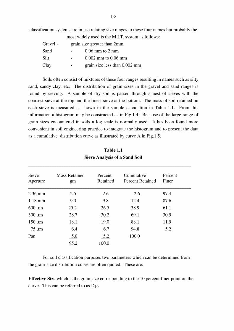
sand, sandy clay, etc. The distribution of grain sizes in the gravel and sand ranges is

found by sieving. A sample of dry soil is passed through a nest of sieves with the

coarsest sieve at the top and the finest sieve at the bottom. The mass of soil retained on

each sieve is measured as shown in the sample calculation in Table 1.1. From this

information a histogram may be constructed as in Fig.1.4. Because of the large range of

grain sizes encountered in soils a log scale is normally used. It has been found more

convenient in soil engineering practice to integrate the histogram and to present the data

as a cumulative distribution curve as illustrated by curve A in Fig.1.5.

Table 1.1

Sieve Analysis of a Sand Soil

_____________________________________________________________________

Sieve Mass Retained Percent Cumulative Percent

Aperture gm Retained Percent Retained Finer

_____________________________________________________________________

2.36 mm 2.5 2.6 2.6 97.4

1.18 mm 9.3 9.8 12.4 87.6

600 µm 25.2 26.5 38.9 61.1

300 µm 28.7 30.2 69.1 30.9

150 µm 18.1 19.0 88.1 11.9

75 µm 6.4 6.7 94.8 5.2

Pan 5.0 5.2 100.0

95.2 100.0

For soil classification purposes two parameters which can be determined from

the grain-size distribution curve are often quoted. These are:

Effective Size which is the grain size corresponding to the 10 percent finer point on the

curve. This can be referred to as D10.

1-6

Fig. 1.4 Histogram from a Sieve Analysis

Fig. 1.5 Grain size distribution curves

1-7

Uniformity Coefficient (Cu) which is a measure of the uniformity of grain size in the

soil and is defined as the ratio of the 60% finer size (D60) to D10.

that is Cu = D60

D10 (1.13)

For curve A in Fig.1.5 the uniformity coefficient is:

Cu = 0.57

0.14 = 4.1

which indicates a relatively uniform soil (sometimes referred to as poorly graded).

A grain size distribution curve for a soil with a uniformity coefficient larger than

that for soil A in Fig.1.5 is illustrated by curve B (well graded soil) in Fig.1.5. For the

silty clay soil represented by curve C in Fig.1.5 it is not possible to determine the

uniformity coefficient since the effective size is unknown.

Coefficient of Cuvature (Cc) is a value that can be used to identify a poorly graded soil.

6010

2

30

.

)(

DD

DCc = (1.14)

A well graded soil has Cc between 1 and 3 as long as Cu is also greater than 4 for gravels

and 6 for sands.

The finer portions of the grain size curves B and C cannot be determined by

sieving since a sieve with an aperture of about 75 µm is normally the finest sieve used in

this type of test. For silt and clay size soils the grain size distributions are found by

means of a sedimentation procedure in which a sample of the soil is allowed to settle in

water. This procedure utilizes Stokes Law which relates the size of a sphere to its fall

velocity in a fluid (usually water) by means of the expression:

D2 = 18000 η v

g(Gs - Gw) (1.15)

where D is the sphere diameter in mm

η is the dynamic viscosity of water in N sec/m2

v is the fall velocity of the sphere in cm/sec.

g is the gravitational acceleration in cm/sec2.

Gs is the specific gravity of the sphere solid

Gw is the specific gravity of the water.

1-8

The concentration of solids in the water at a particular time after the

commencement of sedimentation is found by measuring the specific gravity of the

suspension with an hydrometer. Alternatively the concentration may be found by taking a

small volume of suspension from a particular depth by means of a pipette. The mass of

solids is determined by drying off the water.

During preparation of the suspension for a sedimentation (or hydrometer) test a

deflocculating agent such as sodium hexametaphosphate or sodium silicate is

customarily added to prevent the formation of soil flocs. Some clay soils behave in such

a way that a variety of grain size distribution curves may be obtained depending upon the

type and concentration of deflocculating agent that is used. Discussion of the

recommended procedure for determining the grain size distribution of soils is given in the

S.A.A. Standard AS1289.

1.2.2 SOIL PLASTICITY

Changes in soil water content can produce significant changes in soil behaviour.

It is not surprising therefore to find that two widely used identification tests involve

observations of soil behaviour at two different water contents. In these tests water

contents, known as the Atterberg Limits, at which particular soil characteristics develop

are measured.

The larger water content, known as the Liquid Limit (wl) is the water content at

which the soil flows in a specially made cup when subjected to a series of small blows.

The liquid limit device permits the cup containing the soil in which a small groove has

been cut, to be lifted and dropped a small distance. The liquid limit is the water content

at which the groove closes when the soil has been subjected to 25 blows. The test is

performed by counting the number of blows to close the groove at various water contents.

The results are then plotted on a diagram such as Fig.1.6, from which the liquid limit may

be interpolated. The liquid limit may be estimated from the results of a test at a single

value of water content (w). If the number of blows for this test is n then the following

expression can be used to provide an estimate of wl.

wl = w(n

25 )0.121 (1.16)

For many Australian soils the following expression has been found to provide a

better estimate of wl.

wl = w(n

25 )0.091 (1.17)

1-9

Small laboratory cone penetrometers are increasingly being used for the

measurement of liquid limit. The British (BS 1377-1975) device for example is 35mm

long cone and has a 30o tip and a mass of 80 g. The liquid limit is taken to be the water

content of the soil when the penetration of this cone is 20 mm.

The smaller water content, known as the Plastic Limit (wp) is the water content at which

small threads of the soil crumble when rolled to a diameter of 3mm.

Fig. 1.6 Flow curve for Liquid Limit determination

These two tests are conducted on clayey and silty soils. These tests cannot be

conducted on granular soils such as sands and gravels. (See S.A.A. Standard AS1289).

The typical liquid and plastic limits for some clay soils are illustrated in Table 1.2 which

demonstrates the magnitude of the influence of the adsorbed cation as well as the type of

clay mineral.

1-10

TABLE 1.2

Typical Atterberg Limits for some Clay Soils

___________________________________________________________

Soil Liquid Limit (wl) Plastic Limit (wp)

(%) (%)

_____________________________________________________________________

Sodium Kaolinite 50 30

Calcium Kaolinite 40 28

Sodium montmorillonite 700 50

Calcium montmorillonite 500 80

Sodium Illite 120 50

Calcium Illite 100 45

_____________________________________________________________________

Some frequently used terms which involve the Atterberg Limits are:

Plasticity Index IP = wl - wp (1.18)

and gives a measure of the range of water content over which the soil is in a plastic state.

Liquidity Index = w - wp

wl - wp (1.19)

Consistency Index = wl - w

wl - wp (1.20)

The liquididty and consistency indices are measures of the natural water content

(w) of a soil in relation to the liquid and plastic indices.

Activity = Plasticity Index

percent of soil finer than 2 µm (1.21)

High activity is associated with high water retention capability, high

compressibility, low strength, high swelling and shrinking by comparison with low

activity soils. Soil with an activity within the range of 0.75 to 1.25 is considered normal.

Inactive soils have values below 0.75 while active soils have values above 1.25. Some

typical values of activity are:

Sodium montmorillonite 6

Calcium montmorillonite 1.5

Illite 0.9

Kaolinite 0.4

A graphical plot of plasticity index against liquid limit (called a plasticity chart) is

frequently used to classify fine grained soils (silts and clays) as illustrated in Fig.1.7.

1-11

The plot is divided into four regions by the two lines as shown. The group symbols in

these regions are interpreted as follows:

C - clay

M - silt

O - organic soil

H - high plasticity

L - low plasticity

As an example the symbol CH means inorganic clays of high plasticity. The

montmorillonites in Table 1.2 are CH soils.

The relationship between the Atterberg limits and the engineering properties of

soils by means of the plasticity chart was first observed by Casagrande (1932).

Fig. 1.7 Plasticity chart for classification of fine grained soils.

1-12

1.3 SOIL CLASSIFICATION

Several soil classificaton systems are in common use, most of them being based

upon grain size distributions of soils and some based upon a combination of grain size

and plasticity characteristics. One widely used system is the Unified Soil Classification

System which is detailed in Tables 1.3 and 1.4 and in which soils are initially sub-divided

into coarse grained or fine grained on the basis of grain size. Further sub-divisions are

made into various groups depending upon grain size and plasticity characteristics. The

above tables which are metricated and are taken from AS1726-1975, SAA Site

Investigtion Code, follow the original Unified Classification System(USBR Earth

Manual) and ASTM D2487-69 except that they adopt the particle size limits given in

AS1289 and other standards, viz:

Gravel 2-50mm

Sand 0.06-2mm

Silt and Clay < 0.06mm

The system excludes the boulder and cobble fractions of the soil and classifies only the

material less than 60mm in size. In the original Unified Classification System the grain

sizes used corresponded to the No. 200 (74µm) and No. 4 (4.7mm) sieves, whereas in this

metricated system the grain sizes (in Tables 1.3 and 1.4) are 0.06mm and 2.0mm

respectively. As 60mm, 2mm and 0.06mm sieve sizes are not normally used, the

percentages passing these sizes can be obtained from a particle size distribution curve

determined from a laboratory test. Alternatively, the percentages passing may be

estimated in the field.

The plasticity chart (Fig.1.7) is used to classify the fine grained soils and the fines

(fraction smaller than 0.06mm) that may be present in the coarse grained soils. The

meanings of the letters used for the group symbols are given partly in Section 1.2.2, the

remainder being given below:

G - gravel

S - sand

W - well graded

P - poorly graded.

Some typical engineering characteristics of the soil groups in Table 1.3 are listed

in Table 1.5. The Unified Soil Classification System has been described in more detail by

the U.S. Corps of Engineers (1953).

1-13

Example

Classify the following soils according to the Unified Soil Classification System

and comment briefly on their suitability for the impervious zone of an earth dam.

Soil A B C D

% finer than 0.06mm 4 58 25 18

% finer than 2.0mm 40 85 70 62

Liquid Limit (%) - 55 40 35

Plastic Limit (%) - 15 20 27

Soil A is a gravel since more than half is larger than 0.06mm and more than half is larger

than 2.0mm. It is a clean gravel since there are less than 5% fines (finer than 0.06mm).

The grain size curve for this gravel has been estimated from the two known points in

Fig.1.8. Although the uniformity coefficient Cu is not known it is certainly greater than 4

and the value of Cc is probably around unity - consequently the soil may be classified as

GW, a well graded gravel.

Because this soil is highly permeable it would be unsuitable for the

impervious zone of an earth dam.

Soil B is a fine grained soil since more than half is finer than 0.06mm. This soil plots in

the CH region of the plasticity chart Fig.1.7 based on the Atterberg limits. The soil is

therefore CH, a highly plastic clay.

Because this soil is very impermeable it could be suitable for the impervious

core of an earth dam but only if a thin core is used becuase CH soils are low in strength

by comparison with other more suitable impervious soils.

Soils C and D are sands since more than half of the material is larger than 0.06mm and

more than half of the coarse fraction is smaller than 2.0mm. Because both soils contain

more than 12% fines, the soils must classify as either SC or SM. From the plasticity chart

soil C plots above the A line whereas soil D plots below the A line. Therefore

soil C is SC, a clayey sand

and soil D is SM, a silty sand.

Both types of soil would be suitable for the impervious core of an earth dam.

1-14

TABLE 1.3

UNIFIED SOIL CLASSIFICATION SYSTEM

(from Add. No. 1 (Feb. 1978) to AS1726 - 1975)

TABLE 1.3

UNIFIED SOIL CLASSIFICATION SYSTEM

(from Add. No. 1 (Feb. 1978) to AS1726 - 1975

1-15

TABLE 1.4

UNIFIED SOIL CLASSIFICATION SYSTEM (from Add. No. 1 (Feb. 1978) to AS1726 - 1975)

Giv

ety

pica

lnam

es:i

ndic

ate

ap-

prox

imat

epe

rcen

tage

sof

sand

and

grav

el:m

axim

umsi

ze:

angu

lari

ty,s

urfa

ceco

nditio

n,an

dha

rdne

ssof

the

coar

segr

ains

:loc

alor

geol

ogic

alna

me

and

othe

rpe

rtin

entd

escr

iptive

info

rmat

ion

and

sym

boli

npa

rent

hese

s.

For

undi

stur

bed

soils

add

info

r-m

atio

non

stra

tifica

tion

,deg

ree

ofco

mpa

ctne

ss,c

emen

tation

,m

oist

ure

cond

ition

san

ddr

ain-

age

char

acte

rist

ics.

Exa

mpl

e:

Wel

lgra

ded

grav

els,

grav

el-

sand

mix

ture

s,littl

eor

nofine

s

Poor

lygr

aded

grav

els,

grav

el-

sand

mix

ture

s,littl

eor

nofine

s

Silty

grav

els,

poor

lygr

aded

grav

el-s

and-

silt

mix

ture

s

Cla

yey

grav

els,

poor

lygr

aded

grav

el-s

and-

clay

mix

ture

s

Wel

lgra

ded

sand

s,gr

avel

lysa

nds,

little

orno

fine

s

Poor

lygr

aded

sand

s,gr

avel

lysa

nds,

little

orno

fine

s

Silty

sand

s,po

orly

grad

edsa

nd-s

iltm

ixtu

res

Cla

yey

sand

s,po

orly

grad

edsa

nd-c

lay

mix

ture

s

GW

GP

GM

GC

SW SP SM SC

Wid

era

nge

ofgr

ain

size

and

subs

tant

ial

amou

nts

ofal

lint

erm

edia

tepa

rtic

lesi

zes

Pred

omin

antly

one

size

ora

rang

eof

size

sw

ith

som

ein

term

edia

tesi

zes

mis

sing

Non

-pla

stic

fine

s(f

orid

entif

icat

ion

proc

edur

esse

eM

Lbe

low

)

Plas

tic

fine

s(f

orid

entif

icat

ion

pro-

cedu

res

see

CL

belo

w)

Wid

era

nge

ingr

ain

size

san

dsu

b-st

antia

lam

ount

sof

alli

nter

med

iate

partic

lesi

zes

Pred

omin

ante

lyon

esi

zeor

ara

nge

ofsi

zes

with

som

ein

term

edia

tesi

zesm

issi

ng

Non

-pla

stic

fine

s(f

orid

entif

icat

ion

pro-

cedu

res,

see

ML

belo

w)

Plas

tic

fine

s(f

orid

entif

icat

ion

pro-

cedu

res,

see

CL

belo

w)

ML

CL,C

I

OL

MH

CH

OH

Pt

Dry

stre

ngth

crus

hing

char

acte

r-is

tics

Non

eto

slig

ht

Med

ium

tohi

gh

Slig

htto

med

ium

Slig

htto

med

ium

Hig

hto

very

high

Med

ium

tohi

gh

Rea

dily

iden

tified

byco

lour

,odo

ursp

ongy

feel

and

freq

uent

lyby

fibr

ous

text

ure

Dila

tenc

y(r

eact

ion

tosh

akin

g)

Qui

ckto

slow

Non

eto

very

slow

Slow

Slow

tono

ne

Non

e

Non

eto

very

high

Toug

hnes

s(c

onsi

sten

cyne

arpl

astic

limit)

Non

e

Med

ium

Slig

ht

Slig

htto

med

ium

Hig

h

Slig

htto

med

ium

Inor

gani

csi

lts

and

very

fine

sand

s,ro

ckfl

our,

silty

orcl

ayey

fine

sand

sw

ithsl

ight

plas

tici

tyIn

orga

nic

clay

sof

low

tom

ediu

mpl

astic

ity,

grav

elly

clay

s,sa

ndy

clay

s,si

ltycl

ays,

lean

clay

s

Org

anic

silts

and

orga

nic

silt-

clay

sof

low

plas

tici

ty

inor

gani

csi

lts,

mic

aceo

usor

dict

omac

eous

fine

sand

yor

silty

soils

,ela

stic

silts

Inor

gani

ccl

ays

ofhi

ghpl

astic

ity,

fatc

lays

Org

anic

clay

sof

med

ium

tohi

ghpl

astici

ty

Peat

and

othe

rhi

ghly

orga

nic

soils

Giv

ety

pica

lnam

e;in

dica

tede

gree

and

char

acte

rof

plas

tici

ty,

amou

ntan

dm

axim

umsi

zeof

coar

segr

ains

:col

ourin

wet

con-

dition

,odo

urif

any,

loca

lor

geol

ogic

alna

me,

and

othe

rpe

rt-

inen

tdes

crip

tive

info

rmat

ion,

and

sym

boli

npa

rent

hese

s

For

undi

stur

bed

soils

add

info

r-m

atio

non

stru

ctur

e,st

ratif-

icat

ion,

cons

iste

ncy

and

undi

s-tu

rbed

and

rem

ould

edst

ates

,m

oist

ure

and

drai

nage

cond

ition

s

Exa

mpl

eC

laye

ysi

lt,br

own:

slig

htly

plas

tic:

smal

lper

cent

age

offi

nesa

nd:

num

erou

sve

rtic

alro

otho

les:

firm

and

dry

inpl

aces

;loe

ss;(

ML)

Fie

ldid

entif

icat

ion

proc

edur

es(E

xclu

ding

partic

les

larg

erth

an75

mm

and

basi

ngfr

actio

nson

estim

ated

wei

ghts

)

Gro

upsy

mbo

ls1

Typi

caln

ames

Info

rmat

ion

requ

ired

for

desc

ribi

ngso

ils

Labo

rato

rycl

assi

fica

tion

criter

ia

C=

Gre

ater

than

4D D----

60 10U

C=

Bet

wee

n1

and

3(D

)

Dx

D----------

----------

--30

10c

2 60

Not

mee

ting

allg

rada

tion

requ

irem

ents

forG

W

Atter

berg

limits

belo

w"A

"lin

eor

PIle

ssth

an4

Atter

berg

limits

abov

e"A

"lin

ew

ith

PIgr

eate

rth

an7

Abo

ve"A

"line

with

PIbe

twee

n4

and

7ar

ebo

rder

line

case

sre

quirin

gus

eof

dual

sym

bols

Not

mee

ting

allg

rada

tion

requ

irem

ents

forSW

C=

Gre

ater

than

6D D----

60 10U

C=

Bet

wee

n1

and

3(D

)

Dx

D-----

----------

-------

30

10c

2 60

Atter

berg

limits

belo

w"A

"lin

eor

PIle

ssth

an4

Atter

berg

limits

abov

e"A

"lin

ew

ith

PIgr

eate

rth

an7

Abo

ve"A

"line

with

PIbe

twee

n4

and

7ar

ebo

rder

line

case

sre

quirin

gus

eof

dual

sym

bols

Determinepercentagesofgravelandsandfromgrainsizecurve

Usegrainsizecurveinidentifyingthefractionsasgivenunderfieldidentification

Dependingonpercentagesoffines(fractionsmallerthan.075mmsievesize)coarsegrainedsoilsareclassifiedasfollowsLessthan5%Morethan12%5%to12%

GW,GP,SW,SPGM,GC,SM,SCBordelinecaserequiringuseofdualsymbols

The.075mmsievesizeisaboutthesmallestparticlevisibletothenakedeye

FinegrainedsoilsMorethanhalfofmaterialissmallerthan

.075mmsievesize

CoarsegrainedsoilsMorethanhalfofmaterialislargerthan

.075mmsievesize

Siltsandclaysliquidlimit

greaterthan50

Siltsandclaysliquidlimitlessthan50

SandsMorethanhalfofcoarsefractionissmallerthan

2.36mm

GravelsMorethanhalfofcoarse

fractionislargerthan2.36mm

Sandswithfines

(appreciableamountoffines)

Cleansands(littleorno

fines)

Gravelswithfines

(apreciableamountoffines)

Cleangravels(littleorno

fines)

Iden

tific

atio

npr

oced

ure

onfr

action

smal

ler

than

.425

mm

siev

esi

ze

Hig

hly

orga

nic

soils

Uni

fied

soil

clas

sifi

cation

(inc

ludi

ngid

entif

icat

ion

and

desc

ript

ion)

Silty

sand

,gra

velly;

abou

t20%

hard

angu

largr

avel

part

icle

s12

.5m

mm

axim

umsi

ze;r

ound

edan

dsu

bang

ular

sand

grai

nsco

arse

tofine

,abo

ut15

%no

n-pl

astic

lines

with

low

dry

stre

ngth

;wel

lcom

pact

edan

dm

oist

inpl

aces

;alluv

ials

and;

(SM

)

010

2030

4050

6070

8090

100

Liqu

idlim

it

0102030405060

Plasticityindex

CH

OH or MH

OL

ML

or

CL

"A"lin

e

Com

pari

ngso

ilsat

equa

lliq

uid

limit

Toug

hnes

san

ddr

yst

reng

thin

crea

se

wit

hin

crea

sing

plas

ticity

inde

x

Plas

ticity

char

tfo

rla

bora

tory

clas

sifi

catio

nof

fine

grai

ned

soils

CI

CL

-ML

CL

-ML

TABLE 1.5

ENGINEERING CHARACTERISTICS OF MAJOR SOIL TYPES

_______________________________________________________________________________________________________________________________________________________

MAJOR DIVISIONS LETTER COMPRESSIBILITY DRAINAGE VALUE FOR EMBANKMENTS PERMEABILITY COMPACTION CHARACTERISTICS

& EXPANSION CHARACTERISTICS cm/sec

________________________________________________________________________________________________________________________________________________________

GW Almost Excellent Very stable, pervious shells k > 10-2 Good, tractor, rubber-tyred,

None of dikes and dams steel wheeled roller

_______________________________________________________________________________________________________________________________________

GRAVEL Almost Excellent Reasonably stable, pervious k > 10-2 Good, tractor, rubber-tyred,

and GP None shells of dikes and dams steel-wheeled roller.

GRAVELLY

SOILS GM Very Fair to Poor Reasonably stable, not k = 10-3 Good, with close control

slight to to practically paticularly suited to shells, to 10-6 rubber-tyred, steel wheeled

COARSE slight impervious but may be used for roller.

impervious cores or blankets.

GRAINED

SOILS GC Slight Poor to Fairly stable, may be used k = 10-6 to Fair rubber-tyred, sheeps

practically for impervious core. 10-8 foot roller.

impervious

____________________________________________________________________________________________________________________________________________

SW Almost Excellent Very stable, pervious k > 10-3 Good, tractor.

None sections slope protection

required.

_______________________________________________________________________________________________________________________________

SAND SP Almost Excellent Reasonably stable, may be k > 10-3 Good, tractor.

and None used in dike section with

SANDY flat slopes.

SOILS

Very Fair to poor Fairly stable, not k = 10-3 Good with close control

SM slight to to practically particularly suited to shells, to 10-6 rubber-tyred, sheeps foot

slight to impervious but may be used for roller.

medium impervious cores or dikes.

______________________________________________________________________________________________________________________________

SC Slight to Poor to Fairly stable, use for k = 10-6 Fair, sheeps foot roller

medium practically impervious core for flood to 10-8 Rubber-tyred.

impervious control structures.

___________________________________________________________________________________________________________________________________________________

1-17

TABLE 1.5 (cont.)

ML Slight to Fair to Poor Poor stability, may be used k = 10-3 Good to poor, close control

SILTS medium for embankments with proper to 10-6 essential, rubber-tyred roller

control.

____________________________________________________________________________________________________________________________

and

CLAYS CL Medium Practically Stable, impervious cores and k = 10-6 Fair to good, sheeps foot roller,

impervious blankets to 10-8 rubber tyred

_____________________________________________________________________________________________________________________________

FINE wl < 50 OL Medium to Poor Not suitable for embankments k = 10-4 Fair to poor,

High to 10-6 sheeps foot roller.

___________________________________________________________________________________________________________________________________________

GRAINED MH High Fair to poor Poor stability, core of hydraulic k = 10-4 Poor to very poor, sheeps

SOILS fill dam, not desirable in to 10-6 foot roller.

rolled fill construction.

____________________________________________________________________________________________________________________________

SILTS CH High Practically Fair stability with flat slopes k = 10-6 Fair to poor, sheeps foot roller

and impervious thin cores, blankets and dike to 10-8

CLAYS sections.

_____________________________________________________________________________________________________________________________

wl > 50 OH High Practically Not suitable for embankments k = 10-6 Poor to very poor, sheeps foot

impervious to 10-8 roller.

__________________________________________________________________________________________________________________________________________________

HIGHLY Pt Not used for construction Compaction not practical

ORGANIC

SOILS

FIG

1.8

1-19

1.4 ROCK CLASSIFICATION SYSTEMS

In discussing rock classification systems a distinction needs to be made between

rock mass and rock substance. A rock mass consists of an aggregate of blocks of rock

substance separated by discontinuities : structural features such as bedding planes,

cleavage planes, joint planes, fissures and solution cavities. Locally, planes of structural

weakness may be open and air-filled, water-filled or infilled with alteration products or

materials of a nature different from that of the rock blocks. Alternatively, the rock mass

may be traversed by fracture planes on either side of which the rock blocks abut tightly.

The rock mass will conform to the geological structure of the area and may be affected by

folding and faulting.

The blocks of rock substance lying between discontinuities or joint planes are

composed of aggregates of mineral particles together with voids which may be isolated or

interconnected and air- or water-filled. Additionally the rock substance may contain

closed or incipient joints which are not always visible to the naked eye.

Rock classification systems, many of which were developed to assist in assessing

rock mass behaviour in tunnelling, are used to:

(a) Divide a particular rock mass into zones of similar behaviour;

(b) Provide a basis for understanding the characteristics of each zone;

(c) Yield quantitative or semi-quantitative data for engineering design;

(d) Provide a common basis for communication.

Examples of widely used classification systems, a few of which are described in

more detail on the following pages, are:

1. Rock loads acting on tunnel supports (Terzaghi, U.S.A., 1946)

2. Stand-up time of unsupported tunnels (Lauffer, Austria, 1958)

3. Degrees of weathering of rock substance (Moye, Australia, 1958)

4. Rock Quality Designation, RQD (Deere, U.S.A., 1964)

5. Description of Rock Properties for Foundation Purposes (ASCE, 1972)

6. Rock Structure Rating, RSR (Wickham, U.S.A., 1972)

7. Geomechanics Classification, or Rock Mass Rating, RMR (Bieniawski, South

Africa, 1973)

8. Rock Mass Quality, Q (Barton, Norway, 1974)

9. Uniaxial compressive strength (International Society for Rock Mechanics, 1979)

10. Basic Geotechnical Description (I.S.R.M., 1981).

1-20

1.4.1 Rock Substance Weathering

The Moye classification was originally developed for the granitic rocks of the

Snowy Mountains area. In spite of some deficiencies it is now generally applied to most

rocks.

FR Fresh: no visible sign of weathering.

FRST Fresh, with Limonite Stained Joints : weathering limited to the surfaces of

major discontinuities.

SW Slightly Weathered: penetrative weathering developed on open discontinuity

surfaces, but only slight weathering of rock substance.

MW Moderately Weathered: weathering extends throughout the rock mass, but

the rock substance is not friable.

HW Highly Weathered: weathering extends throughout the rock mass, and the

rock substance is partly friable.

CW Completely Weathered: the rock is wholly decomposed and in a friable

condition, but the rock texture and structure are preserved.

RS Residual Soil: a soil material with the original texture, structure and

mineralogy of the rock completely destroyed.

A slightly different classification system (MDB) was developed by McMahon,

Douglas and Burgess. In contrast to the Moye system, the MDB system does not assume

that a progressive loss of strength always occurs as an effect of increased weathering.

1.4.2 Rock Quality Designation (RQD)

This is an index based on modified core recovery, from diamond drilling with

double tube core barrels, of at least NX size (54 mm diameter). Only the sound pieces of

core, 100mm or more in length, are considered.

RQD is expressed as the percentage of the total length drilled that is recovered in

lengths of at least 100mm.

RQD 91 - 100 Excellent

76 - 90 Good

51 - 75 Fair

25 - 50 Poor

0 - 24 Very Poor

1-21

1.4.3 The Geomechanics Classification (RMR System)

This engineering classification of rock masses uses the following parameters,

which can be obtained from bore cores, or measured in the field:

Uniaxial Compressive Strength of Rock Substance

Rock Quality Designation (RQD)

Spacing of Discontinuities

Condition of Discontinuities

Groundwater Conditions

Orientation of discontinuities

From the RMR value which is obtained by adding the five ratings in Table 1.6 and

adjusting the total in accordance with Table 1.7, the probable stand-up time for a given

diameter tunnel in the described rock mass can be estimated and the method of

excavation can be recommended. The effective deformation modulus (EM) of foundation

rock can also be deduced from its RMR:

EM = 2(RMR) - 100 GPa (1.22)

for RMR greater than 50, and

EM = 10X GPa (1.23)

where X = (RMR - 10)/40

for RMR less than 50

1-22

TABLE 1.6 - RMR - Classification Parameters and their Ratings

Parameter Ranges of Values

Point-load

strength

index

>10 MPa 4-10 MPa 2-4 MPa 1-2 MPa

For this low range-

uniaxial comp test is

preferred

Strength

of intact

rock

material Uniaxial

compressive

strength

>250 MPa 100-250 MPa 50-100 MPa 25-50 MPa 5-25

MPa

1-5

MPa

<1

MPa

1

Rating 15 12 7 4 2 1 0

Drill core quality RQD 90-100% 75-90% 50-75% 25-50% < 25% 2

Rating 20 17 13 8 3

Spacing of

discontinuities >2 m 0.6-2 m 200-600mm 60-200mm <60mm

3

Rating 20 15 10 8 5

Condition of

discontinuities

Very rough

surface.Not

continuous.N

o

separation.Un

weathered

rock

Lightly rough

surfaces.

Seperation<1

mm. Slightly

weathered

walls

Lightly

rough

surfaces.

Seperation<

1mm.

Highlyweath

ered walls

Slickensided

Or Gorge<5

mm thick Or

Seperation

1-5 mm

continuous

Soft gorge >5 mm

thick Or Seperation >

5 mm continuous

4

Rating 30 25 20 10 0

Inflow per 10m

tunnel length None

< 10

liters/min

10-25

liters/min

25-125

liters/min >125 liters/min

Ratio (Joint

water

pressure/major

principal stress)

0 0.0-0.1 0.0-0.2 0.2-0.5 > 0.5

Ground

water

General

conditions

Completely

dry Damp Wet Dripping Flowing

5

Rating 15 10 7 4 0

TABLE 1.7 RMR - RATING ADJUSTMENT FOR DISCONTINUITY

ORIENTATIONS

_____________________________________________________________________

Strike and dip Very Favourable Fair Unfavourable Very

orientations of joints favourable unfavourable

Tunnels 0 -2 -5 -10 -12

Ratings Foundations 0 -2 -7 -15 -25

Slopes 0 -5 -25 -50 -60

1-23

TABLE 1.8 RMR - ROCK MASS CLASSES DETERMINED FROM TOTAL

RATINGS

_____________________________________________________________________

Rating 100<−−81 80<−−61 60<−−41 40<−−21 < 20

Class No I II III IV V

Description Very good rock Good rock Fair rock Poor rock Very poor

rock

TABLE 1.9 RMR - MEANING OF ROCK MASS CLASSES

Fig. 1.9 Use of RMR to estimate Stand-up Time

1-24

1.4.4 Rock Mass Quality (Q)

The six parameters chosen to describe the rock mass quality Q are as follows:

RQD = rock quality designation

Jn = joint set number

Jr = joint roughness number

Ja = joint alteration number

Jw = joint water reduction factor

SRF = stress reduction factor.

These parameters are combined in pairs and are found to be crude measures of:

1. relative block size (RQD/Jn)

2. inter-block shear strength (Jr/Ja) (≅ tan φ)

3. active stress (Jw/SRF)

The overall quality Q is equal to the product of the three pairs:

Q = (RQD/Jn) . (Jr/Ja) . (Jw/SRF) (1.24)

Thus, the following rock mass would be most favourable for tunnel stability: high

RQD-value, small number of joint sets, appreciable joint roughness, minimal joint

alteration of filling, minimal water inflow, and favourable stress levels. From a large

number of case histories an approximate relationship has been developed between Q and

RMR.

RMR = 9 ln(Q) + 44 (1.25)

Ratings for the six parameters are given in Tables 1.10 - 1.15.

TABLE 1.10 ROCK QUALITY DESIGNATION (RQD)

See section 1.4.2. Where RQD is reported or measured as ≤ 10, (including 0) a

nominal value of 10 is used to evaluate Q in equation (2.23). RQD intervals of 5, i.e.

100, 95, 90 etc. are sufficiently accurate.

1-25

TABLE 1.11 JOINT SET NUMBER (Jn)

_____________________________________________

A. Massive, no or few joints 0.5-1.0

B. One joint set 2

C. One joint set plus random 3

D. Two joint sets 4

E. Two joint sets plus random 6

F. Three joint sets 9

G. Three joint sets plus random 12

H. Four or more joint sets, random,

heavily jointed, "sugar-cube" etc. 15

J. Crushed rock, earthlike 20

Note: (i) For intersections use (3.0 x Jn)

(ii) For portals use (2.0 x Jn)

TABLE 1.12 JOINT ROUGHNESS NUMBER (Jr)

________________________________________________

(a) Rock wall contact and

(b) Rock wall contact before 10 cm shear

A. Discontinuous joints 4

B. Rough or irregular, undulating 3

C. Smooth, undulating 2

D. Slickensided, undulating 1.5

E. Rough or irregular, planar 1.5

F. Smooth, planar 1.0

G. Slickensided, planar 0.5

Note: (i) Descriptions refer to small scale features and intermediate scale features,

in that order.

(c) No rock wall contact when sheared

H. Zone containing clay minerals thick enough

to prevent rock wall contact 1.0

J. Sandy, gravelly or crushed zone thick enough

to prevent rock wall contact 1.0

Note: (ii) Add 1.0 if the mean spacing of the relevant joint set is greater than 3m.

(iii) Jr = 0.5 can be used for planar slickensided joints having lineations,

provided the lineations are orientated for minimum strength.

1-26

TABLE 1.13 JOINT ALTERATION NUMBER (Ja)

_________________________________________________________

(Ja) (φr)

(a) Rock wall contact (approx)

A. Tightly healed, hard, non-softening,

impermeable filling i.e. quartz or epidote 0.75 (-)

B. Unaltered joint walls, surface staining only 1.0 (25-35o) C. Slightly altered joint walls. Non-softening mineral coatings, sandy particles, clay-free disintegrated rock etc. 2.0 (25-30o) D. Silty-, or sandy-clay coatings, small clay fraction (non-soft) 3.0 (20-25o) E. Softening or low friction clay mineral coatings, i.e. kaolinite or mica. Also chlorite, talc, gypsum, graphite etc., and small quantities of swelling clays. 4.0 ( 8-16o) (b) Rock wall contact before 10 cm shear F. Sandy particles, clay-free disintegrated rock etc. 4.0 (25-30o) G. Strongly over-consolidated non- softening clay mineral fillings (continuous, but <5mm thickness) 6.0 (16-24o) H. Medium or low over-consolidation, softening clay, mineral fillings (continuous but <5mm thickness) 8.0 (12-16o) J. Swelling -clay fillings, i.e. montmorillonite (continuous, but <5mm thickness). Value of Ja depends on percent of swelling clay-size particles, and access to water etc. 8-12 ( 6-12o) (c) No rock wall contact when sheared K, Zones or bands, of disintegrated L, or crushed rock and clay (see M. G,H,J for description of 6,8 clay condition) or 8-12 ( 6-24o) N. Zones or bands of silty- or sandy- clay, small clay fraction (non- softening) 5.0 ( - ) O, Thick, continuous zones or P, bands of clay (see G,H,J for 10,13, R. description of clay condition) or 13-20 ( 6-24o)

1-27

TABLE 1.14 JOINT WATER REDUCTION FACTOR (Jw)

____________________________________________________

(Jw) Approx.

water pres. (kg/cm2) A. Dry excavations or minor inflow i.e. <5 1/min. locally 1.0 < 1 B. Medium inflow or pressure, occasional outwash of joint fillings 0.66 1-2.5 C. Large inflow or high pressure in competent rock with unfilled joints 0.5 2.5-10 D. Large inflow or high pressure, considerable outwash of joint fillings 0.33 2.5-10 E. Except ionally high inflow or water pressure at blasting, decaying with time 0.2-0.1 >10 F. Exceptionally high inflow or water pressure continuing without noticeable decay 0.1-0.05 >10 Note: (i) Factors C to F are crude estimates. Increase Jw if drainage measures are installed. (ii) Special problems caused by ice formation are not considered.

1-28

TABLE 1.15 STRESS REDUCTION FACTOR (SRF) _____________________________________________________ (a) Weakness zones intersecting excavation, which may cause loosening of rock mass when tunnel is excavated A. Multiple occurrences of weakness zones containing clay or chemically disintegrated rock, very loose surrounding rock (any depth) 10 B. Single weakness zones containing clay or chemically disintegrated rock (depth of excavation ≤ 50m) 5 C. Single weakness zones containing clay or chemically disintegrated rock (depth of excavation >50m) 2.5 D. Multiple shear zones in competent rock (clay-free), loose surrounding rock (any depth) 7.5 E. Single shear zones in competent rock (clay-free) (depth of excavation ≤ 50m) 5.0 F. Single shear zones in competent rock (clay-free) (depth of excavation > 50m) 2.5 G. Loose open joints, heavily jointed or "sugar cube" etc. (any depth) 5.0 Note: (i) Reduce these values of SRF by 25-50% if the relevant shear zones only influence but do not intersect the excavation. (b) Competent rock, rock stress problems σc/σ1 σt/σ1 (SRF) H. Low stress, near surface >200 >13 2.5 J. Medium stress 200-10 13-0.66 1.0 K. High stress, very tight structure (usually favourable to stability, may be unfavourable for wall stability) 10-5 0.66-.33 0.5-2 L. Mild rock burst (massive rock) 5-2.5 0.33-.16 5-10 M. Heavy rock burst (massive rock) < 2.5 <0.16 10-20 Note: (ii) For strongly anisotropic virgin stress field (if measured): when 5 ≤ σ1/σ3 ≤ 10, reduce σc and σt to 0.8 σc and 0.8 σt. When σ1/σ3 > 10, reduce σc and σt to 0.6 σc and 0.6 σt, where: σc = unconfined compression strength, and σt = tensile strength (point load) and σ1 and σ3 are the major and minor principal stresses. (iii) Few case records available where depth of crown below surface is less than span width. Suggest SRF increase from 2.5 to 5 for such cases (see H). (c) Squeezing rock plastic flow of incompetent rock under the influence of high rock pressure N. Mild squeezing rock pressure 5-10 O. Heavy squeezing rock pressure 10-20 (d) Swelling rock chemical swelling activity depending on presence of water P. Mild swelling rock pressure 5-10 R. Heavy swelling rock pressure 10-15

1.29

1-29

Additional notes relating to use of Tables 1.10-1.15:

1. When borecore is unavailable, RQD can be estimated from the number of joints

per unit volume, in which the number of joints per metre for each joint set are added. A

simple relation can be used to convert this number to RQD for the case of clay-free rock

masses:

RQD = 115 - 3.3 Jv (approx.)

where

Jv = total number of joints per m3

(RQD = 100 for Jv < 4.5)

2. The parameter Jn representing the number of joint sets will often be affected by

foliation, schistosity, slatey cleavage or bedding etc. If strongly developed these parallel

"joints" should obviously be counted as a complete joint set. However, if there are few

"joints" visible, or only occasional breaks in bore core due to these features, then it will

be more appropriate to count them as "random joints" when evaluating Jn in Table 1.11.

3. The parameters Jr and Ja (representing shear strength) should be relevant to the

weakest significant joint set or clay filled discontinuity in the given zone. However, if

the joint set or discontinuity with the minimum value of (Jr/Ja) is favourably oriented for

stability, then a second, less favourably orientated joint set or discontinuity may

sometimes be of more significance, and its higher value of (Jr/Ja ) should be used when

evaluating Q from equation (1.24). The value of (Jr/Ja) should in fact relate to the

surface most likely to allow failure to initiate.

REFERENCES

Bieniawski, Z.T. - "Engineering classification of jointed rock masses". Trans. S. Afr.

Inst. Civ. Engrs, Vol. 15, No. 12, 1973, pp 335-344.

Bowles, J.E. - "Engineering Properties of Soils and their Measurement". McGraw-Hill

Book Company, 187 p., 1970.

Casagrande, A. - "Research on the Atterberg Limits of Soils", Public Roads, 13, pp 121-

136, 1932.

Deere, D.V. - "Technical description of rock cores for engineering purposes. Rock

Mechanics and Engineering Geology, Vol. 1, No. 1, 1964, pp 17-22.

I.S.R.M. Commission on Classification of Rocks and Rock Masses - "Basic

Geotechnical Description of Rock Masses". Int. J. Rock Mech. Min.Sci, Vol. 18, 1981,

pp 85-110.

Kezdi, A. - "Handbook of Soil Mechanics", Vol. 2, Soil Testing, Elsevier Scientific

Publishing Company, 258 p., 1980.

Lambe, T.W. - "Soil Testing for Engineers", John Wiley & Sons, 165 pp. 1951.

1-30

Moye, D.G. - "Engineering geology for the Snowy Mountains Scheme". J.I.E. Aust., Vol.

27, 1955, pp 281-299.

Moye, D.G. - "Engineering Geology Manual". Snowy Mountains Hydroelectric

Authority, 1958.

Standards Association of Australia - "Method of Testing Soils for Engineering Purposes",

Australian Standard AS1289.

U.S. Corps of Engineers, Waterways Experiment Station - "Unified Soil Classification

System", Tech. Memo. 3-357, 1953.

Wickham, G.E, Tiedemann, H.R. & Skinner, E.H. - "Support determinations based on

geologic predictions", Rapid Excavation & Tunneling Conference, Chicago 1972,

pp 43-64.

1-31