ch03.qxd 12/6/06 1:05 pm page 45 customizing a pivot table...

I N T H I S C H A P T E R

Customizing a Pivot Table

3Although pivot tables provide an extremely fast wayto summarize data, sometimes the pivot tabledefaults aren’t exactly what you need. You can usemany powerful settings to tweak the information inyour pivot table. These tweaks range from makingcosmetic changes to changing the underlying calcu-lation used in the pivot table.

In Excel 2007, controls to customize the pivot tableare found in a myriad of places: the Options ribbon,the Design ribbon, the Field Settings dialog box,the Data Field Settings dialog box, the PivotTableOptions dialog box, and context menus. Ratherthan cover each set of controls sequentially, thischapter seeks to cover functional areas in customiz-ing pivot table customization:

� Minor Cosmetic Changes—Changing blanksto zeros, adjusting the number format, renam-ing a field. Although these changes are minor,they are annoying and affect almost every pivottable that you create.

� Layout Changes—Comparing three possiblelayouts, showing/hiding subtotals and totals.

� Major Cosmetic Changes—Using table stylesto quickly format your table.

� Summary Calculation—Changing from Sumto Count, Min, Max, and more. If you have atable that defaults to Count of Revenue insteadof Sum of Revenue, you need to visit this sec-tion.

� Advanced Calculation—Using settings toshow data as a running total, % of total, andmore.

� Other Options—Quickly reviewing moreobscure options found throughout the Excelinterface.

Making Common Cosmetic Changes . . . . . . . .46

Making Layout Changes . . . . . . . . . . . . . . . . . .52

Case Study: Converting a Pivot Table to Values . . . . . . . . . . . . . . . . . . . . . . . . . . . . . . .56

Customizing the Pivot Table Appearance with Styles and Themes . . . . . . . . . . . . . . . . . .61

Changing Summary Calculations . . . . . . . . . . .65

Adding and Removing Subtotals . . . . . . . . . . .68

Using Running Total Options . . . . . . . . . . . . . .70

Case Study: Producing Revenue by Line ofBusiness Report . . . . . . . . . . . . . . . . . . . . . . . . .77

Next Steps . . . . . . . . . . . . . . . . . . . . . . . . . . . . . .81

CH03.qxd 12/6/06 1:05 PM Page 45

Making Common Cosmetic ChangesA few changes need to be made to almost every pivot table. These changes make your pivottable easier to understand and interpret.

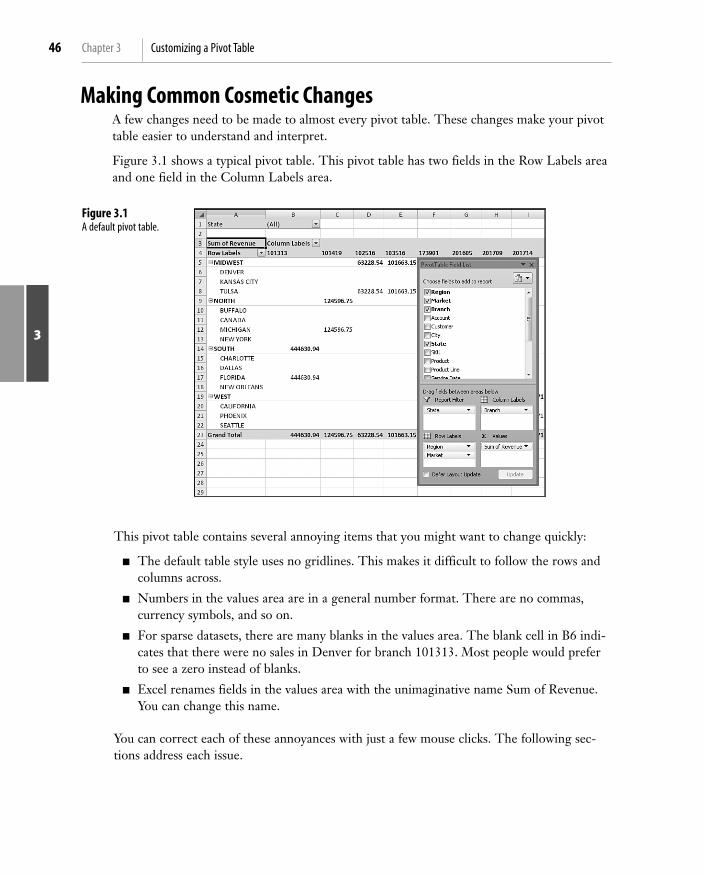
Figure 3.1 shows a typical pivot table. This pivot table has two fields in the Row Labels areaand one field in the Column Labels area.

3

Chapter 3 Customizing a Pivot Table46

Figure 3.1A default pivot table.

This pivot table contains several annoying items that you might want to change quickly:

� The default table style uses no gridlines. This makes it difficult to follow the rows andcolumns across.

� Numbers in the values area are in a general number format. There are no commas,currency symbols, and so on.

� For sparse datasets, there are many blanks in the values area. The blank cell in B6 indi-cates that there were no sales in Denver for branch 101313. Most people would preferto see a zero instead of blanks.

� Excel renames fields in the values area with the unimaginative name Sum of Revenue.You can change this name.

You can correct each of these annoyances with just a few mouse clicks. The following sec-tions address each issue.

CH03.qxd 12/6/06 1:05 PM Page 46

47Making Common Cosmetic Changes

Applying a Table Style to Restore GridlinesThe default pivot table layout contains no gridlines. This format is annoying and a giantstep backward. Luckily, you can easily apply a table style. Any table style that you choosewill be better than the default.

Follow these steps to apply a table style:

1. Make sure that the active cell is in the pivot table.

2. From the Ribbon, choose the Design tab.

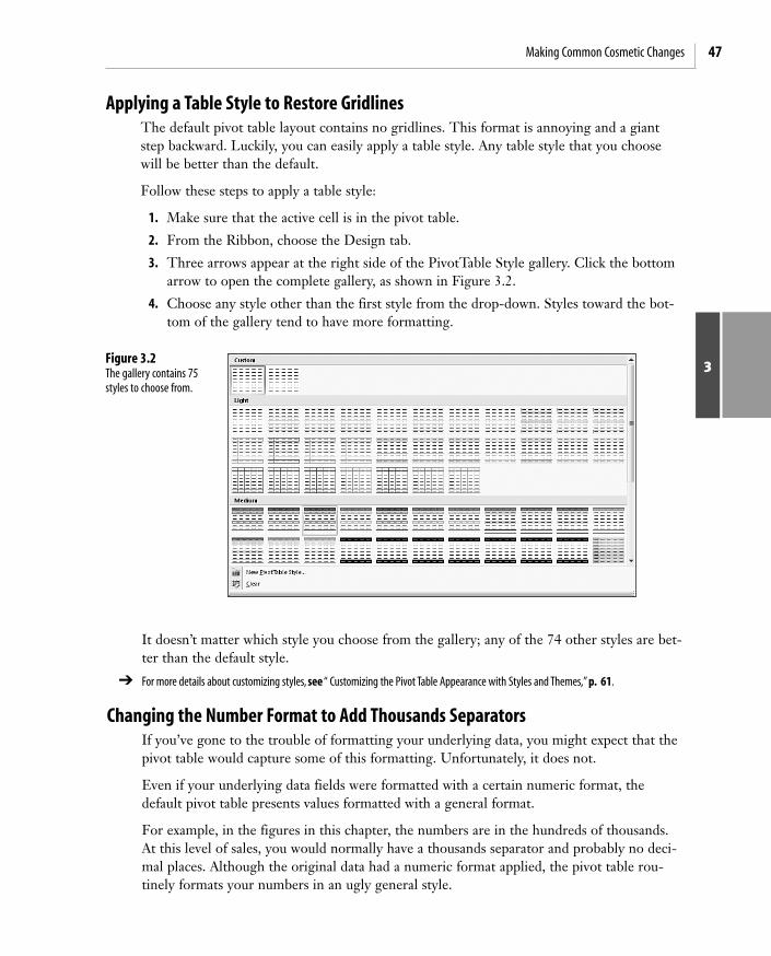
3. Three arrows appear at the right side of the PivotTable Style gallery. Click the bottomarrow to open the complete gallery, as shown in Figure 3.2.

4. Choose any style other than the first style from the drop-down. Styles toward the bot-tom of the gallery tend to have more formatting.

3Figure 3.2The gallery contains 75styles to choose from.

It doesn’t matter which style you choose from the gallery; any of the 74 other styles are bet-ter than the default style.

➔ For more details about customizing styles, see“ Customizing the Pivot Table Appearance with Styles and Themes,” p. 61.

Changing the Number Format to Add Thousands SeparatorsIf you’ve gone to the trouble of formatting your underlying data, you might expect that thepivot table would capture some of this formatting. Unfortunately, it does not.

Even if your underlying data fields were formatted with a certain numeric format, thedefault pivot table presents values formatted with a general format.

For example, in the figures in this chapter, the numbers are in the hundreds of thousands.At this level of sales, you would normally have a thousands separator and probably no deci-mal places. Although the original data had a numeric format applied, the pivot table rou-tinely formats your numbers in an ugly general style.

CH03.qxd 12/6/06 1:05 PM Page 47

You access the numeric format for a field in the Data Field Settings dialog box. There arefour ways to display this dialog box:

� Right-click a number in the values area of the pivot table and choose Value FieldSettings.

� Double-click the Sum of Revenue cell in cell A3 of Figure 3.3.

� Click the drop-down arrow on the Sum of Revenue field in the drop zones of thePivotTable Field List. Then choose Field Settings from the context menu.

� Select any cell in the values area of the pivot table. From the Options ribbon, chooseField Settings from the Active Field group.

As shown in Figure 3.3, the Data Field Settings dialog box is displayed. To change thenumeric format, click the Number Format button in the lower-left corner.

3


Figure 3.3Display the Data FieldSettings dialog box andthen click NumberFormat.

In the Format Cells dialog box, you can choose any built-in number format or choose a cus-tom format. The custom number format shown in Figure 3.4 displays numbers in thousandswith a K abbreviation after the number.

Although Excel 2007 offers a Live Preview feature for many dialog boxes, the Format Cells dialogbox does not offer one.You must assign the number format and then click OK twice to see thechanges.

NO

TE

CH03.qxd 12/6/06 1:05 PM 8


Replacing Blanks with ZerosOne of the elements of good spreadsheet design is that you should never leave blank cells ina numeric section of the worksheet. Even Microsoft believes in this rule; if your source datafor a pivot table contains 1 million numeric cells and 1 blank cell, Excel 2007 treats theentire column as if it were text. This is why it is incredibly annoying that the default settingfor a pivot table leaves many blanks in the values area of some pivot tables.

The blank tells you that there were no sales for that particular combination of labels. In thedefault view, an actual zero is used to indicate that there was activity, but the total sales werezero. This value might mean that a customer bought something and then returned it, result-ing in net sales of zero. Although there are limited applications in which you would want todifferentiate between having no sales and having net zero sales, this seems rare. In 99% ofthe cases, you should fill in the blank cells with zeros.

Follow these steps to change this setting for the current pivot table:

1. Select a cell inside the pivot table.

2. On the Options ribbon, choose the Options icon from the Pivot Table Options groupto display the PivotTable Options dialog box.

3. On the Layout & Format tab, in the Format section, type 0 next to the field labeled ForEmpty Cells Show (see Figure 3.5).

4. Click OK to accept the change.

3

Figure 3.4Choose an easier-to-readnumber format from theFormat Cells dialog box.

CH03.qxd 12/6/06 1:05 PM Page 49

The result is that the pivot table is filled with zeros instead of blanks, as shown in Figure 3.6.

3


Figure 3.5Enter a zero here toreplace the blank cellswith zero.

Enter a zero here

Figure 3.6Your report is now a solidcontiguous block of non-blank cells.

CH03.qxd 12/6/06 1:05 PM Page 50


Changing a Field NameEvery field in the final pivot table has a name. Fields in the row, column, and filter areasinherit their names from the heading in the source data. Fields in the data section are givennames such as Sum of Revenue. In some instances, you may prefer to print a different namein the pivot table. You might prefer Total Revenue instead of the default name. In these situ-ations, the capability to change your field names comes in quite handy.

Although many of the names are inherited from headings in the original dataset, when yourdata is from an external data source, you might not have control over field names. In thesecases, you might want to change the names of the fields as well.

To change a field name in the values area, follow these steps:

1. Select a cell in the pivot table that contains the appropriate value. In Figure 3.7, the val-ues area contains both hours and revenue. If you want to rename Sum of Revenue,select any cell from B5:B24.

2. On the Options ribbon, select the Field Settings icon from the Active Field group.

3. In the Data Field Settings dialog box, type a new name in the Custom Name field. Youcan enter any unique name you like. One common frustration occurs when you wouldlike to rename Sum of Revenue to Revenue. The problem is that this name is notallowed because it is not unique; you already have a Revenue field in the source data. Towork around this limitation, you can name the field and add a space to the end of thename. Excel considers “Revenue” (with a space) to be different from “Revenue” (withno space). Because this change is cosmetic, the readers of your spreadsheet will notnotice the space after the name.

The new name appears in the pivot table. Now look at cell B5 in Figure 3.7. The nameRevenue (with a space) is less awkward than the default Sum of Revenue.

3

Figure 3.7The name typed in theCustom Name boxappears in the pivottable. Although namesshould be unique, youcan trick Excel intoaccepting a similar nameby adding a space to theend of it.

CH03.qxd 12/6/06 1:05 PM Page 51

Making Layout ChangesExcel 2007 offers three layout styles instead of the two styles available in previous versionsof Excel. The new style—Compact Layout—is promoted to be the default layout for yourpivot tables.

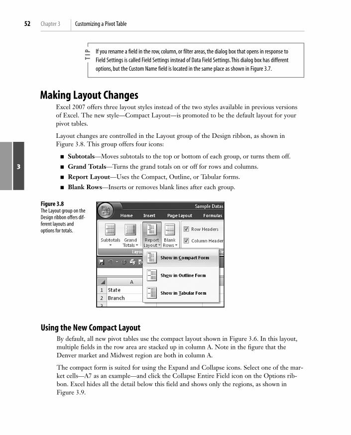
Layout changes are controlled in the Layout group of the Design ribbon, as shown inFigure 3.8. This group offers four icons:

� Subtotals—Moves subtotals to the top or bottom of each group, or turns them off.

� Grand Totals—Turns the grand totals on or off for rows and columns.

� Report Layout—Uses the Compact, Outline, or Tabular forms.

� Blank Rows—Inserts or removes blank lines after each group.

3


If you rename a field in the row, column, or filter areas, the dialog box that opens in response toField Settings is called Field Settings instead of Data Field Settings.This dialog box has differentoptions, but the Custom Name field is located in the same place as shown in Figure 3.7.

TIP

Figure 3.8The Layout group on theDesign ribbon offers dif-ferent layouts andoptions for totals.

Using the New Compact LayoutBy default, all new pivot tables use the compact layout shown in Figure 3.6. In this layout,multiple fields in the row area are stacked up in column A. Note in the figure that theDenver market and Midwest region are both in column A.

The compact form is suited for using the Expand and Collapse icons. Select one of the mar-ket cells—A7 as an example—and click the Collapse Entire Field icon on the Options rib-bon. Excel hides all the detail below this field and shows only the regions, as shown inFigure 3.9.

CH03.qxd 12/6/06 1:05 PM Page 52

53Making Layout Changes

After a field is collapsed, you can show detail for individual regions by using the plus iconsin column A, or you can click Expand Entire Field on the Options ribbon to see the detailagain.

3

Figure 3.9Click the Collapse EntireField icon to hide levelsof detail.

Collapse icon

Plus icon

Figure 3.10When you attempt toexpand the innermostfield, Excel offers to add anew innermost field.

If you select a cell in the innermost row field and click Expand Entire Field, Excel displays the ShowDetail dialog box, as shown in Figure 3.10, to allow you to add a new innermost row field.T

IP

CH03.qxd 12/6/06 1:05 PM Page 53

Using the Outline Form LayoutWhen you select Design, Layout, Report Layout, Show in Outline Form, Excel fills columnA with the outermost row field. Additional row fields occupy columns B, C, and so on.

Figure 3.11 shows the pivot table in Outline form.

3


Figure 3.11The Outline layout putseach row field in a sepa-rate column.

This layout is better suited if you plan to copy the values from the pivot table to a new loca-tion for further analysis. Although the Compact layout offers a clever approach by squeez-ing multiple fields in one column, it is not ideal for reusing the data later.

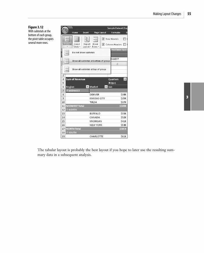
By default, both the Compact and Outline layouts put the subtotals at the top of eachgroup. You can use the Subtotals drop-down on the Design ribbon to move the totals to thebottom of each group, as shown in Figure 3.12.

Using the Traditional Tabular LayoutPivot table veterans will recognize the tabular layout shown in Figure 3.13. This layout issimilar to the one that has been used in pivot tables since their invention. In this layout, thesubtotals can never appear at the top of the group.

CH03.qxd 12/6/06 1:05 PM Page 54

55Making Layout Changes

3

Figure 3.12With subtotals at thebottom of each group,the pivot table occupiesseveral more rows.

The tabular layout is probably the best layout if you hope to later use the resulting sum-mary data in a subsequent analysis.

CH03.qxd 12/6/06 1:05 PM Page 55

C A S E S T U D Y

Converting a Pivot Table to ValuesSay that you want to summarize your dataset to show sales by Region, Market, and Quarter.Your goal is to export this datafor use by another system.

The result in Figure 3.13 is close to the desired output, with a few exceptions:

� The subtotals in rows 9, 14, 19, and 23 should be removed.

� The blank cells in A7:A8, A11:A13, A16:A18, and A21:A22 should be filled in.

� The grand total should be removed from row 24 and column G.

� The pivot table should be converted from a live pivot table to static values.

To make these changes, follow these steps:

1. Select any cell in the pivot table.

2. From the Design ribbon, choose Grand Totals, Off for Rows and Columns.

3


Figure 3.13The tabular layout is sim-ilar to pivot tables inprior versions of Excel.

CH03.qxd 12/6/06 1:05 PM Page 56

57Converting a Pivot Table to Values

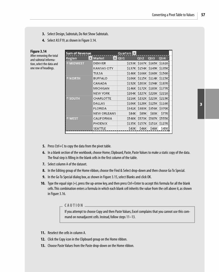
3. Select Design, Subtotals, Do Not Show Subtotals.

4. Select A5:F19, as shown in Figure 3.14.

3

Figure 3.14After removing the totaland subtotal informa-tion, select the data andone row of headings.

5. Press Ctrl+C to copy the data from the pivot table.

6. In a blank section of the workbook, choose Home, Clipboard, Paste, Paste Values to make a static copy of the data.The final step is filling in the blank cells in the first column of the table.

7. Select column A of the dataset.

8. In the Editing group of the Home ribbon, choose the Find & Select drop-down and then choose Go To Special.

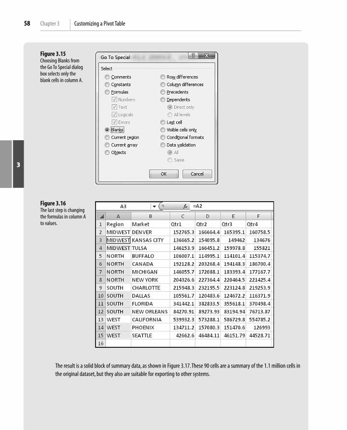
9. In the Go To Special dialog box, as shown in Figure 3.15, select Blanks and click OK.

10. Type the equal sign (=), press the up-arrow key, and then press Ctrl+Enter to accept this formula for all the blankcells.This combination enters a formula in which each blank cell inherits the value from the cell above it, as shownin Figure 3.16.

If you attempt to choose Copy and then Paste Values, Excel complains that you cannot use this com-mand on nonadjacent cells. Instead, follow steps 11–13.

C A U T I O N

11. Reselect the cells in column A.

12. Click the Copy icon in the Clipboard group on the Home ribbon.

13. Choose Paste Values from the Paste drop-down on the Home ribbon.

CH03.qxd 12/6/06 1:05 PM Page 57

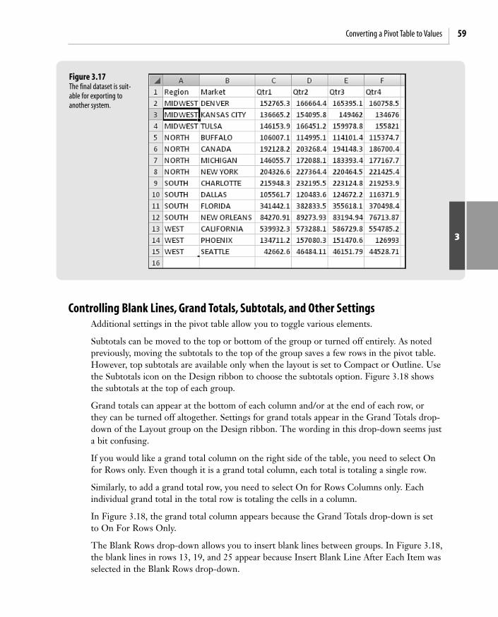
The result is a solid block of summary data, as shown in Figure 3.17.These 90 cells are a summary of the 1.1 million cells inthe original dataset, but they also are suitable for exporting to other systems.

3


Figure 3.15Choosing Blanks fromthe Go To Special dialogbox selects only theblank cells in column A.

Figure 3.16The last step is changingthe formulas in column Ato values.

CH03.qxd 12/6/06 1:05 PM Page 58

59Converting a Pivot Table to Values

Controlling Blank Lines, Grand Totals, Subtotals, and Other SettingsAdditional settings in the pivot table allow you to toggle various elements.

Subtotals can be moved to the top or bottom of the group or turned off entirely. As notedpreviously, moving the subtotals to the top of the group saves a few rows in the pivot table.However, top subtotals are available only when the layout is set to Compact or Outline. Usethe Subtotals icon on the Design ribbon to choose the subtotals option. Figure 3.18 showsthe subtotals at the top of each group.

Grand totals can appear at the bottom of each column and/or at the end of each row, orthey can be turned off altogether. Settings for grand totals appear in the Grand Totals drop-down of the Layout group on the Design ribbon. The wording in this drop-down seems justa bit confusing.

If you would like a grand total column on the right side of the table, you need to select Onfor Rows only. Even though it is a grand total column, each total is totaling a single row.

Similarly, to add a grand total row, you need to select On for Rows Columns only. Eachindividual grand total in the total row is totaling the cells in a column.

In Figure 3.18, the grand total column appears because the Grand Totals drop-down is setto On For Rows Only.

The Blank Rows drop-down allows you to insert blank lines between groups. In Figure 3.18,the blank lines in rows 13, 19, and 25 appear because Insert Blank Line After Each Item wasselected in the Blank Rows drop-down.

3

Figure 3.17The final dataset is suit-able for exporting toanother system.

CH03.qxd 12/6/06 1:05 PM Page 59

As you examine the pivot table in Figure 3.18, you might think the area around B8:B9appears strange. Whereas the sales figures for columns C, D, and E are closely aligned withthe headings, the Qtr1 heading in B8 appears far away from the sales figures in B9:B29.This happens because all the headings in B8:E8 are left-aligned. Something is causing col-umn B to be too wide. That something is the text Column Labels in B7. This text, plus RowLabels in A8, is a new feature in Excel 2007. Although this feature might have beendesigned to improve readability, it is annoying that the text makes column B too wide.

To remove these text entries, click the Field Headers icon in the Show/Hide group on theOptions ribbon. This group also has icons to turn off the plus and minus buttons or to hidethe PivotTable Field List. Figure 3.19 shows this section of the Ribbon, as well as the pivottable with all three items turned off.

3


Figure 3.18Subtotals at the top,grand totals for the rows,and blank lines betweengroups are controlledthrough icons in theLayout group on theDesign ribbon.

Row & ColumnField Headers

CH03.qxd 12/6/06 1:05 PM Page 60

61Customizing the Pivot Table Appearance with Styles and Themes

Customizing the Pivot Table Appearance with Styles and Themes

The PivotTable Styles gallery on the Design ribbon offers 84 built-in styles. Grouped into28 styles each of Light, Medium, and Dark, the gallery offers variations on the accent colorsused in the current theme.

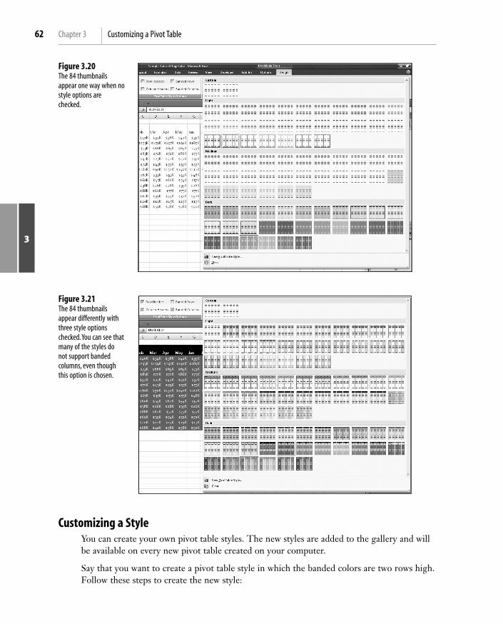
Note that you can modify the thumbnails for the 84 styles shown in the gallery by using thefour check boxes in the PivotTable Style Options group. In Figure 3.20, the 84 styles areshown with all four of the option buttons unchecked.

In Figure 3.21, the 84 styles are shown with accents for row headers, column headers, andalternating colors in the columns.

The PivotTable Style Options group appears to the left of the PivotTable Styles gallery. Ifyou want banded rows or columns, it is best to choose this option before opening thegallery. Some of the 84 themes do not support banded columns or banded rows.

3

Figure 3.19In Excel 2007, field head-ers serve little purpose.

Show/Hide Group

By checking the Banded Columns check box prior to opening the gallery, you can see which stylessupport the banded columns. If the Banded Columns or Rows check box is selected and the thumb-nail in the gallery does not show the effect, you know to avoid that style.

TIP

Excel 2007’s Live Preview feature works in the styles gallery. As you hover your mouse cur-sor over style thumbnails, the worksheet shows a preview of the style.

CH03.qxd 12/6/06 1:05 PM Page 61

3


Figure 3.20The 84 thumbnailsappear one way when nostyle options arechecked.

Figure 3.21The 84 thumbnailsappear differently withthree style optionschecked.You can see thatmany of the styles donot support bandedcolumns, even thoughthis option is chosen.

Customizing a StyleYou can create your own pivot table styles. The new styles are added to the gallery and willbe available on every new pivot table created on your computer.

Say that you want to create a pivot table style in which the banded colors are two rows high.Follow these steps to create the new style:

CH03.qxd 12/6/06 1:05 PM Page 62

63Customizing the Pivot Table Appearance with Styles and Themes

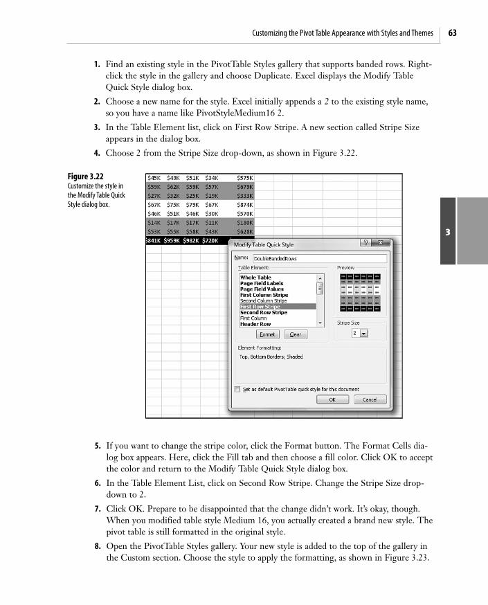
1. Find an existing style in the PivotTable Styles gallery that supports banded rows. Right-click the style in the gallery and choose Duplicate. Excel displays the Modify TableQuick Style dialog box.

2. Choose a new name for the style. Excel initially appends a 2 to the existing style name,so you have a name like PivotStyleMedium16 2.

3. In the Table Element list, click on First Row Stripe. A new section called Stripe Sizeappears in the dialog box.

4. Choose 2 from the Stripe Size drop-down, as shown in Figure 3.22.

3

Figure 3.22Customize the style inthe Modify Table QuickStyle dialog box.

5. If you want to change the stripe color, click the Format button. The Format Cells dia-log box appears. Here, click the Fill tab and then choose a fill color. Click OK to acceptthe color and return to the Modify Table Quick Style dialog box.

6. In the Table Element List, click on Second Row Stripe. Change the Stripe Size drop-down to 2.

7. Click OK. Prepare to be disappointed that the change didn’t work. It’s okay, though.When you modified table style Medium 16, you actually created a brand new style. Thepivot table is still formatted in the original style.

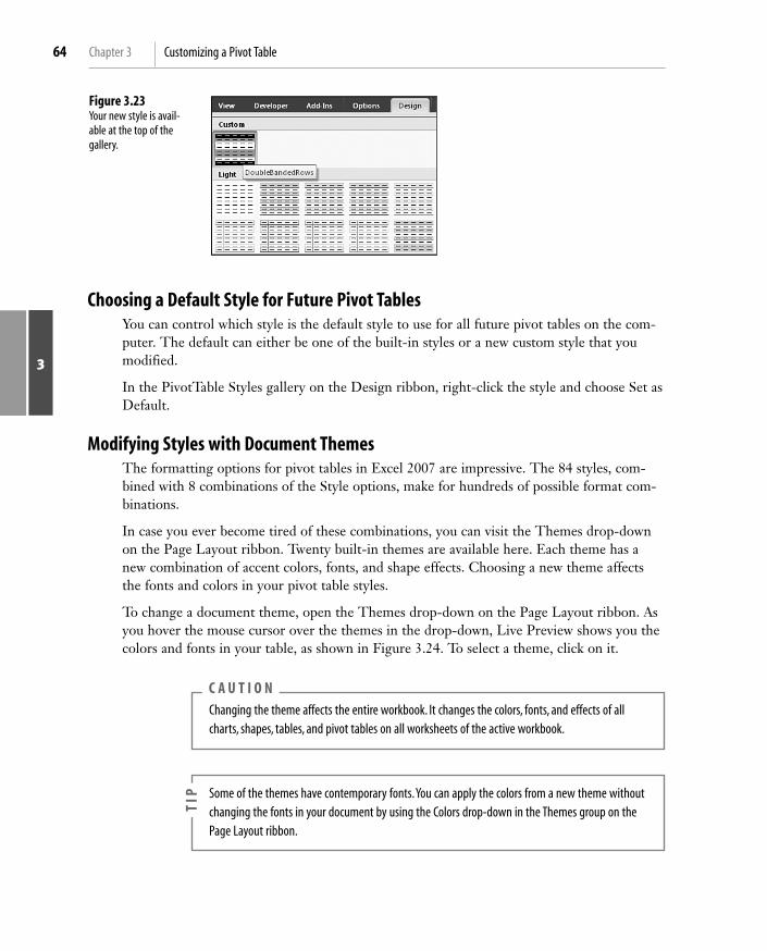
8. Open the PivotTable Styles gallery. Your new style is added to the top of the gallery inthe Custom section. Choose the style to apply the formatting, as shown in Figure 3.23.

CH03.qxd 12/6/06 1:05 PM Page 63

Choosing a Default Style for Future Pivot TablesYou can control which style is the default style to use for all future pivot tables on the com-puter. The default can either be one of the built-in styles or a new custom style that youmodified.

In the PivotTable Styles gallery on the Design ribbon, right-click the style and choose Set asDefault.

Modifying Styles with Document ThemesThe formatting options for pivot tables in Excel 2007 are impressive. The 84 styles, com-bined with 8 combinations of the Style options, make for hundreds of possible format com-binations.

In case you ever become tired of these combinations, you can visit the Themes drop-downon the Page Layout ribbon. Twenty built-in themes are available here. Each theme has anew combination of accent colors, fonts, and shape effects. Choosing a new theme affectsthe fonts and colors in your pivot table styles.

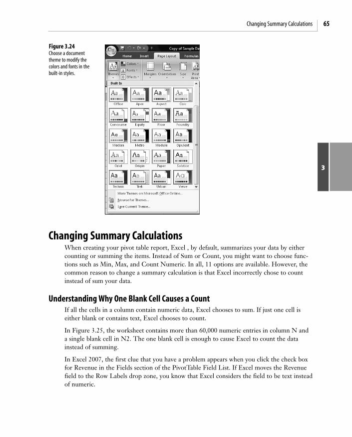
To change a document theme, open the Themes drop-down on the Page Layout ribbon. Asyou hover the mouse cursor over the themes in the drop-down, Live Preview shows you thecolors and fonts in your table, as shown in Figure 3.24. To select a theme, click on it.

3


Figure 3.23Your new style is avail-able at the top of thegallery.

Changing the theme affects the entire workbook. It changes the colors, fonts, and effects of allcharts, shapes, tables, and pivot tables on all worksheets of the active workbook.

C A U T I O N

Some of the themes have contemporary fonts.You can apply the colors from a new theme withoutchanging the fonts in your document by using the Colors drop-down in the Themes group on thePage Layout ribbon.

TIP

CH03.qxd 12/6/06 1:05 PM Page 64

65Changing Summary Calculations

Changing Summary CalculationsWhen creating your pivot table report, Excel , by default, summarizes your data by eithercounting or summing the items. Instead of Sum or Count, you might want to choose func-tions such as Min, Max, and Count Numeric. In all, 11 options are available. However, thecommon reason to change a summary calculation is that Excel incorrectly chose to countinstead of sum your data.

Understanding Why One Blank Cell Causes a CountIf all the cells in a column contain numeric data, Excel chooses to sum. If just one cell iseither blank or contains text, Excel chooses to count.

In Figure 3.25, the worksheet contains more than 60,000 numeric entries in column N anda single blank cell in N2. The one blank cell is enough to cause Excel to count the datainstead of summing.

In Excel 2007, the first clue that you have a problem appears when you click the check boxfor Revenue in the Fields section of the PivotTable Field List. If Excel moves the Revenuefield to the Row Labels drop zone, you know that Excel considers the field to be text insteadof numeric.

3

Figure 3.24Choose a documenttheme to modify thecolors and fonts in thebuilt-in styles.

CH03.qxd 12/6/06 1:05 PM Page 65

Be vigilant while dragging fields into the Values drop zone. If a calculation appears to bedramatically too low, check to see whether the field name reads Count of Revenue instead ofSum of Revenue. When you created the pivot table in Figure 3.26, you should have noticedthat your company had only $68,613 in revenue instead of $10 million. This should be ahint to notice that the heading in B3 reads Count of Revenue instead of Sum of Revenue. Infact, 68,613 is the number of records in the dataset.

3


Figure 3.25The single blank cell inN2 causes problems inthe default pivot table.

Figure 3.26Your revenue numberslook anemic. Notice incell B3 that Excel choseto count instead of sumthe revenue.This oftenhappens if you inadver-tently have one blankcell in your Revenue column.

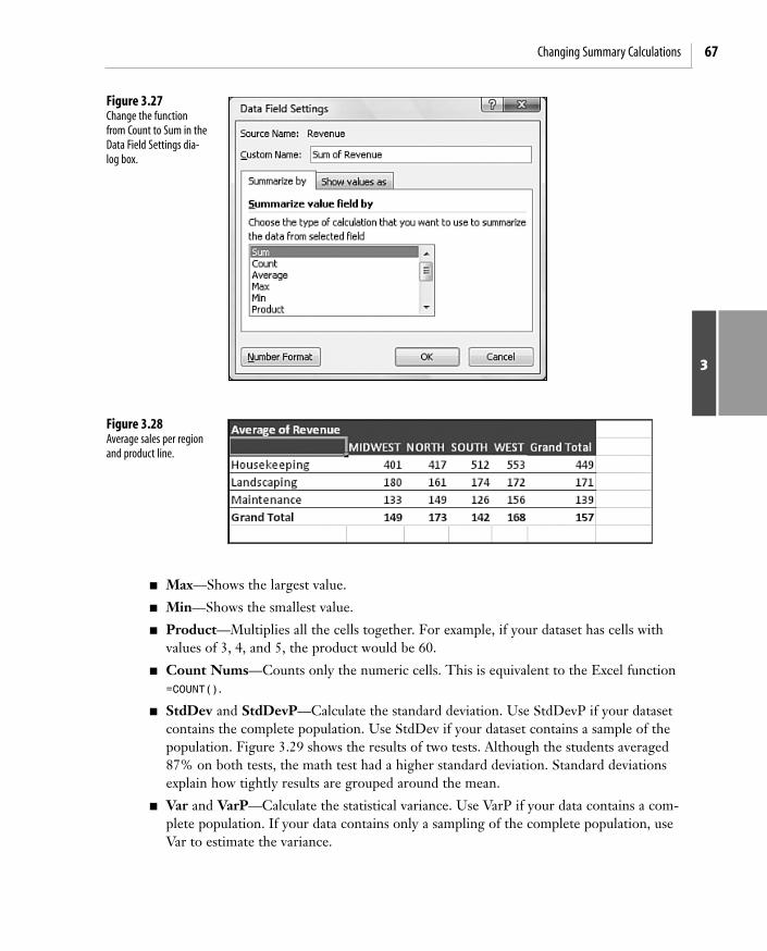
You can easily override the incorrect Count calculation. Activate the Data Field Settingsdialog box by double-clicking on Count of Revenue and then change the Summarize ValueField By setting from Count to Sum, as shown in Figure 3.27.

Using Functions Other Than Count or SumExcel offers a total of 11 functions in the Summarize By section of the PivotTable Field dia-log box. The options available are as follows:

� Sum—Provides a total of all numeric data.

� Count—Counts all cells, including numeric, text, and error cells. This is equivalent tothe Excel function =COUNTA().

� Average—Provides an average. Figure 3.28 shows a report detailing average sales perregion and product line. An analyst might wonder why the average housekeeping salein the West is $152 higher than in the Midwest.

CH03.qxd 12/6/06 1:05 PM Page 66

67Changing Summary Calculations

� Max—Shows the largest value.

� Min—Shows the smallest value.

� Product—Multiplies all the cells together. For example, if your dataset has cells withvalues of 3, 4, and 5, the product would be 60.

� Count Nums—Counts only the numeric cells. This is equivalent to the Excel function=COUNT().

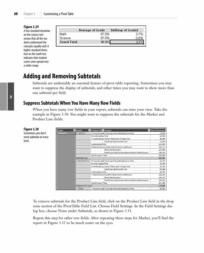
� StdDev and StdDevP—Calculate the standard deviation. Use StdDevP if your datasetcontains the complete population. Use StdDev if your dataset contains a sample of thepopulation. Figure 3.29 shows the results of two tests. Although the students averaged87% on both tests, the math test had a higher standard deviation. Standard deviationsexplain how tightly results are grouped around the mean.

� Var and VarP—Calculate the statistical variance. Use VarP if your data contains a com-plete population. If your data contains only a sampling of the complete population, useVar to estimate the variance.

3

Figure 3.27Change the functionfrom Count to Sum in theData Field Settings dia-log box.

Figure 3.28Average sales per regionand product line.

CH03.qxd 12/6/06 1:05 PM Page 67

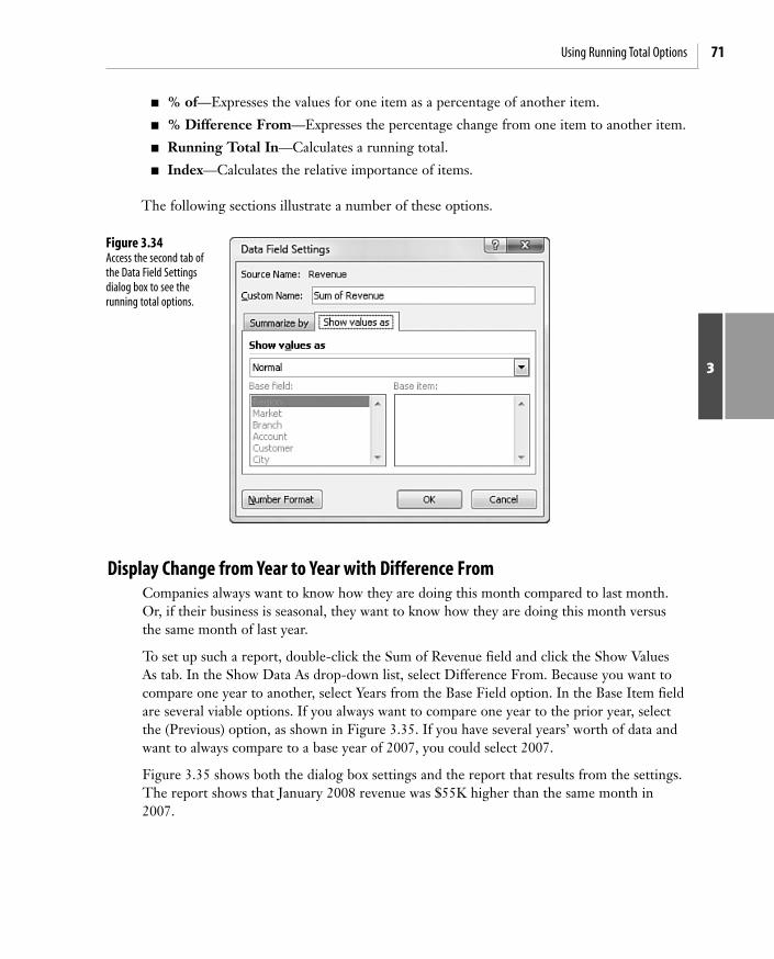
Adding and Removing SubtotalsSubtotals are undeniably an essential feature of pivot table reporting. Sometimes you maywant to suppress the display of subtotals, and other times you may want to show more thanone subtotal per field.

Suppress Subtotals When You Have Many Row FieldsWhen you have many row fields in your report, subtotals can mire your view. Take theexample in Figure 3.30. You might want to suppress the subtotals for the Market andProduct Line fields.

3


Figure 3.29A low standard deviationon the science testmeans that all the stu-dents understand theconcepts equally well. Ahigher standard devia-tion on the math testindicates that studentscores were spread overa wider range.

Figure 3.30Sometimes you don’tneed subtotals at everylevel.

To remove subtotals for the Product Line field, click on the Product Line field in the dropzone section of the PivotTable Field List. Choose Field Settings. In the Field Settings dia-log box, choose None under Subtotals, as shown in Figure 3.31.

Repeat this step for other row fields. After repeating these steps for Market, you’ll find thereport in Figure 3.32 to be much easier on the eyes.

CH03.qxd 12/6/06 1:05 PM Page 68

69Adding and Removing Subtotals

Adding Multiple Subtotals for One FieldYou can add customized subtotals to a row or column label field. Select the Region field inthe drop zone of the PivotTable Field List and choose Field Settings.

3

Figure 3.31Choose None to removesubtotals at the ProductLine level.

Figure 3.32After specifying None fortwo fields, you give thereport a cleaner look.

If you want to suppress the subtotals for all the row fields, it is easier to choose Design, Layout,Subtotals, Do Not Show Subtotals.T

IP

CH03.qxd 12/6/06 1:05 PM Page 69

In the Field Settings dialog box, choose Custom and select the types of subtotals you wouldlike to see. The dialog box in Figure 3.33 shows five subtotals selected for the Region field.

3


Figure 3.33By selecting the Customoption in the Subtotalssection, you can specifymultiple subtotals forone field.

Using Running Total OptionsSo far, every pivot table created has used the Normal option. When you want to create run-ning totals or compare an item to another item, you have eight choices other than Normal.

The nine options are on the second tab of the Data Field Settings dialog box. To accessthem, follow these steps:

1. Select a cell in the values area of your pivot table. Or, select the Sum of Revenue cell.

2. On the Options ribbon, click the Field Settings icon in the Active Group field.

3. Click the Show Values As tab in the Data Field Settings dialog box.

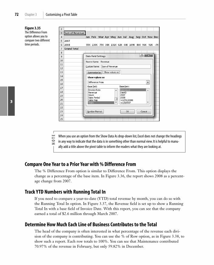
Initially, the Show Values As drop-down is set to Normal, and the Base Field and Base Itemlist boxes are grayed out, as shown in Figure 3.34.

The capability to create custom calculations is another example of the unique flexibility ofpivot table reports. With the Show Data As setting, you can change the calculation for aparticular data field to be based on other cells in the values area.

When you click the Show Values As drop-down, you have eight choices other than Normal.The choices are

� % of Row—Shows percentages that total across the pivot table to 100%.

� % of Column—Shows percentages that total up and down the pivot table to 100%.

� % of Total—Shows percentages such that all the detail cells in the pivot table total to100%.

� Difference From—Shows the difference of one item compared to another item or tothe previous item.

CH03.qxd 12/6/06 1:05 PM Page 70

71Using Running Total Options

� % of—Expresses the values for one item as a percentage of another item.

� % Difference From—Expresses the percentage change from one item to another item.

� Running Total In—Calculates a running total.

� Index—Calculates the relative importance of items.

The following sections illustrate a number of these options.

3

Figure 3.34Access the second tab ofthe Data Field Settingsdialog box to see therunning total options.

Display Change from Year to Year with Difference FromCompanies always want to know how they are doing this month compared to last month.Or, if their business is seasonal, they want to know how they are doing this month versusthe same month of last year.

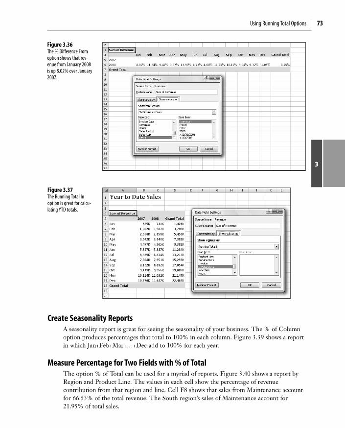
To set up such a report, double-click the Sum of Revenue field and click the Show ValuesAs tab. In the Show Data As drop-down list, select Difference From. Because you want tocompare one year to another, select Years from the Base Field option. In the Base Item fieldare several viable options. If you always want to compare one year to the prior year, selectthe (Previous) option, as shown in Figure 3.35. If you have several years’ worth of data andwant to always compare to a base year of 2007, you could select 2007.

Figure 3.35 shows both the dialog box settings and the report that results from the settings.The report shows that January 2008 revenue was $55K higher than the same month in2007.

CH03.qxd 12/6/06 1:05 PM Page 71

3


Figure 3.35The Difference Fromoption allows you tocompare two differenttime periods.

Compare One Year to a Prior Year with % Difference FromThe % Difference From option is similar to Difference From. This option displays thechange as a percentage of the base item. In Figure 3.36, the report shows 2008 as a percent-age change from 2007.

Track YTD Numbers with Running Total InIf you need to compare a year-to-date (YTD) total revenue by month, you can do so withthe Running Total In option. In Figure 3.37, the Revenue field is set up to show a RunningTotal In with a base field of Invoice Date. With this report, you can see that the companyearned a total of $2.6 million through March 2007.

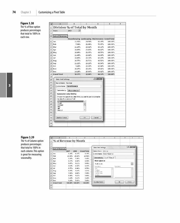
Determine How Much Each Line of Business Contributes to the TotalThe head of the company is often interested in what percentage of the revenue each divi-sion of the company is contributing. You can use the % of Row option, as in Figure 3.38, toshow such a report. Each row totals to 100%. You can see that Maintenance contributed70.97% of the revenue in February, but only 59.82% in December.

When you use an option from the Show Data As drop-down list, Excel does not change the headingsin any way to indicate that the data is in something other than normal view. It is helpful to manu-ally add a title above the pivot table to inform the readers what they are looking at.

NO

TE

CH03.qxd 12/6/06 1:05 PM Page 72


Create Seasonality ReportsA seasonality report is great for seeing the seasonality of your business. The % of Columnoption produces percentages that total to 100% in each column. Figure 3.39 shows a reportin which Jan+Feb+Mar+…+Dec add to 100% for each year.

Measure Percentage for Two Fields with % of TotalThe option % of Total can be used for a myriad of reports. Figure 3.40 shows a report byRegion and Product Line. The values in each cell show the percentage of revenue contribution from that region and line. Cell F8 shows that sales from Maintenance accountfor 66.53% of the total revenue. The South region’s sales of Maintenance account for21.95% of total sales.

3

Figure 3.36The % Difference Fromoption shows that rev-enue from January 2008is up 8.02% over January2007.

Figure 3.37The Running Total Inoption is great for calcu-lating YTD totals.

CH03.qxd 12/6/06 1:05 PM Page 73

3


Figure 3.38The % of Row optionproduces percentagesthat total to 100% ineach row.

Figure 3.39The % of Column optionproduces percentagesthat total to 100% ineach column.This optionis great for measuringseasonality.

CH03.qxd 12/6/06 1:05 PM Page 74


3

Figure 3.40The % of Total optionproduces a report inwhich every cell is a per-centage of total sales.The manager of theSouth RegionMaintenance depart-ment can use this reportto explain why hisdepartment should get araise this year.

Compare One Line to Another Line Using % OfThe % Of option allows you to compare one item to another item. This comparison mightbe relevant if you believe that housekeeping and landscaping should be related. You can setup a pivot table that compares each product line to landscaping revenue. The result isshown in Figure 3.41.

Track Relative Importance with the Index OptionThe final option, Index, creates a fairly obscure calculation. Microsoft claims that this calcu-lation describes the relative importance of a cell within a column.

Look at the normal data at the top of Figure 3.42. To calculate the index for GeorgiaPeaches, Excel first calculates Georgia Peaches x Grand Total Sales. This would be $180 x$848. Next, Excel calculates Georgia Sales x Peach Sales. This would be $210 x $290. Itthen divides the first result by the second result to come up with a relative importance indexof 2.51.

CH03.qxd 12/6/06 1:05 PM Page 75

3


Figure 3.41This report is createdusing the % Of optionwith Landscaping as thebase item.

Figure 3.42Using the Index function,Excel shows that peachsales are more importantin Georgia than inTennessee.

CH03.qxd 12/6/06 1:05 PM Page 76

C A S E S T U D Y

77Producing Revenue by Line of Business Report

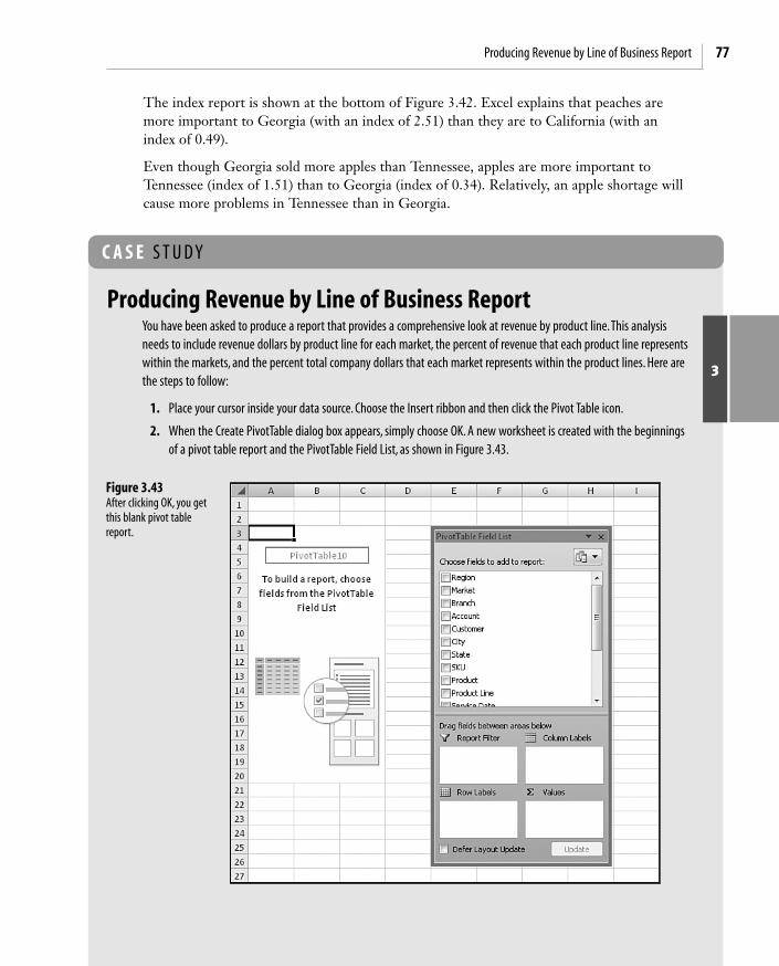
Producing Revenue by Line of Business ReportYou have been asked to produce a report that provides a comprehensive look at revenue by product line.This analysisneeds to include revenue dollars by product line for each market, the percent of revenue that each product line representswithin the markets, and the percent total company dollars that each market represents within the product lines. Here arethe steps to follow:

1. Place your cursor inside your data source. Choose the Insert ribbon and then click the Pivot Table icon.

2. When the Create PivotTable dialog box appears, simply choose OK. A new worksheet is created with the beginningsof a pivot table report and the PivotTable Field List, as shown in Figure 3.43.

3

The index report is shown at the bottom of Figure 3.42. Excel explains that peaches aremore important to Georgia (with an index of 2.51) than they are to California (with anindex of 0.49).

Even though Georgia sold more apples than Tennessee, apples are more important toTennessee (index of 1.51) than to Georgia (index of 0.34). Relatively, an apple shortage willcause more problems in Tennessee than in Georgia.

Figure 3.43After clicking OK, you getthis blank pivot tablereport.

CH03.qxd 12/6/06 1:05 PM Page 77

3


Figure 3.44Setting up the row andcolumn fields.

Figure 3.45Having three copies ofSum of Revenue doesn’tlook useful…yet.

3. Click the Market field in the fields section of the PivotTable Field List to automatically move Market to the RowLabels drop zone.Then drag the Product Line field into the Column Labels drop zone, as shown in Figure 3.44.

4. Drag the Revenue field into the Values drop zone three times to create three separate revenue data items.There is a new Sum Values item in the Column Labels drop zone. Move this to the Row Labels drop zone, as shown inFigure 3.45.

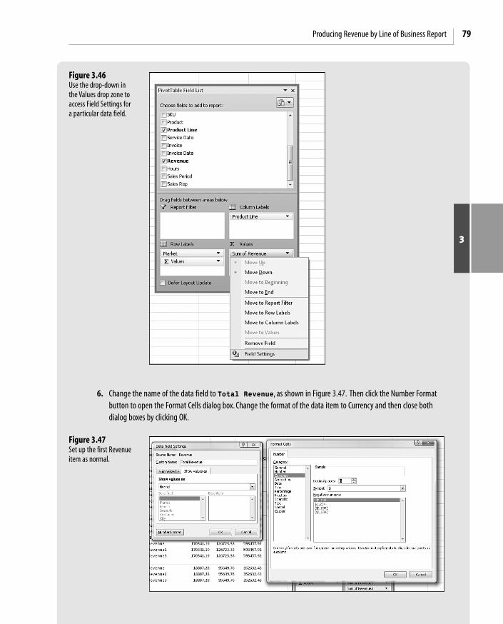
5. In the Values drop zone, click on the first Sum of Revenue field and select Field Settings, as shown in Figure 3.46.

CH03.qxd 12/6/06 1:05 PM Page 78

79Producing Revenue by Line of Business Report

3

Figure 3.46Use the drop-down inthe Values drop zone toaccess Field Settings fora particular data field.

6. Change the name of the data field to Total Revenue, as shown in Figure 3.47. Then click the Number Formatbutton to open the Format Cells dialog box. Change the format of the data item to Currency and then close both dialog boxes by clicking OK.

Figure 3.47Set up the first Revenueitem as normal.

CH03.qxd 12/6/06 1:05 PM Page 79

7. Open the Data Field Settings for the Sum of Revenue2 field.

8. Change the name of the data field to Percent of Market. On the Show Values As tab, in the Show Values Asdrop-down, select the % of Row option. After you do that, choose the Number Format button to open the FormatCells dialog box. Change the format of the cells to Percentage, as shown in Figure 3.48. Close both dialog boxes byclicking OK twice.

3


Figure 3.48Use % of Row to get thePercentage of Market.

9. Open the Date Field Settings dialog box for Sum of Revenue3.

10. Change the name of the data field to Percent of Company. On the Show Values As tab, choose the % ofColumn option. After you do that, choose the Number button to open the Format Cells dialog box. Change the for-mat of the cells to Percentage and then close both dialog boxes by clicking OK.

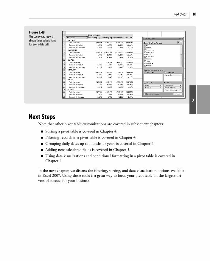
As shown in Figure 3.49, your product line analysis is complete! You have the Total Revenue field, which gives you the rev-enue dollars by product line for each market.Then you have the Percent of Market field, which shows you the percent ofrevenue that each line represents within the markets. Finally, you have the Percent of Company field, which shows line ofbusiness revenue as a percentage of total company dollars.

CH03.qxd 12/6/06 1:05 PM Page 80

81Next Steps

Next StepsNote that other pivot table customizations are covered in subsequent chapters:

� Sorting a pivot table is covered in Chapter 4.

� Filtering records in a pivot table is covered in Chapter 4.

� Grouping daily dates up to months or years is covered in Chapter 4.

� Adding new calculated fields is covered in Chapter 5.

� Using data visualizations and conditional formatting in a pivot table is covered inChapter 4.

In the next chapter, we discuss the filtering, sorting, and data visualization options availablein Excel 2007. Using these tools is a great way to focus your pivot table on the largest dri-vers of success for your business.

3

Figure 3.49The completed reportshows three calculationsfor every data cell.

CH03.qxd 12/6/06 1:05 PM Page 81

CH03.qxd 12/6/06 1:05 PM Page 82

ch03.qxd 12/6/06 1:05 pm page 45 customizing a pivot table...

Documents