ch02 discrete systems
DESCRIPTION
FEATRANSCRIPT

Analysis of
Discrete Systems
Jayadeep U. B.
M.E.D., NIT Calicut

2
Department of Mechanical Engineering, National Institute of Technology Calicut
Introduction
The systems, which can be considered as an assembly of discrete elements, like trusses, electrical resistance networks, assembly of springs etc., are called discrete systems.
Discrete systems depends on finite number of parameters, like the displacements and forces at the joints in a truss, as against a continuous variation of displacement in a continuous system.
From analysis perspective, the significant difference between a discrete system and a continuous system is that the behavior of discrete systems is governed by algebraic equations connecting the system parameters, while continuous systems lead to differential equations.
Lecture - 01
What are Discrete Systems?
FEM is a method for continuous systems. However, the fundamental idea is to convert the D.E. to algebraic equations – Hence, we will learn the discrete system analysis first.

3
Department of Mechanical Engineering, National Institute of Technology Calicut
First 1D Example – Assembly of Springs
The elements of a discrete system are directly obvious – Springs 1 & 2 above.
A set of discrete parameters (called System Variables) can be easily identified – the nodal displacements here.
F3
k(2)k(1)
1 21 2 3
Using the equation for springs in series:
3 (1) (2)
(1) (2)
(1) (2)
F F Fu
k k K
k kK
k k
Lecture - 01

4
Department of Mechanical Engineering, National Institute of Technology Calicut
1D Examples contd. …
Considering a general element (e), with nodes “i” & “j” and nodal displacements & forces as shown below:
Note: The directions shown are for the forces on the element by the nodes… force on the nodes by the element will have opposite sign.
Therefore, we have:
( ) ( )
( ) ( )
( ) ( ) ( )
( )
( ) ( )
e ei j
e ei i j
e e ej j i i j
f f
f k u u
f k u u k u u
k(e)
ei jfi(e)
uiuj
fj(e)
Lecture - 01
5
Department of Mechanical Engineering, National Institute of Technology Calicut
1D Examples contd. …
( ) ( ) ( )
( ) ( )( )
e e ei i
e eejj
f uk kuk kf
(1) (1) (1)1 1
(1) (1)(1)22
f uk k
uk kf
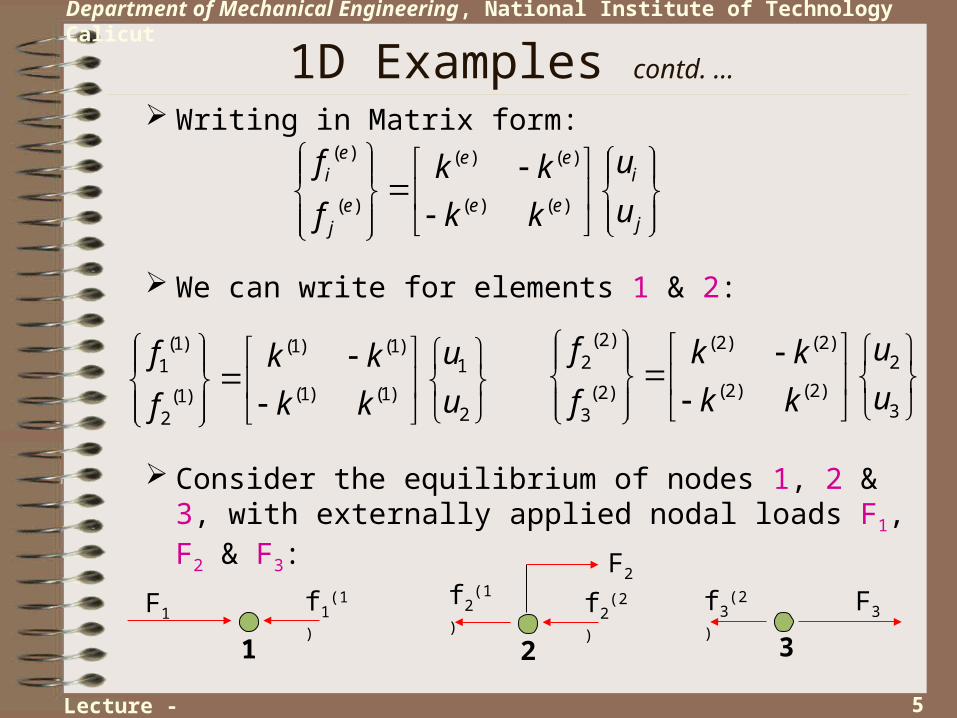
Writing in Matrix form:
We can write for elements 1 & 2:
Consider the equilibrium of nodes 1, 2 & 3, with externally applied nodal loads F1, F2 & F3:
(2) (2) (2)2 2
(2) (2)(2)33
f uk k
uk kf
f1(1)F1
1
f2(2)
F2
f2(1)
2
f3(2) F3
3
Lecture - 01
6
Department of Mechanical Engineering, National Institute of Technology Calicut
1D Example contd. …
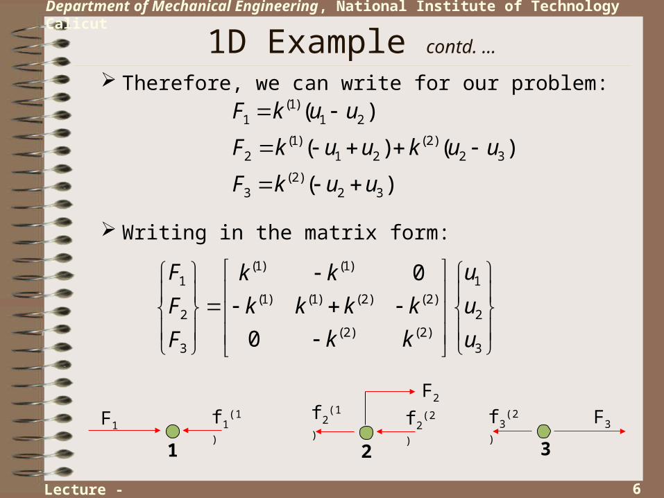
(1)1 1 2
(1) (2)2 1 2 2 3
(2)3 2 3
( )
( ) ( )
( )
F k u u
F k u u k u u
F k u u
(1) (1)1 1
(1) (1) (2) (2)2 2
(2) (2)3 3
0
0
F uk k
F k k k k u
k kF u
Therefore, we can write for our problem:
Writing in the matrix form:
f1(1)F1
1
f2(2)
F2
f2(1)
2
f3(2) F3
3
Lecture - 01
7
Department of Mechanical Engineering, National Institute of Technology Calicut
1D Examples contd. …
(1) (1)1 1
(1) (1) (2) (2)2 2
(2) (2)3 3
0
0
{ } { }
u Fk k
k k k k u F
k k u F
K u f
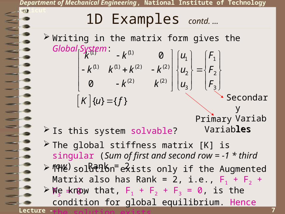
Writing in the matrix form gives the Global System:
Is this system solvable?Primary Variables
Secondary Variables
The global stiffness matrix [K] is singular (Sum of first and second row = -1 * third row) . Rank = 2.
The solution exists only if the Augmented Matrix also has Rank = 2, i.e., F1 + F2 + F3 = 0.
We know that, F1 + F2 + F3 = 0, is the condition for global equilibrium. Hence the solution exists.
Lecture - 01
8
Department of Mechanical Engineering, National Institute of Technology Calicut
1D Examples contd. …
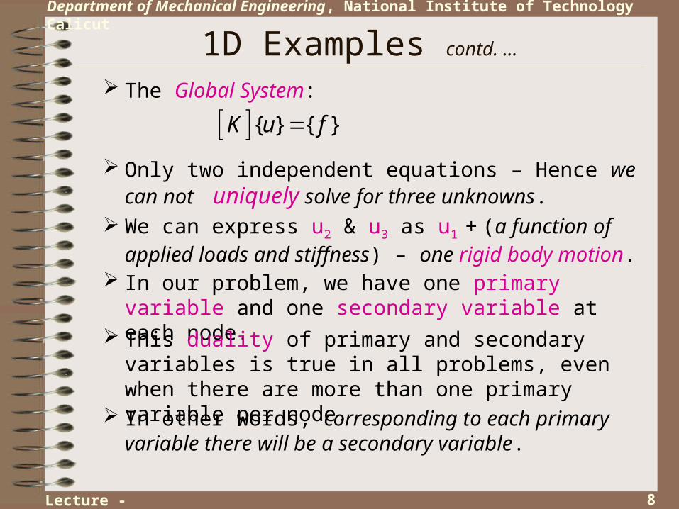
{ } { }K u f
The Global System:
Only two independent equations – Hence we can not uniquely solve for three unknowns.
We can express u2 & u3 as u1 + (a function of applied loads and stiffness) – one rigid body motion.
In our problem, we have one primary variable and one secondary variable at each node.
This duality of primary and secondary variables is true in all problems, even when there are more than one primary variable per node.
In other words, corresponding to each primary variable there will be a secondary variable.
Lecture - 01

9
Department of Mechanical Engineering, National Institute of Technology Calicut
1D Examples contd. …
(1) (1)1 1
(1) (1) (2) (2)2 2
(2) (2)3 3 3
0 ?0
? 0
0 ?
u Fk k
k k k k u F
k k u F F
Applying the Boundary conditions (B.C.):
To solve the system, we can use the last two equations:
(1) (2) (2)2 3
(2) (2)2 3 3
( ) 0k k u k u
k u k u F
On solving, we get:
(1) 3(1)2 3 2
(1) (2)(2) 3
(1)3 3 3 3(2) (1) (2)
1
Fk u F uk
k kFu F k u Fkk k k
Lecture - 01
10
Department of Mechanical Engineering, National Institute of Technology Calicut
1D Examples contd. …
(1)(1)1 11
(1) (2) (2) (1)2 2 1
(2) (2)3 3 1
0 0
0
0 0
F k uuk
k k k u F k u
k k u F u
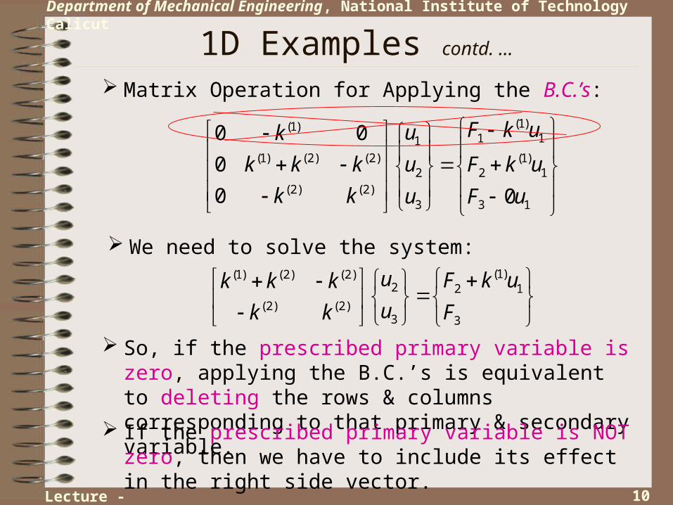
Matrix Operation for Applying the B.C.’s:
We need to solve the system:(1)(1) (2) (2)
2 2 1
(2) (2)3 3
u F k uk k k
u Fk k
So, if the prescribed primary variable is zero, applying the B.C.’s is equivalent to deleting the rows & columns corresponding to that primary & secondary variable.
If the prescribed primary variable is NOT zero, then we have to include its effect in the right side vector.
Lecture - 01

11
Department of Mechanical Engineering, National Institute of Technology Calicut
1D Examples contd. …
Other examples of Discrete 1D systems: 1) Electrical resistance networks
Primary variables: Voltages at Junctions
2) Piping (Fluid Flow) Networks
3) 1D Structural Systems (Springs, Links, columns with steps …)
Secondary variables: Currents
Elements: Resistances
Governing Equations: Ohms Law, Kirchhoff’s Laws
Primary variables: Heads at junctions Secondary variables: Flow rates
Elements: Pipes or Conduits
Governing Equations: Laminar or Turbulent flow relations
Lecture - 01

12
Department of Mechanical Engineering, National Institute of Technology Calicut
Spring System again!!!:
Considering a general element (e) with nodes i & j:
( )( ) ( )
( )( ) ( )
ee ei i
ee ej j
u fk ku fk k
F1
21
2
3
34
Elemental Stiffness- Matrix
Elemental - Displacement Vector
Elemental Force Vector
Second 1D Example
Lecture - 02

13
Department of Mechanical Engineering, National Institute of Technology Calicut
Writing in a general form:
( ) ( ) ( )
( ) ( ) ( )
e e eiii ij i
e e ejji jj j
uk k f
uk k f
1D Examples contd. …
In our case:( ) ( ) ( )
( ) ( ) ( )
&e e eii jj
e e eij ji
k k k
k k k
What does kij(e) mean?
( ) ( ) ( ) ( )
( ) ( ) ( ) ( )
0
1
e e e eii ij i ij
e e e eji jj j jj
k k f k
k k f k
Lecture - 02

14
Department of Mechanical Engineering, National Institute of Technology Calicut
Consider element 1:
(1) (1) (1)111 13 1
(1) (1) (1)331 33 3
uk k f
uk k f
1D Examples contd. …
Contribution of element 1 to the Global System:(1) (1)
11 13 1 1
2 2(1) (1)
31 33 3 3
0
0 0 0
0
k k u F
u F
k k u F
Add the contribution from element 2.
(1) (1)11 13 1 1
2 2(1) (1)
31 33
(2
3
) (2)11 12
(2) (2)21
3
22 0
0
k k
k
k k u F
u F
k k u F
k
Lecture - 02

15
Department of Mechanical Engineering, National Institute of Technology Calicut
1D Examples contd. …
Add the contribution from element 3.
(3) (3)11 12
(3) (3)21 22
(1) (2) (2) (1)11 11 12 13 1 1
(2) (2)21 22 2 2
(1) (1)31 33 3 3
0
0
k k k k u F
k k u F
k k
k
k u F
k
k
Add the contribution from element 4.
(4) (4)22 2
(1) (2) (3) (2) (3) (1)1
3(4
1 11 11 12 12 13 1 1(2) (3) (2) (3)
21 21 22 22 2 2(1) (1)
31) (4)
32 3333 3 3
k k k k k k u F
k k k k u F
k k u F
k k
k k
Global Stiffness Matrix Global Displacement -Vector
Global Force Vector
What does a 0 in the Global Stiffness Matrix mean?
Lecture - 02

16
Department of Mechanical Engineering, National Institute of Technology Calicut
1D Examples contd. … In our specific problem: Study the Stiffness matrix
(1) (2) (3) (2) (3) (1)1 1
(2) (3) (2) (3) (4) (4)2 2
(1) (4) (1) (4)3 3
k k k k k k u F
k k k k k k u F
k k k k u F
Symmetric Matrix. Sum of the elements in every row equals to zero. This implies
rigid body motion. Hence, it is true only if unit (or constant) value for displacements in the global displacement vector causes a rigid body motion.
Sum of the elements in every column equals to zero. This implies equilibrium of a node. Note: This case corresponds to unit displacement applied to one node and hence, the forces developed external to the body should be in equilibrium.
Another important property of stiffness matrix in FEM is the Sparse nature – It is not obvious in this small system.
Lecture - 02
17
Department of Mechanical Engineering, National Institute of Technology Calicut
1D Examples contd. …
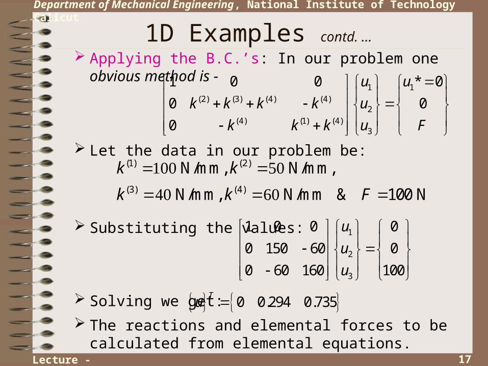
Applying the B.C.’s: In our problem one obvious method is -
1 1(2) (3) (4) (4)
2(4) (1) (4)
3
1 0 0 * 0
0 0
0
u u
k k k k u
k k k u F
Let the data in our problem be:(1) (2)
(3) (4)
Ν/mm, Ν/mm,
Ν/mm, Ν/mm & 100 N
k k
k k F
Substituting the values: 1
2
3
1 0 0 0
0 150 60 0
0 60 160 100
u
u
u
Solving we get: 0 0.294 0.735T
u The reactions and elemental forces to be calculated from
elemental equations.Lecture - 02

18
Department of Mechanical Engineering, National Institute of Technology Calicut
1D Examples contd. …
The method above is not used in FE software due to the difficulty in manipulating the terms of stiffness matrix, especially for very large systems.
There are two generally used methods: Lagrange Multiplier Method and Penalty Parameter (Function) Method.
In the Lagrange Multiplier method, we introduce a new primary variable: The Lagrange Multiplier.
Let u1 = u1* = 0 be the specified B.C. We add a new equation to the system, corresponding to the prescribed B.C.
The theoretical foundations of these methods will be discussed along with Variational Calculus formulation. Here, we shall see how to use these methods to enforce the B.C.
As mentioned earlier, if the prescribed B.C. is not zero, its contribution should be considered in right-side vector (Subtract the product of prescribed B.C. and corresponding column from the right-side vector).
Lecture - 02

19
Department of Mechanical Engineering, National Institute of Technology Calicut
1D Examples contd. …
The new system is:
In this case, the Lagrange Multiplier method can be thought as equivalent to bringing the unknown reaction (F1) to the left side and substituting the values of B.C.:
(1) (2) (3) (2) (3) (1)1
(2) (3) (2) (3) (4) (4)2
(1) (4) (1) (4)3 3
1 1
01
00
0
* 01 0 0 0
uk k k k k k
uk k k k k k
u F Fk k k k
F u
(1) (2) (3) (2) (3) (1)1
(2) (3) (2) (3) (4) (4) 12
(1) (4) (1) (4) 23
311 0 0 *
k k k k k k Fu
k k k k k k Fu
k k k k Fu
u
Lecture - 02

20
Department of Mechanical Engineering, National Institute of Technology Calicut
1D Examples contd. …
The resulting system is unsymmetric. To retain the symmetry of stiffness matrix, the unknown reaction is replaced by a new variable, called the Lagrange Multiplier:(1) (2) (3) (2) (3) (1)
1
(2) (3) (2) (3) (4) (4)2
(1) (4) (1) (4)33
1
01
00
0
* 01 0 0 0
uk k k k k k
uk k k k k k
F Fuk k k k
u
Examining the system, we can understand that Lagrange Multiplier will evaluate to -1* the reaction at node 1.
Lecture - 02

21
Department of Mechanical Engineering, National Institute of Technology Calicut
1D Examples contd. …
If we have multiple number of B.C., introduce same number of new equations and Lagrange Multipliers. For example, in a system, u1 and u3 correspond to prescribed B.C.:
(1) (2) (3) (2) (3) (1)1
(2) (3) (2) (3) (4) (4)2 2
(1) (4) (1) (4)3
1 1
3 3
01 0
0 0
00 1
*1 0 0 0 0
*0 0 1 0 0
uk k k k k k
u Fk k k k k k
uk k k k
u
u
Lecture - 02

22
Department of Mechanical Engineering, National Institute of Technology Calicut
1D Examples contd. …
The reactions (or the unknown secondary variable in general) is obtained directly from the solution of the algebraic system.
In the Lagrange Multiplier method, the B.C. are exactly satisfied (except for the other Numerical errors!).
However, commercial FE software do not normally use the Lagrange Multiplier method due to: Difficulty in changing the size of stiffness matrix Increase in number of primary variables & size of system Increase in Bandwidth of the stiffness matrix.
Lecture - 02

23
Department of Mechanical Engineering, National Institute of Technology Calicut
1D Examples contd. …
In Penalty Method, the equation corresponding to the unknown primary variable (u1 in this case) is replaced by the equation:
If “α” is a large number (α → ∞), the above equation ensures that the B.C. u1 = u1* is satisfied. The new system becomes:
(1) (2) (3) (2) (3) (1)1 2 3 1 *k k k u k k u k u u
(1) (2) (3) (2) (3) (1)1 1
(2) (3) (2) (3) (4) (4)2
(1) (4) (1) (4)3 3
( ) * 0
0
k k k k k k u u
k k k k k k u
k k k k u F F
In practical situations, sufficient accuracy is obtained if, “α” , which is known as Penalty Parameter, is a large number in comparison with the other stiffness terms. In case of Lagrange Multiplier method, the B.C. will be exactly satisfied.
Lecture - 02

24
Department of Mechanical Engineering, National Institute of Technology Calicut
1D Examples contd. …
The method can be easily extended to any number of B.C.’s, by replacing the equations corresponding to those variables. In other words, we have to add a penalty parameter to the diagonal term and replace the term in right-side vector by a product of penalty parameter and prescribed value of B.C.
The penalty parameter can be same for all B.C.’s (can be different also!), while we must use different variables as Lagrange Multipliers.
For accuracy, “α” should be as large as possible. However, a large value of “α” can make the matrix ill-conditioned, resulting in solution difficulties. This leads to some difficulty in choosing a proper value for the penalty parameter.
The major advantage of using Penalty Method is that, it does not introduce any new equations or variables, as in the case of Lagrange Multiplier Method.
Lecture - 02

25
Department of Mechanical Engineering, National Institute of Technology Calicut
Analysis of a 2D truss:
Considering a general element (e) with nodes i & j:
( )( )
( )( )
1 1
1 1
eei i
eej j
u fA Eu fL
Discrete Systems – 2D Example
X
Y
Fx
Fy F
2
1
3
1 2
3
j
i
e
fi(e), ui
fj(e), uj
Lecture - 03

26
Department of Mechanical Engineering, National Institute of Technology Calicut
Analysis of 2D Truss contd. …
We can not directly assemble these elemental matrices, since the axial directions of the elements are not matching.
There are two possibilities: The first one is to formulate the elemental equations in the “Global” coordinate system itself.
This method is called the “Direct Method”. The elemental equations should look like:
( )( ) ( ) ( ) ( )1111 12 13 14
( )( ) ( ) ( ) ( )1121 22 23 24
( )( ) ( ) ( ) ( )2231 32 33 34
( )( ) ( ) ( ) ( )2241 42 43 44
ee e e ex
ee e e ey
ee e e ex
ee e e ey
fuk k k k
fvk k k k
fuk k k k
fvk k k k
αu1 = 1
α’1
2
(e)
δ
Lecture - 03

27
Department of Mechanical Engineering, National Institute of Technology Calicut
For calculating elements of stiffness matrix, consider u1=1 & no other disp’ts: (Assuming small deformation, i.e., α = α’)
We get the first column of the elemental stiffness matrix:
αu1 = 1
α’1
2
(e)
δ
( )211
( )( )11
( )( ) 222
( )22
0 0 0
0 0 0
0 0 0
0 0 0
ex
eey
eex
ey
fuc
fvcsA E
fuL c
fvcs
1 1
( ) ( ) ( )( )
1 1 1( ) ( ) ( )
( )( ) ( ) 2
1 1 1( )
( )( ) 2
11 ( )
cos
cos
cos
e e ee
e e e
ee e
x e
ee
e
u u c
A E A E A Ef u u c
L L L
A Ef f c u
L
A Ek c
L
Lecture - 03
Analysis of 2D Truss contd. …

28
Department of Mechanical Engineering, National Institute of Technology Calicut
Analysis of 2D Truss contd. …
The complete elemental stiffness matrix:
αu1 = 1
α’1
2
(e)
δ
( )2 211
( )2 2( )11
( )( ) 2 222
( )2 222
ex
eey
eex
ey
fuc cs c cs
fvcs s cs sA EfuL c cs c cs
fvcs s cs s
Home Work: Verify all the elements of the above stiffness matrix.
Lecture - 03

29
Department of Mechanical Engineering, National Institute of Technology Calicut
Analysis of 2D Truss contd. …
In the second method, the elemental equations are formulated in a convenient “Local” Coordinate System (can be different for each element).
The elemental equations in this local coordinate system will be:
1 1
2 2
' '1 1
' '1 1
u fAE
u fL
In our problem, we can orient the x-axis along the axis of an element to get a convenient local coordinate system.
α
f1’, u1’
α’1
2
(e)
f2’, u2’
Note: For convenience, superscript (e) is not shown in the eq’ns of this section.
Lecture - 03

30
Department of Mechanical Engineering, National Institute of Technology Calicut
Analysis of 2D Truss contd. …
We have the relation between displacements in the local & global coordinate systems:
1
1 1 1
2 2 2
2
0
' '0[ ]
' '0
0
x
y T
x
y
f c
f f fs
f f fc
f s
Similarly for the forces:
1 1
1 1 1
2 2 2
2 2
' 0 0[ ]
' 0 0
u u
u v vc s
u u uc s
v v
α
f1x = f1’ cos(α) f 1y
= f 1’
sin
(α)
f1’
v1
αu1
u 1 cos(α
)v 1 si
n(α)
u1’
Transformation Matrix
Lecture - 03

31
Department of Mechanical Engineering, National Institute of Technology Calicut
Analysis of 2D Truss contd. …
Therefore, we can write:1
11 1
2 22
2
' '1 1 1 1[ ]
' '1 1 1 1
u
vu fAE AEu fuL L
v
11
111
2 2 2
2 2
' 1 1[ ] [ ] [ ]
' 1 1
x
yT T
x
y
fufvf AE
f u fL
v f
Lecture - 03
32
Department of Mechanical Engineering, National Institute of Technology Calicut
Analysis of 2D Truss contd. …
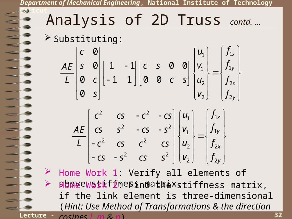
Substituting:
11
11
2 2
2 2
0
0 1 1 0 0
0 1 1 0 0
0
x
y
x
y
fucfvs c sAE
c c s u fL
s v f
2 211
2 211
2 22 2
2 22 2
x
y
x
y
fuc cs c csfvcs s cs sAE
u fL c cs c cs
v fcs s cs s
Home Work 1: Verify all elements of above stiffness matrix. Home Work 2: Find the stiffness matrix, if the link element
is three-dimensional (Hint: Use Method of Transformations & the direction cosines l, m & n)
Lecture - 03

33
Department of Mechanical Engineering, National Institute of Technology Calicut
Analysis of 2D Truss contd. …
Some Comments on Computer Implementation:
( ) ( ) ( ) ( ) ( )
( ) ( ) ( ) ( ) ( )
( ) ( ) ( ) ( ) ( )
( ) ( ) ( ) ( ) ( )
e e e e eiii ij ik il i
e e e e ejji jj jk jl j
e e e e ekki kj kk kl k
e e e e elli lj lk ll l
uk k k k f
uk k k k f
uk k k k f
uk k k k f
In a program, it is generally difficult to identify the direction of displacement or force.
The forces (or displacements) will be written as a single array, irrespective of the directions. Hence, we can write:
In other words, the x-displacement of node 2 is the 3rd element in the displacement vector (array).
Lecture - 03
34
Department of Mechanical Engineering, National Institute of Technology Calicut
Analysis of 2D Truss contd. …
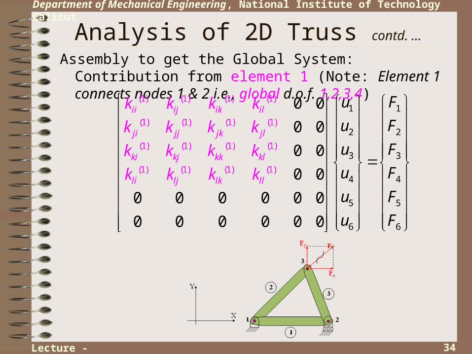
Assembly to get the Global System: Contribution from element 1 (Note: Element 1 connects nodes 1 & 2 i.e., global d.o.f. 1,2,3,4)
(1) (1) (1) (1)
(1) (1) (1) (1)
(1) (1) (1) (1)
(1) (1) (1) (1
1 1
2 2
3 3
4 4
5 5
)
6 6
0 0
0 0
0 0
0 0
0 0 0 0 0 0
0 0 0 0 0 0
ii ij ik il
ji jj jk jl
ki kj kk kl
li lj lk ll
k k k k
k k k k
k k k
u F
u F
uk F
uk k k k F
u F
u F
Lecture - 03
35
Department of Mechanical Engineering, National Institute of Technology Calicut
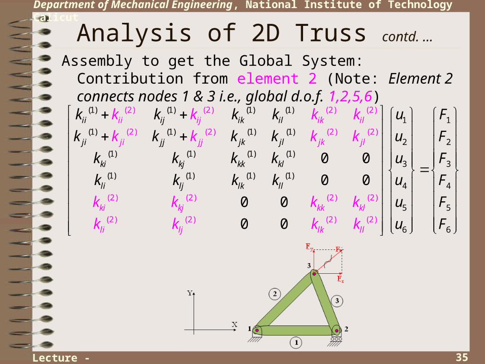
Analysis of 2D Truss contd. …
Assembly to get the Global System: Contribution from element 2 (Note: Element 2 connects nodes 1 & 3 i.e., global d.o.f. 1,2,5,6)
(1) (1) (1) (1)
(1) (1) (1) (1
(2) (2) (2) (2)
(2) (2) (2) (2)
(2) (2) (2) (2)
)
(1) (1) (1) (1)
(1) (1) (1) (1)
(2) (2) (2)
0 0
0 0
0 0
0 0
ii ij ik il
ji jj jk jl
ki kj kk kl
li lj lk ll
ii ij ik il
ji jj jk jl
ki kj kk kl
li lj lk l
k k k k
k k k k
k
k k k k
k k k k
k k k k
k
k k k
k k k k
k k k
1 1
2 2
3 3
4 4
5 5
6 6(2)
l
u F
u F
u F
u F
u F
u F
Lecture - 03

36
Department of Mechanical Engineering, National Institute of Technology Calicut
Analysis of 2D Truss contd. …
Finally, add the Contribution from element 3 (Note: Element 3 connects nodes 2 & 3 i.e., the global d.o.f. 3,4,5,6).
(1) (2) (1) (2) (1) (1) (2) (2)
(1) (2) (1) (2) (1) (1) (2) (2)
(1) (1) (1) (1)
(1) (1)
(3) (3) (3) (3)
(3) (3) (3) (3)(1) (1)
ii ii ij ij ik il ik il
ji ji jj jj jk jl jk jl
ki kj kk kl
li
ii ij ik il
ji jlj lk l j jk jl l
k k k k k k k k
k k k k k k k k
k k k k k
k k k
k k k
kk k k k
(3) (3) (3) (3)
1 1
2 2
3 3
4 4(2) (2) (2) (2)
5 5(2) (3) (3) (3) (3(2) (2) (2)
6 6)
ki kj kkki kj kk kl
l
kl
li lji lj l lk lk ll l
k k k k
k k k k
u F
u F
u F
u F
u Fk k k k
u Fk k k k
Lecture - 03

37
Department of Mechanical Engineering, National Institute of Technology Calicut
Concluding Remarks In the discrete systems, the elements and nodes are easily
identified – No Special Discretization procedure required. The governing equations are the linear algebraic equations in
terms of system variables – Directly Solvable. Some people do not consider Discrete system analysis as part
of “FEM”, since there is no numerical approximation of the distributions of primary variables.
In an introductory FEM course, the purposes served by studying discrete system analysis are:
1. Terminology – elemental & global stiffness matrix etc.
2. Concepts – Elements, Nodes, Primary variables etc.
3. The Assembly Process – Global & Local Coordinates, Global & Local Node numbering.
4. Application of Boundary Conditions & Solution.
Lecture - 03