ch 2 1 chapter 2 kinematics in one dimension giancoli, physics,6/e © 2004. electronically...
TRANSCRIPT

Ch 2 1
Chapter 2
Kinematics in One Dimension
Giancoli, PHYSICS,6/E © 2004. Electronically reproduced by permission of Pearson Education, Inc., Upper Saddle River, New Jersey
Ch 2 2
Module 2
Displacement, Velocity and Acceleration
Giancoli, Sec 2-1, 2, 3, 4, 8
AP Physics C Lesson 1
Giancoli, PHYSICS,6/E © 2004. Electronically reproduced by permission of Pearson Education, Inc., Upper Saddle River, New Jersey
The following is an excellent lecture on this material.
Ch 2 3
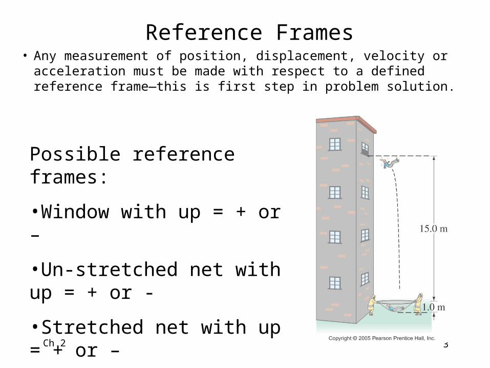
Reference Frames• Any measurement of position, displacement, velocity or
acceleration must be made with respect to a defined reference frame—this is first step in problem solution.
Possible reference frames:
•Window with up = + or –
•Un-stretched net with up = + or -
•Stretched net with up = + or –
•Ground = not sufficient information
Ch 2 4
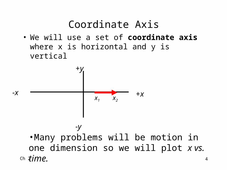
Coordinate Axis• We will use a set of coordinate axis where x is
horizontal and y is vertical
+y
-y
+x-xx1 x2
•Many problems will be motion in one dimension so we will plot x vs. time.
Ch 2 5
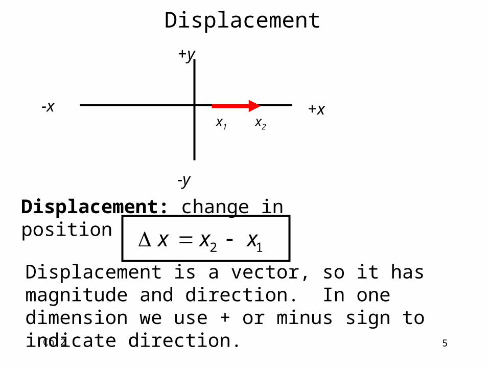
Displacement
Displacement: change in position
12 xxx
+y
-y
+x-xx1 x2
Displacement is a vector, so it has magnitude and direction. In one dimension we use + or minus sign to indicate direction.
Ch 2 6
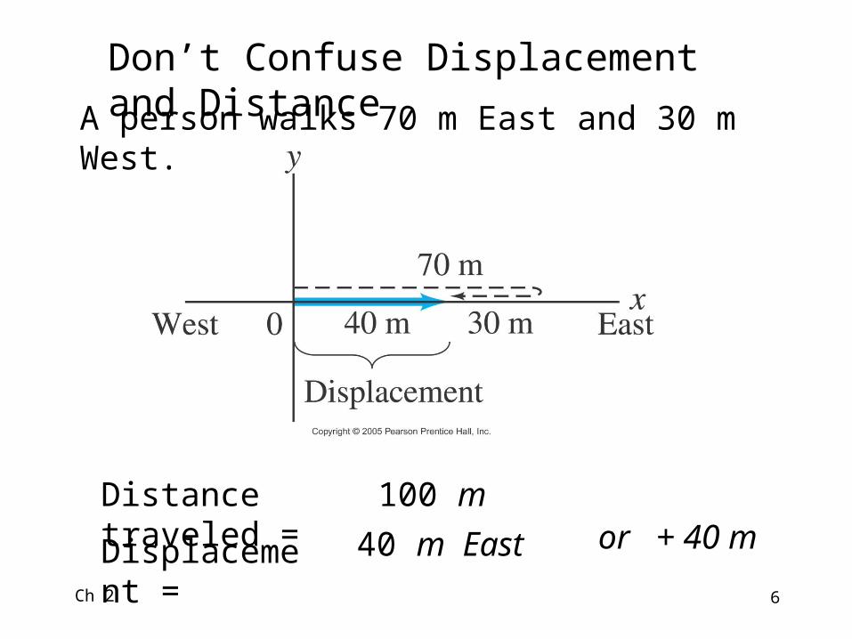
Don’t Confuse Displacement and Distance
A person walks 70 m East and 30 m West.
Distance traveled =
Displacement =
100 m
40 m East or + 40 m
Ch 2 7
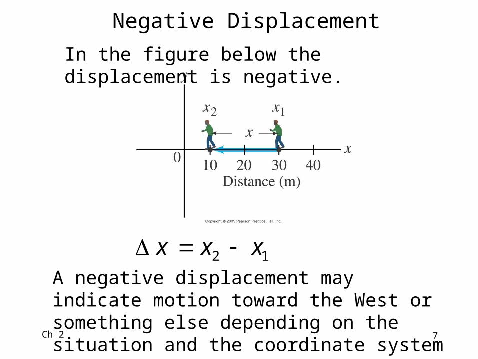
Negative Displacement
In the figure below the displacement is negative.
A negative displacement may indicate motion toward the West or something else depending on the situation and the coordinate system chosen.
12 xxx

Ch 2 8
Average Speed and Velocity
elapsed time
traveleddistance speed average
elapsed time
nt displaceme( velocity average )v
t
x
tt
xxv
12
12
Average velocity is a vector, so it has magnitude and direction. In one dimension we use + or minus sign to indicate direction.

Ch 2 9
t
x
t
xv
21ttt
hkm
km
hkm
kmt
990
2800
790
3100
Example 1. An airplane travels 3100 km at a speed of 790 km/h, and then encounters a tailwind that boosts its speed to 990 km/h for the next 2800 km. What was the total time for the trip? (Assume three significant figures)
hhht 75.683.292.3
2
2
1
1
v
x
v
xt

Ch 2 10
Example 1 (continued) An airplane travels 3100 km at a speed of 790 km/h, and then encounters a tailwind that boosts its speed to 990 km/h for the next 2800 km. What was the total time for the trip? (Assume three significant figures)
What was the average speed of the plane for this trip?
ht 75.6
t
xv
h
kmkm
75.6
28003100 h
km874
Note: A simple average of v1 and v2 gives 890 km/h and is not correct
Ch 2 11
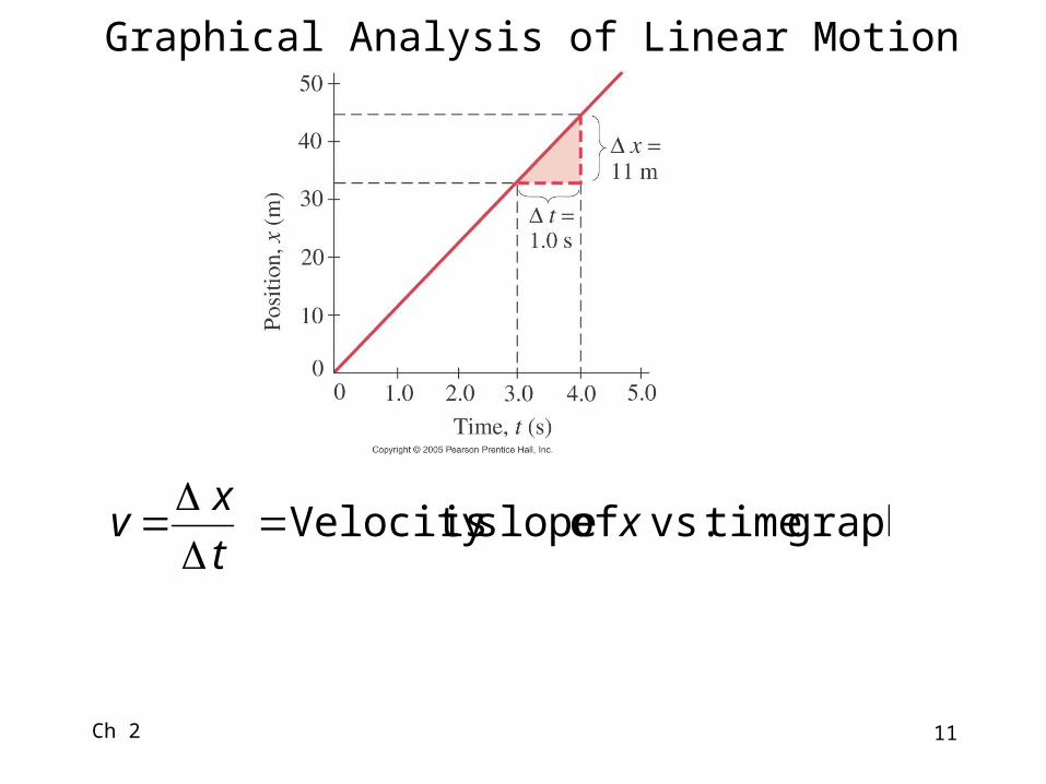
Graphical Analysis of Linear Motion
graphtimevs. of slope isVelocity xt
xv
Ch 2 12
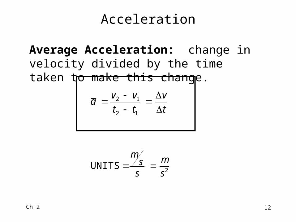
Acceleration
Average Acceleration: change in velocity divided by the time taken to make this change.
t
v
tt
vva
12
12
2 UNITS
s
m
ss
m

Ch 2 13
smvst
smvt
0.50.5
0.150
22
11
12
12
tt
vva
sss
ms
m
00.5
0.150.5
Example 2. A car traveling at 15.0 m/s slows down to 5.0 m/s in 5.0 seconds. Calculate the car’s acceleration.
Coordinate System: + is to the right
20.2s
m )left theto(
Ch 2 14
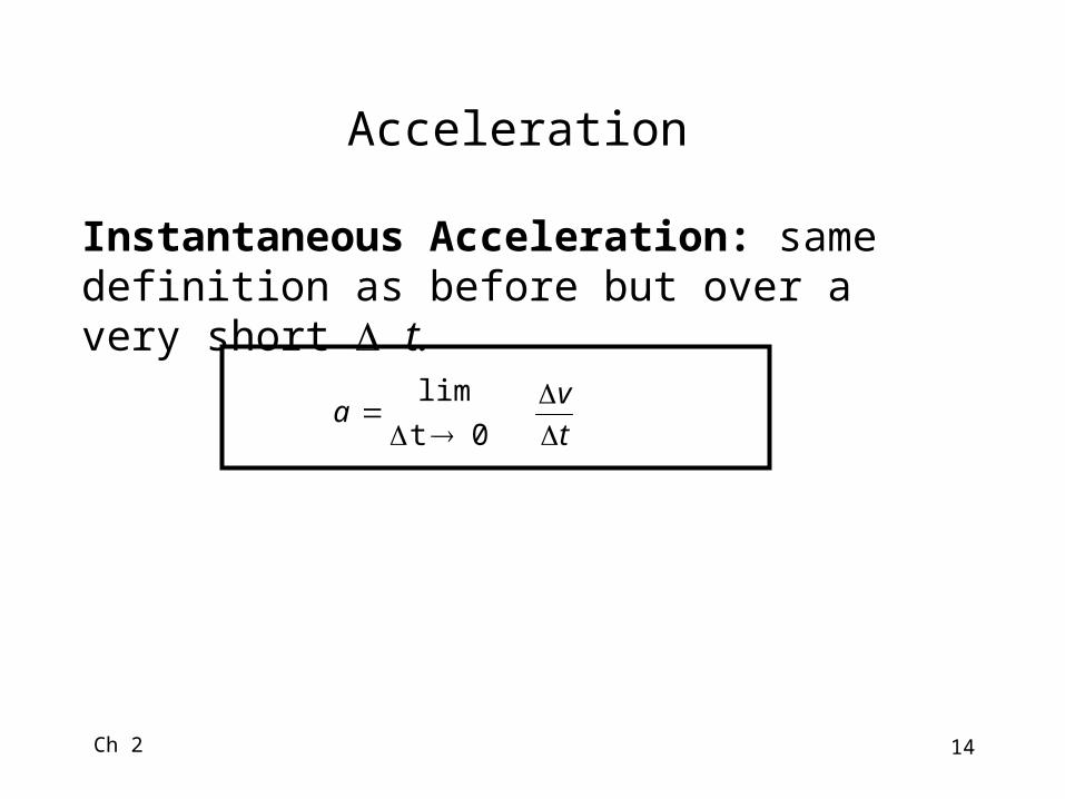
Acceleration
Instantaneous Acceleration: same definition as before but over a very short t.
t
va
0t
lim
Ch 2 15
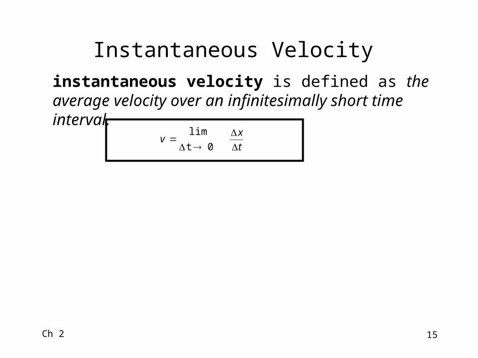
Instantaneous Velocity
instantaneous velocity is defined as the average velocity over an infinitesimally short time interval.
t
xv
0t
lim

Ch 2 16
Graphical Analysis of Linear Motion
graphtimevs. of slope ison Accelerati vt
va

Ch 2 17
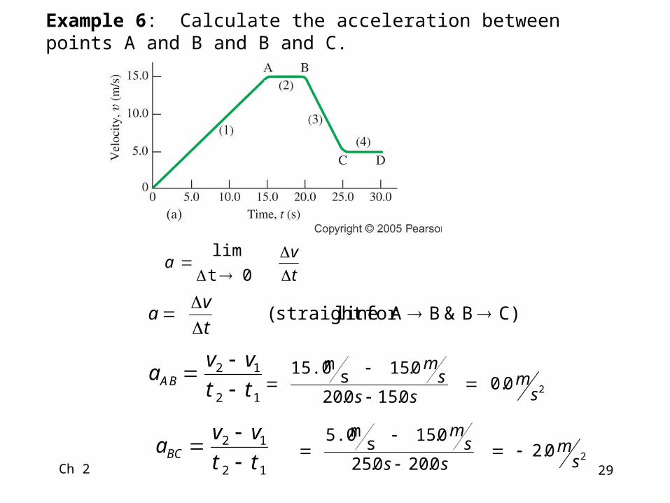
Example 6: Calculate the acceleration between points A and B and B and C.
t
va
0t
lim
) linestraight (t
va
20.00.150.20
0.15sm15.0
sm
sss
m
12
12
tt
vva BA
20.20.200.25
0.15sm5.0
sm
sss
m
12
12
tt
vvaBC
Ch 2 18
Module 3
Motion with Constant Acceleration
Giancoli, Sec 2-1, 2, 3, 4, 8
Giancoli, PHYSICS,6/E © 2004. Electronically reproduced by permission of Pearson Education, Inc., Upper Saddle River, New Jersey
Ch 2 19
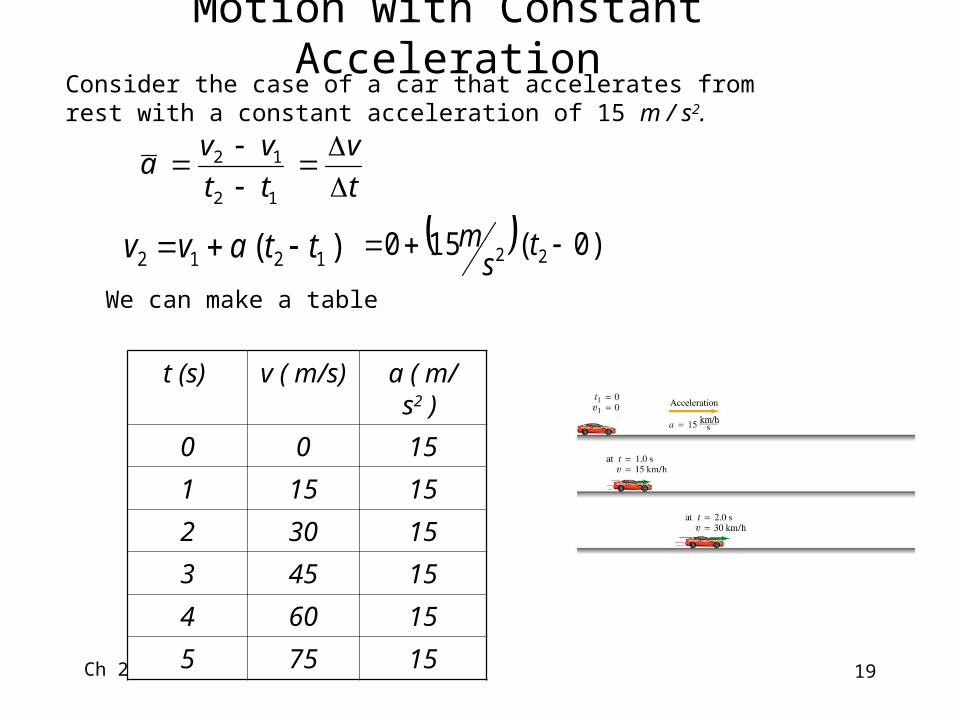
Motion with Constant Acceleration
t (s) v ( m/s) a ( m/ s2 )
0 0 15
1 15 15
2 30 15
3 45 15
4 60 15
5 75 15
Consider the case of a car that accelerates from rest with a constant acceleration of 15 m / s2.
t
v
tt
vva
12
12
)( 1212 ttavv )0(150 22 ts
m
We can make a table
Ch 2 20
Derivations•In the next 4 slides we will combine several known equations under the assumption that the acceleration is constant.
•This process is called a derivation.
•In general you will need to know the initial assumptions, the resultant equations and how to apply them.
•You do not need to memorize derivations
•But, I could ask you to derive an equation for a specific problem. This is very similar to an ordinary problem without a numeric answer.
Ch 2 21
Motion at Constant Acceleration - Derivation
•Consider the special case acceleration equals a constant: a = constant
• Use the subscript “0” to refer to the initial conditions
• Thus t0 refers to the initial time and we will set t0 = 0.
• At this time v0 is the initial velocity and x0 is the initial displacement.
•At a later time t, v is the velocity and x is the displacement
•In the equations t1t0 and t2 t
Ch 2 22
Motion at Constant Acceleration - Derivation
1)(Eqn.0
0
0
t
xx
tt
xxv
) 2 Eqn.(Constant0
t
vva
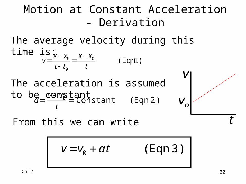
The average velocity during this time is:
The acceleration is assumed to be constant
From this we can write
) 3 Eqn. (0 tavv
t
v
ov

Ch 2 23
Motion at Constant Acceleration - DerivationBecause the velocity increases at a uniform rate, the average velocity is the average of the initial and final velocities
)4Eqn.(2
0 vvv
From the definition of average velocity
tatvv
xtvv
xtvxx )2
()2
( 000
000
And thus
)5Eqn.(2
1 200 tatvxx
t
v
ov
Ch 2 24
Motion at Constant Acceleration
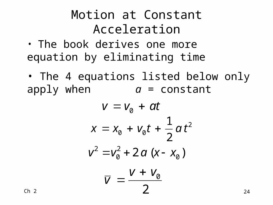
• The book derives one more equation by eliminating time
• The 4 equations listed below only apply when a = constant
tavv 0
200 2
1tatvxx
)(2 020
2 xxavv
20vv
v
Ch 2 25
mxsmv
xv
0.155.11
0000
0
2
0
2 2 xxavv
)(20
2
0
2
xx
vva
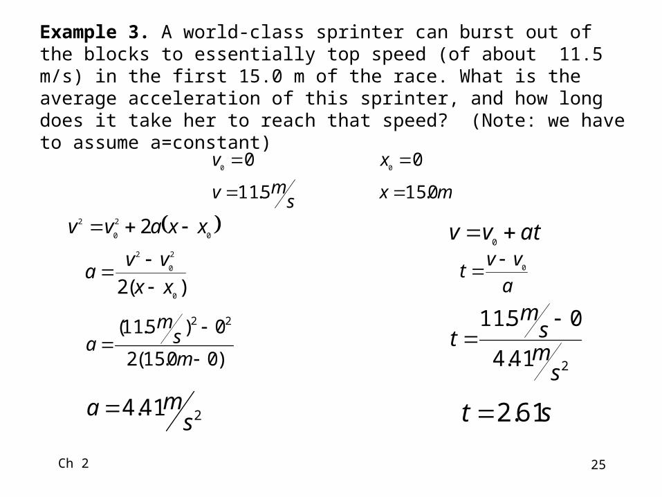
Example 3. A world-class sprinter can burst out of the blocks to essentially top speed (of about 11.5 m/s) in the first 15.0 m of the race. What is the average acceleration of this sprinter, and how long does it take her to reach that speed? (Note: we have to assume a=constant)
)00.15(2
0)5.11( 22
ms
ma
241.4s
ma
atvv 0
a
vvt 0
241.4
05.11
sms
mt
st 61.2
Ch 2 26
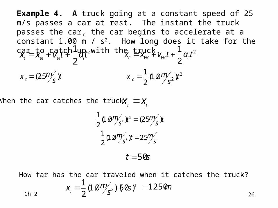
2
00 2
1tatvxx
tttt
tsmx t )25(
200 2
1tatvxx cccc
Example 4. A truck going at a constant speed of 25 m/s passes a car at rest. The instant the truck passes the car, the car begins to accelerate at a constant 1.00 m / s2. How long does it take for the car to catch up with the truck.
How far has the car traveled when it catches the truck?
22 )0.1(
2
1t
smx c
When the car catches the truck:tc
xx
tsmts
m )25()0.1(2
1 22
smts
m 25)0.1(2
12
st 50
22 )50)(0.1(
2
1ss
mxc m1250
Ch 2 27
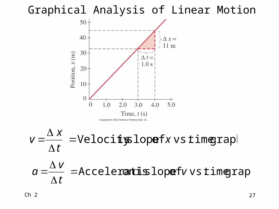
Graphical Analysis of Linear Motion
graphtimevs. of slope isVelocity xt
xv
graphtimevs. of slope ison Accelerati vt
va
Ch 2 28
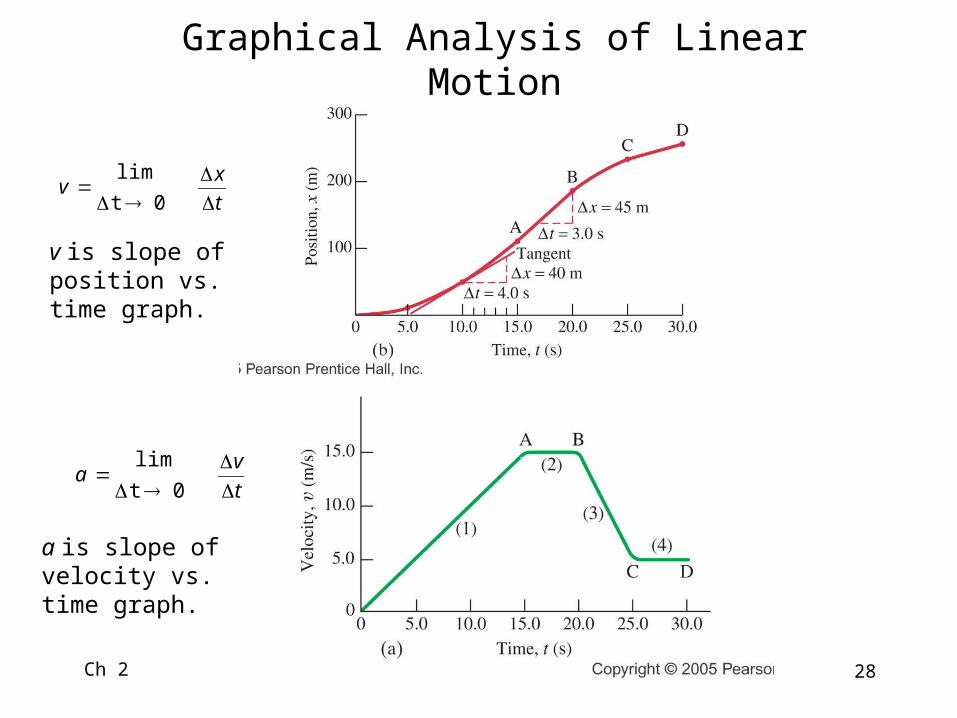
Graphical Analysis of Linear Motion
t
xv
0t
lim
t
va
0t
lim
v is slope of position vs. time graph.
a is slope of velocity vs. time graph.
Ch 2 29
Example 6: Calculate the acceleration between points A and B and B and C.
t
va
0t
lim
C) B & B A for linestraight (
t
va
20.00.150.20
0.15sm15.0
sm
sss
m
12
12
tt
vva BA
20.20.200.25
0.15sm5.0
sm
sss
m
12
12
tt
vvaBC
Ch 2 30
Module 4
Falling Objects
Giancoli, Sec 2-1, 2, 3, 4, 8
Giancoli, PHYSICS,6/E © 2004. Electronically reproduced by permission of Pearson Education, Inc., Upper Saddle River, New Jersey
Ch 2 31
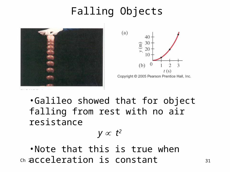
Falling Objects
•Galileo showed that for object falling from rest with no air resistance
y t2
•Note that this is true when acceleration is constant
Ch 2 32
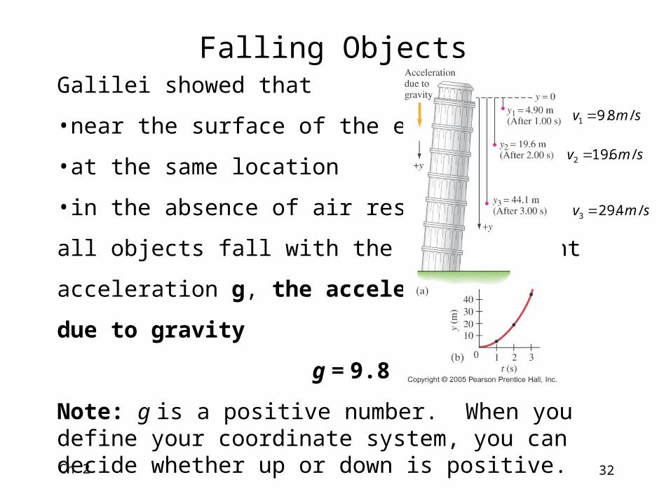
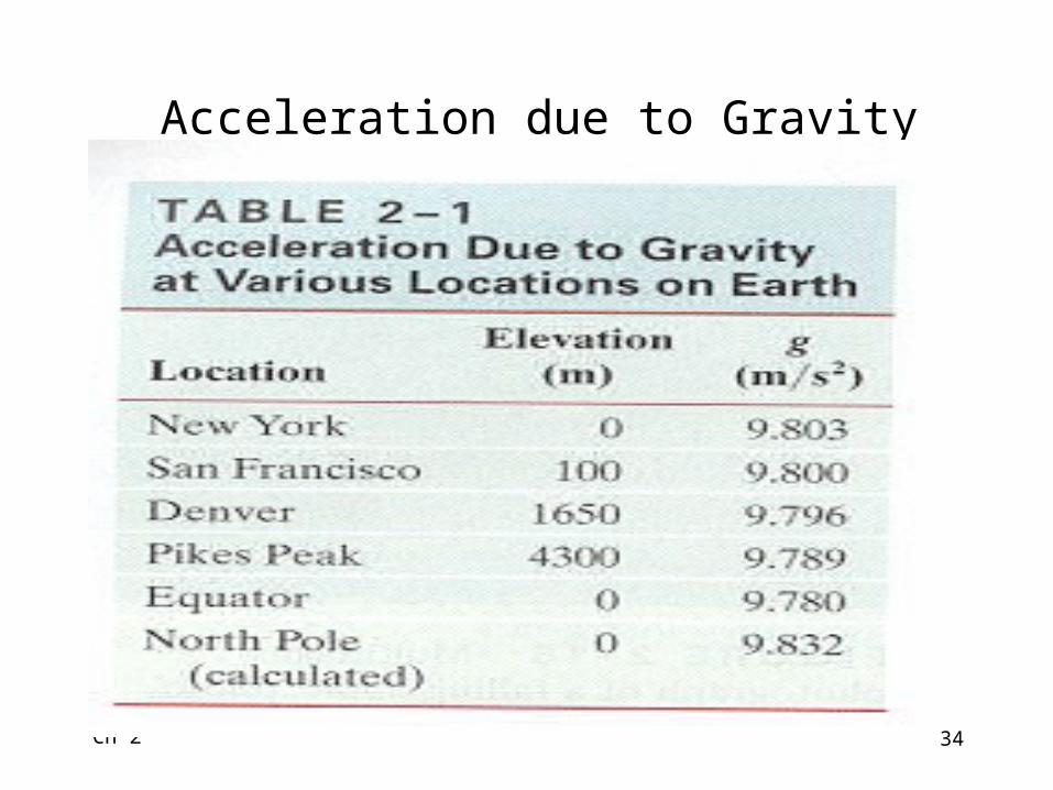
Falling ObjectsGalilei showed that
•near the surface of the earth
•at the same location
•in the absence of air resistance
all objects fall with the same constant
acceleration g, the acceleration
due to gravity
g = 9.8 m/s2
Note: g is a positive number. When you define your coordinate system, you can decide whether up or down is positive.
smv /8.91
smv /6.192
smv /4.293

Ch 2 33
Up and Down Motion
For object that is thrown upward and returns to starting position:
• assumes up is positive
•velocity changes sign (direction) but acceleration does not
•Velocity at top is zero
•time up = time down
•Velocity returning to starting position = velocity when it was released but opposite sign
2
00 2
1gttvyy
gtvv 0
Ch 2 34
Acceleration due to Gravity
Ch 2 35
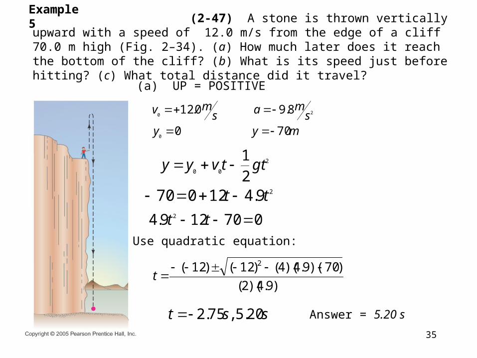
Example 5
myys
masmv
700
8.90.12
0
20
2
00 2
1gttvyy
29.412070 tt
(2-47) A stone is thrown vertically upward with a speed of 12.0 m/s from the edge of a cliff 70.0 m high (Fig. 2–34). (a) How much later does it reach the bottom of the cliff? (b) What is its speed just before hitting? (c) What total distance did it travel?
(a) UP = POSITIVE
070129.4 2 tt
)9.4)(2(
)70)(9.4)(4()12()12( 2 t
sst 20.5,75.2
Use quadratic equation:
Answer = 5.20 s
Ch 2 36
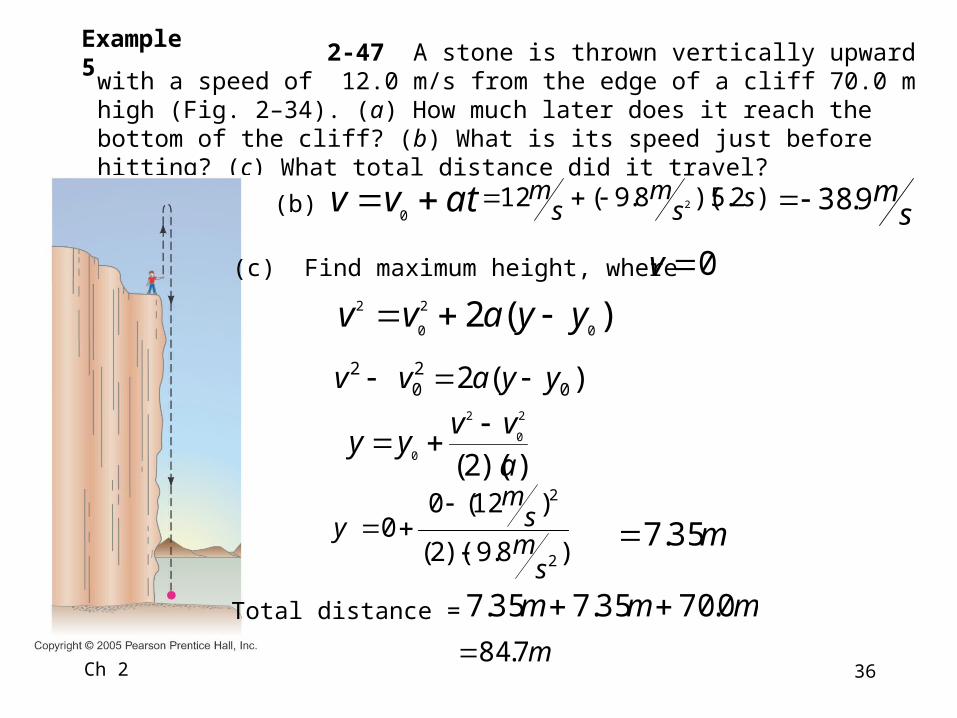
Example 5
atvv 0
)2.5)(8.9(12 2 ssm
sm
2-47 A stone is thrown vertically upward with a speed of 12.0 m/s from the edge of a cliff 70.0 m high (Fig. 2–34). (a) How much later does it reach the bottom of the cliff? (b) What is its speed just before hitting? (c) What total distance did it travel?
(b) sm9.38
(c) Find maximum height, where 0v
)(20
2
0
2 yyavv
))(2(
2
0
2
0 a
vvyy
)8.9)(2(
)12(00
2
2
sms
my
m35.7
Total distance = mmm 0.7035.735.7 m7.84
)(2 020
2 yyavv
Ch 2 37
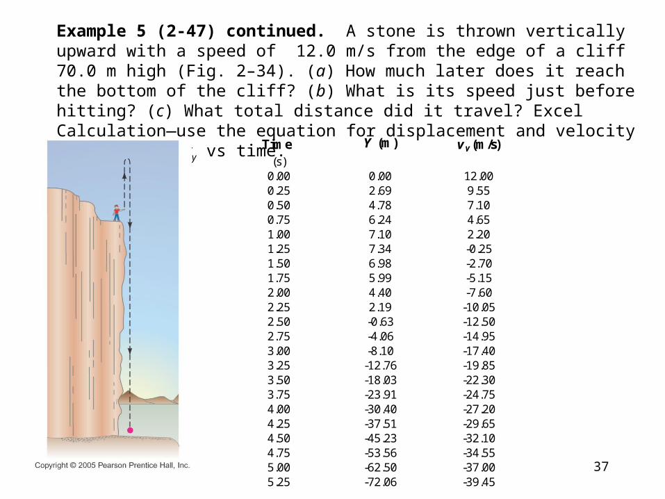
Example 5 (2-47) continued. A stone is thrown vertically upward with a speed of 12.0 m/s from the edge of a cliff 70.0 m high (Fig. 2–34). (a) How much later does it reach the bottom of the cliff? (b) What is its speed just before hitting? (c) What total distance did it travel? Excel Calculation—use the equation for displacement and velocity to get y and vy vs time.
Time Y (m) v y (m/s)(s)
0.00 0.00 12.000.25 2.69 9.550.50 4.78 7.100.75 6.24 4.651.00 7.10 2.201.25 7.34 -0.251.50 6.98 -2.701.75 5.99 -5.152.00 4.40 -7.602.25 2.19 -10.052.50 -0.63 -12.502.75 -4.06 -14.953.00 -8.10 -17.403.25 -12.76 -19.853.50 -18.03 -22.303.75 -23.91 -24.754.00 -30.40 -27.204.25 -37.51 -29.654.50 -45.23 -32.104.75 -53.56 -34.555.00 -62.50 -37.005.25 -72.06 -39.45

Ch 2 38
Problem Solving Tips1. Read the whole problem and make sure you
understand it. Then read it again.
2. Decide on the objects under study and what the time interval is.
3. Draw a diagram and choose coordinate axes.
4. Write down the known (given) quantities, and then the unknown ones that you need to find.
5. What physics applies here? Plan an approach to a solution.

Ch 2 39
Problem Solving Tips6. Which equations relate the known and unknown quantities? Are they valid in this situation? Solve algebraically for the unknown quantities, and check that your result is sensible (correct dimensions).
7. Calculate the solution and round it to the appropriate number of significant figures.
8. Look at the result – is it reasonable? Does it agree with a rough estimate?
9. Check the units again.