CFD General Notation System (CGNS)

Tutorial Session

2

Agenda• 7:00-7:30 Introduction, overview, and basic usage

C. Rumsey (NASA Langley)• 7:30-7:50 Usage for structured grids

B. Wedan (ANSYS – ICEM)• 7:50-8:10 Usage for unstructured grids

E. van der Weide (Stanford University)• 8:20-8:40 HDF5 usage and parallel implementation

T. Hauser (Utah State University)• 8:40-9:00 Python and in-memory CGNS trees

M. Poinot (ONERA)• 9:00-9:30 Discussion and question/answer period

CFD General Notation System (CGNS)Introduction, overview, and basic usage

Christopher L. RumseyNASA Langley Research Center

Chair, CGNS Steering Committee

4

Outline• Introduction • Overview of CGNS

– What it is– History– How it works, and how it can help– The future

• Basic usage– Getting it and making it work for you– Simple example– Aspects for data longevity

5

Introduction

• CGNS provides a general, portable, and extensible standard for the storage and retrieval of CFD analysis data

• Principal target is data normally associated with computed solutions of the Navier-Stokes equations & its derivatives

• But applicable to computational field physics in general (with augmentation of data definitions and storage conventions)

6

What is CGNS?• Standard for defining & storing CFD data

– Self-descriptive– Machine-independent– Very general and extendable– Administered by international steering committee

• AIAA recommended practice (AIAA R-101-2002)• In process of becoming part of international ISO

standard• Free and open software• Well-documented• Discussion forum: cgnstalk@lists.nasa.gov• Website: http://www.cgns.org

7

History

• CGNS was started in the mid-1990s as a joint effort between NASA, Boeing, and McDonnell Douglas– Under NASA’s Advanced Subsonic Technology (AST)

program• Arose from need for common CFD data format for

improved collaborative analyses between multiple organizations– Existing formats, such as PLOT3D, were incomplete,

cumbersome to share between different platforms, and not self-descriptive (poor for archival purposes)

• Initial development was heavily influenced by McDonnell Douglas’ “Common File Format”, which had been in use since 1989

• Version 1.0 of CGNS released in May 1998

8

History, cont’d

• After AST funding ended in 1999, CGNS steering committee was formed– Voluntary public forum– International members from government, industry, academia– Formally became a sub-committee of AIAA Committee on

Standards in 2000• Initial efforts by Boeing to make CGNS an

international ISO-STEP standard (1999-2002) – Stalled due to lack of funding– Instead, the existing ISO standard AP209 (finite element

solid mechanics) is being rewritten (AP209E2) to include CGNS as well as an integrated engineering analysis framework (headed by Lockheed-Martin)

9

Steering committee

• CGNS Steering committee is a public forum• Responsibilities include (1) maintaining software,

documentation, and website, (2) ensuring free distribution, and (3) promoting acceptance

• Current steering committee make-up (20 members):ADAPCO

ANSYS-CFX

Aerospatiale Matra Airbus

Boeing – IDS/PW

Boeing Commercial

Boeing IDS

Fluent

ANSYS-ICEM

Intelligent Light

NASA Glenn

NASA Langley

ONERA

Pacific NW Laboratory

Pointwise

Pratt & Whitney

Pratt & Whitney – Rocketdyne

Rolls-Royce Allison

Stanford University

U.S. Air Force / AEDC

Utah State University

10

CGNS main features• Hierarchical data structure : quickly traversed and

sorted, no need to process irrelevant data• Files stored in compact C binary format• Layered so that many of the data structures are

optional• ADF or HDF5 database: universal and self-describing• Data may encompass multiple files through the use

of links• Portable ANSI C software, with complete Fortran and

C interfaces• Architecture-independent application programming

interface (API) – written as a mid-level library (MLL)

11

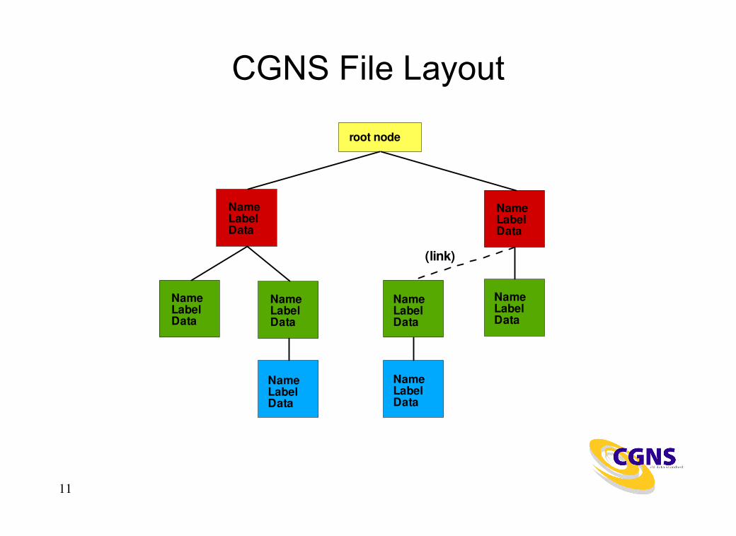
CGNS File Layout

root node

NameLabelData

NameLabelData

NameLabelData

NameLabelData

NameLabelData

NameLabelData

NameLabelData

(link)

NameLabelData

12

Makeup of CGNS• Standard Interface Data Structures (SIDS) is the core of CGNS –

defines the intellectual content– Defines what goes in the “boxes” and how they are organized

• Original low level implementation is Advanced Data Format (ADF)– Basic direct I/O operations– Software has no knowledge of data structure or contents– Tree-based (nodal parent/child) structure

• Low level implementation is migrating toward HDF5 format– HDF5 is already available as an option– HDF5 is well-supported (NCSA) , widely used, and has parallel I/O

capability– This will be the official recommended format, although ADF will also

continue to be supported, and MLL will translate between the two• Mid-level library (MLL) is currently available for C and Fortran

– This is what most users employ– Software has some knowledge of SIDS– C++ and Python extensions also available

13

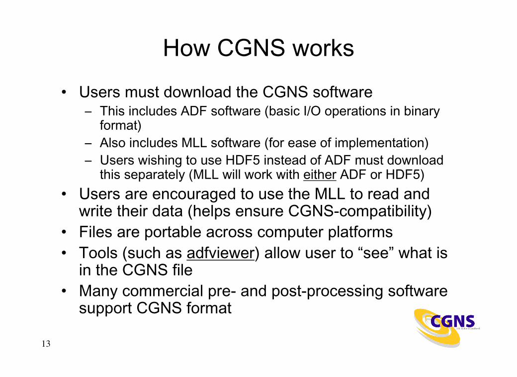
How CGNS works

• Users must download the CGNS software– This includes ADF software (basic I/O operations in binary

format)– Also includes MLL software (for ease of implementation)– Users wishing to use HDF5 instead of ADF must download

this separately (MLL will work with either ADF or HDF5)• Users are encouraged to use the MLL to read and

write their data (helps ensure CGNS-compatibility)• Files are portable across computer platforms• Tools (such as adfviewer) allow user to “see” what is

in the CGNS file• Many commercial pre- and post-processing software

support CGNS format

14

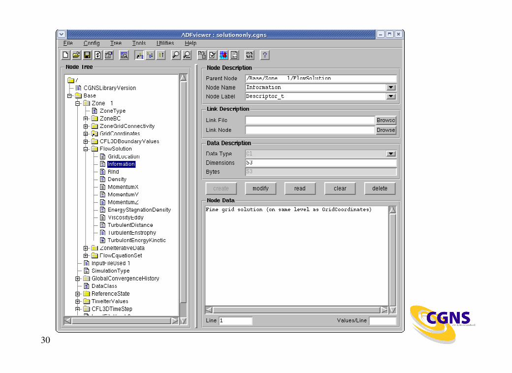
Typical view of CGNS file using ADFVIEWER

15

Typical CGNS file

Root node

CGNSBase_tCGNSLibraryVersion_t

Zone 1 Zone 2 ConvergenceHistory_t ReferenceState_t

GridCoordinates_tElements_t FlowSolution_t ZoneGridConnectivity_t

Zone_t Zone_t

ElementConnectivity CoordinateY

DataArray_t DataArray_t

GridLocation Density Pressure

GridLocation_t DataArray_t DataArray_t

ZoneBC_t

CoordinateX

DataArray_t

16

Cons and Pros• Cons

– Although there are rules, there are also many options and a certain amount of freedom

• Example: GridLocation = Vertex vs. CellCenter• Example: data can be stored dimensional or nondimensional• Example: optional use of Rind cells

– This flexibility places more responsibility on the CGNS reader to figure out how to make use of what is in the file

– Attempted balance between too rigid and too flexible• Pros

– As more people use it, more tools get developed to handle the flexibility

– Can be as simple as storing only “grid + flow solution”, or as complex as storing everything needed to run/describe a case

– Longevity and infinite extensibility

17

How CGNS can help you• Improves longevity (archival quality) of data

– Self-descriptive (more on this later)– Machine-independent

• Easy to share data files between sites– Eliminates need to translate between different data formats– Rigorous standard means less ambiguity about what the data

means• Saves time and money

– For example, easy to set-up CFD runs because files include grid coordinates, connectivity, and BC information

• Easily extendible to include additional types of data– Solver-specific or user-specific data can easily be written &

read – file remains CGNS-compliant (others can still read it!)– Once defined & agreed upon, new data standards can be

added

18

Status/where CGNS is headed• Latest version is 2.4• As of Aug 2005, the CGNSTalk mailing list had 161 participants

from 21 different countries and at least 80 different organizations• Over 11,000 CGNS downloads from SourceForge over last 3

years (average of 408 per month over last 1 year)• Many people have expressed interest in CGNS from outside of

the traditional aerodynamics community– E.g., computational physiology, electromagnetics

• Parallel I/O (through HDF5) will be available soon• CGNS is already in many widely-used commercial visualization

products, e.g., Tecplot, Fieldview, ICEM-CFD (reader for Paraview being worked)

• Continuous process: approval and implementation of extensions for handling new capabilities

19

Getting CGNS

• Go to http://www.cgns.org and follow instructions– Or go directly to http://www.SourceForge.net– You can get the official released version (currently 2.4), or

use CVS to keep up with the latest fixes– E.g.: cgnslib_2.4-4.tar.gz (or cgnslib_2.4-4.zip for Windows)– Follow instructions in README file to compile

• Also highly recommended (from same place):– cgnstools (tools for viewing/editing)– CGNS Users Guide (practical entry-level manual for getting

started with CGNS – includes simple source codes)

20

Basics of using CGNS• Simple example: opening, closing, writing, &

reading Base• Aspects for data longevity

– Boundary conditions– Convergence history– Descriptor nodes– Data & equation descriptions– Flowfield variables

21

Opening/closing file & writing Base• C

cg_open(“grid.cgns”, MODE_WRITE, &indexf);basename=“Base”;icelldim=3; /* dimensionality of cell (3 for volume cell) */iphysdim=3; /* number of coordinates (3 for 3-D) */cg_base_write(indexf, basename, icelldim, iphysdim, &indexb);

……..cg_close(indexf);

• Fortrancall cg_open_f(‘grid.cgns’, MODE_WRITE, indexf, ier)basename=‘Base’icelldim=3iphysdim=3call cg_base_write_f(indexf, basename, icelldim, iphysdim, indexb, ier)

……..call cg_close_f(indexf, ierr)

22

What the file looks like…

Root node

Name = BaseLabel = CGNSBase_tData = 3, 3

Name = CGNSLibraryVersionLabel = CGNSLibraryVersion_tData = 2.4

automatic

automatic automatic

user-defined

Notes: icelldim = dimensionality of cell (2 for face, 3 for volume)iphysdim = no. of coordinates required to define a node

position (1 for 1-D, 2 for 2-D, 3 for 3-D)

23

What the file looks like in adfviewer…

24

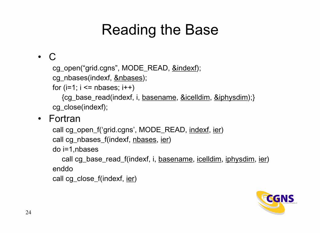
Reading the Base

• Ccg_open(“grid.cgns”, MODE_READ, &indexf);cg_nbases(indexf, &nbases);for (i=1; i <= nbases; i++)

{cg_base_read(indexf, i, basename, &icelldim, &iphysdim);}cg_close(indexf);

• Fortrancall cg_open_f(‘grid.cgns’, MODE_READ, indexf, ier)call cg_nbases_f(indexf, nbases, ier)do i=1,nbases

call cg_base_read_f(indexf, i, basename, icelldim, iphysdim, ier)enddocall cg_close_f(indexf, ier)

25

Aspects for data longevityboundary conditions

• BCs are included in the CGNS file• Including BCs makes it easier for someone

else to duplicate the same flow conditions• Eliminates doubt as to how the solution was

run, when later looking at the file• BCs can be simple or have high level of detail

– Minimum: list of points and their BC type (name)– Can also include Dirichlet or Neumann-type data

26

27

Aspects for data longevityconvergence history

• GlobalConvergenceHistory tracks history of residual(s), forces, moments, etc.

• Part of a complete record of the flow solution, easily readable by others

28

29

Aspects for data longevitydescriptor nodes

• Allow user to add notes, descriptions, important factors associated with the particular run, etc.

• As part of the permanent record, descriptor nodes make the file potentially more useful/meaningful in the future

• Full inclusion of flow solver input deck(s) is particularly useful

• Eliminates doubt as to how the solution was run, when later looking at the file

30

31

32

Aspects for data longevitydata & equation descriptions

• Documents the dimensionality & units (or normalization) of the data

• Reference state and flow solution method become part of permanent record

• Eliminates doubt as to what the variables represent and how the solution was run, when later looking at the file

33

34

35

36

Aspects for data longevityflowfield variables

• As many flowfield variables as desired can be stored; for example:– Conserved and/or primitive variables– Plus all turbulence quantities, eddy viscosity,

distance functions, species mass fractions, or other flowfield quantities of interest

• Eliminates having to go back and restart or reconstruct when you want to obtain non-standard quantities

37

Some final comments• A CGNS file can be as full or as sparse as

you want to make it– The fuller it is, the more complete and archival the

file– Always easy to read only the parts you want

• Easy to build CGNS into existing processes– Start by writing only the “basic” elements of CGNS

file (e.g., grid, flow solution, connectivity, and BCs) as a postprocessing file for flow visualization

– Gradually add to completeness of file– Eventually, CGNS file can replace your restart file,

if desired

38

Conclusions• CGNS is a well-established, stable format with world-

wide acceptance, use, and support• Provides seamless communication of data between

applications, sites, and system architectures• Supported by many commercial visualization and

CFD vendors• Extensible and flexible – easily adapted to other fields

of computational physics through specification in the SIDS

• Backward compatible with previous versions; forward compatible within major release numbers

• Allows new software development to focus on important matters, rather than on time-consuming data I/O, storage, and compatibility issues

39

Conclusions, cont’d

• CGNS is the best thing since sliced bread!

Auxiliary slides

41

Writing structured gridsdouble x[kdim][kdim][idim], y[kdim][jdim][idim], z[kdim][jdim][idim];int isize[3][3];strcpy(zonename,”Zone 1”);/* vertex size (structured grid example) */isize[0][0]=idim;isize[0][1]=jdim;isize[0][2]=kdim;/* cell size (structured grid example) */isize[1][0]=isize[0][0]-1;isize[1][1]=isize[0][1]-1;isize[1][2]=isize[0][2]-1;/* boundary vertex size (always zero for structured) */isize[2][0]=0;isize[2][1]=0;isize[2][2]=0;

42

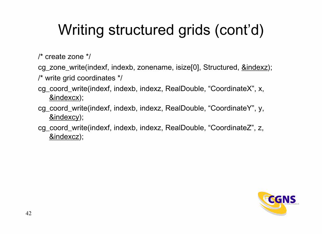
Writing structured grids (cont’d)/* create zone */cg_zone_write(indexf, indexb, zonename, isize[0], Structured, &indexz);/* write grid coordinates */cg_coord_write(indexf, indexb, indexz, RealDouble, “CoordinateX”, x,

&indexcx);cg_coord_write(indexf, indexb, indexz, RealDouble, “CoordinateY”, y,

&indexcy);cg_coord_write(indexf, indexb, indexz, RealDouble, “CoordinateZ”, z,

&indexcz);

43

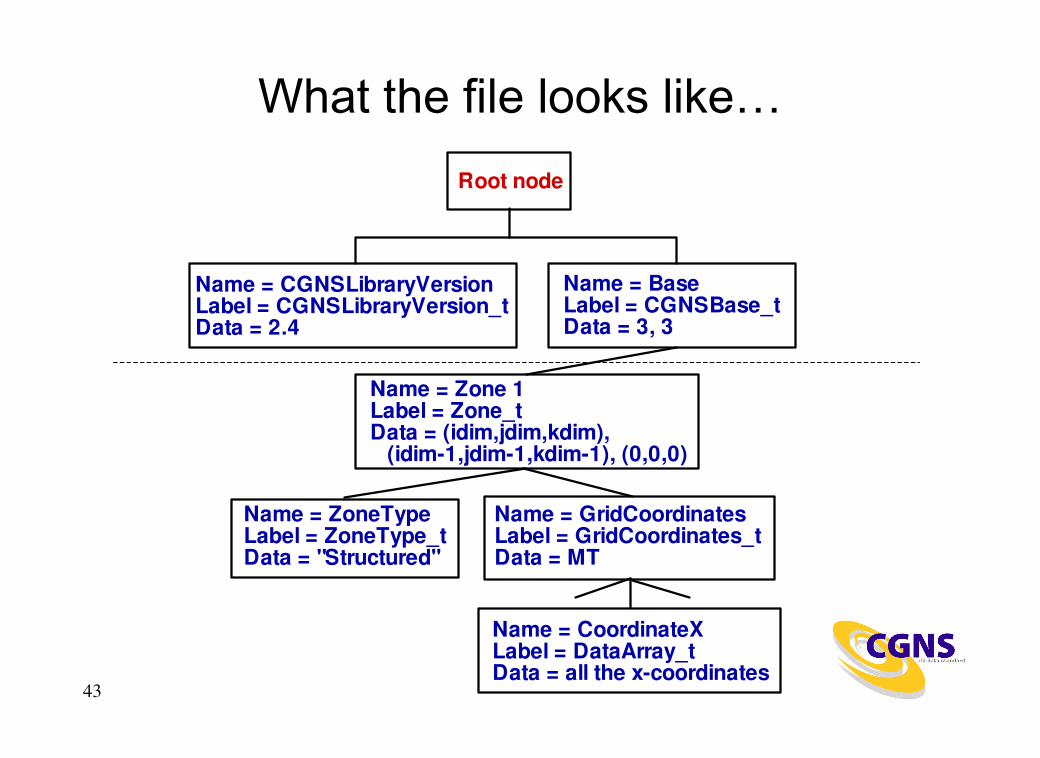
What the file looks like…Root node

Name = Zone 1Label = Zone_tData = (idim,jdim,kdim),

(idim-1,jdim-1,kdim-1), (0,0,0)

Name = CGNSLibraryVersionLabel = CGNSLibraryVersion_tData = 2.4

Name = BaseLabel = CGNSBase_tData = 3, 3

Name = ZoneTypeLabel = ZoneType_tData = "Structured"

Name = GridCoordinatesLabel = GridCoordinates_tData = MT

Name = CoordinateXLabel = DataArray_tData = all the x-coordinates

44

What the file looks like in adfviewer…

45

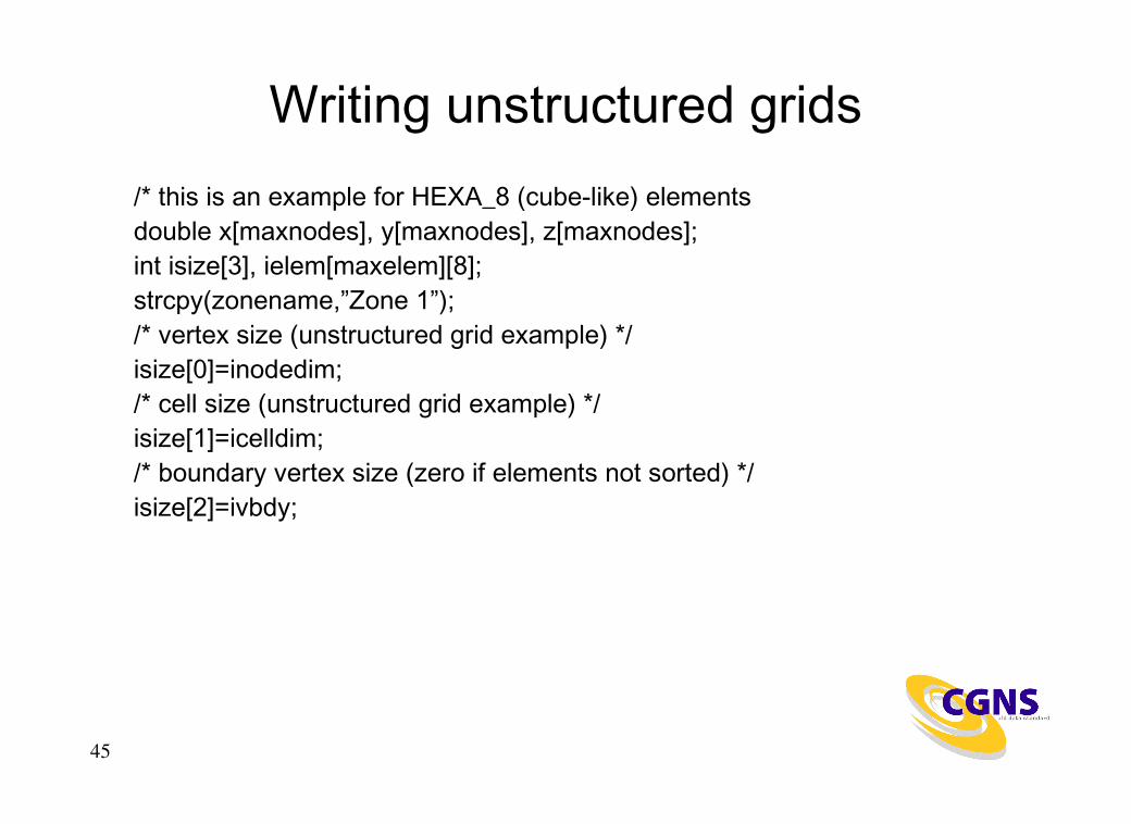
Writing unstructured grids/* this is an example for HEXA_8 (cube-like) elementsdouble x[maxnodes], y[maxnodes], z[maxnodes];int isize[3], ielem[maxelem][8];strcpy(zonename,”Zone 1”);/* vertex size (unstructured grid example) */isize[0]=inodedim;/* cell size (unstructured grid example) */isize[1]=icelldim;/* boundary vertex size (zero if elements not sorted) */isize[2]=ivbdy;

46

Writing unstructured grids (cont’d)/* create zone */cg_zone_write(indexf, indexb, zonename, isize, Unstructured, &indexz);/* write grid coordinates */cg_coord_write(indexf, indexb, indexz, RealDouble, “CoordinateX”, x,

&indexcx);cg_coord_write(indexf, indexb, indexz, RealDouble, “CoordinateY”, y,

&indexcy);cg_coord_write(indexf, indexb, indexz, RealDouble, “CoordinateZ”, z,

&indexcz);/* write element connectivity */cg_section_write(indexf, indexb, indexz, “Elem”, HEXA_8, nelem_start,

nelem_end, nbdyelem, ielem[0], &indexe);

47

Element connectivity for HEXA_8

1

23

4

5

67

8

48

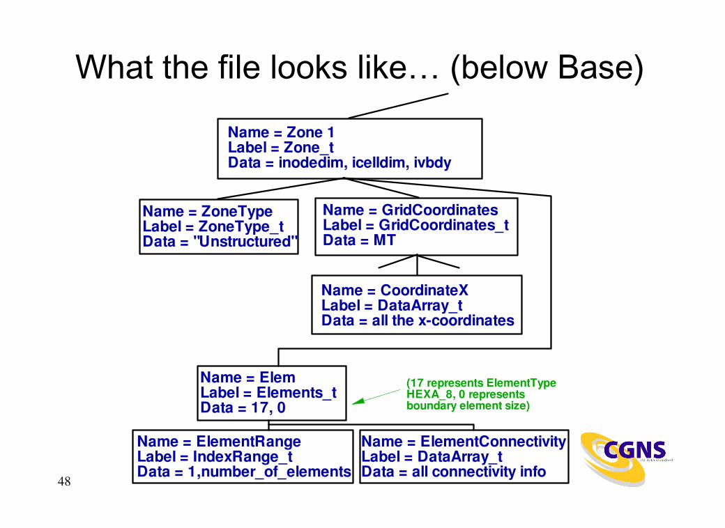
What the file looks like… (below Base)

Name = Zone 1Label = Zone_tData = inodedim, icelldim, ivbdy

Name = ElemLabel = Elements_tData = 17, 0

Name = GridCoordinatesLabel = GridCoordinates_tData = MT

Name = CoordinateXLabel = DataArray_tData = all the x-coordinates

Name = ElementConnectivityLabel = DataArray_tData = all connectivity info

Name = ZoneTypeLabel = ZoneType_tData = "Unstructured"

Name = ElementRangeLabel = IndexRange_tData = 1,number_of_elements

(17 represents ElementTypeHEXA_8, 0 representsboundary element size)

49

What the file looks like in adfviewer…