cgns standard interface data structures - higher...

DRAFT

-For

publ

icre

view

only

Mar

ch20

14AIAA R-101B-201X(Revision of AIAA R-101A-2005)

Recommended Practice

CFD General Notation System:Standard Interface Data Structures

Sponsored by

American Institute of Aeronautics and Astronautics

Approved

TBD

Abstract

The CFD General Notation System (CGNS) is a standard for recording and recovering computerdata associated with the numerical solution of the equations of fluid dynamics. The intent is tofacilitate the exchange of CFD data between sites, between applications codes, and across computingplatforms, and to s tabilize the archiving of CFD data. The CGNS system consists of a collectionof conventions, and software implementing those conventions, for the storage and retrieval of CFDdata. It consists of two parts: (1) a standard format for recording the data, and (2) software thatreads, writes, and modifies data in that format. The format is a conceptual entity established bythe documentation; the software is a physical product supplied to enable developers to access andproduce data recorded in that format. The standard format, or paper convention, part of CGNSconsists of two fundamental pieces. The first, known as the Standard Interface Data Structures, isdescribed in this Recommended Practice. It defines the intellectual content of the information tobe stored. The second, known as the File Mapping, defines the exact location in a CGNS file wherethe data is to be stored.

DRAFT

-For

publ

icre

view

only

Mar

ch20

14

AIAA R-101B-201X

Published by

American Institute of Aeronautics and Astronautics

1801 Alexander Bell Drive, Reston, VA 20191

Copyright c©201X American Institute of Aeronautics and Astronautics

All rights reserved

No part of this publication may be reproduced in any form, in an electronic retrieval system orotherwise, without prior written consent of the publisher.

Printed in the United States of America

ISBN 978-1-62410-269-1

ii

DRAFT

-For

publ

icre

view

only

Mar

ch20

14

AIAA R-101B-201X

Contents

Foreward 1

1 Introduction 31.1 Major Differences from Previous CGNS Versions . . . . . . . . . . . . . . . . . . . . 4

1.1.1 Version 3.2 . . . . . . . . . . . . . . . . . . . . . . . . . . . . . . . . . . . . . 51.1.2 Version 3.1 . . . . . . . . . . . . . . . . . . . . . . . . . . . . . . . . . . . . . 51.1.3 Version 2.5 . . . . . . . . . . . . . . . . . . . . . . . . . . . . . . . . . . . . . 61.1.4 Version 2.4 . . . . . . . . . . . . . . . . . . . . . . . . . . . . . . . . . . . . . 61.1.5 Version 2.3 . . . . . . . . . . . . . . . . . . . . . . . . . . . . . . . . . . . . . 61.1.6 Version 2.2, Beta 1 . . . . . . . . . . . . . . . . . . . . . . . . . . . . . . . . . 71.1.7 Version 2.1, Beta 1 . . . . . . . . . . . . . . . . . . . . . . . . . . . . . . . . . 71.1.8 Version 2.0, Beta 2 . . . . . . . . . . . . . . . . . . . . . . . . . . . . . . . . . 71.1.9 Version 2.0, Beta 1 . . . . . . . . . . . . . . . . . . . . . . . . . . . . . . . . . 8

2 Design Philosophy of Standard Interface Data Structures 9

3 Conventions 133.1 Data Structure Notation Conventions . . . . . . . . . . . . . . . . . . . . . . . . . . 133.2 Structured Grid Notation and Indexing Conventions . . . . . . . . . . . . . . . . . . 173.3 Unstructured Grid Element Numbering Conventions . . . . . . . . . . . . . . . . . . 18

3.3.1 1-D (Line) Elements . . . . . . . . . . . . . . . . . . . . . . . . . . . . . . . . 193.3.2 2-D (Surface) Elements . . . . . . . . . . . . . . . . . . . . . . . . . . . . . . 20

3.3.2.1 Triangular Elements . . . . . . . . . . . . . . . . . . . . . . . . . . . 203.3.2.2 Quadrilateral Elements . . . . . . . . . . . . . . . . . . . . . . . . . 22

3.3.3 3-D (Volume) Elements . . . . . . . . . . . . . . . . . . . . . . . . . . . . . . 233.3.3.1 Tetrahedral Elements . . . . . . . . . . . . . . . . . . . . . . . . . . 243.3.3.2 Pyramid Elements . . . . . . . . . . . . . . . . . . . . . . . . . . . . 263.3.3.3 Pentahedral Elements . . . . . . . . . . . . . . . . . . . . . . . . . . 293.3.3.4 Hexahedral Elements . . . . . . . . . . . . . . . . . . . . . . . . . . 32

3.3.4 Unstructured Grid Example . . . . . . . . . . . . . . . . . . . . . . . . . . . . 353.4 Multizone Interfaces . . . . . . . . . . . . . . . . . . . . . . . . . . . . . . . . . . . . 37

4 Building-Block Structure Definitions 414.1 Definition: DataClass_t . . . . . . . . . . . . . . . . . . . . . . . . . . . . . . . . . . 414.2 Definition: Descriptor_t . . . . . . . . . . . . . . . . . . . . . . . . . . . . . . . . . 414.3 Definition: DimensionalUnits_t . . . . . . . . . . . . . . . . . . . . . . . . . . . . . 424.4 Definition: DimensionalExponents_t . . . . . . . . . . . . . . . . . . . . . . . . . . 434.5 Definition: GridLocation_t . . . . . . . . . . . . . . . . . . . . . . . . . . . . . . . . 444.6 Definition: IndexArray_t . . . . . . . . . . . . . . . . . . . . . . . . . . . . . . . . . 444.7 Definition: IndexRange_t . . . . . . . . . . . . . . . . . . . . . . . . . . . . . . . . . 454.8 Definition: Rind_t . . . . . . . . . . . . . . . . . . . . . . . . . . . . . . . . . . . . . 45

5 Data-Array Structure Definitions 475.1 Definition: DataArray_t . . . . . . . . . . . . . . . . . . . . . . . . . . . . . . . . . . 47

iii

DRAFT

-For

publ

icre

view

only

Mar

ch20

14

AIAA R-101B-201X

5.1.1 Definition: DataConversion_t . . . . . . . . . . . . . . . . . . . . . . . . . . 485.2 Data Manipulation . . . . . . . . . . . . . . . . . . . . . . . . . . . . . . . . . . . . . 49

5.2.1 Dimensional Data . . . . . . . . . . . . . . . . . . . . . . . . . . . . . . . . . 495.2.2 Nondimensional Data Normalized by Dimensional Quantities . . . . . . . . . 505.2.3 Nondimensional Data Normalized by Unknown Dimensional Quantities . . . 505.2.4 Nondimensional Parameters . . . . . . . . . . . . . . . . . . . . . . . . . . . . 535.2.5 Dimensionless Constants . . . . . . . . . . . . . . . . . . . . . . . . . . . . . . 54

5.3 Data-Array Examples . . . . . . . . . . . . . . . . . . . . . . . . . . . . . . . . . . . 54

6 Hierarchical Structures 596.1 CGNS Version . . . . . . . . . . . . . . . . . . . . . . . . . . . . . . . . . . . . . . . 596.2 CGNS Entry Level Structure Definition: CGNSBase_t . . . . . . . . . . . . . . . . . . 596.3 Zone Structure Definition: Zone_t . . . . . . . . . . . . . . . . . . . . . . . . . . . . 626.4 Precedence Rules and Scope Within the Hierarchy . . . . . . . . . . . . . . . . . . . 66

7 Grid Coordinates, Elements, and Flow Solutions 697.1 Grid Coordinates Structure Definition: GridCoordinates_t . . . . . . . . . . . . . . 697.2 Grid Coordinates Examples . . . . . . . . . . . . . . . . . . . . . . . . . . . . . . . . 717.3 Elements Structure Definition: Elements_t . . . . . . . . . . . . . . . . . . . . . . . 747.4 Elements Examples . . . . . . . . . . . . . . . . . . . . . . . . . . . . . . . . . . . . . 777.5 Axisymmetry Structure Definition: Axisymmetry_t . . . . . . . . . . . . . . . . . . . 817.6 Rotating Coordinates Structure Definition: RotatingCoordinates_t . . . . . . . . . 827.7 Flow Solution Structure Definition: FlowSolution_t . . . . . . . . . . . . . . . . . . 837.8 Flow Solution Example . . . . . . . . . . . . . . . . . . . . . . . . . . . . . . . . . . 867.9 Zone Subregion Structure Definition: ZoneSubRegion_t . . . . . . . . . . . . . . . . 897.10 Zone Subregion Examples . . . . . . . . . . . . . . . . . . . . . . . . . . . . . . . . . 92

8 Multizone Interface Connectivity 958.1 Zonal Connectivity Structure Definition: ZoneGridConnectivity_t . . . . . . . . . 958.2 1-to-1 Interface Connectivity Structure Definition: GridConnectivity1to1_t . . . . 968.3 1-to-1 Interface Connectivity Examples . . . . . . . . . . . . . . . . . . . . . . . . . . 998.4 General Interface Connectivity Structure Definition: GridConnectivity_t . . . . . . 1018.5 General Interface Connectivity Examples . . . . . . . . . . . . . . . . . . . . . . . . 1088.6 Grid Connectivity Property Structure Definition: GridConnectivityProperty_t . . 111

8.6.1 Periodic Interface Structure Definition: Periodic_t . . . . . . . . . . . . . . 1118.6.2 Average Interface Structure Definition: AverageInterface_t . . . . . . . . . 112

8.7 Overset Grid Holes Structure Definition: OversetHoles_t . . . . . . . . . . . . . . . 113

9 Boundary Conditions 1159.1 Boundary Condition Structures Overview . . . . . . . . . . . . . . . . . . . . . . . . 1169.2 Zonal Boundary Condition Structure Definition: ZoneBC_t . . . . . . . . . . . . . . 1179.3 Boundary Condition Structure Definition: BC_t . . . . . . . . . . . . . . . . . . . . . 1199.4 Boundary Condition Data Set Structure Definition: BCDataSet_t . . . . . . . . . . . 1229.5 Boundary Condition Data Structure Definition: BCData_t . . . . . . . . . . . . . . . 1259.6 Boundary Condition Property Structure Definition: BCProperty_t . . . . . . . . . . 126

iv

DRAFT

-For

publ

icre

view

only

Mar

ch20

14

AIAA R-101B-201X

9.6.1 Wall Function Structure Definition: WallFunction_t . . . . . . . . . . . . . 1279.6.2 Area Structure Definition: Area_t . . . . . . . . . . . . . . . . . . . . . . . . 127

9.7 Boundary Condition Type Structure Definition: BCType_t . . . . . . . . . . . . . . . 1289.8 Matching Boundary Condition Data Sets . . . . . . . . . . . . . . . . . . . . . . . . 1329.9 Boundary Condition Specification Data . . . . . . . . . . . . . . . . . . . . . . . . . 1349.10 Boundary Condition Examples . . . . . . . . . . . . . . . . . . . . . . . . . . . . . . 136

10 Governing Flow Equations 14510.1 Flow Equation Set Structure Definition: FlowEquationSet_t . . . . . . . . . . . . . 14510.2 Governing Equations Structure Definition: GoverningEquations_t . . . . . . . . . . 14610.3 Model Type Structure Definition: ModelType_t . . . . . . . . . . . . . . . . . . . . 14810.4 Thermodynamic Gas Model Structure Definition: GasModel_t . . . . . . . . . . . . 14810.5 Molecular Viscosity Model Structure Definition: ViscosityModel_t . . . . . . . . . 15010.6 Thermal Conductivity Model Structure Definition: ThermalConductivityModel_t . 15210.7 Turbulence Structure Definitions . . . . . . . . . . . . . . . . . . . . . . . . . . . . . 154

10.7.1 Turbulence Closure Structure Definition: TurbulenceClosure_t . . . . . . . 15410.7.2 Turbulence Model Structure Definition: TurbulenceModel_t . . . . . . . . . 155

10.8 Thermal Relaxation Model Structure Definition: ThermalRelaxationModelType_t 15810.9 Chemical Kinetics Structure Definition: ChemicalKineticsModel_t . . . . . . . . . 15910.10Electromagnetics Structure Definitions . . . . . . . . . . . . . . . . . . . . . . . . . . 161

10.10.1 Electromagnetics Electric Field Model Structure Definition: EMElectric-FieldModel_t . . . . . . . . . . . . . . . . . . . . . . . . . . . . . . . . . . . 162

10.10.2 Electromagnetics Magnetic Field Model Structure Definition: EMMagnetic-FieldModel_t . . . . . . . . . . . . . . . . . . . . . . . . . . . . . . . . . . . 163

10.10.3 Electromagnetics Conductivity Model Structure Definition: EMConductivi-tyModel_t . . . . . . . . . . . . . . . . . . . . . . . . . . . . . . . . . . . . . 164

10.11Flow Equation Examples . . . . . . . . . . . . . . . . . . . . . . . . . . . . . . . . . 165

11 Time-Dependent Flow 16911.1 Iterative Data Structure Definitions . . . . . . . . . . . . . . . . . . . . . . . . . . . 169

11.1.1 Base Iterative Data Structure Definition: BaseIterativeData_t . . . . . . . 16911.1.2 Zone Iterative Data Structure Definition: ZoneIterativeData_t . . . . . . . 170

11.2 Rigid Grid Motion Structure Definition: RigidGridMotion_t . . . . . . . . . . . . . 17111.3 Arbitrary Grid Motion Structure Definition: ArbitraryGridMotion_t . . . . . . . . 17311.4 Zone Grid Connectivities . . . . . . . . . . . . . . . . . . . . . . . . . . . . . . . . . 17611.5 Examples for Time-Dependent Flow . . . . . . . . . . . . . . . . . . . . . . . . . . . 176

12 Miscellaneous Data Structures 18312.1 Reference State Structure Definition: ReferenceState_t . . . . . . . . . . . . . . . 18312.2 Reference State Example . . . . . . . . . . . . . . . . . . . . . . . . . . . . . . . . . 18412.3 Convergence History Structure Definition: ConvergenceHistory_t . . . . . . . . . . 18512.4 Discrete Data Structure Definition: DiscreteData_t . . . . . . . . . . . . . . . . . . 18712.5 Integral Data Structure Definition: IntegralData_t . . . . . . . . . . . . . . . . . . 18912.6 Family Data Structure Definition: Family_t . . . . . . . . . . . . . . . . . . . . . . . 19012.7 Geometry Reference Structure Definition: GeometryReference_t . . . . . . . . . . . 192

v

DRAFT

-For

publ

icre

view

only

Mar

ch20

14

AIAA R-101B-201X

12.8 Family Boundary Condition Structure Definition: FamilyBC_t . . . . . . . . . . . . 19312.9 Family Boundary Condition Data Set Structure Definition: FamilyBCDataSet_t . . 19412.10User-Defined Data Structure Definition: UserDefinedData_t . . . . . . . . . . . . . 19512.11Gravity Data Structure Definition: Gravity_t . . . . . . . . . . . . . . . . . . . . . 196

A Conventions for Data-Name Identifiers 199A.1 Coordinate Systems . . . . . . . . . . . . . . . . . . . . . . . . . . . . . . . . . . . . 199A.2 Flowfield Solution . . . . . . . . . . . . . . . . . . . . . . . . . . . . . . . . . . . . . 200A.3 Turbulence Model Solution . . . . . . . . . . . . . . . . . . . . . . . . . . . . . . . . 208A.4 Nondimensional Parameters . . . . . . . . . . . . . . . . . . . . . . . . . . . . . . . . 208A.5 Characteristics and Riemann Invariants Based on 1-D Flow . . . . . . . . . . . . . . 210A.6 Forces and Moments . . . . . . . . . . . . . . . . . . . . . . . . . . . . . . . . . . . . 210A.7 Time-Dependent Flow . . . . . . . . . . . . . . . . . . . . . . . . . . . . . . . . . . . 213

B Structured Two-Zone Flat Plate Example 215B.1 Overall Layout . . . . . . . . . . . . . . . . . . . . . . . . . . . . . . . . . . . . . . . 215B.2 Grid Coordinates . . . . . . . . . . . . . . . . . . . . . . . . . . . . . . . . . . . . . . 217B.3 Flowfield Solution . . . . . . . . . . . . . . . . . . . . . . . . . . . . . . . . . . . . . 218B.4 Interface Connectivity . . . . . . . . . . . . . . . . . . . . . . . . . . . . . . . . . . . 220B.5 Boundary Conditions . . . . . . . . . . . . . . . . . . . . . . . . . . . . . . . . . . . . 223B.6 Global Reference State . . . . . . . . . . . . . . . . . . . . . . . . . . . . . . . . . . . 226B.7 Equation Description . . . . . . . . . . . . . . . . . . . . . . . . . . . . . . . . . . . . 228

List of Figures

1 Sample Topologically Based CFD Hierarchy . . . . . . . . . . . . . . . . . . . . . . . 102 Structured-Grid Multizone Interface Types . . . . . . . . . . . . . . . . . . . . . . . 383 Example Tetrahedral Grid . . . . . . . . . . . . . . . . . . . . . . . . . . . . . . . . . 784 Example Interface for 1-to-1 Connectivity . . . . . . . . . . . . . . . . . . . . . . . . 1005 Example Interface for Generalized Connectivity, Structured Grids . . . . . . . . . . . 1086 Example Interface for Generalized Connectivity, Unstructured Grids with HEXA_8

Donor Cell . . . . . . . . . . . . . . . . . . . . . . . . . . . . . . . . . . . . . . . . . 1107 Example Interface for Generalized Connectivity, Unstructured Grids with TRI_3

Donor Cell . . . . . . . . . . . . . . . . . . . . . . . . . . . . . . . . . . . . . . . . . 1108 Hierarchy for Boundary Condition Structures . . . . . . . . . . . . . . . . . . . . . . 1179 Boundary Condition Implementation Levels . . . . . . . . . . . . . . . . . . . . . . . 13610 Two-Zone Flat Plate Test Case . . . . . . . . . . . . . . . . . . . . . . . . . . . . . . 215

List of Tables

1 Element Types in CGNS . . . . . . . . . . . . . . . . . . . . . . . . . . . . . . . . . . 192 Simple Boundary Condition Types . . . . . . . . . . . . . . . . . . . . . . . . . . . . 1293 Compound Boundary Condition Types . . . . . . . . . . . . . . . . . . . . . . . . . . 1324 Associated Boundary Condition Types and Usage Rules . . . . . . . . . . . . . . . . 1335 Data-Name Identifiers for Perfect Gas . . . . . . . . . . . . . . . . . . . . . . . . . . 150

vi

DRAFT

-For

publ

icre

view

only

Mar

ch20

14

AIAA R-101B-201X

6 Data-Name Identifiers for Molecular Viscosity Models . . . . . . . . . . . . . . . . . 1517 Data-Name Identifiers for Thermal Conductivity Models . . . . . . . . . . . . . . . . 1538 Data-Name Identifiers for Turbulence Closure . . . . . . . . . . . . . . . . . . . . . . 1559 Data-Name Identifiers for Chemical Kinetics Models . . . . . . . . . . . . . . . . . . 16010 Defined Names (Symbols) for Commonly Used Mixtures . . . . . . . . . . . . . . . . 16111 Data-Name Identifiers for Electromagnetics Models . . . . . . . . . . . . . . . . . . . 16512 Data-Name Identifiers for Rigid Grid Motion . . . . . . . . . . . . . . . . . . . . . . 17313 Data-Name Identifiers for Grid Velocity . . . . . . . . . . . . . . . . . . . . . . . . . 17514 Data-Name Identifiers for Reference State . . . . . . . . . . . . . . . . . . . . . . . . 18415 Data-Name Identifiers for Coordinate Systems . . . . . . . . . . . . . . . . . . . . . . 20016 Data-Name Identifiers for Flow Solution Quantities . . . . . . . . . . . . . . . . . . . 20217 Data-Name Identifiers for Typical Turbulence Models . . . . . . . . . . . . . . . . . 20818 Data-Name Identifiers for Nondimensional Parameters . . . . . . . . . . . . . . . . . 20919 Data-Name Identifiers for Characteristics and Riemann Invariants . . . . . . . . . . 21020 Data-Name Identifiers for Forces and Moments . . . . . . . . . . . . . . . . . . . . . 21221 Data-Name Identifiers for Time-Dependent Flow . . . . . . . . . . . . . . . . . . . . 213

vii

DRAFT

-For

publ

icre

view

only

Mar

ch20

14

DRAFT

-For

publ

icre

view

only

Mar

ch20

14

AIAA R-101B-201X

Foreward

This document contains the Standard Interface Data Structures (SIDS) definitions for the CFDGeneral Notation System (CGNS) project; this project was originally a NASA-funded contractunder the AST program, but control has now been completely transferred to a public forum knownas the CGNS Steering Committee. This document corresponds to the online SIDS DocumentVersion 3.2.4.

The purpose of this document is to scope the information that should be communicated betweenvarious CFD application codes; the target is 3–D multizone, compressible Navier-Stokes analysis.Attention in this document is not focussed on I/O routines or formats, but on the precise descriptionof data that should be present in the I/O of a CFD code or in a CFD database.

This document therefore contains a precise definition of information pertinent to a CGNS database.Specifically, the following information is addressed:

• grid coordinates and elements

• flow solution data, including nondimensional parameters

• multizone interface connectivity, including abutting and overset

• boundary conditions

• flow equation descriptions

• time-dependent flow

• reference states

• dimensional units and nondimensionalization information associated with data

• convergence history

• association to geometry definition

• topologically based hierarchical structures

Information is encoded into C-like data structures.

This document replaces (in whole) earlier versions. Major changes made to the document since itslast release are outlined in Section 1.1.

At the time of approval, the approving subcommittee of members of the CGNS Steering Committeecomprised the following individuals:

Thomas Hauser, Chair University of Colorado at Boulder

Juan Alonso Stanford University

Pat Baker Pointwise, Inc.

1

DRAFT

-For

publ

icre

view

only

Mar

ch20

14

AIAA R-101B-201X

Bob Bush Pratt & Whitney

Stephen Guzik Colorado State University

Richard Hann ANSYS/CFX

Anthony Iannetti NASA Glenn

Scott Imlay Tecplot, Inc.

Xiangmin (Jim) Jiao Stony Brook University

Simon Pereira ANSYS/ICEM CFD

Marc Poinot ONERA

Chris Rumsey NASA Langley

ZJ Wang University of Kansas

Brad Whitlock Intelligent Light

The above consensus body approved this document in Month Year.

The AIAA Standards Executive Council (VP-Standards Name, Chairperson) accepted the docu-ment for publication in Month Year.

The AIAA Standards Procedures dictates that all approved standards, recommended practices,and guides are advisory only. Their use by anyone engaged in industry or trade is entirely volun-tary. There is no agreement to adhere to any AIAA standards publication and no commitment toconform to or be guided by standards reports. In formulating, revising, and approving standardspublications, the committees on standards will not consider patents that may apply to the subjectmatter. Prospective users of the publications are responsible for protecting themselves againstliability for infringement of patents or copyright, or both.

2

DRAFT

-For

publ

icre

view

only

Mar

ch20

14

AIAA R-101B-201X

1 Introduction

CGNS (CFD General Notation System) is a collection of conventions, along with software imple-menting those conventions, for the storage and retrieval of CFD (computational fluid dynamics)data. The CGNS system is designed to facilitate the exchange of data between sites and appli-cations, as well as to help stabilize the archiving of fluid dynamic data. In today’s environment,it is important in many technical arenas to maintain detailed records of scientific computations.CGNS was designed to help promote a long-lasting and extensible standard for this purpose. Manycompanies and institutions choose to adopt the CGNS standard in order to increase productivity by(1) reducing the time required to translate between data created and used by different applications,and (2) increasing the quality, longevity, and re-usability of archived data.

The CGNS standard is a conceptual entity established by the documentation. The CGNS softwareis a physical product supplied to enable writing and reading data according to this standard. AllCGNS software is completely free and open to anyone. By using the supplied software, it is relativelyeasy for users to adhere to most of the standard described in detail in this document.

The CGNS project originated during 1994 through a series of meetings that addressed improvedtransfer of NASA technology to industry. A principal impediment in this process was the disparityin I/O formats employed by various flow codes, grid generators, and other utilities, and CGNSwas conceived as a means to promote “plug-and-play” CFD. An agreement was reached to developCGNS at Boeing, under NASA Contract NAS1-20267, with active participation by a team of CFDresearchers from NASA’s Langley, Lewis (now Glenn), and Ames Research Centers, McDonnellDouglas Corporation (now part of Boeing), and Boeing Commercial Airplane Group. This team,which was joined by ICEM CFD Engineering Corporation of Berkeley, California in 1997, undertookthe core of the development. However, in the spirit of creating a completely open and broadlyaccepted standard, all interested parties were encouraged to participate; the US Air Force andArnold Engineering Development Center were notably present. From the beginning, the purposewas to develop a system that could be distributed freely, including all documentation, software andsource code. This goal has now been fully realized; further, control of CGNS has been completelytransferred to a public forum known as the CGNS Steering Committee.

The principal target is the data normally associated with compressible viscous flow (i.e., the Navier-Stokes equations), but the standard is also applicable to subclasses such as Euler and potential flows.The initial release addressed multi-zone grids, flow fields, boundary conditions, and zone-to-zoneconnection information, as well as a number of auxiliary items, such as non-dimensionalization,reference states, and equation set specifications. Extensions incorporated since then include un-structured mesh, connections to geometry definition, time-dependent flow, and support for multiplespecies and chemistry.

It is worth noting that extensibility is a fundamental design characteristic of the system, whichin principal could be used for other disciplines of computational field physics, such as acoustics orelectromagnetics, given the willingness of the cognizant scientific community to define the conven-tions.

The standard format, or paper convention, part of CGNS consists of two fundamental pieces. Thefirst, known as the Standard Interface Data Structures (SIDS), describes in detail the intellectualcontent of the information to be stored. It defines, for example, the precise meaning of a “boundary

3

DRAFT

-For

publ

icre

view

only

Mar

ch20

14

AIAA R-101B-201X

condition”. The second, known as the SIDS File Mapping defines the exact location in a CGNS filewhere the data is to be stored.

The implementation, or software, part of CGNS likewise consists of two separate entities. CGNSfiles are read and written by a stand-alone database manager, either ADF (Advanced Data Format)or HDF (Hierarchical Data Format). The database manager implements a tree-like data structure,as a binary file. Since the format of this file is completely controlled by the database manager, andsince ADF and HDF are both written in ANSI C (Fortran wrappers are provided), these files andthe database manager itself are portable to any environment that supports ANSI C. Both ADFand HDF are available separately and constitute useful tools for the storage of large quantities ofscientific data.

The underlying database manager, however, implements no knowledge of CFD or of the File Map-ping. To simplify access to CGNS files, a second layer of software known as the Mid-Level Libraryis provided. This layer is in effect an API, or Application Programming Interface for CFD. The APIincorporates knowledge of the CFD data structures, their meaning and their location in the file,enabling applications such as flow codes and grid generators to access the data in familiar terms.The API is therefore the piece of the CGNS system most visible to applications developers. Likethe ADF and HDF database managers, the Mid-Level Library is written in ANSI C; all public APIroutines have Fortran counterparts.

This document presents the formal definition of the Standard Interface Data Structures (SIDS).Section 2 presents the major design philosophies used to develop the CGNS database and theencoding of this database into the SIDS; this section also provides an overview of the databasehierarchy. Section 3 describes the C-like nomenclature conventions used to define the SIDS. Thissection also gives the conventions for structured grid indexing and unstructured element numbering,and the nomenclature for multizone interfaces. Low-level building-block structures are defined inSection 4; these structures are used to define all higher-level structures. Structures for defining dataarrays, including dimensional-units and nondimensional information, are presented in Section 5.The top levels of the CGNS hierarchy are next defined in Section 6. The following sections thenfill out the remainder of the hierarchy: Section 7 defines the grid-coordinate, elements, and flow-solution structures; Section 8 defines the multizone interface connectivity structures; Section 9defines boundary-condition structures; Section 10 defines structures for describing governing flowequations; Section 11 defines structures related to time-dependent flows; and Section 12 containsmiscellaneous structures. Two appendices complete the document. Appendix A provides namingconventions for data contained within the CGNS database, and Appendix B contains a completeSIDS description of a structured-grid two-zone test case.

1.1 Major Differences from Previous CGNS Versions

The following items represent noteworthy alterations and additions to the SIDS in reverse chrono-logical order. References to CPEX in the following refer to CGNS Proposals for Extension.1

1CPEX descriptions can be found at http://cgns.sourceforge.net/Proposals.html; last accessed 7/26/2013.

4

DRAFT

-For

publ

icre

view

only

Mar

ch20

14

AIAA R-101B-201X

1.1.1 Version 3.2

The following changes were made for Version 3.2

• Added AdditionalFamilyName t under BC t (Section 9.3), Zone t (Section 6.3), ZoneSubRe-gion t (Section 7.9), and UserDefinedData t (Section 12.10); and added FamilyName t underFamily t (Section 12.6) (a hierarchy of families is now possible); according to CPEX 0033 and0034.

• Added new cubic elements in Section 3.3, according to CPEX 0036.

1.1.2 Version 3.1

The following changes were made for Version 3.1

• Added a PYRA_13 element in the description of the unstructured grid element numberingconventions for pyramid elements (Section 3.3.3).

• Modified the description of the Elements_t structure to incorporate the new definition of theNGON_n element type, and added the NFACE_n element type. Also added examples illustratingtheir use, including for polyhedral elements (Section 7.3).

• References to Null were changed to xxxxNull, and references to UserDefined were changedto xxxxUserDefined, as appropriate. Also made sure that the xxxxNull is listed first, andthe xxxxUserDefined is listed second.

• Added section Model Type Structure Definition (Section 10.3).

• Added ZoneSubRegion_t (CPEX 0030) (Section 7.9). Made changes associated with CPEX0031: (1) added CellDimension to several places in Zone_t, (2) added new ParentElementsand ParentElementsPosition in Elements_t, (3) added CellDimension and revamped usageof PointList and PointRange in FlowSolution_t, (4) added CellDimension to several placesin ZoneBC_t, (5) added CellDimension and revamped usage of PointList and PointRange inBC_t, (6) changes in BCDataSet_t, (7) added CellDimension and revamped usage of PointListand PointRange in DiscreteData_t, (8) changes in FamilyBC_t, (9) creation of new Fam-ilyBCDataSet_t, (10) changes in Zone Grid Connectivities, and (11) addition of ZoneGrid-ConnectivityPointers and ZoneSubRegionPointers in ZoneIterativeData_t. A note re-garding CPEX 0031: The use of ElementList and ElementRange has been deprecated infavor of PointList and PointRange, as described in CPEX 0031 and in relevant sections ofthis document.

• Added clarity that if rotating about more than 1 axis, then it is done in a particular order inPeriodic_t and in Data-Name Identifiers for Rigid Grid Motion. (Table 12)

• Modified table in Section 9.3 to include CellCenter GridLocation.

5

DRAFT

-For

publ

icre

view

only

Mar

ch20

14

AIAA R-101B-201X

1.1.3 Version 2.5

No changes were made to the data structures for Version 2.5.

1.1.4 Version 2.4

The following changes were made for Version 2.4.

• GridLocation_t, PointRange, and PointList have been added to the BCDataSet_t datastructure, allowing boundary conditions to be specified at locations different from those usedto defined the BC patch. (E.g., a BC patch may be defined using vertices, with boundaryconditions applied at face centers.) (Section 9.4).

• Data structures have been added to FlowEquationSet_t for describing the electric field,magnetic field, and conductivity models used for electromagnetic flows. Corresponding rec-ommended data-name identifiers have also been added. (Section 10.1 and Section 10.10).

• RotatingCoordinates_t has been added to the Family_t data structure. (Section 12.6).

• A BCDataSet_t list has been added to the FamilyBC_t data structure, allowing specificationof boundary condition data arrays for CFD families. (Section 12.8).

• GridLocation_t, PointRange, PointList, FamilyName_t, UserDefinedData_t, and Ordi-nal have been added to the UserDefinedData_t data structure. (Section 12.10).

• The DimensionalUnits_t and DimensionalExponents_t structures have been expanded toinclude units for electric current, substance amount, and luminous intensity. (Section 4.3).

• The capability to include rind data with unstructured grids has been added, and Rind_t hasbeen added to the Elements_t structure, allowing specification of connectivity informationfor rind elements. (Section 4.8).

1.1.5 Version 2.3

The following changes were made for Version 2.3.

• ElementRange and ElementList have been added to the BC_t data structure. ElementRangeor ElementList may now be used to define a boundary condition patch by specifying faceindices, instead of using PointRange or PointList with GridLocation set to FaceCenter.The use of PointRange or PointList to define a boundary condition patch hasn’t changed.They may be used to define a boundary condition patch by specifying either vertex or faceindices.

When PointRange or PointList is used, the choice between vertex or face indices is de-termined by the value of GridLocation_t. When ElementRange or ElementList is used,GridLocation_t is ignored (Section 9.3).

6

DRAFT

-For

publ

icre

view

only

Mar

ch20

14

AIAA R-101B-201X

1.1.6 Version 2.2, Beta 1

The following changes were made for Version 2.2, Beta 1.

• Axisymmetry_t and RotatingCoordinates_t nodes have been added, allowing the recordingof data relevant to axisymmetric flows and rotating coordinates (Section 7.5 and Section 7.6).

• A Gravity_t node has been added for storage of the gravitational vector (Section 12.11).

• A GridConnectivityProperty_t node has been added, allowing the recording of specialproperties associated with particular connectivity patches, such as periodic interfaces, orinterfaces where the data is to be averaged in some way prior to passing it to a neighboringinterface (Section 8.6).

• A BCProperty_t node has been added, allowing the recording of special properties asso-ciated with particular boundary condition patches, such as wall function or bleed regions(Section 9.6).

• Additional flow solution data-name identifiers are included for variables in rotating coordinatesystems (Appendix A.2).



• A node type UserDefinedData_t (Section 12.10) is added for the storage of arbitrary userdefined data in Descriptor_t and DataArray_t children without the restrictions or implicitmeanings imposed on these node types at other node locations.

• Support for multi-species flows and chemistry has been added. New gas models have beenadded to the GasModelType_t enumeration (Section 10.4), and ThermalRelaxationModel_tand ChemicalKineticsModel_t data structures have been added for describing the thermalrelaxation and chemical kinetics models (Section 10.8 and Section 10.9). Additional flowsolution data-name identifiers are included (Appendix A.2).



• The following data structures related to time-dependent flow have been added: BaseIter-ativeData_t (Section 11.1.1), ZoneIterativeData_t (Section 11.1.2), RigidGridMotion_t(Section 11.2), ArbitraryGridMotion_t (Section 11.3).

7

DRAFT

-For

publ

icre

view

only

Mar

ch20

14

AIAA R-101B-201X



• The capability for recording unstructured zones has been added to the SIDS. (These changesoccur throughout the document, although some specific items are listed below.)

• The values UserDefined and Null are now allowed for all enumeration types (throughoutdocument).

• The following nodes are now defined (some of these also include additional new children sub-nodes): Family_t (Section 12.6), Elements_t (Section 7.3), ZoneType_t (Section 6.3), Fam-ilyName_t (Section 6.3), GeometryReference_t (Section 12.7), FamilyBC_t (Section 12.8).

• Under CGNSBase_t, the IndexDimension is no longer recorded; it has been replaced byCellDimension and PhysicalDimension (Section 6.2).

• Under Zone_t, the optional parameter VertexSizeBoundary has been added for unstructuredzones (Section 6.3).

• The method for general connectivity (GridConnectivity_t) has been altered. It now requiresthe use of either (a) PointListDonor (an integer, for Abutting1to1 only) or (b) CellList-Donor (an integer) plus InterpolantsDonor (a real) (Section 8.4).

• The GridLocation_t parameter has been moved up one level (from BCDataSet_t to BC_t).Thus, for example, if the boundary conditions are defined at vertices (the default), then anyassociated dataset information must also be specified at vertices (Section 9.3 and Section 9.4).

• The data-name identifier LengthReference has been added (Section 12.1 and Appendix A.2).

• The νt parameter has been renamed ViscosityEddyKinematic, and a new parameter Vis-cosityEddy, representing µt, has been defined (Appendix A.2).

8

DRAFT

-For

publ

icre

view

only

Mar

ch20

14

AIAA R-101B-201X

2 Design Philosophy of Standard Interface Data Structures

The major design goal of the SIDS is a comprehensive and unambiguous description of the “intel-lectual content” of information that must be passed from code to code in a multizone Navier-Stokesanalysis system. This information includes grids, flow solutions, multizone interface connectivity,boundary conditions, reference states and dimensional units or normalization associated with data.

Implications of CFD Data Sets

The goal is description of the data sets typical of CFD analysis, which tend to contain a smallnumber of extremely large data arrays. This has a number of implications for both the design ofthe SIDS and the ultimate physical files where the data resides. The first is that any I/O systembuilt for CFD analysis must be designed to efficiently store and process large data arrays. This isreflected in the SIDS, which includes provisions for describing large data arrays.

The second implication is that the nature of the data sets allows for thorough description of thedata with relatively little storage overhead and performance penalty. For example, the flow solutionof a CFD analysis may contain several millions of quantities. Therefore, with little penalty it ispossible to include information describing the flow variables stored, their location in the grid, anddimensional units or nondimensionalization associated with the data. The SIDS take advantage ofthis situation and includes an extensive description of the information stored in the database.

The third implication of CFD data sets is that files containing a CFD database are almost alwaysrequired to be binary – ASCII storage of CFD data involves excessive storage and performancepenalties. This means the files are not readable by humans and the information contained in themis not directly modifiable by text editors and such. This is reflected in the syntax of the SIDS,which tends to be verbose and thorough; whereas, directly modifiable ASCII file formats wouldtend to foster a more brief syntax.

It is important to note that the description of information by the SIDS is independent of physicalfile formats. However, it is targeted toward implementation using the ADF Core library. Some ofthe language components used to define the SIDS are meant to directly map into elements of anADF node.

Topologically Based Hierarchical Database

An early decision in the CGNS project was that any new CFD I/O standard should include ahierarchical database, such as a tree or directed graph. The SIDS describe a hierarchical database,precisely defining both the data and their hierarchical relationships.

There are two major alternatives to organizing a CFD hierarchy: topologically based and data-typebased. In a topologically based graph, overall organization is by zones; information pertaining to aparticular zone, including its grid coordinates or flow solution, hangs off the zone. In a data-typebased graph, organization is by related data. For example, there would be two nodes at the samelevel, one for grid coordinates and another for the flow solution. Hanging off each of these nodeswould be separate lists of the zones.

9

DRAFT

-For

publ

icre

view

only

Mar

ch20

14

AIAA R-101B-201X

CGNS databaser��rReference state

""

"""

"""rrZone 1

!!!!!!!!!!!rrGrid coordinates

x y z

@@@@@

��

��r r r

aaaaaaaaaaarrFlow solution

ρ ρu ρv ρw ρe0

@@@@@

��

��

HHHHHHHHH

��r r r r r

rr

Multizone interfaceconnectivity

��@@

````````````````````` rrBoundary conditions

��@@

BBBBBrrZone 2

!!! aaa```

XXXXXXXXXXXXXXXXXXrrZone N

!!! aaa```

· · ·

Figure 1: Sample Topologically Based CFD Hierarchy

The hierarchy described in this document is topologically based; a simplified illustration of thedatabase hierarchy is shown in Figure 1. Hanging off the root “node” of the database is a nodecontaining global reference-state information, such as freestream conditions, and a list of nodes foreach zone. The figure shows the nodes that hang off the first zone; similar nodes would hang offof each zone in the database. Nodes containing the physical-coordinate data arrays (x, y and z)for the first zone are shown hanging off the “grid coordinates” node. Likewise, nodes containingthe first zone’s flow-solution data arrays hang off the “flow solution” node. The figure also depictsnodes containing multizone interface connectivity and boundary condition information for the firstzone; subnodes hanging off each of these are not pictured.

Additional Design Objectives

The data structures comprising the SIDS are the result of several additional design objectives:

One objective is to minimize duplication of data within the hierarchy. Many parameters, such as thegrid size of a zone, are defined in only one location. This avoids implementation problems arisingfrom data duplication within the physical file containing the database; these problems includesimultaneous update of all copies and error checking when two copies of a data quantity are foundto be different. One consequence of minimizing data duplication is that information at lower levelsof the hierarchy may not be completely decipherable without access to information at higher levels.For example, the grid size is defined in the zone structure (see Section 6.3), but this parameter isneeded in several substructures to define the size of grid and flow-solution data arrays. Therefore,these substructures are not autonomous and deciphering information within them requires access toinformation contained in the zone structure itself. The SIDS must reflect this cascade of informationwithin the database.

10

DRAFT

-For

publ

icre

view

only

Mar

ch20

14

AIAA R-101B-201X

Another objective is elimination of nonsensical descriptions of the data. The SIDS have beencarefully developed to avoid data qualifiers and other optional descriptive information that could beinconsistent. This has led to the use of specialized structures for certain CFD-related information.One example is a single-purpose structure for defining physical grid coordinates of a zone. It ispossible to define the grid coordinates, flow solution and any other field quantities within a zone by ageneric discrete-data structure. However, this requires the generic structure to include informationdefining the grid location of the data (e.g., the data is located at vertices or cell centers). Using thegeneric structure to describe the grid coordinates leads to a possible inconsistency. By definition thephysical coordinates that define the grid are located at vertices, and including an optional qualifierthat states otherwise makes no sense.

A final objective is to allow documentation inclusion throughout the database. The SIDS containa uniform documentation mechanism for all major structures in the hierarchy. However, thisdocument establishes no conventions for using the documentation mechanism.

11

DRAFT

-For

publ

icre

view

only

Mar

ch20

14

DRAFT

-For

publ

icre

view

only

Mar

ch20

14

AIAA R-101B-201X

3 Conventions

3.1 Data Structure Notation Conventions

The intellectual content of the CGNS database is defined in terms of C-like notation includingtypedefs and structures. The database is made up of entities, and each entity has a type associatedwith it. Entities include such things as the dimensionality of the grid, an array of grid coordinates,or a zone that contains all the data associated with a given region. Entities are defined in termsof types, where a type can be an integer or a collection of elements (a structure) or a hierarchy ofstructures or other similar constructs.

The terminology “instance of an entity” is used to refer to an entity that has been assigned a valueor whose elements have been assigned values. The terminology “specific instance of a structure” isalso used in the following sections. It is short for an instance of an entity whose type is a structure.

Names of entities and types are constructed using conventions typical of Mathematica.2 Names oridentifiers contain no spaces and capitalization is used to distinguish individual words making upa name; names are case-sensitive. The characters “.” and “/” should be avoided in names as thesehave special meaning when referencing elements of a structure entity.

The following notational conventions are employed:

! comment to end of line_t suffix used for naming a type; end of a definition, declaration, assignment or entity instance= assignment (takes on the value of):= indicates a type definition (typedef)[ ] delimiters of an array{ } delimiters of a structure definition{{ }} delimiters of an instance of a structure entity< > delimiters of a structure parameter listint integerreal floating-point numberchar characterbit bitEnumeration( ) indicates an enumeration typeData( ) indicates an array of data, which may be multidimensionalList( ) indicates a list of entitiesIdentifier( ) indicates an entity identifierLogicalLink( ) indicates a logical link/ delimiter for element of a structure entity../ delimiter for parent of a structure entity(r) designation for a required structure element(o) designation for an optional structure element(o/d) designation for an optional structure element with default if absent

2Mathematica 3.0, Wolfram Research, Inc., Champaign, IL (1996)

13

DRAFT-Forpublic

review

only

March2014AIAA R-101B-201X

An enumeration type is a set of values identified by names; names of values within a given enumer-ation declaration must be unique. An example of an enumeration type is the following:

Enumeration( Dog, Cat, Bird, Frog )

This defines an enumeration type which contains four values.

Data() identifies an array of given dimensionality and size in each dimension, whose elements areall of a given data type. It is written as,

Data( DataType, Dimension, DimensionValues[] ) ;

Dimension is an integer, and DimensionValues[] is an array of integers of size Dimension. Dimen-sion and DimensionValues[] specify the dimensionality of the array and its size in each dimension.DataType specifies the data type of the array’s elements; it may consist of one of the following:int, real, char or bit. For multidimensional arrays, FORTRAN indexing conventions are used.Data() is formulated to map directly onto the data section of an ADF node.

A typedef establishes a new type and defines it in terms of previously defined types. Types areidentified by the suffix “_t”, and the symbol “:=” is used to establish a type definition (or typedef).For example, the above enumeration example can be used in a typedef:

Pet_t := Enumeration( Dog, Cat, Bird, Frog ) ;

This defines a new type Pet_t, which can then be used to declare a new entity, such as,

Pet_t MyFavoritePet ;

By the above typedef and declaration, MyFavoritePet is an entity of type Pet_t and can have thevalues Dog, Cat, Bird or Frog. A specific instance of MyFavoritePet is setting it equal to one ofthese values (e.g., MyFavoritePet = Bird).

A structure is a type that can contain any number of elements, including elements that are alsostructures. An example of a structure type definition is:

Sample_t :={int Dimension ; (r)

real[4] Vector ; (o)

Pet_t ObnoxiousPet ; (o)} ;

where Sample_t is the type of the structure. This structure contains three elements, Dimension,Vector and ObnoxiousPet, whose types are int, real[4] and Pet_t, respectively. The type intspecifies an integer, and real[4] specifies an array of reals that is one-dimensional with a lengthof four. The “(r)” and “(o)” notation in the right margin is explained below. Given the definitionof Sample_t, entities of this type can then be declared (e.g., Sample_t Sample1;). An example ofan instance of a structure entity is given by,

14

DRAFT

-For

publ

icre

view

only

Mar

ch20

14

AIAA R-101B-201X

Sample_t Sample1 ={{Dimension = 3 ;Vector = [1.0, 3.45, 2.1, 5.4] ;ObnoxiousPet = Dog ;}} ;

Note the different functions played by single braces “{” and double braces “{{”. The first is usedto delimit the definition of a structure type; the second is used to delimit a specific instance of astructure entity.

Some structure type definitions contain arbitrarily long lists of other structures or types. Theselists will be identified by the notation,

List( Sample_t Sample1 ... SampleN ) ;

where Sample1 ... SampleN is the list of structure names or identifiers, each of which has the typeSample_t. Within each list, the individual structure names are user-defined.

In the CGNS database it is sometimes necessary to reference the name or identifier of a structureentity. References to entities are denoted by Identifier(), whose single argument is a structuretype. For example,

Identifier(Sample_t) SampleName ;

declares an entity, SampleName, whose value is the identifier of a structure entity of type Sample_t.Given this declaration, SampleName could be assigned the value Sample1 (i.e., SampleName =Sample1).

It is sometimes convenient to directly identify an element of a specific structure entity. It is alsoconvenient to indicate that two entities with different names are actually the same entity. Weborrow UNIX conventions to indicate both these features, and make the analogy that a structureentity is a UNIX directory and its elements are UNIX files. An element of an entity is designatedby “/”; an example is Sample1/Vector). The structure entity that a given element belongs to isdesignated “../” A UNIX-like logical link that specifies the sameness of two apparently differententities is identified by LogicalLink(); it has one argument. An example of a logical link is asfollows: Suppose a specific instance of a structure entity contains two elements that are of typeSample_t; call them SampleA and SampleB. The statement that SampleB is actually the same entityas SampleA is,

SampleB = LogicalLink(../SampleA) ;

The argument of LogicalLink() is the UNIX-like “path name” of the entity with which the link ismade. In this document, LogicalLink() and the direct specification of a structure element via “/”and “../” are actually seldom used. These language elements are never used in the actual definitionof a structure type.

15

DRAFT

-For

publ

icre

view

only

Mar

ch20

14

AIAA R-101B-201X

Structure type definitions include three additional syntactic/semantic notions. These are parame-terized structures, structure-related functions, and the identification of required and optional fieldswithin a structure.

As previously stated, one of our design objectives is to minimize duplication of information withinthe CGNS database. To meet this objective, information is often stored in only one location of thehierarchy; however, that information is typically used in other parts of the hierarchy. A consequenceof this is that it may not be possible to decipher all the information associated with a given entityin the hierarchy without knowledge of data contained in higher level entities. For example, thegrid size of a zone is stored in one location (in Zone_t, see Section 6.3), but is needed in manysubstructures to define the size of grid and solution-data arrays.

This organization of information must be reflected in the language used to describe the database.First, parameterized structures are introduced to formalize the notion that information must bepassed down the hierarchy. A given structure type is defined in terms of a list of parameters thatprecisely specify what information must be obtained from the structure’s parent. These structure-defining parameters play a similar role to subroutine parameters in C or FORTRAN and are used todefine fields within the structure; they are also passed onto substructures. Parameterized structuresare also loosely tied to templates in C++.

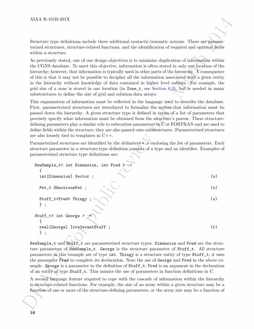
Parameterized structures are identified by the delimiters < > enclosing the list of parameters. Eachstructure parameter in a structure-type definition consists of a type and an identifier. Examples ofparameterized structure type definitions are:

NewSample_t< int Dimension, int Fred > :={int[Dimension] Vector ; (o)

Pet_t ObnoxiousPet ; (o)

Stuff_t<Fred> Thingy ; (o)} ;

Stuff_t< int George > :={real[George] IrrelevantStuff ; (r)} ;

NewSample_t and Stuff_t are parameterized structure types. Dimension and Fred are the struc-ture parameters of NewSample_t. George is the structure parameter of Stuff_t. All structureparameters in this example are of type int. Thingy is a structure entity of type Stuff_t; it usesthe parameter Fred to complete its declaration. Note the use of George and Fred in the above ex-ample. George is a parameter in the definition of Stuff_t; Fred is an argument in the declarationof an entity of type Stuff_t. This mimics the use of parameters in function definitions in C.

A second language feature required to cope with the cascade of information within the hierarchyis structure-related functions. For example, the size of an array within a given structure may be afunction of one or more of the structure-defining parameters, or the array size may be a function of

16

DRAFT

-For

publ

icre

view

only

Mar

ch20

14

AIAA R-101B-201X

an optional field within the structure. No new syntax is provided to incorporate structure-relatedfunctions; they are instead described in terms of their return values, dependencies, and functionality.

An additional notation used in structure typedefs is that each element or field within a structuredefinition is identified as required, optional, or optional with a default if absent; these are designatedby “(r)”, “(o)”, and “(o/d)”, respectively, in the right margin of the structure definition. Thesedesignations are included to assist in implementation of the data structures into an actual databaseand can be used to guide mapping of data as well as error checking. “Required” fields are thoseessential to the interpretation of the information contained within the data structure. “Optional”fields are those that are not necessary but potentially useful, such as documentation. “Defaulted-optional” fields are those that take on a known default if absent from the database.

In the example of Sample_t above, only the element Dimension is required. Both elements Vectorand ObnoxiousPet are optional. This means that in any specific instance of the structure, onlyDimension must be present. An alternative instance of the entity Sample1 shown above is thefollowing:

Sample_t Sample1 ={{Dimension = 4 ;}} ;

None of the entities and types defined in the above examples are actually used in the definition ofthe SIDS.

As a final note, the reader should be aware that the SIDS is a conceptual description of the formof the data. The actual location of data in the file is determined by the file mapping, defined bythe appropriate File Mapping Manual.

3.2 Structured Grid Notation and Indexing Conventions

A grid is defined by its vertices. In a 3-D structured grid, the volume is the ensemble of cells,where each cell is the hexahedron region defined by eight nearest neighbor vertices. Each cell isbounded by six faces, where each face is the quadrilateral made up of four vertices. An edge linkstwo nearest-neighbor vertices; a face is bounded by four edges.

In a 2-D structured grid, the notation is more ambiguous. Typically, the quadrilateral area com-posed of four nearest-neighbor vertices is referred to as a cell. The sides of each cell, the line linkingtwo vertices, is either a face or an edge. In a 1-D grid, the line connecting two vertices is a cell.

A structured multizone grid is composed of multiple regions called zones, where each zone includesall the vertices, cells, faces, and edges that constitute the grid in that region.

Indices describing a 3-D grid are ordered (i, j, k); (i, j) is used for 2-D and (i) for 1-D.

Cell centers, face centers, and edge centers are indexed by the minimum i, j, and k indices of theconnecting vertices. For example, a 2-D cell center (or face center on a 3-D grid) would have thefollowing convention:

17

DRAFT

-For

publ

icre

view

only

Mar

ch20

14

AIAA R-101B-201X

• • •

• • •

(i, j) (i+ 1, j)

(i, j) (i+ 1, j) (i+ 2, j)

(i, j + 1) (i+ 1, j + 1) (i+ 2, j + 1)

In addition, the default beginning vertex for the grid in a given zone is (1, 1, 1); this means thedefault beginning cell center of the grid in that zone is also (1, 1, 1).

A zone may contain grid-coordinate or flow-solution data defined at a set of points outside the zoneitself. These are referred to as “rind” or ghost points and may be associated with fictitious verticesor cell centers. They are distinguished from the vertices and cells making up the grid within thezone (including its boundary vertices), which are referred to as “core” points. The following is a2-D zone with a single row of rind vertices at the minimum and maximum i-faces. The grid size(i.e., the number of core vertices in each direction) is 5×4. Core vertices are designated by “•”, andrind vertices by “×”. Default indexing is also shown for the vertices.

• • • • •• • • • •• • • • •• • • • •

××××

××××

(0, 1) (1, 1) (5, 1) (6, 1)

(5, 4)

For a zone, the minimum faces in each coordinate direction are denoted i-min, j-min and k-min;the maximum faces are denoted i-max, j-max and k-max. These are the minimum and maximumcore faces. For example, i-min is the face or grid plane whose core vertices have minimum i index(which if using default indexing is 1).

3.3 Unstructured Grid Element Numbering Conventions

The major difference in the way structured and unstructured grids are recorded is the element defi-nition. In a structured grid, the elements can always be recomputed easily using the computationalcoordinates, and therefore they are usually not written in the data file. For an unstructured grid,the element connectivity cannot be easily built, so this additional information is generally addedto the data file. The element information typically includes the element type or shape, and the listof nodes for each element.

In an unstructured zone, the nodes are ordered from 1 to N , where N is the number of nodes inthe zone. An element is defined as a group of one or more nodes, where each node is representedby its index. The elements are indexed from 1 to M within a zone, where M is the total numberof elements defined for the zone.

CGNS supports eight element shapes — points, lines, triangles, quadrangles, tetrahedra, penta-hedra, pyramids, and hexahedra. Elements describing a volume are referred to as 3-D elements.

18

DRAFT

-For

publ

icre

view

only

Mar

ch20

14

AIAA R-101B-201X

Those defining a surface are 2-D elements. Line and point elements are called 1-D and 0-D elements,respectively.

In a 3-D unstructured mesh, the cells are defined using 3-D elements, while the boundary patchesmay be described using 2-D elements. The complete element definition may include more than justthe cells.

Each element shape may have a different number of nodes, depending on whether linear, quadratic,or cubic interpolation is used. Therefore the name of each type of element is composed of twoparts; the first part identifies the element shape, and the second part the number of nodes. Table 1summarizes the element types supported in CGNS.

Table 1: Element Types in CGNS

Dimensionality Linear Quadratic Cubicof the Element

ShapeInterpolation Interpolation Interpolation

0-D Point NODE NODE NODE1-D Line BAR_2 BAR_3 BAR_42-D Triangle TRI_3 TRI_6 TRI_9, TRI_10

Quadrangle QUAD_4 QUAD_8, QUAD_12,QUAD_9 QUAD_16

3-D Tetrahedron TETRA_4 TETRA_10 TETRA_16, TETRA_20Pyramid PYRA_5 PYRA_13, PYRA_21, PYRA_29,

PYRA_14 PYRA_30Pentahedron PENTA_6 PENTA_15, PENTA_24, PENTA_38,

PENTA_18 PENTA_40Hexahedron HEXA_8 HEXA_20, HEXA_32, HEXA_56,

HEXA_27 HEXA_64

General polyhedral elements can be recorded using the CGNS generic element types NGON_n andNFACE_n. See Section 7.3 for more detail.

The ordering of the nodes within an element is important. Since the nodes in each element typecould be ordered in multiple ways, it is necessary to define numbering conventions. The followingsections describe the element numbering conventions used in CGNS.

Like a structured zone, an unstructured zone may contain grid-coordinates or flow-solution data atpoints outside of the zone itself, through the use of ghost or “rind” points and elements. However,unlike for structured zones, rind data for unstructured zones cannot be defined implicitly (i.e., viaindexing conventions alone). In other words, when using rind with unstructured zones, the rindgrid points and their element connectivity information should always be given.

3.3.1 1-D (Line) Elements

1-D elements represent geometrically a line (or bar). The linear form, BAR_2, is composed of twonodes at each extremity of the line. The quadratic form, BAR_3, has an additional node located

19

DRAFT

-For

publ

icre

view

only

Mar

ch20

14

AIAA R-101B-201X

at the middle of the line. The cubic form of the line, BAR_4, contains two nodes interior to theendpoints.

Linear and Quadratic Elements:

BAR_2

v1 v2

BAR_3

v1 v2v3

Edge Definition

Oriented edge Corner nodes Mid-nodeE1 N1,N2 N3

Cubic Elements:

BAR 4

Edge Definition

Oriented edge Corner nodes Mid-nodesE1 N1,N2 N3,N4

3.3.2 2-D (Surface) Elements

2-D elements represent a surface in either 2-D or 3-D space. Note that in physical space, the surfaceneed not be planar, but may be curved. In a 2-D mesh the elements represent the cells themselves;in a 3-D mesh they represent faces. CGNS supports two shapes of 2-D elements — triangles andquadrangles.

The normal vector of a 2-D element is computed using the cross product of a vector from the firstto second node, with a vector from the first to third node. The direction of the normal is such thatthe three vectors (i.e., (−→N2−−→N1), (−→N3−−→N1), and −→N ) form a right-handed triad.

−→N = (−→N2−−→N1)× (−→N3−−→N1)

In a 2-D mesh, all elements must be oriented the same way; i.e., all normals must point toward thesame side of the mesh.

3.3.2.1 Triangular Elements

Four types of triangular elements are supported in CGNS, TRI_3, TRI_6, TRI_9, and TRI_10. TRI_3elements are composed of three nodes located at the three geometric corners of the triangle. TRI_6elements have three additional nodes located at the middles of the three edges. The cubic forms oftriangular elements, TRI_9 and TRI_10 contain two interior nodes along each edge, and an interiorface node in the case of TRI_10.

20

DRAFT

-For

publ

icre

view

only

Mar

ch20

14

AIAA R-101B-201X


TRI_3

��Z

ZZZZZZZ

v1

v2v36−→N TRI_6

��Z

ZZZZZZZ

v1

v2v3

v4

v5

v6

Edge Definition

Oriented Corner Mid-edges nodes nodeE1 N1,N2 N4E2 N2,N3 N5E3 N3,N1 N6

Face Definition

Face Corner nodes Mid-edge nodes Oriented edgesF1 N1,N2,N3 N4,N5,N6 E1,E2,E3

Cubic Elements:

TRI 9 TRI 10

Edge Definition

Oriented Corner Mid-edges nodes nodeE1 N1,N2 N4,N5E2 N2,N3 N6,N7E3 N3,N1 N8,N9

Face Definition

Face Corner Mid-edge Mid-face Orientednodes nodes node edges

F1 N1,N2,N3 N4,N5,N6,N7,N8,N9 N10 E1,E2,E3

Notes

N1,...,N10 Grid point identification number. Integer ≥ 0 or blank, and no two values may

21

DRAFT

-For

publ

icre

view

only

Mar

ch20

14

AIAA R-101B-201X

be the same. Grid points N1, N2, and N3 are in consecutive order about thetriangle.

E1,E2,E3 Edge identification number.

F1 Face identification number.

3.3.2.2 Quadrilateral Elements

CGNS supports five types of quadrilateral elements, QUAD_4, QUAD_8, QUAD_9, QUAD_12, and QUAD_16.QUAD_4 elements are composed of four nodes located at the four geometric corners of the quadrangle.In addition, QUAD_8 and QUAD_9 elements have four mid-edge nodes, and QUAD_9 adds a mid-facenode. The cubic forms of quadrilateral elements, QUAD_12 and QUAD_16 contain two interior nodesalong each edge, and four interior face nodes in the case of QUAD_16.


QUAD_4

v

1

v2v3

v4

6−→N QUAD_8

v

1

v2v3

v4

v5

v6v7

v8

QUAD_9

v

1

v2v3

v4

v5

v6v7

v8

v9

Edge Definition

Oriented Corner Mid-edges nodes nodeE1 N1,N2 N5E2 N2,N3 N6E3 N3,N4 N7E4 N4,N1 N8

Face Definition

Face Corner nodes Mid-edge nodes Mid-face node Oriented edgesF1 N1,N2,N3,N4 N5,N6,N7,N8 N9 E1,E2,E3,E4

22

DRAFT

-For

publ

icre

view

only

Mar

ch20

14

AIAA R-101B-201X

Cubic Elements:

QUAD 12 QUAD 16

Edge Definition

Oriented Corner Mid-edges nodes nodeE1 N1,N2 N5,N6E2 N2,N3 N7,N8E3 N3,N4 N9,N10E4 N4,N1 N11,N12

Face Definition

Face Corner nodes Mid-edge nodes Mid-face node Oriented edgesF1 N1,N2,N3,N4 N5,N6,N7,N8,N9,N10,N11,N12 N13,N14,N15,N16 E1,E2,E3,E4

Notes

N1,...,N16 Grid point identification number. Integer ≥ 0 or blank, and no two values maybe the same. Grid points N1. . . N4 are in consecutive order about the quadrangle.

E1,...,E4 Edge identification number.

F1 Face identification number.

3.3.3 3-D (Volume) Elements

3-D elements represent a volume in 3-D space, and constitute the cells of a 3-D mesh. CGNSsupports four different shapes of 3-D elements — tetrahedra, pyramids, pentahedra, and hexahedra.

23

DRAFT

-For

publ

icre

view

only

Mar

ch20

14

AIAA R-101B-201X

3.3.3.1 Tetrahedral Elements

CGNS supports four types of tetrahedral elements, TETRA_4, TETRA_10, TETRA_16, and TETRA_20.TETRA_4 elements are composed of four nodes located at the four geometric corners of the tetra-hedron. TETRA_10 elements have six additional nodes, at the middle of each of the six edges. Thecubic forms of tetrahedral elements, TETRA_16 and TETRA_20 contain two interior nodes along eachedge, and four interior face nodes in the case of TETRA_20.


TETRA_4

QQQQQQQQQ��llllllll�

��v1

v2

v3

v4 TETRA_10

QQQQQQQQQ��llllllll�

��v1

v2

v3

v4

v5

v6

v7

v8

v9

v10

Edge Definition

Oriented Corner Mid-edges nodes nodeE1 N1,N2 N5E2 N2,N3 N6E3 N3,N1 N7E4 N1,N4 N8E5 N2,N4 N9E6 N3,N4 N10

Face Definition

Face Corner nodes Mid-edge nodes Oriented edgesF1 N1,N3,N2 N7,N6, N5 -E3,-E2,-E1F2 N1,N2,N4 N5,N9, N8 E1, E5,-E4F3 N2,N3,N4 N6,N10,N9 E2, E6,-E5F4 N3,N1,N4 N7,N8, N10 E3, E4,-E6

Cubic Elements:

TETRA 16

24

DRAFT

-For

publ

icre

view

only

Mar

ch20

14

AIAA R-101B-201X

TETRA 20

Edge Definition

Oriented Corner Mid-edges nodes nodeE1 N1,N2 N5,N6E2 N2,N3 N7,N8E3 N3,N1 N9,N10E4 N1,N4 N11,N12E5 N2,N4 N13,N14E6 N3,N4 N15,N16

Face Definition

Face Corner nodes Mid-edge nodes Mid-face node Oriented edgesF1 N1,N3,N2 N10,N9,N8,N7,N6,N5 N17 -E3,-E2,-E1F2 N1,N2,N4 N5,N6,N13,N14,N12,N11 N18 E1, E5,-E4F3 N2,N3,N4 N7,N8,N15,N16,N14,N13 N19 E2, E6,-E5F4 N3,N1,N4 N9,N10,N11,N12,N16,N15 N20 E3, E4,-E6

Notes

N1,...,N20 Grid point identification number. Integer ≥ 0 or blank, and no two values maybe the same. Grid points N1. . . N3 are in consecutive order about one trilateralface. The cross product of a vector going from N1 to N2, with a vector goingfrom N1 to N3, must result in a vector oriented from face F1 toward N4.

E1,...,E6 Edge identification number. The edges are oriented from the first to the secondnode. A negative edge (e.g., -E1) means that the edge is used in its reversedirection.

F1,...,F4 Face identification number. The faces are oriented so that the cross product ofa vector from its first to second node, with a vector from its first to third node,is oriented outward.

25

DRAFT

-For

publ

icre

view

only

Mar

ch20

14

AIAA R-101B-201X

3.3.3.2 Pyramid Elements

CGNS supports six types of pyramid elements, PYRA_5, PYRA_13, PYRA_14, PYRA_21, PYRA_29, andPYRA_30. PYRA_5 elements are composed of five nodes located at the five geometric corners of thepyramid. In addition, PYRA_13 and PYRA_14 elements have a node at the middle of each of the eightedges; PYRA_14 adds a node at the middle of the quadrilateral face. The cubic forms of pyramidelements, PYRA_21, PYRA_29, and PYRA_30 contain two interior nodes along each edge, eight interiorface nodes in the case of PYRA_29 and PYRA_30, and an additonal interior volume node for PYRA_30.


PYRA_5

,,,,,,,,,,,TTTTTTT((((((((

(((BBBBBBBBBBBBBBB��v

1

v2

v3v4

v5 PYRA_13

,,,,,,,,,,,TTTTTTT((((((((


1

v2

v3v4

v5

v6

v7

v8

v9

v10 v11

v12v13

PYRA_14

,,,,,,,,,,,TTTTTTT((((((((


1

v2

v3v4

v5

v6

v7

v8

v9

v10 v11

v12v13

v14

Edge Definition

Oriented Corner Mid-edges nodes nodeE1 N1,N2 N6E2 N2,N3 N7E3 N3,N4 N8E4 N4,N1 N9E5 N1,N5 N10E6 N2,N5 N11E7 N3,N5 N12E8 N4,N5 N13

26

DRAFT

-For

publ

icre

view

only

Mar

ch20

14

AIAA R-101B-201X

Face Definition

Face Corner nodes Mid-edge nodes Mid-face node Oriented edgesF1 N1,N4,N3,N2 N9,N8, N7, N6 N14 -E4,-E3,-E2,-E1F2 N1,N2,N5 N6,N11,N10 E1, E6,-E5F3 N2,N3,N5 N7,N12,N11 E2, E7,-E6F4 N3,N4,N5 N8,N13,N12 E3, E8,-E7F5 N4,N1,N5 N9,N10,N13 E4, E5,-E8

Cubic Elements:

PYRA 21

PYRA 29

27

DRAFT

-For

publ

icre

view

only

Mar

ch20

14

AIAA R-101B-201X

PYRA 30

Edge Definition

Oriented Corner Mid-edges nodes nodeE1 N1,N2 N6,N7E2 N2,N3 N8,N9E3 N3,N4 N10,N11E4 N4,N1 N12,N13E5 N1,N5 N14,N15E6 N2,N5 N16,N17E7 N3,N5 N18,N19E8 N4,N5 N20,N21

Face Definition

Face Corner nodes Mid-edge nodes Mid-face node Oriented edgesF1 N1,N4,N3,N2 N13,N12,N11,N10,N9,N8,N7,N6 N22,N25,N24,N23 -E4,-E3,-E2,-E1F2 N1,N2,N5 N6,N7,N16,N17,N15,N14 N26 E1, E6,-E5F3 N2,N3,N5 N8,N9,N18,N19,N17,N16 N27 E2, E7,-E6F4 N3,N4,N5 N10,N11,N20,N21,N19,N18 N28 E3, E8,-E7F5 N4,N1,N5 N12,N13,N14,N15,N21,N20 N29 E4, E5,-E8

Notes

N1,...,N30 Grid point identification number. Integer≥ 0 or blank, and no two values may bethe same. Grid points N1. . . N4 are in consecutive order about the quadrilateralface. The cross product of a vector going from N1 to N2, with a vector goingfrom N1 to N3, must result in a vector oriented from face F1 toward N5.


28

DRAFT

-For

publ

icre

view

only

Mar

ch20

14

AIAA R-101B-201X


3.3.3.3 Pentahedral Elements

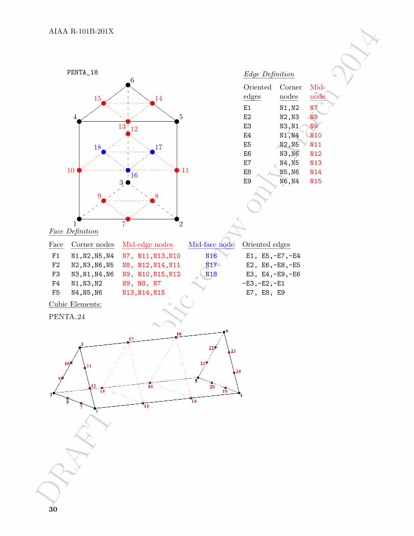
CGNS supports six types of pentahedral elements, PENTA_6, PENTA_15, PENTA_18, PENTA_24,PENTA_38, and PENTA_40. PENTA_6 elements are composed of six nodes located at the six geo-metric corners of the pentahedron. In addition, PENTA_15 and PENTA_18 elements have a node atthe middle of each of the nine edges; PENTA_18 adds a node at the middle of each of the three quadri-lateral faces. The cubic forms of the pentahedral elements, PENTA_24, PENTA_38, and PENTA_40contain two interior nodes along each edge, fourteen interior face nodes in the case of PENTA_38and PENTA_40, and an additonal two interior volume nodes for PENTA_40.


PENTA_6

��ZZZZZZZZ

v1

v2

v3

v4 v5

v6 PENTA_15

��ZZZZZZZZ

v1

v2

v3

v4 v5

v6

v7

v8v9

v10 v11

v12v

13

v14v15

29

DRAFT

-For

publ

icre

view

only

Mar

ch20

14

AIAA R-101B-201X

PENTA_18

��ZZZZZZZZ

v1

v2

v3

v4 v5

v6

v7

v8v9

v10 v11

v12v

13

v14v15

v16

v17v18

Edge Definition

Oriented Corner Mid-edges nodes nodeE1 N1,N2 N7E2 N2,N3 N8E3 N3,N1 N9E4 N1,N4 N10E5 N2,N5 N11E6 N3,N6 N12E7 N4,N5 N13E8 N5,N6 N14E9 N6,N4 N15

Face Definition

Face Corner nodes Mid-edge nodes Mid-face node Oriented edgesF1 N1,N2,N5,N4 N7, N11,N13,N10 N16 E1, E5,-E7,-E4F2 N2,N3,N6,N5 N8, N12,N14,N11 N17 E2, E6,-E8,-E5F3 N3,N1,N4,N6 N9, N10,N15,N12 N18 E3, E4,-E9,-E6F4 N1,N3,N2 N9, N8, N7 -E3,-E2,-E1F5 N4,N5,N6 N13,N14,N15 E7, E8, E9

Cubic Elements:

PENTA 24

30

DRAFT

-For

publ

icre

view

only

Mar

ch20

14

AIAA R-101B-201X

PENTA 38

PENTA 40

Edge Definition

Oriented Corner Mid-edges nodes nodeE1 N1,N2 N7,N8E2 N2,N3 N9,N10E3 N3,N1 N11,N12E4 N1,N4 N13,N14E5 N2,N5 N15,N16E6 N3,N6 N17,N18E7 N4,N5 N19,N20E8 N5,N6 N21,N22E9 N6,N4 N23,N24

31

DRAFT

-For

publ

icre

view

only

Mar

ch20

14

AIAA R-101B-201X

Face Definition

Face Corner nodes Mid-edge nodes Mid-face node Oriented edgesF1 N1,N2,N5,N4 N7,N8,N15,N16,N20,N19,N14,N13 N26,N27,N28,N29 E1, E5,-E7,-E4F2 N2,N3,N6,N5 N9,N10,N17,N18,N22,N21,N16,N15 N30,N31,N32,N33 E2, E6,-E8,-E5F3 N3,N1,N4,N6 N11,N12,N13,N14,N24,N23,N18,N17 N34,N35,N36,N37 E3, E4,-E9,-E6F4 N1,N3,N2 N12,N11,N10,N9,N8,N7 N25 -E3,-E2,-E1F5 N4,N5,N6 N19,N20,N21,N22,N23,N24 N38 E7, E8, E9

Notes

N1,...,N40 Grid point identification number. Integer ≥ 0 or blank, and no two values maybe the same. Grid points N1. . . N3 are in consecutive order about one trilateralface. Grid points N4. . . N6 are in order in the same direction around the oppositetrilateral face.



3.3.3.4 Hexahedral Elements

CGNS supports six types of hexahedral elements, HEXA_8, HEXA_20, HEXA_27, HEXA_32, HEXA_56,and HEXA_64. HEXA_8 elements are composed of eight nodes located at the eight geometric cornersof the hexahedron. In addition, HEXA_20 and HEXA_27 elements have a node at the middle of eachof the twelve edges; HEXA_27 adds a node at the middle of each of the six faces, and one at the cellcenter. The cubic forms of the hexahedral elements, HEXA_32, HEXA_56, and HEXA_64 contain twointerior nodes along each edge, 24 interior face nodes in the case of HEXA_56 and HEXA_64, and anadditonal eight interior volume nodes for HEXA_64.


HEXA_8

��

��

��

v1

v2v3v

4

v5

v6v7v8

HEXA_20

��

��

��

v1

v2v3v

4

v5

v6v7v8

v9

v10

v11

v12

v13

v14v15

v16

v17

v18

v19

v20

32

DRAFT

-For

publ

icre

view

only

Mar

ch20

14

AIAA R-101B-201X

HEXA_27

��

��

��

v1

v2v3v

4

v5

v6v7v8

v9

v10

v11

v12

v13

v14v15

v16

v17

v18

v19

v20

v21

v22

v23

v24

v25

v26

v27

Edge Definition

Oriented Corner Mid-edges nodes nodeE1 N1,N2 N9E2 N2,N3 N10E3 N3,N4 N11E4 N4,N1 N12E5 N1,N5 N13E6 N2,N6 N14E7 N3,N7 N15E8 N4,N8 N16E9 N5,N6 N17E10 N6,N7 N18E11 N7,N8 N19E12 N8,N5 N20

Face Definition

Face Corner nodes Mid-edge nodes Mid-face node Oriented edgesF1 N1,N4,N3,N2 N12,N11,N10,N9 N21 -E4,-E3, -E2, -E1F2 N1,N2,N6,N5 N9, N14,N17,N13 N22 E1, E6, -E9, -E5F3 N2,N3,N7,N6 N10,N15,N18,N14 N23 E2, E7, -E10,-E6F4 N3,N4,N8,N7 N11,N16,N19,N15 N24 E3, E8, -E11,-E7F5 N1,N5,N8,N4 N13,N20,N16,N12 N25 E5,-E12,-E8, E4F6 N5,N6,N7,N8 N17,N18,N19,N20 N26 E9, E10, E11, E12

Cubic Elements:

HEXA 32

33

DRAFT

-For

publ

icre

view

only

Mar

ch20

14

AIAA R-101B-201X

HEXA 56

HEXA 64

34

DRAFT

-For

publ

icre

view

only

Mar

ch20

14

AIAA R-101B-201X

Edge Definition

Oriented Corner Mid-edges nodes nodeE1 N1,N2 N9,N10E2 N2,N3 N11,N12E3 N3,N4 N13,N14E4 N4,N1 N15,N16E5 N1,N5 N17,N18E6 N2,N6 N19,N20E7 N3,N7 N21,N22E8 N4,N8 N23,N24E9 N5,N6 N25,N26E10 N6,N7 N27,N28E11 N7,N8 N29,N30E12 N8,N5 N31,N32

Face Definition

Face Corner nodes Mid-edge nodes Mid-face node Oriented edgesF1 N1,N4,N3,N2 N16,N15,N14,N13,N12,N11,N10,N9 N33,N36,N35,N34 -E4,-E3, -E2, -E1F2 N1,N2,N6,N5 N9,N10,N19,N20,N26,N25,N18,N17 N37,N38,N39,N40 E1, E6, -E9, -E5F3 N2,N3,N7,N6 N11,N12,N21,N22,N28,N27,N20,N19 N41,N42,N43,N44 E2, E7, -E10,-E6F4 N3,N4,N8,N7 N13,N14,N23,N24,N30,N29,N22,N21 N45,N46,N47,N48 E3, E8, -E11,-E7F5 N1,N5,N8,N4 N17,N18,N32,N31,N24,N23,N15,N16 N49,N50,N51,N52 E5,-E12,-E8, E4F6 N5,N6,N7,N8 N25,N26,N27,N28,N29,N30,N31,N32 N53,N54,N55,N56 E9, E10, E11, E12

Notes

N1,...,N64 Grid point identification number. Integer≥ 0 or blank, and no two values may bethe same. Grid points N1. . . N4 are in consecutive order about one quadrilateralface. Grid points N5. . . N8 are in order in the same direction around the oppositequadrilateral face.



3.3.4 Unstructured Grid Example

Consider an unstructured zone in the shape of a cube, with each edge of the zone having threenodes. The resulting unstructured grid has a total of 27 nodes, as illustrated in the exploded figurebelow.

35

DRAFT

-For

publ

icre

view

only

Mar

ch20

14

AIAA R-101B-201X

��

��

��

��

��

s19

s s21

s s ss1

s s3

s s23

ss s14

ss s5

ss25 s s27s s ss7 s s9

��

s19

s20

s21

s10 s11 s12

s1 s2 s3

��

��

��

s25

s26

s27

s16 s17 s18

s7 s8 s9

��

s19

s22

s25

s10

s13

s16

s1

s4

s7��

��

��

s21

s24

s27

s12

s15

s18

s3

s6

s9

This zone contains eight hexahedral cells, numbered 1 to 8, and the cell connectivity is:

Element No. Element Connectivity

1 1, 2, 5, 4, 10, 11, 14, 132 2, 3, 6, 5, 11, 12, 15, 143 4, 5, 8, 7, 13, 14, 17, 164 5, 6, 9, 8, 14, 15, 18, 175 10, 11, 14, 13, 19, 20, 23, 226 11, 12, 15, 14, 20, 21, 24, 237 13, 14, 17, 16, 22, 23, 26, 258 14, 15, 18, 17, 23, 24, 27, 26

In addition to the cells, the boundary faces could also be added to the element definition of thisunstructured zone. There are 24 boundary faces in this zone, corresponding to element numbers 9to 32. Each boundary face is of type QUAD_4. The table below shows the element connectivity ofeach boundary face, as well as the element number and face number of its parent cell.

36

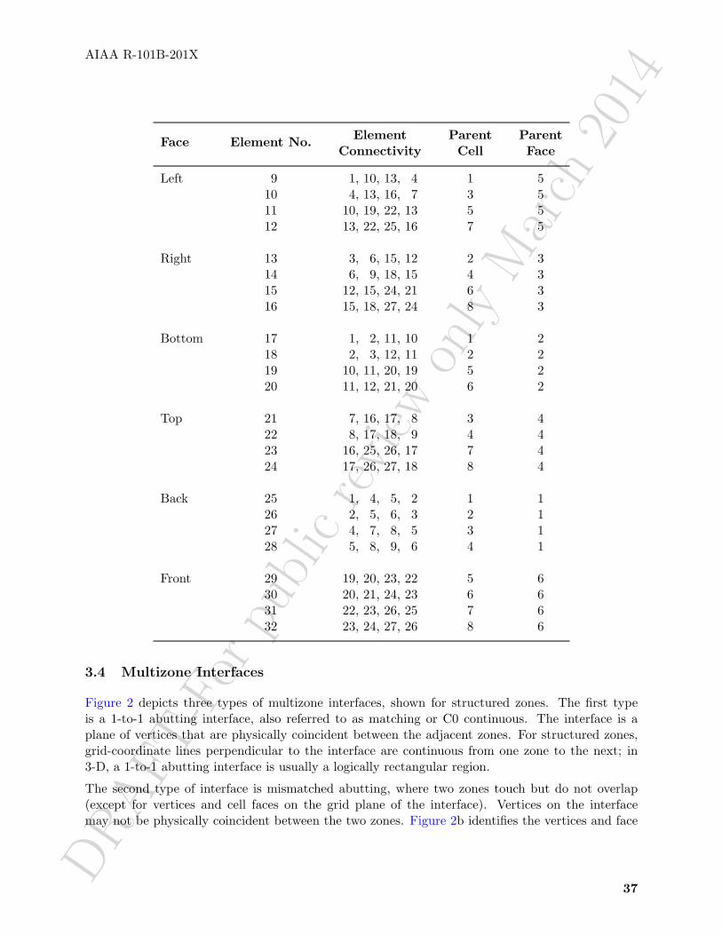
DRAFT

-For

publ

icre

view

only

Mar

ch20

14

AIAA R-101B-201X

Element Parent ParentFace Element No.Connectivity Cell Face

Left 9 1, 10, 13, 4 1 510 4, 13, 16, 7 3 511 10, 19, 22, 13 5 512 13, 22, 25, 16 7 5

Right 13 3, 6, 15, 12 2 314 6, 9, 18, 15 4 315 12, 15, 24, 21 6 316 15, 18, 27, 24 8 3

Bottom 17 1, 2, 11, 10 1 218 2, 3, 12, 11 2 219 10, 11, 20, 19 5 220 11, 12, 21, 20 6 2

Top 21 7, 16, 17, 8 3 422 8, 17, 18, 9 4 423 16, 25, 26, 17 7 424 17, 26, 27, 18 8 4

Back 25 1, 4, 5, 2 1 126 2, 5, 6, 3 2 127 4, 7, 8, 5 3 128 5, 8, 9, 6 4 1

Front 29 19, 20, 23, 22 5 630 20, 21, 24, 23 6 631 22, 23, 26, 25 7 632 23, 24, 27, 26 8 6

3.4 Multizone Interfaces

Figure 2 depicts three types of multizone interfaces, shown for structured zones. The first typeis a 1-to-1 abutting interface, also referred to as matching or C0 continuous. The interface is aplane of vertices that are physically coincident between the adjacent zones. For structured zones,grid-coordinate lines perpendicular to the interface are continuous from one zone to the next; in3-D, a 1-to-1 abutting interface is usually a logically rectangular region.

The second type of interface is mismatched abutting, where two zones touch but do not overlap(except for vertices and cell faces on the grid plane of the interface). Vertices on the interfacemay not be physically coincident between the two zones. Figure 2b identifies the vertices and face

37

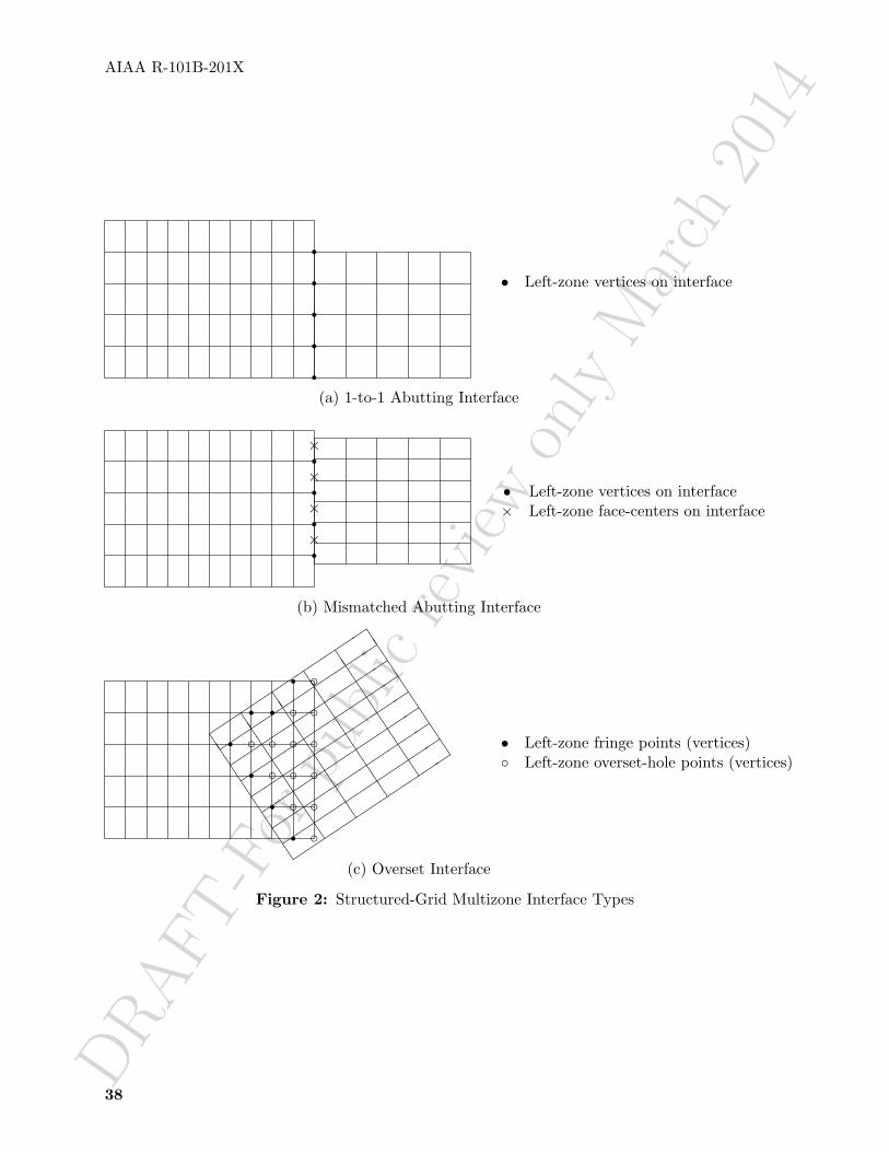
DRAFT

-For

publ

icre

view

only

Mar

ch20

14

AIAA R-101B-201X

rrrrr

• Left-zone vertices on interface

(a) 1-to-1 Abutting Interface

rrrr

××××

• Left-zone vertices on interface× Left-zone face-centers on interface

(b) Mismatched Abutting Interface

rr

rr

r rr

cccccc

cccc

ccc

��

��

��

��

��

��

��

��

��

JJJJJJJJJ

JJJJJJJJJ

JJJJJJJJJ

JJJJJJJJJ

JJJJJJJJJ

JJJJJJJJJ

• Left-zone fringe points (vertices)◦ Left-zone overset-hole points (vertices)

(c) Overset Interface

Figure 2: Structured-Grid Multizone Interface Types

38

DRAFT

-For

publ

icre

view

only

Mar

ch20

14

AIAA R-101B-201X

centers of the left zone that lay on the interface. Even for structured zones in 3-D, the vertices ofa zone that constitute an interface patch may not form a logically rectangular region.

The third type of multizone interface is called overset and occurs when two zones overlap; in 3-D,the overlap is a 3-D region. For overset interfaces, one of the two zones takes precedence over theother; this establishes which solution in the overlap region to retain and which to discard. Theregion in a given zone where the solution is discarded is called an overset hole and the grid pointsoutlining the hole are called fringe points. Figure 2c depicts an overlap region between two zones.The right zone takes precedence over the left zone, and the points identified in the figure are thefringe points and overset-hole points for the left zone. In addition, for the zone taking precedence,any bounding points (i.e., vertices on the bounding faces) of the zone that lay within the overlapregion must also be identified.

Overset interfaces may also include multiple layers of fringe points outlining holes and at zoneboundaries.

For the mismatched abutting and overset interfaces in Figure 2, the left zone plays the role ofreceiver zone and the right plays the role of donor zone.

39

DRAFT

-For

publ

icre

view

only

Mar

ch20

14

DRAFT

-For

publ

icre

view

only

Mar

ch20

14

AIAA R-101B-201X

4 Building-Block Structure Definitions

This section defines and describes low-level structures types that are used in the definition of morecomplex structures within the hierarchy.

4.1 Definition: DataClass_t

DataClass_t is an enumeration type that identifies the class of a given piece of data.

DataClass_t := Enumeration(DataClassNull,DataClassUserDefined,Dimensional,NormalizedByDimensional,NormalizedByUnknownDimensional,NondimensionalParameter,DimensionlessConstant ) ;

These classes divide data into different categories depending on dimensional units or normalizationassociated with the data. Dimensional specifies dimensional data. NormalizedByDimensionalspecifies nondimensional data that is normalized by dimensional reference quantities. In contrast,NormalizedByUnknownDimensional specifies nondimensional data typically found in completelynondimensional databases, where all field and reference data is nondimensional. Nondimension-alParameter specifies nondimensional parameters such as Mach number and lift coefficient. Con-stants such as π are designated by DimensionlessConstant. The distinction between these differentclasses is further discussed in Section 5.

4.2 Definition: Descriptor_t

Descriptor_t is a documentation or annotation structure that contains a character string. Char-acters allowed within the string include newlines, tabs and other special characters; this poten-tially allows for unlimited documentation inclusion within the database. For example, a singleDescriptor_t structure could be used to “swallow” an entire ASCII file. In the hierarchical struc-tures defined in the next sections, each allows for the inclusion of multiple Descriptor_t substruc-tures. Conventions could be made for names of often-used Descriptor_t structure entities, suchas ReadMe or YouReallyWantToReadMeFirst.

Descriptor_t :={Data(char, 1, string_length) ; (r)} ;

where string_length is the length of the character string.

41

DRAFT-Forpublic

review

only


4.3 Definition: DimensionalUnits_t

DimensionalUnits_t describes the system of units used to measure dimensional data. It is com-posed of a set of enumeration types that define the units for mass, length, time, temperature, angle,electric current, substance amount, and luminous intensity.

MassUnits_t := Enumeration( MassUnitsNull, MassUnitsUserDefined,Kilogram, Gram, Slug, PoundMass ) ;

LengthUnits_t := Enumeration( LengthUnitsNull, LengthUnitsUserDefined,Meter, Centimeter, Millimeter, Foot,Inch ) ;

TimeUnits_t := Enumeration( TimeUnitsNull, TimeUnitsUserDefined,Second ) ;

TemperatureUnits_t := Enumeration( TemperatureUnitsNull,TemperatureUnitsUserDefined, Kelvin,Celsius, Rankine, Fahrenheit ) ;

AngleUnits_t := Enumeration( AngleUnitsNull, AngleUnitsUserDefined,Degree, Radian ) ;

ElectricCurrentUnits_t := Enumeration( ElectricCurrentUnitsNull,ElectricCurrentUnitsUserDefined, Ampere,Abampere, Statampere, Edison, auCurrent ) ;

SubstanceAmountUnits_t := Enumeration( SubstanceAmountUnitsNull,SubstanceAmountUnitsUserDefined, Mole,Entities, StandardCubicFoot,StandardCubicMeter ) ;

LuminousIntensityUnits_t := Enumeration( LuminousIntensityUnitsNull,LuminousIntensityUnitsUserDefined,Candela, Candle, Carcel, Hefner, Violle ) ;

DimensionalUnits_t :={MassUnits_t MassUnits ; (r)LengthUnits_t LengthUnits ; (r)TimeUnits_t TimeUnits ; (r)TemperatureUnits_t TemperatureUnits ; (r)AngleUnits_t AngleUnits ; (r)AdditionalUnits_t := (o){

42

DRAFT-Forpublic

review

only


ElectricCurrentUnits_t ElectricCurrentUnits ; (r)SubstanceAmountUnits_t SubstanceAmountUnits ; (r)LuminousIntensityUnits_t LuminousIntensityUnits ; (r)}

} ;

The International System (SI) uses the following units.

Physical Quantity Unit

Mass KilogramLength MeterTime SecondTemperature KelvinAngle RadianElectric Current AmpereSubstance Amount MoleLuminous Intensity Candela

For an entity of type DimensionalUnits_t, if all the elements of that entity have the value Null(i.e., MassUnits = MassUnitsNull, etc.), this is equivalent to stating that the data described bythe entity is nondimensional.

4.4 Definition: DimensionalExponents_t

DimensionalExponents_t describes the dimensionality of data by defining the exponents associatedwith each of the fundamental units.

DimensionalExponents_t :={real MassExponent ; (r)real LengthExponent ; (r)real TimeExponent ; (r)real TemperatureExponent ; (r)real AngleExponent ; (r)AdditionalExponents_t := (o){real ElectricCurrentExponent ; (r)real SubstanceAmountExponent ; (r)real LuminousIntensityExponent ; (r)}

} ;

For example, an instance of DimensionalExponents_t that describes velocity is,

43

DRAFT

-For

publ

icre

view

only

Mar

ch20

14

AIAA R-101B-201X

DimensionalExponents_t ={{MassExponent = 0 ;LengthExponent = +1 ;TimeExponent = -1 ;TemperatureExponent = 0 ;AngleExponent = 0 ;}} ;

4.5 Definition: GridLocation_t

GridLocation_t identifies locations with respect to the grid; it is an enumeration type.

GridLocation_t := Enumeration(GridLocationNull,GridLocationUserDefined,Vertex,CellCenter,FaceCenter,IFaceCenter,JFaceCenter,KFaceCenter,EdgeCenter ) ;

Vertex is coincident with the grid vertices. CellCenter is the center of a cell; this is also appropriatefor entities associated with cells but not necessarily with a given location in a cell. For structuredzones, IFaceCenter is the center of a face in 3-D whose computational normal points in the idirection. JFaceCenter and KFaceCenter are similarly defined, again only for structured zones.FaceCenter is the center of a generic face that can point in any coordinate direction. These arealso appropriate for entities associated with a face, but not located at a specific place on the face.EdgeCenter is the center of an edge. See Section 3.2 for descriptions of cells, faces and edges.

All of the entities of type GridLocation_t defined in this document use a default value of Vertex.

4.6 Definition: IndexArray_t

IndexArray_t specifies an array of indices. An argument is included that allows for specifying thedata type of each index; typically the data type will be integer (int). IndexArray_t defines anarray of indices of size ArraySize, where the dimension of each index is IndexDimension.

IndexArray_t< int IndexDimension, int ArraySize, DataType > :={Data( DataType, 2, [IndexDimension,ArraySize] ) ; (r)} ;

44

DRAFT

-For

publ

icre

view

only

Mar

ch20

14

AIAA R-101B-201X

4.7 Definition: IndexRange_t

IndexRange_t specifies the beginning and ending indices of a subrange. The subrange may describea portion of a grid line, grid plane, or grid volume.

IndexRange_t< int IndexDimension > :={int[IndexDimension] Begin ; (r)int[IndexDimension] End ; (r)} ;

where Begin and End are the indices of the opposing corners of the subrange.

4.8 Definition: Rind_t

Rind_t describes the number of rind planes (for structured grids) or rind points and elements (forunstructured grids) associated with a data array containing grid coordinates, flow-solution data orany other grid-related discrete data.

Rind_t< int IndexDimension > :={int[2*IndexDimension] RindPlanes ; (r)} ;

For structured grids, RindPlanes contains the number of rind planes attached to the minimum andmaximum faces of a zone. The face corresponding to each index n of RindPlanes in 3-D is:

n = 1 → i-min n = 2 → i-maxn = 3 → j-min n = 4 → j-maxn = 5 → k-min n = 6 → k-max

For a 3-D grid whose “core” size is II×JJ×KK, a value of RindPlanes = [a,b,c,d,e,f] indicatesthat the range of indices for the grid with rind is:

i: (1 - a, II + b)j: (1 - c, JJ + d)k: (1 - e, KK + f)

For unstructured grids, RindPlanes does not actually contain planes, but rather contains thenumber of rind points or elements. The points are defined by the grid coordinates rind node, andthe elements by the element set rind node. Note that to maintain consistency with the structuredusage of Rind_t, RindPlanes is still dimensioned 2*IndexDimension for unstructured grids (and,for unstructured grids, IndexDimension = 1). The first RindPlanes value is the number of rindnodes/elements stored before the core data, and the second is the number stored after. ThusRindPlanes[2] = [1 2] would mean there is one rind value before the core data, and two afterthe core data. However, it is preferable to write all the rind points or elements at the end of thearray; in other words, for unstructured grids RindPlanes[2] should be set to [0 nrind], wherenrind is the number of rind points or elements.

45

DRAFT

-For

publ

icre

view

only

Mar

ch20

14

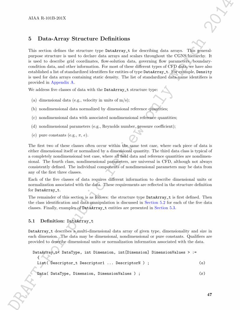
DRAFT-Forpublic

review

only


5 Data-Array Structure Definitions

This section defines the structure type DataArray_t for describing data arrays. This general-purpose structure is used to declare data arrays and scalars throughout the CGNS hierarchy. Itis used to describe grid coordinates, flow-solution data, governing flow parameters, boundary-condition data, and other information. For most of these different types of CFD data, we have alsoestablished a list of standardized identifiers for entities of type DataArray_t. For example, Densityis used for data arrays containing static density. The list of standardized data-name identifiers isprovided in Appendix A.

We address five classes of data with the DataArray_t structure type:

(a) dimensional data (e.g., velocity in units of m/s);

(b) nondimensional data normalized by dimensional reference quantities;

(c) nondimensional data with associated nondimensional reference quantities;

(d) nondimensional parameters (e.g., Reynolds number, pressure coefficient);

(e) pure constants (e.g., π, e).

The first two of these classes often occur within the same test case, where each piece of data iseither dimensional itself or normalized by a dimensional quantity. The third data class is typical ofa completely nondimensional test case, where all field data and reference quantities are nondimen-sional. The fourth class, nondimensional parameters, are universal in CFD, although not alwaysconsistently defined. The individual components of nondimensional parameters may be data fromany of the first three classes.

Each of the five classes of data requires different information to describe dimensional units ornormalization associated with the data. These requirements are reflected in the structure definitionfor DataArray_t.

The remainder of this section is as follows: the structure type DataArray_t is first defined. Thenthe class identification and data manipulation is discussed in Section 5.2 for each of the five dataclasses. Finally, examples of DataArray_t entities are presented in Section 5.3.

5.1 Definition: DataArray_t

DataArray_t describes a multi-dimensional data array of given type, dimensionality and size ineach dimension. The data may be dimensional, nondimensional or pure constants. Qualifiers areprovided to describe dimensional units or normalization information associated with the data.

DataArray_t< DataType, int Dimension, int[Dimension] DimensionValues > :={List( Descriptor_t Descriptor1 ... DescriptorN ) ; (o)

Data( DataType, Dimension, DimensionValues ) ; (r)

47

DRAFT-Forpublic

review

only


DataClass_t DataClass ; (o)

DimensionalUnits_t DimensionalUnits ; (o)

DimensionalExponents_t DimensionalExponents ; (o)

DataConversion_t DataConversion ; (o)} ;

Notes

1. Default names for the Descriptor_t list are as shown; users may choose other legitimatenames. Legitimate names must be unique within a given instance of DataArray_t andshall not include the names DataClass, DimensionalUnits, DimensionalExponents, orDataConversion.

2. Data() is the only required field for DataArray_t.

DataArray_t requires three structure parameters: Dimension is the dimensionality of the dataarray; DimensionValues is an array of length Dimension that contains the size of the data arraysin each dimension; and DataType is the data type of the data stored. DataType will usually bereal, but other data types are permissible.

The optional entities DataClass, DimensionalUnits, DimensionalExponents and DataConver-sion provide information on dimensional units and normalization associated with the data. Thefunction of these qualifiers is provided in the next section.

This structure type is formulated to describe an array of scalars. Therefore, for vector quantities(e.g., the position vector or the velocity vector), separate structure entities are required for eachcomponent of the vector. For example, the Cartesian coordinates of a 3-D grid are described bythree separate DataArray_t entities: one for x, one for y and one for z (see Example 7-A).

5.1.1 Definition: DataConversion_t

DataConversion_t contains conversion factors for recovering raw dimensional data from givennondimensional data. These conversion factors are typically associated with nondimensional datathat is normalized by dimensional reference quantities.

DataConversion_t :={real ConversionScale ; (r)

real ConversionOffset ; (r)} ;

Given a nondimensional piece of data, Data(nondimensional), the conversion to“raw”dimensionalform is:

48

DRAFT

-For

publ

icre

view

only

Mar

ch20

14

AIAA R-101B-201X

Data(raw) = Data(nondimensional)*ConversionScale + ConversionOffset

These conversion factors are further described in Section 5.2.2.

5.2 Data Manipulation

The optional entities of DataArray_t provide information for manipulating the data, includingchanging units or normalization. This section describes the rules under which these optional entitiesoperate and the specific manipulations that can be performed on the data.

Within a given instance of DataArray_t, the class of data and all information required for manip-ulations may be completely and precisely specified by the entities DataClass, DimensionalUnits,DimensionalExponents and DataConversion. DataClass identifies the class of data and governsthe manipulations that can be performed. Each of the five data classes is treated separately in thesubsequent sections.

The entities DataClass and DimensionalUnits serve special functions in the CGNS hierarchy.If DataClass is absent from a given instance of DataArray_t, then its value is determined from“global” data. This global data may be set at any level of the CGNS hierarchy with the data set atthe lowest level taking precedence. DimensionalUnits may be similarly set by global data. Therules for determining the appropriate set of global data to apply is further detailed in Section 6.4.

This alternate functionality provides a measure of economy in describing dimensional units or nor-malization within the hierarchy. Examples that make use of global data are presented in Section 7.2and Section 7.8 for grid and flow solution data. The complete two-zone case of Appendix B alsodepicts this alternate functionality.

5.2.1 Dimensional Data

If DataClass = Dimensional, the data is dimensional. The optional qualifiers DimensionalUnitsand DimensionalExponents describe dimensional units associated with the data. These qualifiersare provided to specify the system of dimensional units and the dimensional exponents, respectively.For example, if the data is the x-component of velocity, then DimensionalUnits will state that thepertinent dimensional units are, say, Meter and Second; DimensionalExponents will specify thatthe pertinent dimensional exponents are LengthExponent = 1 and TimeExponent = -1. Combiningthe information gives the units m/s. Examples showing the use of these two qualifiers are providedin Section 5.3.

If DimensionalUnits is absent, then the appropriate set of dimensional units is obtained from“global” data. The rules for determining this appropriate set of global dimensional units are pre-sented in Section 6.4.

If DimensionalExponents is absent, then the appropriate dimensional exponents can be determinedby convention if the specific instance of DataArray_t corresponds to one of the standardized data-name identifiers listed in Appendix A. Otherwise, the exponents are unspecified. We stronglyrecommend inclusion of the DimensionalExponents qualifier whenever the data is dimensionaland the instance of DataArray_t is not among the list of standardized identifiers.

49

DRAFT

-For

publ

icre

view

only

Mar

ch20

14

AIAA R-101B-201X

5.2.2 Nondimensional Data Normalized by Dimensional Quantities

If DataClass = NormalizedByDimensional, the data is nondimensional and is normalized by di-mensional reference quantities. All optional entities in DataArray_t are used. DataConversioncontains factors to convert the nondimensional data to “raw” dimensional data; these factors areConversionScale and ConversionOffset. The conversion process is as follows:

Data(raw) = Data(nondimensional)*ConversionScale + ConversionOffset

where Data(nondimensional) is the original nondimensional data, and Data(raw) is the convertedraw data. This converted raw data is dimensional, and the optional qualifiers DimensionalUnitsand DimensionalExponents describe the appropriate dimensional units and exponents. Note thatDimensionalUnits and DimensionalExponents also describe the units for ConversionScale andConversionOffset.

If DataConversion is absent, the equivalent defaults are ConversionScale = 1 and Conver-sionOffset = 0. If either DimensionalUnits or DimensionalExponents is absent, follow therules described in the previous section.

Note that functionally there is little difference between these first two data classes (DataClass =Dimensional and NormalizedByDimensional). In the first case the data is dimensional, and inthe second, the converted raw data is dimensional. Also, the equivalent defaults for DataConver-sion produce no changes in the data; hence, it is almost the same as stating the original data isdimensional.

5.2.3 Nondimensional Data Normalized by Unknown Dimensional Quantities

If DataClass = NormalizedByUnknownDimensional, the data is nondimensional and is normalizedby some unspecified dimensional quantities. This type of data is typical of a completely nondimen-sional test case, where all field data and all reference quantities are nondimensional.

Only the DimensionalExponents qualifier is used in this case, although it is expected that thisqualifier will be seldom utilized in practice. For entities of DataArray_t that are not among thelist of standardized data-name identifiers, the qualifier could provide useful information by definingthe exponents of the dimensional form of the nondimensional data.

Rather than providing qualifiers to describe the normalization of the data, we instead dictate thatall data of type NormalizedByUnknownDimensional in a given database be nondimensionalizedconsistently. This is done by picking one set of mass, length, time and temperature scales andnormalizing all appropriate data by these scales. We describe this process in detail in the following.Appendix B also shows a completely nondimensional database where consistent normalization isused throughout.

The practice of nondimensionalization within flow solvers and other application codes is quitepopular. The problem with this practice is that to manipulate the data from a given code, one mustoften know the particulars of the nondimensionalization used. This largely results from what wecall inconsistent normalization—more than the minimum required scales are used to normalize data

50

DRAFT

-For

publ

icre

view

only

Mar

ch20

14

AIAA R-101B-201X

within the code. For example, in the OVERFLOW flow solver, the following nondimensionalizationis used:

x = x/L, u = u/c∞, ρ = ρ/ρ∞,y = y/L, v = v/c∞, p = p/(ρ∞c2

∞),z = z/L, w = w/c∞, µ = µ/µ∞,

where (x, y, z) are the Cartesian coordinates, (u, v, w) are the Cartesian components of velocity, ρis static density, p is static pressure, c is the static speed of sound, and µ is the molecular viscosity.In this example, tilde quantities ( ) are nondimensional and all others are dimensional. Four dimen-sional scales are used for normalization: L (a unit length), ρ∞, c∞ and µ∞. However, only threefundamental dimensional units are represented: mass, length and time. The extra normalizingscale leads to inconsistent normalization. The primary consequence of this is additional nondi-mensional parameters, such as Reynolds number, appearing in the nondimensionalized governingequations where none are found in the original dimensional equations. Many definitions, includingskin friction coefficient, also have extra terms appearing in the nondimensionalized form. This addsunnecessary complication to any data or equation manipulation associated with the flow solver.

Consistent normalization avoids many of these problems. Here the number of scales used fornormalization is the same as the number of fundamental dimensional units represented by thedata. Using consistent normalization, the resulting nondimensionalized form of equations anddefinitions is identical to their original dimensional formulations. One piece of evidence to supportthis assertion is that it is not possible to form any nondimensional parameters from the set ofdimensional scales used for normalization.

An important fallout of consistent normalization is that the actual scales used for normalizationbecome immaterial for all data manipulation processes. To illustrate this consider the followingnondimensionalization procedure: let M (mass), L (length) and T (time) be arbitrary dimensionalscales by which all data is normalized (neglect temperature data for the present). The nondimen-sional data follows:

x′ = x/L, u′ = u/(L/T ), ρ′ = ρ/(M/L3),y′ = y/L, v′ = v/(L/T ), p′ = p/(M/(LT 2)),z′ = z/L, w′ = w/(L/T ), µ′ = µ/(M/(LT )),

where primed quantities are nondimensional and all others are dimensional.

Consider an existing database where all field data and all reference data is nondimensional andnormalized as shown. Assume the database has a single reference state given by,

x′ref = xref/L, u′ref = uref/(L/T ), ρ′ref = ρref/(M/L3),y′ref = yref/L, v′ref = vref/(L/T ), p′ref = pref/(M/(LT 2))z′ref = zref/L, w′ref = wref/(L/T ), µ′ref = µref/(M/(LT )).

If a user wanted to change the nondimensionalization of grid-point pressures, the procedure isstraightforward. Let the desired new normalization be given by p′′ijk = pijk/(ρrefc

2ref), where all

terms on the right-hand-side are dimensional, and as such they are unknown to the database user.However, the desired manipulation is possible using only nondimensional data provided in the

51

DRAFT

-For

publ

icre

view

only

Mar

ch20

14

AIAA R-101B-201X

database,p′′ijk ≡ pijk/(ρrefc

2ref)

=pijk

M/(LT 2)M/L3

ρref

[L/T

cref

]2

= p′ijk/(ρ′ref(c

′ref)

2)

Thus, the desired renormalization is possible using the database’s nondimensional data as if it wereactually dimensional. There is, in fact, a high degree of equivalence between dimensional data andconsistently normalized nondimensional data. The procedure shown in this example should extendto any desired renormalization, provided the needed reference-state quantities are included in thedatabase.

This example points out two stipulations that we now dictate for data in the class Normalized-ByUnknownDimensional,

(a) All nondimensional data within a given database that has DataClass = NormalizedByUn-knownDimensional shall be consistently normalized.

(b) Any nondimensional reference state appearing in a database should be sufficiently populatedwith reference quantities to allow for renormalization procedures.

The second of these stipulations is somewhat ambiguous, but good practice would suggest that aflow solver, for example, should output to the database enough static and/or stagnation referencequantities to sufficiently define the state.

Appendix B shows an example of a well-populated reference state.

With these two stipulations, we contend the following:

• The dimensional scales used to nondimensionalize all data are immaterial, and there is noneed to identify these quantities in a CGNS database.

• The dimensional scales need not be reference-state quantities provided in the database. Forexample, a given database could contain freestream reference state conditions, but all thedata is normalized by sonic conditions (which are not provided in the database).

• All renormalization procedures can be carried out treating the data as if it were dimensionalwith a consistent set of units.

• Any application code that internally uses consistent normalization can use the data providedin a CGNS database without modification or transformation to the code’s internal normal-ization.

Before ending this section, we note that the OVERFLOW flow solver mentioned above (or anyother application code that internally uses inconsistent normalization) could easily read and writedata to a nondimensional CGNS database that conforms to the above stipulations. On output, thecode could renormalize data so it is consistently normalized. Probably, the easiest method would

52

DRAFT

-For

publ

icre

view

only

Mar

ch20

14

AIAA R-101B-201X

be to remove the molecular viscosity scale (µ∞), and only use L, ρ∞ and c∞ for all normalizations(recall these are dimensional scales). The only change from the above example would be thenondimensionalization of viscosity, which would become, ˜µ = µ/(ρ∞c∞L). The code could thenoutput all field data as,

xijk = xijk/L, uijk = uijk/c∞, ρijk = ρijk/ρ∞,yijk = yijk/L, vijk = vijk/c∞, pijk = pijk/(ρ∞c2

∞),zijk = zijk/L, wijk = wijk/c∞, ˜µijk = µijk/(ρ∞c∞L),

and output the freestream reference quantities,

u∞ = u∞/c∞, ρ∞ = ρ∞/ρ∞ = 1,v∞ = v∞/c∞, p∞ = p∞/(ρ∞c2

∞) = 1/γ,w∞ = w∞/c∞, ˜µ∞ = µ∞/(ρ∞c∞L) ∼ O(1/Re),c∞ = c∞/c∞ = 1, L = L/L = 1,

where γ is the specific heat ratio (assumes a perfect gas) and Re is the Reynolds number.

On input, the flow solver should be able to recover its internal normalizations from the data in anondimensional CGNS database by treating the data as if it were dimensional.

5.2.4 Nondimensional Parameters

If DataClass = NondimensionalParameter, the data is a nondimensional parameter (or arrayof nondimensional parameters). Examples include Mach number, Reynolds number and pressurecoefficient. These parameters are prevalent in CFD, although their definitions tend to vary be-tween different application codes. A list of standardized data-name identifiers for nondimensionalparameters is provided in Appendix A.4.

We distinguish nondimensional parameters from other data classes by the fact that they are alwaysdimensionless. In a completely nondimensional database, they are distinct in that their normaliza-tion is not necessarily consistent with other data.

Typically, the DimensionalUnits, DimensionalExponents and DataConversion qualifiers are notused for nondimensional parameters; although, there are a few situations where they may be used(these are discussed below). Rather than rely on optional qualifiers to describe the normalization,we establish the convention that any nondimensional parameters should be accompanied by theirdefining scales; this is further discussed in Appendix A.4. An example is Reynolds number definedas Re = V LR/ν, where V , LR and ν are velocity, length, and viscosity scales, respectively. Notethat these defining scales may be dimensional or nondimensional data. We establish the data-nameidentifiers Reynolds, Reynolds_Velocity, Reynolds_Length and Reynolds_ViscosityKinematicfor the Reynolds number and its defining scales. Anywhere an instance of DataArray_t is foundwith the identifier Reynolds, there should also be entities for the defining scales. An example ofthis use for Reynolds number is given in Section 5.3.

In certain situations, it may be more convenient to use the optional qualifiers of DataArray_t todescribe the normalization used in nondimensional parameters. These situations must satisfy tworequirements: First, the defining scales are dimensional; and second, the nondimensional parameter

53

DRAFT-Forpublic

review

only


is a normalization of a single “raw” data quantity and it is clear what this raw data is. Examplesthat satisfy this second constraint are pressure coefficient, where the raw data is static pressure, andlift coefficient, where the raw data is the lift force. Conversely, Reynolds number is a parameterthat violates the second requirement—there are three pieces of raw data rather than one thatmake up Re. For nondimensional parameters that satisfy these two requirements, the qualifiersDimensionalUnits, DimensionalExponents and DataConversion may be used as in Section 5.2.2to recover the raw dimensional data.

5.2.5 Dimensionless Constants

If DataClass = DimensionlessConstant, the data is a constant (or array of constants) with no as-sociated dimensional units. The DimensionalUnits, DimensionalExponents and DataConversionqualifiers are not used.

5.3 Data-Array Examples

This section presents five examples of data-array entities and illustrates the use of optional infor-mation for describing dimensional and nondimensional data.

Example 5-A: One-Dimensional Data Array, Constants

A one-dimensional array of integers; the array is the integers from 1 to 10. The data is pureconstants.

! DataType = int! Dimension = 1! DimensionValues = 10DataArray_t<int, 1, 10> Data1 ={{Data(int, 1, 10) = [1, 2, 3, 4, 5, 6, 7, 8, 9, 10] ;

DataClass_t DataClass = DimensionlessConstant ;}} ;

The structure parameters for DataArray_t state the data is an one-dimensional integer array oflength ten. The value of DataClass indicates the data is unitless constants.

Example 5-B: Two-Dimensional Data Array, Pressures

A two-dimensional array of pressures with size 11 × 9 given by the array P(i,j). The data isdimensional with units of N/m2 (i.e., kg/(m-s2)). Note that Pressure is the data-name identifierfor static pressure.

! DataType = real! Dimension = 2! DimensionValues = [11,9]

54

DRAFT-Forpublic

review

only


DataArray_t<real, 2, [11,9]> Pressure ={{Data(real, 2, [11,9]) = ((P(i,j), i=1,11), j=1,9) ;

DataClass_t DataClass = Dimensional ;

DimensionalUnits_t DimensionalUnits ={{MassUnits = Kilogram ;LengthUnits = Meter ;TimeUnits = Second ;TemperatureUnits = TemperatureUnitsNull ;AngleUnits = AngleUnitsNull ;}} ;

DimensionalExponents_t DimensionalExponents ={{MassExponent = +1 ;LengthExponent = -1 ;TimeExponent = -2 ;TemperatureExponent = 0 ;AngleExponent = 0 ;}} ;

}} ;

From the data-name identifier conventions presented in Appendix A, Pressure has a floating-pointdata type; hence, the appropriate structure parameter for DataArray_t is real.

The value of DataClass indicates that the data is dimensional, and both the dimensional unitsand dimensional exponents are provided. DimensionalUnits specifies that the units are kilograms,meters, and seconds, and DimensionalExponents specifies the appropriate exponents for pressure.Combining the information gives pressure as kg/(m-s2). DimensionalExponents could have beendefaulted, since the dimensional exponents are given in Appendix A for the data-name identifierPressure.

Note that FORTRAN multidimensional array indexing is used to store the data; this is reflected inthe FORTRAN-like implied do-loops for P(i,j).

Example 5-C: Three-Dimensional Data Array, Nondimensional Static Enthalpy

A 3-D array of size 33× 9× 17 containing nondimensional static enthalpy. The data is normalizedby freestream velocity as follows:

hi,j,k =hi,j,kq2

ref

,

where hi,j,k is nondimensional static enthalpy. The freestream velocity is dimensional with a valueof 10 m/s.

55

DRAFT-Forpublic

review

only


! DataType = real! Dimension = 3! DimensionValues = [33,9,17]DataArray_t<real, 3, [33,9,17]> Enthalpy ={{Data(real, 3, [33,9,17]) = (((H(i,j,k), i=1,33), j=1,9), k=1,17) ;

DataClass_t DataClass = NormalizedByDimensional ;

DataConversion_t DataConversion ={{real ConversionScale = 100 ;real ConversionOffset = 0 ;}} ;

DimensionalUnits_t DimensionalUnits ={{MassUnits = MassUnitsNull ;LengthUnits = Meter ;TimeUnits = Second ;TemperatureUnits = TemperatureUnitsNull ;AngleUnits = AngleUnitsNull ;}} ;

DimensionalExponents_t DimensionalExponents ={{MassExponent = 0 ;LengthExponent = +2 ;TimeExponent = -2 ;TemperatureExponent = 0 ;AngleExponent = 0 ;}} ;

}} ;

From Appendix A, the identifier for static enthalpy is Enthalpy and its data type is real.

The value of DataClass indicates that the data is nondimensional and normalized by a dimensionalreference quantity. DataConversion provides the conversion factors for recovering the raw staticenthalpy, which has units of m2/s2 as indicated by DimensionalUnits and DimensionalExponents.Note that DimensionalExponents could have been defaulted using the conventions for the data-name identifier Enthalpy.

Example 5-D: Three-Dimensional Data Array, Nondimensional Database

The previous example for nondimensional enthalpy is repeated for a completely nondimensionaldatabase.

56

DRAFT

-For

publ

icre

view

only

Mar

ch20

14

AIAA R-101B-201X

! DataType = real! Dimension = 3! DimensionValues = [33,9,17]DataArray_t<real, 3, [33,9,17]> Enthalpy ={{Data(real, 3, [33,9,17]) = (((H(i,j,k), i=1,33), j=1,9), k=1,17) ;

DataClass_t DataClass = NormalizedByUnknownDimensional ;}} ;

The value of DataClass indicates the appropriate class.

Example 5-E: Data Arrays for Reynolds Number

Reynolds number of 1.554×106 based on a velocity scale of 10 m/s, a length scale of 2.3 m anda kinematic viscosity scale of 1.48×10−5 m2/s. Assume the database has globally set the dimen-sional units to kilograms, meters, and seconds, and the global default data class to dimensional(DataClass = Dimensional).

! DataType = real! Dimension = 1! DimensionValues = 1DataArray_t<real, 1, 1> Reynolds ={{Data(real, 1, 1) = 1.554e+06 ;

DataClass_t DataClass = NondimensionalParameter ;}} ;

DataArray_t<real, 1, 1> Reynolds_Velocity ={{Data(real, 1, 1) = 10. ;}} ;

DataArray_t<real, 1, 1> Reynolds_Length ={{Data(real, 1, 1) = 2.3 ;}} ;

DataArray_t<real, 1, 1> Reynolds_ViscosityKinematic ={{Data(real, 1, 1) = 1.48e-05 ;}} ;

Reynolds contains the value of the Reynolds number, and the value of its DataClass qualifierdesignates it as a nondimensional parameter. By conventions described in Appendix A.4, the

57

DRAFT

-For

publ

icre

view

only

Mar

ch20

14

AIAA R-101B-201X

defining scales are contained in the associated entities Reynolds_Velocity, Reynolds_Length,and Reynolds_ViscosityKinematic. Since each of these entities contain no qualifiers, globalinformation is used to decipher that they are all dimensional with mass, length, and time units ofkilograms, meters, and seconds. The structure parameters for each DataArray_t entity state thatthey contain a real scalar.

If a user wanted to convey the dimensional units of the defining scales using optional qualifiersof DataArray_t, then the last three entities in this example would have a form similar to that inExample 5-B.

58

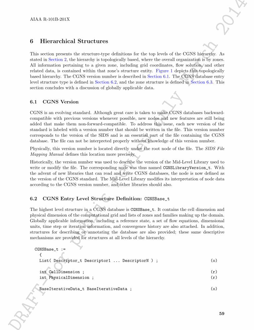
DRAFT-Forpublic

review

only


6 Hierarchical Structures

This section presents the structure-type definitions for the top levels of the CGNS hierarchy. Asstated in Section 2, the hierarchy is topologically based, where the overall organization is by zones.All information pertaining to a given zone, including grid coordinates, flow solution, and otherrelated data, is contained within that zone’s structure entity. Figure 1 depicts this topologicallybased hierarchy. The CGNS version number is described in Section 6.1. The CGNS database entrylevel structure type is defined in Section 6.2, and the zone structure is defined in Section 6.3. Thissection concludes with a discussion of globally applicable data.

6.1 CGNS Version

CGNS is an evolving standard. Although great care is taken to make CGNS databases backward-compatible with previous versions whenever possible, new nodes and new features are still beingadded that make them non-forward-compatible. To address this issue, each new version of thestandard is labeled with a version number that should be written in the file. This version numbercorresponds to the version of the SIDS and is an essential part of the file containing the CGNSdatabase. The file can not be interpreted properly without knowledge of this version number.

Physically, this version number is located directly under the root node of the file. The SIDS FileMapping Manual defines this location more precisely.

Historically, the version number was used to describe the version of the Mid-Level Library used towrite or modify the file. The corresponding node was thus named CGNSLibraryVersion_t. Withthe advent of new libraries that can read and write CGNS databases, the node is now defined asthe version of the CGNS standard. The Mid-Level Library modifies its interpretation of node dataaccording to the CGNS version number, and other libraries should also.

6.2 CGNS Entry Level Structure Definition: CGNSBase_t

The highest level structure in a CGNS database is CGNSBase_t. It contains the cell dimension andphysical dimension of the computational grid and lists of zones and families making up the domain.Globally applicable information, including a reference state, a set of flow equations, dimensionalunits, time step or iteration information, and convergence history are also attached. In addition,structures for describing or annotating the database are also provided; these same descriptivemechanisms are provided for structures at all levels of the hierarchy.

CGNSBase_t :={List( Descriptor_t Descriptor1 ... DescriptorN ) ; (o)

int CellDimension ; (r)int PhysicalDimension ; (r)

BaseIterativeData_t BaseIterativeData ; (o)

59

DRAFT

-For

publ

icre

view

only

Mar

ch20

14

AIAA R-101B-201X

List( Zone_t<CellDimension, PhysicalDimension> Zone1 ... ZoneN ) ; (o)

ReferenceState_t ReferenceState ; (o)

Axisymmetry_t Axisymmetry ; (o)

RotatingCoordinates_t RotatingCoordinates ; (o)

Gravity_t Gravity ; (o)

SimulationType_t SimulationType ; (o)



FlowEquationSet_t<CellDimension> FlowEquationSet ; (o)

ConvergenceHistory_t GlobalConvergenceHistory ; (o)

List( IntegralData_t IntegralData1... IntegralDataN ) ; (o)

List( Family_t Family1... FamilyN ) ; (o)

List( UserDefinedData_t UserDefinedData1 ... UserDefinedDataN ) ; (o)} ;

Notes

1. Default names for the Descriptor_t, Zone_t, IntegralData_t, Family_t, and UserDe-finedData_t lists are as shown; users may choose other legitimate names. Legitimate namesmust be unique at this level and shall not include the names Axisymmetry, BaseItera-tiveData, DataClass, DimensionalUnits, FlowEquationSet, GlobalConvergenceHistory,Gravity, ReferenceState, RotatingCoordinates, or SimulationType.

2. The number of entities of type Zone_t defines the number of zones in the domain.3. CellDimension and PhysicalDimension are the only required fields. The Descriptor_t,

Zone_t and IntegralData_t lists may be empty, and all other optional fields absent.

Note that we make the distinction between the following:

IndexDimension Number of different indices required to reference a node (e.g., 1 = i,2 = i, j, 3 = i, j, k)

CellDimension Dimensionality of the cell in the mesh (e.g., 3 for a volume cell, 2 for aface cell)

60

DRAFT

-For

publ

icre

view

only

Mar

ch20

14

AIAA R-101B-201X

PhysicalDimension Number of coordinates required to define a node position (e.g., 1 for1-D, 2 for 2-D, 3 for 3-D)

These three dimensions may differ depending on the mesh. For example, an unstructured triangularsurface mesh representing the wet surface of an aircraft will have:

• IndexDimension = 1 (always for unstructured)

• CellDimension = 2 (face elements)

• PhysicalDimension = 3 (needs x, y, z coordinates since it is a 3D surface)

For a structured zone, the quantities IndexDimension and CellDimension are always equal. Foran unstructured zone, IndexDimension always equals 1. Therefore, storing CellDimension at theCGNSBase_t level will automatically define the IndexDimension value for each zone.

On the other hand we assume that all zones of the base have the same CellDimension, e.g., ifCellDimension is 3, all zones must be composed of 3D cells within the CGNSBase_t.

We need IndexDimension for both structured and unstructured zones in order to use original datastructures such as GridCoordinates_t, FlowSolution_t, DiscreteData_t, etc. CellDimensionis necessary to express the interpolants in ZoneConnectivity with an unstructured zone (mis-match or overset connectivity). When the cells are bidimensional, two interpolants per node arerequired, whereas when the cells are tridimensional, three interpolants per node must be provided.PhysicalDimension becomes useful when expressing quantities such as the InwardNormalList inthe BC_t data structure. It’s possible to have a mesh where IndexDimension = 2 but the normalvectors still require x, y, z components in order to be properly defined. Consider, for example, astructured surface mesh in the 3D space.

Information about the number of time steps or iterations being recorded, and the time and/oriteration values at each step, may be contained in the BaseIterativeData structure.

Data specific to each zone in a multizone case is contained in the list of Zone_t structure entities.

Reference data applicable to the entire CGNS database is contained in the ReferenceState struc-ture; quantities such as Reynolds number and freestream Mach number are contained here (forexternal flow problems).

Axisymmetry may be used to specify the axis of rotation and the circumferential extent for anaxisymmetric database.

If a rotating coordinate system is being used, the rotation center and rotation rate vector may bespecified using the RotatingCoordinates structure.

Gravity may be used to define the gravitational vector.

SimulationType is an enumeration type identifying the type of simulation.

SimulationType_t := Enumeration (SimulationTypeNull,SimulationTypeUserDefined,

61

DRAFT-Forpublic

review

only


TimeAccurate,NonTimeAccurate ) ;

DataClass describes the global default for the class of data contained in the CGNS database. If theCGNS database contains dimensional data (e.g., velocity with units of m/s), DimensionalUnitsmay be used to describe the system of units employed.

FlowEquationSet contains a description of the governing flow equations associated with the entireCGNS database. This structure contains information on the general class of governing equations(e.g., Euler or Navier-Stokes), equation sets required for closure, including turbulence modeling andequations of state, and constants associated with the equations.

DataClass, DimensionalUnits, ReferenceState and FlowEquationSet have special function inthe CGNS hierarchy. They are globally applicable throughout the database, but their precedencemay be superseded by local entities (e.g., within a given zone). The scope of these entities and therules for determining precedence are treated in Section 6.4.

Globally relevant convergence history information is contained in GlobalConvergenceHistory.This convergence information includes total configuration forces, moments, and global residual andsolution-change norms taken over all the zones.

Miscellaneous global data may be contained in the IntegralData_t list. Candidates for inclusionhere are global forces and moments.

The Family_t data structure, defined in Section 12.6, is used to record geometry reference data. Itmay also include boundary conditions linked to geometry patches. For the purpose of defining ma-terial properties, families may also be defined for groups of elements. The family-mesh associationis defined under the Zone_t and BC_t data structures by specifying the family name correspondingto a zone or a boundary patch.

The UserDefinedData_t data structure allows arbitrary user-defined data to be stored in Descrip-tor_t and DataArray_t children without the restrictions or implicit meanings imposed on thesenode types at other node locations.

6.3 Zone Structure Definition: Zone_t

The Zone_t structure contains all information pertinent to an individual zone. This informationincludes the zone type, the number of cells and vertices making up the grid in that zone, thephysical coordinates of the grid vertices, grid motion information, the family, the flow solution,zone interface connectivity, boundary conditions, and zonal convergence history data. Zonal datamay be recorded at multiple time steps or iterations. In addition, this structure contains a referencestate, a set of flow equations and dimensional units that are all unique to the zone. For unstructuredzones, the element connectivity may also be recorded.

ZoneType_t := Enumeration(ZoneTypeNull,ZoneTypeUserDefined,Structured,

62

DRAFT-Forpublic

review

only


Unstructured ) ;

Zone_t< int CellDimension, int PhysicalDimension > :={List( Descriptor_t Descriptor1 ... DescriptorN ) ; (o)

ZoneType_t ZoneType ; (r)

int[IndexDimension] VertexSize ; (r)int[IndexDimension] CellSize ; (r)int[IndexDimension] VertexSizeBoundary ; (o/d)

List( GridCoordinates_t<IndexDimension, VertexSize>GridCoordinates MovedGrid1 ... MovedGridN ) ; (o)

List( Elements_t Elements1 ... ElementsN ) ; (o)

List( RigidGridMotion_t RigidGridMotion1 ... RigidGridMotionN ) ; (o)

List( ArbitraryGridMotion_t<IndexDimension, VertexSize, CellSize>ArbitraryGridMotion1 ... ArbitraryGridMotionN ) ; (o)

FamilyName_t FamilyName ; (o)

List( AdditionalFamilyName_t AddFamilyName1 ... AddFamilyNameN ) ; (o)

List( FlowSolution_t<CellDimension, IndexDimension, VertexSize, CellSize>FlowSolution1 ... FlowSolutionN ) ; (o)

List( DiscreteData_t<CellDimension, IndexDimension, VertexSize, CellSize>DiscreteData1 ... DiscreteDataN ) ; (o)

List( IntegralData_t IntegralData1 ... IntegralDataN ) ; (o)

List( ZoneGridConnectivity_t<IndexDimension, CellDimension>ZoneGridConnectivity1 ... ZoneGridConnectivityN ; (o)

List( ZoneSubRegion_t<IndexDimension, VertexSize, CellSize>ZoneSubRegion1 ... ZoneSubRegion ) ; (o)

ZoneBC_t<CellDimension, IndexDimension, PhysicalDimension> ZoneBC ; (o)

ZoneIterativeData_t<NumberOfSteps> ZoneIterativeData ; (o)


63

DRAFT

-For

publ

icre

view

only

Mar

ch20

14

AIAA R-101B-201X




FlowEquationSet_t<CellDimension> FlowEquationSet ; (o)

ConvergenceHistory_t ZoneConvergenceHistory ; (o)

List( UserDefinedData_t UserDefinedData1 ... UserDefinedDataN ) ; (o)

int Ordinal ; (o)} ;

Notes

1. Default names for the Descriptor_t, Elements_t, RigidGridMotion_t, ArbitraryGrid-Motion_t, FlowSolution_t, DiscreteData_t, IntegralData_t, and UserDefinedData_tlists are as shown; users may choose other legitimate names. Legitimate names must beunique within a given instance of Zone_t and shall not include the names DataClass, Di-mensionalUnits, FamilyName, FlowEquationSet, GridCoordinates, Ordinal, Reference-State, RotatingCoordinates, ZoneBC, ZoneConvergenceHistory, ZoneGridConnectivity,ZoneIterativeData, or ZoneType.

2. The original grid coordinates should have the name GridCoordinates. Default names forthe remaining entities in the GridCoordinates_t list are as shown; users may choose otherlegitimate names, subject to the restrictions listed in the previous note.

3. ZoneType, VertexSize, and CellSize are the only required fields within the Zone_t struc-ture.

Zone_t requires the parameters CellDimension and PhysicalDimension. CellDimension, alongwith the type of zone, determines IndexDimension; if the zone type is Unstructured, IndexDi-mension = 1, and if the zone type is Structured, IndexDimension = CellDimension. These threestructure parameters identify the dimensionality of the grid-size arrays. One or more of them arepassed on to the grid coordinates, flow solution, interface connectivity, boundary condition andflow-equation description structures.

VertexSize is the number of vertices in each index direction, and CellSize is the number of cellsin each direction. For example, for structured grids in 3-D, CellSize = VertexSize - [1,1,1],and for unstructured grids in 3-D, CellSize is simply the total number of 3-D cells. VertexSizeis the number of vertices defining “the grid” or the domain (i.e., without rind points); CellSize isthe number of cells on the interior of the domain. These two grid-size arrays are passed onto thegrid-coordinate, flow-solution and discrete-data substructures.

If the nodes are sorted between internal nodes and boundary nodes, then the optional parameterVertexSizeBoundary must be set equal to the number of boundary nodes. If the nodes are sorted,

64

DRAFT

-For

publ

icre

view

only

Mar

ch20

14

AIAA R-101B-201X

the grid coordinate vector must first include the boundary nodes, followed by the internal nodes.By default, VertexSizeBoundary equals zero, meaning that the nodes are unsorted. This optionis only useful for unstructured zones. For structured zones, VertexSizeBoundary always equals 0in all index directions.

The GridCoordinates_t structure defines “the grid”; it contains the physical coordinates of thegrid vertices, and may optionally contain physical coordinates of rind or ghost points. The originalgrid is contained in GridCoordinates. Additional GridCoordinates_t data structures are allowed,to store the grid at multiple time steps or iterations.

When the grid nodes are sorted, the DataArray_t in GridCoordinates_t lists first the data forthe boundary nodes, then the data for the internal nodes.

The Elements_t data structure contains unstructured elements data such as connectivity, elementtype, parent elements, etc.

The RigidGridMotion_t and ArbitraryGridMotion_t data structures contain information defin-ing rigid and arbitrary (i.e., deforming) grid motion.

FamilyName identifies to which family a zone belongs. Families may be used to define materialproperties. Where multiple families are desired, AdditionalFamilyName nodes may be used tospecify them.

Flow-solution quantities are contained in the list of FlowSolution_t structures. Each instance ofthe FlowSolution_t structure is only allowed to contain data at a single grid location (vertices,cell-centers, etc.); multiple FlowSolution_t structures are provided to store flow-solution data atdifferent grid locations, to record different solutions at the same grid location, or to store solutionsat multiple time steps or iterations. These structures may optionally contain solution data definedat rind points.

Miscellaneous discrete field data is contained in the list of DiscreteData_t structures. Candidateinformation includes residuals, fluxes and other related discrete data that is considered auxiliary tothe flow solution. Likewise, miscellaneous zone-specific global data, other than reference-state dataand convergence history information, is contained in the list of IntegralData_t structures. It isenvisioned that these structures will be seldom used in practice but are provided nonetheless.

The ZoneSubRegion_t node allows flowfield or other information to be specified over a subset ofthe entire zone.

For unstructured zones only, the node-based DataArray_t vectors (GridLocation = Vertex) inFlowSolution_t or DiscreteData_t must follow exactly the same ordering as the GridCoordi-nates vector. If the nodes are sorted (VertexSizeBoundary 6= 0), the data on the boundary nodesmust be listed first, followed by the data on the internal nodes. Note that the order in whichthe node-based data are recorded must follow exactly the node ordering in GridCoordinates_t,to be able to associate the data to the correct nodes. For element-based data (GridLocation =CellCenter), the FlowSolution_t or DiscreteData_t data arrays must list the data values foreach element, in the same order as the elements are listed in ElementConnectivity.

All interface connectivity information, including identification of overset-grid holes, for a given zoneis contained in ZoneGridConnectivity.

All boundary condition information pertaining to a zone is contained in ZoneBC_t.

65

DRAFT

-For

publ

icre

view

only

Mar

ch20

14

AIAA R-101B-201X

The ZoneIterativeData_t data structure may be used to record pointers to zonal data at multipletime steps or iterations.

Reference-state data specific to an individual zone is contained in the ReferenceState structure.

RotatingCoordinates may be used to specify the rotation center and rotation rate vector of arotating coordinate system.

DataClass defines the zonal default for the class of data contained in the zone and its substructures.If a zone contains dimensional data, DimensionalUnits may be used to describe the system ofdimensional units employed.

If a set of flow equations are specific to a given zone, these may be described in FlowEquationSet.For example, if a single zone within the domain is inviscid, whereas all other are turbulent, thenthis zone-specific equation set could be used to describe the special zone.

DataClass, DimensionalUnits, ReferenceState and FlowEquationSet have special function inthe hierarchy. They are applicable throughout a given zone, but their precedence may be supersededby local entities contained in the zone’s substructures. If any of these entities are present within agiven instance of Zone_t, they take precedence over the corresponding global entities contained indatabase’s CGNSBase_t entity. These precedence rules are further discussed in Section 6.4.

Convergence history information applicable to the zone is contained in ZoneConvergenceHistory;this includes residual and solution-change norms.


Ordinal is user-defined and has no restrictions on the values that it can contain. It is includedfor backward compatibility to assist implementation of the CGNS system into applications whoseI/O depends heavily on the numbering of zones. Since there are no restrictions on the valuescontained in Ordinal (or that Ordinal is even provided), there is no guarantee that the zones inan existing CGNS database will have sequential values from 1 to N without holes or repetitions.Use of Ordinal is discouraged and is on a user-beware basis.

6.4 Precedence Rules and Scope Within the Hierarchy

The dependence of a structure entity’s information on data contained at higher levels of the hierar-chy is typically explicitly expressed through structure parameters. For example, all arrays withinZone_t depend on the dimensionality of the computational grid. This dimensionality is passeddown to a Zone_t entity through a structure parameter in the definition of Zone_t.

We have established an alternate dependency for a limited number of entities that is not explicitlystated in the structure type definitions. These special situations include entities for describing dataclass, system of dimensional units, reference states and flow equation sets. At each level of thehierarchy (where appropriate), entities for describing this information are defined, and if presentthey take precedence over all corresponding information existing at higher levels of the CGNShierarchy. Essentially, we have established globally applicable data with provisions for recursivelyoverriding it with local data.

66

DRAFT

-For

publ

icre

view

only

Mar

ch20

14

AIAA R-101B-201X

Specifically, the entities that follow this alternate dependency are:

• FlowEquationSet_t FlowEquationSet,

• ReferenceState_t ReferenceState,

• DataClass_t DataClass,

• DimensionalUnits_t DimensionalUnits.

FlowEquationSet contains a description of the governing flow equations (see Section 10); Refer-enceState describes a set of reference state flow conditions (see Section 12.1); DataClass definesthe class of data (e.g., dimensional or nondimensional—see Section 4.1 and Section 5); and Dimen-sionalUnits specifies the system of units used for dimensional data (see Section 4.3).

All of these entities may be defined within the highest level CGNSBase_t structure, and if presentin a given database, establish globally applicable information; these may also be considered to beglobal defaults. Each of these four entities may also be defined within the Zone_t structure. Ifpresent in a given instance of Zone_t, they supersede the global data and establish new defaultsthat apply only within that zone.

For example, if a different set of flow equations is solved within a given zone than is solved inthe rest of the flowfield, then this can be conveyed through FlowEquationSet. In this case, oneFlowEquationSet entity would be placed within CGNSBase_t to state the globally applicable flowequations, and a second FlowEquationSet entity would be placed within the given zone (within itsinstance of Zone_t); this second FlowEquationSet entity supersedes the first only within the givenzone.

In addition to its presence in CGNSBase_t and Zone_t, ReferenceState may also be defined withinthe boundary-condition structure types to establish reference states applicable to one or moreboundary-condition patches. Actually, ReferenceState entities can be defined at several levelsof the boundary-condition hierarchy to allow flexibility in setting the appropriate reference stateconditions (see Section 9.1 and subsequent sections).

DataClass and DimensionalUnits are used within entities describing data arrays (see the DataAr-ray_t type definition in Section 5.1). They classify the data and specify its system of units if di-mensional. If these entities are absent from a particular instance of DataArray_t, the informationis derived from appropriate global data. DataClass and DimensionalUnits are also declared inall intermediate structure types that directly or indirectly contain DataArray_t entities. Examplesinclude GridCoordinates_t (Section 7.1), FlowSolution_t (Section 7.7), BC_t (Section 9.3) andReferenceState_t (Section 12.1). The same precedence rules apply—lower-level entities supersedehigher-level entities.

It is envisioned that in practice, the use of globally applicable data will be the norm rather than theexception. It provides a measure of economy throughout the CGNS database in many situations.For example, when creating a database where the vast majority of data arrays are dimensional anduse a consistent set of units, DataClass and DimensionalUnits can be set appropriately at theCGNSBase_t level and thereafter omitted when outputting data.

67

DRAFT

-For

publ

icre

view

only

Mar

ch20

14

DRAFT

-For

publ

icre

view

only

Mar

ch20

14

AIAA R-101B-201X

7 Grid Coordinates, Elements, and Flow Solutions

This section defines structure types for describing the grid coordinates, element data, and flowsolution data pertaining to a zone. Entities of each of the structure types defined in this sectionare contained in the Zone_t structure (see Section 6.3).

7.1 Grid Coordinates Structure Definition: GridCoordinates_t

The physical coordinates of the grid vertices are described by the GridCoordinates_t structure.This structure contains a list for the data arrays of the individual components of the positionvector. It also provides a mechanism for identifying rind-point data included within the position-vector arrays.

GridCoordinates_t< int IndexDimension, int VertexSize[IndexDimension] > :={List( Descriptor_t Descriptor1 ... DescriptorN ) ; (o)

Rind_t<IndexDimension> Rind ; (o/d)

List( DataArray_t<DataType, IndexDimension, DataSize[]>DataArray1 ... DataArrayN ) ; (o)




Notes

1. Default names for the Descriptor_t, DataArray_t, and UserDefinedData_t lists are asshown; users may choose other legitimate names. Legitimate names must be unique withina given instance of GridCoordinates_t and shall not include the names DataClass, Dimen-sionalUnits, or Rind.

2. There are no required fields for GridCoordinates_t. Rind has a default if absent; the defaultis equivalent to having a Rind structure whose RindPlanes array contains all zeros (seeSection 4.8).

3. The structure parameter DataType must be consistent with the data stored in the DataAr-ray_t substructures (see Section 5.1).

GridCoordinates_t requires two structure parameters: IndexDimension identifies the dimension-ality of the grid-size arrays, and VertexSize is the number of vertices in each index directionexcluding rind points. For unstructured zones, IndexDimension is always 1 and VertexSize is thetotal number of vertices, excluding rind points.

69

DRAFT

-For

publ

icre

view

only

Mar

ch20

14

AIAA R-101B-201X

The grid-coordinates data is stored in the list of DataArray_t entities; each DataArray_t structureentity may contain a single component of the position vector (e.g., three separate DataArray_tentities are used for x, y, and z). Standardized data-name identifiers for the grid coordinates aredescribed in Appendix A.

Rind is an optional field that indicates the number of rind planes (for structured grids) or rindpoints or elements (for unstructured grids) included in the grid-coordinates data. If Rind is absent,then the DataArray_t structure entities contain only “core” vertices of a zone; core refers to allinterior and bounding vertices of a zone — VertexSize is the number of core vertices. Core verticesin a zone are assumed to begin at [1,1,1] (for a structured zone in 3-D) and end at VertexSize.If Rind is present, it will provide information on the number of “rind” points in addition to the corepoints that are contained in the DataArray_t structures.

DataClass defines the default class for data contained in the DataArray_t entities. For dimensionalgrid coordinates, DimensionalUnits may be used to describe the system of units employed. Ifpresent, these two entities take precedence over the corresponding entities at higher levels of theCGNS hierarchy. The rules for determining precedence of entities of this type are discussed inSection 6.4. An example that uses these grid-coordinate defaults is shown in Section 7.2.


FUNCTION DataSize[]:

return value: one-dimensional int array of length IndexDimensiondependencies: IndexDimension, VertexSize[], Rind

GridCoordinates_t requires a single structure function, named DataSize, to identify the arraysizes of the grid-coordinates data. A function is required for the following reasons:

• the entire grid, including both core and rind points, is stored in the DataArray_t entities;

• the DataArray_t structure is simple in that it doesn’t know anything about core versus rinddata; it just knows that it contains data of some given size;

• to make all the DataArray_t entities syntactically consistent in their size (i.e., by syntaxentities containing x, y and z must have the same dimensionality and dimension sizes), thesize of the array is passed onto the DataArray_t structure as a parameter.

if (Rind is absent) then{DataSize[] = VertexSize[] ;}

else if (Rind is present) then{DataSize[] = VertexSize[] + [a + b,...] ;}

where RindPlanes = [a,b,...] (see Section 4.8 for the definition of RindPlanes).

70

DRAFT

-For

publ

icre

view

only

Mar

ch20

14

AIAA R-101B-201X

7.2 Grid Coordinates Examples

This section contains examples of grid coordinates. These examples show the storage of the grid-coordinate data arrays, as well as different mechanisms for describing the class of data and thesystem of units or normalization.

Example 7-A: Cartesian Coordinates for a 2-D Structured Grid

This example uses Cartesian coordinates for a 2-D grid of size 17×33; the data arrays include onlycore vertices, and the coordinates are in units of feet.

! IndexDimension = 2! VertexSize = [17,33]GridCoordinates_t<2, [17,33]> GridCoordinates ={{DataArray_t<real, 2, [17,33]> CoordinateX ={{Data(real, 2, [17,33]) = ((x(i,j), i=1,17), j=1,33) ;


DimensionalUnits_t DimensionalUnits ={{MassUnits = MassUnitsNull ;LengthUnits = Foot ;TimeUnits = TimeUnitsNull ;TemperatureUnits = TemperatureUnitsNull ;AngleUnits = AngleUnitsNull ;}} ;

}} ;

DataArray_t<real, 2, [17,33]> CoordinateY ={{Data(real, 2, [17,33]) = ((y(i,j), i=1,17), j=1,33) ;



}} ;}} ;

71

DRAFT

-For

publ

icre

view

only

Mar

ch20

14

AIAA R-101B-201X

From Appendix A, the identifiers for x and y are CoordinateX and CoordinateY, respectively, andboth have a data type of real. The value of DataClass in CoordinateX and CoordinateY indicatethe data is dimensional, and DimensionalUnits specifies the appropriate units are feet. TheDimensionalExponents entity is absent from both CoordinateX and CoordinateY; the informationthat x and y are lengths can be inferred from the data-name identifier conventions in Section A.1.

Note that FORTRAN multidimensional array indexing is used to store the data; this is reflected inthe FORTRAN-like implied do-loops for x(i,j) and y(i,j).

Because the dimensional units for both x and y are the same, an alternate approach is to set thedata class and system of units using DataClass and DimensionalUnits at the GridCoordinates_tlevel, and eliminate this information from each instance of DataArray_t.

GridCoordinates_t<2, [17,33]> GridCoordinates ={{DataClass_t DataClass = Dimensional ;


DataArray_t<real, 2, [17,33]> CoordinateX ={{Data(real, 2, [17,33]) = ((x(i,j), i=1,17), j=1,33) ;}} ;

DataArray_t<real, 2, [17,33]> CoordinateY ={{Data(real, 2, [17,33]) = ((y(i,j), i=1,17), j=1,33) ;}} ;

}} ;

Since the DataClass and DimensionalUnits entities are not present in CoordinateX and Coor-dinateY, the rules established in Section 5.2.1 dictate that DataClass and DimensionalUnitsspecified at the GridCoordinates_t level be used to retrieve the information.

72

DRAFT-Forpublic

review

only


Example 7-B: Cylindrical Coordinates for a 3-D Structured Grid

This example uses cylindrical coordinates for a 3-D grid whose core size is 17 × 33 × 9; the gridcontains a single plane of rind on the minimum and maximum k faces. The coordinates are nondi-mensional.

! IndexDimension = 3! VertexSize = [17,33,9]GridCoordinates_t<3, [17,33,9]> GridCoordinates ={{Rind_t<3> Rind ={{int[6] RindPlanes = [0,0,0,0,1,1] ;}} ;

! DataType = real! IndexDimension = 3! DataSize = VertexSize + [0,0,2] = [17,33,11]DataArray_t<real, 3, [17,33,11]> CoordinateRadius ={{Data(real, 3, [17,33,11]) = (((r(i,j,k), i=1,17), j=1,33), k=0,10) ;

DataClass_t DataClass = NormalizedByUnknownDimensional ;}} ;

DataArray_t<real, 3, [17,33,11]> CoordinateZ = {{ }} ;DataArray_t<real, 3, [17,33,11]> CoordinateTheta = {{ }} ;}} ;

The value of RindPlanes specifies two rind planes on the minimum and maximum k faces. Theserind planes are reflected in the structure function DataSize which is equal to the number of corevertices plus two in the k dimension. The value of DataSize is passed to the DataArray_t entities.The value of DataClass indicates the data is nondimensional. Note that if DataClass is set asNormalizedByUnknownDimensional at a higher level (CGNSBase_t or Zone_t), then it is not neededhere.

Note that the entities CoordinateZ and CoordinateTheta are abbreviated.

Example 7-C: Cartesian Coordinates for a 3-D Unstructured Grid

This example uses Cartesian grid coordinates for a 3-D unstructured zone where VertexSize is 15.

GridCoordinates_t<1, 15> GridCoordinates ={{

! DataType = real! IndexDimension = 1

73

DRAFT

-For

publ

icre

view

only

Mar

ch20

14

AIAA R-101B-201X

! DataSize = VertexSize = 15DataArray_t<real, 1, 15> CoordinateX ={{Data(real, 1, 15) = (x(i), i=1,15) ;}} ;

DataArray_t<real, 1, 15> CoordinateY ={{Data(real, 1, 15) = (y(i), i=1,15) ;}} ;

DataArray_t<real, 1, 15> CoordinateZ ={{Data(real, 1, 15) = (z(i), i=1,15) ;}} ;

}} ;

7.3 Elements Structure Definition: Elements_t

The Elements_t data structure is required for unstructured zones, and contains the element con-nectivity data, the element type, the element range, the parent elements data, and the number ofboundary elements.

Elements_t :={List( Descriptor_t Descriptor1 ... DescriptorN ) ; (o)


IndexRange_t ElementRange ; (r)

int ElementSizeBoundary ; (o/d)

ElementType_t ElementType ; (r)

DataArray_t<int, 1, ElementDataSize> ElementConnectivity ; (r)

DataArray_t<int, 2, [ElementSize, 2]> ParentElements ; (o)DataArray_t<int, 2, [ElementSize, 2]> ParentElementsPosition ; (o)


Notes

74

DRAFT-Forpublic

review

only


1. Default names for the Descriptor_t and UserDefinedData_t lists are as shown; users maychoose other legitimate names. Legitimate names must be unique within a given instanceof Elements_t and shall not include the names ElementConnectivity, ElementRange, Par-entElements, ParentElementsPosition, or Rind.

2. IndexRange_t, ElementType_t, and ElementConnectivity_t are the required fields withinthe Elements_t structure. Rind has a default if absent; the default is equivalent to having aRind structure whose RindPlanes array contains all zeros (see Section 4.8).

Rind is an optional field that indicates the number of rind elements included in the elements data.If Rind is absent, then the DataArray_t structure entities contain only core elements of a zone. IfRind is present, it will provide information on the number of rind elements, in addition to the coreelements, that are contained in the DataArray_t structures.

Note that the usage of rind data with respect to the size of the DataArray_t structures is differ-ent under Elements_t than elsewhere. For example, when rind coordinate data is stored underGridCoordinates_t, the parameter VertexSize accounts for the core data only. The size of theDataArray_t structures containing the grid coordinates is determined by the DataSize function,which adds the number of rind planes or points to VertexSize. But for the element connectivity,the size of the DataArray_t structures containing the connectivity data is just ElementDataSize,which depends on ElementSize, and includes both the core and rind elements.

ElementRange contains the index of the first and last elements defined in ElementConnectivity.The elements are indexed with a global numbering system, starting at 1, for all element sectionsunder a given Zone_t data structure. The global numbering insures that each element, whether it’sa cell, a face, or an edge, is uniquely identified by its number. They are also listed as a continuouslist of element numbers within any single element section. Therefore the number of elements in asection is:

ElementSize = ElementRange.end - ElementRange.start + 1

The element indices are used for the boundary condition and zone connectivity definition.

ElementSizeBoundary indicates if the elements are sorted, and how many boundary elements arerecorded. By default, ElementSizeBoundary is set to zero, indicating that the elements are notsorted. If the elements are sorted, ElementSizeBoundary is set to the number of elements at theboundary. Consequently:

ElementSizeInterior = ElementSize - ElementSizeBoundary

ElementType_t is an enumeration of the supported element types:

ElementType_t := Enumeration(ElementTypeNull, ElementTypeUserDefined, NODE, BAR_2, BAR_3,TRI_3, TRI_6, QUAD_4, QUAD_8, QUAD_9,TETRA_4, TETRA_10, PYRA_5, PYRA_14,PENTA_6, PENTA_15, PENTA_18, HEXA_8, HEXA_20, HEXA_27,MIXED, PYRA_13, NGON_n, NFACE_n,

75

DRAFT-Forpublic

review

only


BAR_4, TRI_9, TRI_10, QUAD_12, QUAD_16,TETRA_16, TETRA_20, PYRA_21, PYRA_29, PYRA_30,PENTA_24, PENTA_38, PENTA_40, HEXA_32, HEXA_56, HEXA_64 );

Section 3.3 illustrates the convention for element numbering.

For all element types except MIXED, NGON_n, and NFACE_n, ElementConnectivity contains the listof nodes for each element. If the elements are sorted, then it must first list the connectivity of theboundary elements, then that of the interior elements.

ElementConnectivity = Node11, Node21, ... NodeN1,Node12, Node22, ... NodeN2,...Node1M, Node2M, ... NodeNM

where M is the total number of elements (i.e., ElementSize), and N is the number of nodes perelement.

ElementDataSize indicates the total size (number of integers) of the array ElementConnectiv-ity. For all element types except MIXED, NGON_n, and NFACE_n, the ElementDataSize is givenby:

ElementDataSize = ElementSize * NPE[ElementType]

where NPE[ElementType] is a function returning the number of nodes for the given ElementType.For example, NPE[HEXA_8]=8.

When the section ElementType is MIXED, the data array ElementConnectivity contains one extrainteger per element, to hold each individual element type:

ElementConnectivity = Etype1, Node11, Node21, ... NodeN1,Etype2, Node12, Node22, ... NodeN2,...EtypeM, Node1M, Node2M, ... NodeNM

where again M is the total number of elements, and Ni is the number of nodes in element i. In thecase of MIXED element section, ElementDataSize is given by:

ElementDataSize =end∑

n=start

(NPE[ElementTypen] + 1)

Arbitrary polyhedral elements may be defined using the NGON_n and NFACE_n element types. TheNGON_n element type is used to specify all the faces in the grid, and the NFACE_n element type isthen used to define the polyhedral elements as a collection of these faces. Except for boundaryfaces, each face of a polyhedral element must be shared by another polyhedral element.

For example, for NGON_n, the data array ElementConnectivity contains a list of nodes making upeach face in the grid, with the first value for each face defining the number of nodes making upthat face:

76

DRAFT

-For

publ

icre

view

only

Mar

ch20

14

AIAA R-101B-201X

ElementConnectivity = Nnodes1, Node11, Node21, ... NodeN1,Nnodes2, Node12, Node22, ... NodeN2,...NnodesM, Node1M, Node2M, ... NodeNM

where here M is the total number of faces, and Ni is the number of nodes in face i. The Element-DataSize is the total number of nodes defining all the faces, plus one value per face specifying thenumber of nodes making up that face.

Then for NFACE_n, ElementConnectivity contains the list of face elements making up each poly-hedral element, with the first value for each polyhedra defining the number of faces making up thatpolyhedral element.

ElementConnectivity = Nfaces1, Face11, Face21, ... FaceN1,Nfaces2, Face12, Face22, ... FaceN2,...NfacesM, Face1M, Face2M, ... FaceNM

where now M is the total number of polyhedral elements, and Ni is the number of faces in elementi. The sign of the face number determines its orientation (i.e., the direction of the face normal,constructed as defined by the convention for 2-D elements in Section 3.3.2). If the face number ispositive, the face normal is directed outward; if it’s negative, the face normal is directed inward.The ElementDataSize is the sum of the number of faces defining each polyhedral element, plusone value per polyhedral element specifying the number of faces making up that element.

For face elements in 3–D, or bar element in 2–D, additonal data may be provided for each elementin ParentElements and ParentElementsPosition. The element numbers of the two adjacent cellsfor each face are given in ParentElements. The corresponding canonical positions of the face in thetwo parent cells is given in ParentElementsPosition; these canonical face positions are defined inSection 3.3. For faces on the boundary of the domain, the second parent is set to zero.


7.4 Elements Examples

This section contains four examples of elements definition in CGNS. The first example is for a simplethree-element tetrahedral grid, using the TETRA_4 element type. The second example is for the samegrid as the first example, but the elements are treated as general polyhedra to illustrate the use ofthe NGON_n and NFACE_n element types. The third and fourth examples are for an unstructuredzone with 15 tetrahedral and 10 hexahedral elements, with the third example defining the elementsin separate sections for the TETRA_4 and HEXA_8 element types, and the fourth example combiningthem using the MIXED element type.

Example 7-D: TETRA_4 Element Types

This example uses the simple three-element tetrahedral grid shown in Figure 3.

77

DRAFT

-For

publ

icre

view

only

Mar

ch20

14

AIAA R-101B-201X

QQQQQQQQQ

��

(((((((((((((((

��

hhhhhhhhhhhhhhhh

v1

v2

v3

v4

v5

v6

PPPPPPPPq

(1)

��)

(2)

��

(3)

Figure 3: Example Tetrahedral Grid

The element type is TETRA_4, and the connectivity is defined in ElementConnectivity by specifyingthe four nodes comprising each element, with the order consistent with the numbering conventionsfor tetrahedral elements. The data in ElementConnectivity is grouped by element; note that theparentheses are added here for presentation purposes only.

Zone_t UnstructuredZone ={{Elements_t TetraElements ={{IndexRange_t ElementRange = [1,3] ;

ElementType_t ElementType = TETRA_4 ;

DataArray_t<int, 1, NPE[TETRA_4]×3> ElementConnectivity ={{Data(int, 1, NPE[TETRA_4]×3) =(1, 2, 3, 4), (2, 5, 3, 6), (2, 6, 3, 4) ;

}} ;}} ;

}} ;

Example 7-E: NGON_n and NFACE_n Element Types

This example uses the same grid as in the previous example, but treats the elements as generalpolyhedra to illustrate the use of the NGON_n and NFACE_n element types. The grid consists of threevolume elements, each made up of four face elements, with each face defined by three nodes.

For each face, the nodes comprising that face are listed in ElementConnectivity for the NGON_nelement type. The ElementRange is [1,10], corresponding to the 10 total faces. The Element-

78

DRAFT

-For

publ

icre

view

only

Mar

ch20

14

AIAA R-101B-201X

DataSize is 40, corresponding to the total of 30 nodes defining the 10 faces, plus one value per facespecifying the number of nodes making up that face.

The faces making up the three volume elements are then listed in ElementConnectivity for theNFACE_n element type. The ElementRange is [11,13], corresponding to the three volume elements.The ElementDataSize is 15, corresponding to three volume elements with four faces per element,plus one value per volume element specifying the number of faces making up that element. Notethat the face numbers for faces 3 and 8 are negative in the definition of volume element 3, sincetheir normals point inward for that element. Again, the parentheses in ElementConnectivity arefor presentation purposes only.

Zone_t UnstructuredZone ={{Elements_t NgonElements ={{IndexRange_t ElementRange = [1,10] ;

ElementType_t ElementType = NGON_n ;

DataArray_t<int, 1, 40> ElementConnectivity ={{Data(int, 1, 40) =(3, 1, 3, 2), (3, 1, 2, 4), (3, 2, 3, 4), (3, 3, 1, 4),(3, 2, 3, 5), (3, 2, 5, 6), (3, 5, 3, 6), (3, 3, 2, 6),(3, 2, 6, 4), (3, 6, 3, 4) ;

}} ;}} ;

Elements_t NfaceElements ={{IndexRange_t ElementRange = [11,13] ;

ElementType_t ElementType = NFACE_n ;

DataArray_t<int, 1, 15> ElementConnectivity ={{Data(int, 1, 15) =(4, 1, 2, 3, 4),(4, 5, 6, 7, 8),(4, -8, 9, 10, -3) ;

}} ;}} ;

}} ;

Example 7-F: Separate Element Types

In this example, elements are defined for an unstructured zone with 15 tetrahedral and 10 hexahedralelements. The elements are written in two separate sections, one for the tetrahedral elements and

79

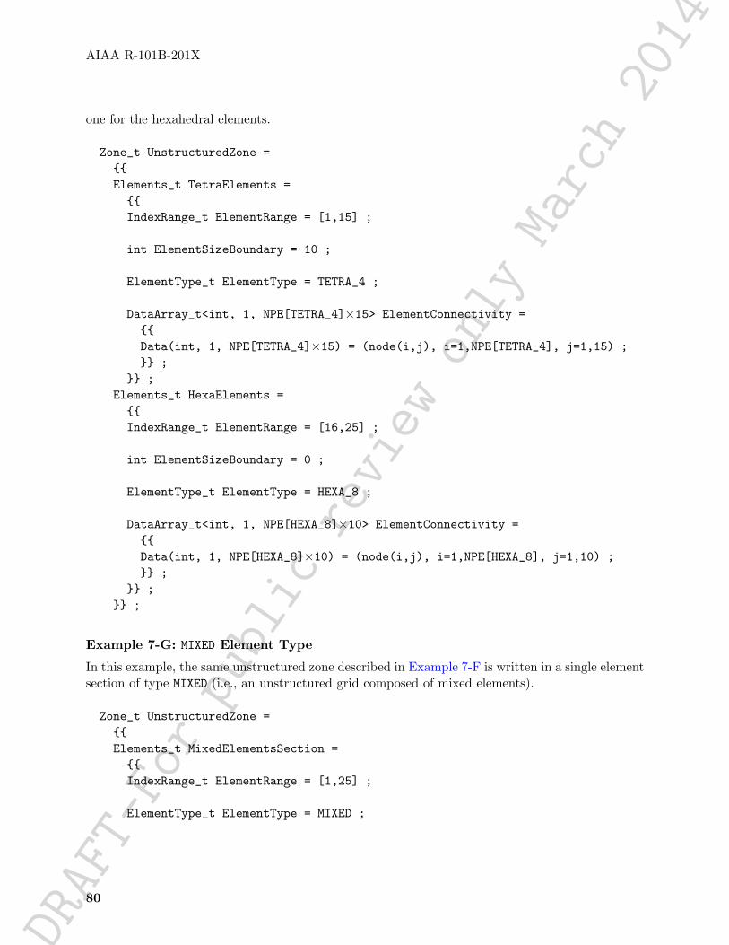
DRAFT-Forpublic

review

only


one for the hexahedral elements.

Zone_t UnstructuredZone ={{Elements_t TetraElements ={{IndexRange_t ElementRange = [1,15] ;

int ElementSizeBoundary = 10 ;

ElementType_t ElementType = TETRA_4 ;

DataArray_t<int, 1, NPE[TETRA_4]×15> ElementConnectivity ={{Data(int, 1, NPE[TETRA_4]×15) = (node(i,j), i=1,NPE[TETRA_4], j=1,15) ;}} ;

}} ;Elements_t HexaElements ={{IndexRange_t ElementRange = [16,25] ;

int ElementSizeBoundary = 0 ;

ElementType_t ElementType = HEXA_8 ;

DataArray_t<int, 1, NPE[HEXA_8]×10> ElementConnectivity ={{Data(int, 1, NPE[HEXA_8]×10) = (node(i,j), i=1,NPE[HEXA_8], j=1,10) ;}} ;

}} ;}} ;

Example 7-G: MIXED Element Type

In this example, the same unstructured zone described in Example 7-F is written in a single elementsection of type MIXED (i.e., an unstructured grid composed of mixed elements).

Zone_t UnstructuredZone ={{Elements_t MixedElementsSection ={{IndexRange_t ElementRange = [1,25] ;

ElementType_t ElementType = MIXED ;

80

DRAFT

-For

publ

icre

view

only

Mar

ch20

14

AIAA R-101B-201X

DataArray_t<int, 1, ElementDataSize> ElementConnectivity ={{Data(int, 1, ElementDataSize) = (etype(j),(node(i,j),

i=1,NPE[etype(j)]), j=1,25) ;}} ;

}} ;}} ;

7.5 Axisymmetry Structure Definition: Axisymmetry_t

The Axisymmetry_t data structure allows recording the axis of rotation and the angle of rotationaround this axis for a two-dimensional dataset that represents an axisymmetric database.

Axisymmetry_t :={List( Descriptor_t Descriptor1 ... DescriptorN ) ; (o)

DataArray_t<real,1,2> AxisymmetryReferencePoint ; (r)DataArray_t<real,1,2> AxisymmetryAxisVector ; (r)DataArray_t<real,1,1> AxisymmetryAngle ; (o)DataArray_t<char,2,[32,2]> CoordinateNames ; (o)




Notes

1. Default names for the Descriptor_t and UserDefinedData_t lists are as shown; users maychoose other legitimate names. Legitimate names must be unique within a given instance ofAxisymmetry_t and shall not include the names AxisymmetryAngle, AxisymmetryAxisVec-tor, AxisymmetryReferencePoint, CoordinateNames, DataClass, or DimensionalUnits.

2. AxisymmetryReferencePoint and AxisymmetryAxisVector are the required fields within theAxisymmetry_t structure.

AxisymmetryReferencePoint specifies the origin used for defining the axis of rotation.

AxisymmetryAxisVector contains the direction cosines of the axis of rotation, through the Ax-isymmetryReferencePoint. For example, for a 2-D dataset defined in the (x, y) plane, if Axisym-metryReferencePoint contains (0, 0) and AxisymmetryAxisVector contains (1, 0), the x-axis isthe axis of rotation.

81

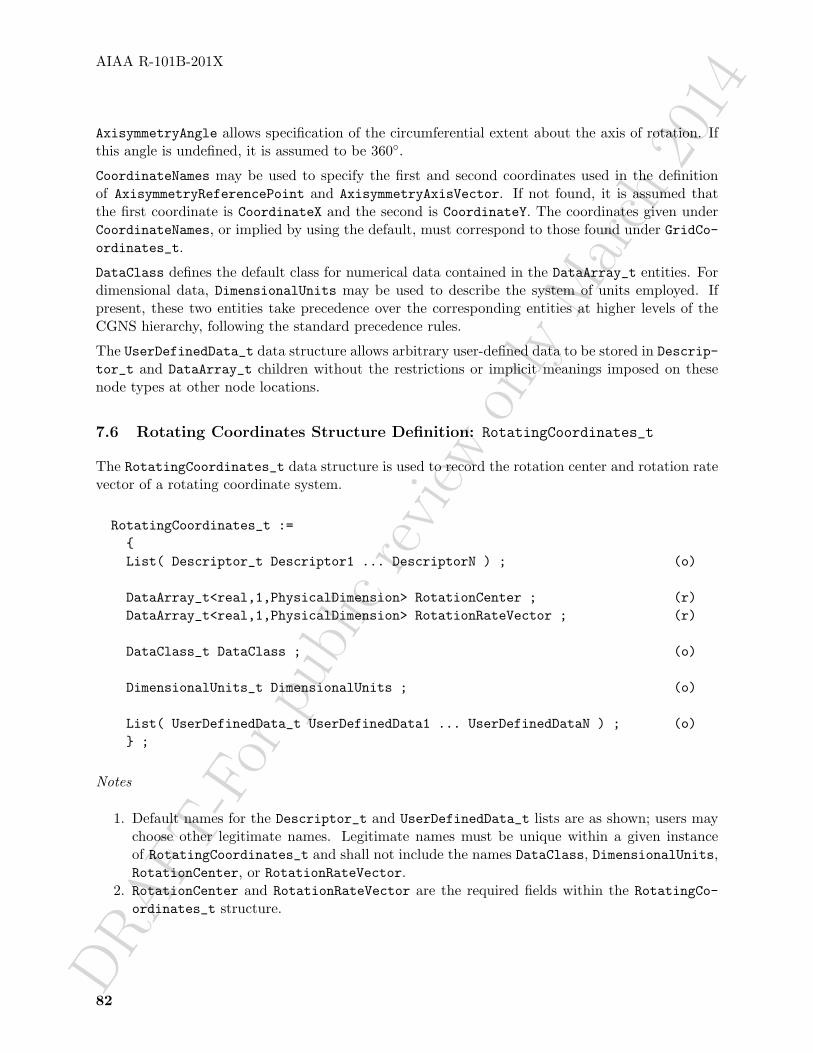
DRAFT

-For

publ

icre

view

only

Mar

ch20

14

AIAA R-101B-201X

AxisymmetryAngle allows specification of the circumferential extent about the axis of rotation. Ifthis angle is undefined, it is assumed to be 360◦.

CoordinateNames may be used to specify the first and second coordinates used in the definitionof AxisymmetryReferencePoint and AxisymmetryAxisVector. If not found, it is assumed thatthe first coordinate is CoordinateX and the second is CoordinateY. The coordinates given underCoordinateNames, or implied by using the default, must correspond to those found under GridCo-ordinates_t.

DataClass defines the default class for numerical data contained in the DataArray_t entities. Fordimensional data, DimensionalUnits may be used to describe the system of units employed. Ifpresent, these two entities take precedence over the corresponding entities at higher levels of theCGNS hierarchy, following the standard precedence rules.


7.6 Rotating Coordinates Structure Definition: RotatingCoordinates_t

The RotatingCoordinates_t data structure is used to record the rotation center and rotation ratevector of a rotating coordinate system.

RotatingCoordinates_t :={List( Descriptor_t Descriptor1 ... DescriptorN ) ; (o)

DataArray_t<real,1,PhysicalDimension> RotationCenter ; (r)DataArray_t<real,1,PhysicalDimension> RotationRateVector ; (r)




Notes

1. Default names for the Descriptor_t and UserDefinedData_t lists are as shown; users maychoose other legitimate names. Legitimate names must be unique within a given instanceof RotatingCoordinates_t and shall not include the names DataClass, DimensionalUnits,RotationCenter, or RotationRateVector.

2. RotationCenter and RotationRateVector are the required fields within the RotatingCo-ordinates_t structure.

82

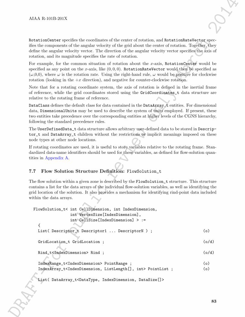
DRAFT-Forpublic

review

only


RotationCenter specifies the coordinates of the center of rotation, and RotationRateVector spec-ifies the components of the angular velocity of the grid about the center of rotation. Together, theydefine the angular velocity vector. The direction of the angular velocity vector specifies the axis ofrotation, and its magnitude specifies the rate of rotation.

For example, for the common situation of rotation about the x-axis, RotationCenter would bespecified as any point on the x-axis, like (0, 0, 0). RotationRateVector would then be specified as(ω,0,0), where ω is the rotation rate. Using the right-hand rule, ω would be positive for clockwiserotation (looking in the +x direction), and negative for counter-clockwise rotation.

Note that for a rotating coordinate system, the axis of rotation is defined in the inertial frameof reference, while the grid coordinates stored using the GridCoordinates_t data structure arerelative to the rotating frame of reference.

DataClass defines the default class for data contained in the DataArray_t entities. For dimensionaldata, DimensionalUnits may be used to describe the system of units employed. If present, thesetwo entities take precedence over the corresponding entities at higher levels of the CGNS hierarchy,following the standard precedence rules.


If rotating coordinates are used, it is useful to store variables relative to the rotating frame. Stan-dardized data-name identifiers should be used for these variables, as defined for flow-solution quan-tities in Appendix A.

7.7 Flow Solution Structure Definition: FlowSolution_t

The flow solution within a given zone is described by the FlowSolution_t structure. This structurecontains a list for the data arrays of the individual flow-solution variables, as well as identifying thegrid location of the solution. It also provides a mechanism for identifying rind-point data includedwithin the data arrays.

FlowSolution_t< int CellDimension, int IndexDimension,int VertexSize[IndexDimension],int CellSize[IndexDimension] > :=

{List( Descriptor_t Descriptor1 ... DescriptorN ) ; (o)

GridLocation_t GridLocation ; (o/d)


IndexRange_t<IndexDimension> PointRange ; (o)IndexArray_t<IndexDimension, ListLength[], int> PointList ; (o)

List( DataArray_t<DataType, IndexDimension, DataSize[]>

83

DRAFT

-For

publ

icre

view

only

Mar

ch20

14

AIAA R-101B-201X

DataArray1 ... DataArrayN ) ; (o)




Notes

1. Default names for the Descriptor_t, DataArray_t, and UserDefinedData_t lists are asshown; users may choose other legitimate names. Legitimate names must be unique within agiven instance of FlowSolution_t and shall not include the names DataClass, Dimension-alUnits, GridLocation, PointList, PointRange, or Rind.

2. There are no required fields for FlowSolution_t. GridLocation has a default of Vertex ifabsent. Rind also has a default if absent; the default is equivalent to having an instance ofRind whose RindPlanes array contains all zeros (see Section 4.8).

3. Both of the fields PointList and PointRange are optional. Only one of these two fields maybe specified.

4. The structure parameter DataType must be consistent with the data stored in the DataAr-ray_t structure entities (see Section 5.1); DataType is real for all flow-solution identifiersdefined in Appendix A.

5. For unstructured zones GridLocation options are limited to Vertex or CellCenter, unlessone of PointList or PointRange is present.

6. Indexing of data within the DataArray_t structures must be consistent with the associatednumbering of vertices or elements.

FlowSolution_t requires four structure parameters; CellDimension identifies the dimensionalityof cells or elements, IndexDimension identifies the dimensionality of the grid-size arrays, andVertexSize and CellSize are the number of core vertices and cells, respectively, in each indexdirection. For unstructured zones, IndexDimension is always 1.

The flow solution data is stored in the list of DataArray_t entities; each DataArray_t structureentity may contain a single component of the solution vector. Standardized data-name identifiersfor the flow-solution quantities are described in Appendix A. The field GridLocation specifies thelocation of the solution data with respect to the grid; if absent, the data is assumed to coincide withgrid vertices (i.e., GridLocation = Vertex). All data within a given instance of FlowSolution_tmust reside at the same grid location.

For structured grids, the value of GridLocation alone specifies the location and indexing of theflow solution data. Vertices are explicity indexed. Cell centers and face centers are indexed usingthe minimum of the connecting vertex indices, as described in the section Structured Grid Notationand Indexing Conventions (Section 3.2).

For unstructured grids, the value of GridLocation alone specifies location and indexing of flowsolution data only for vertex and cell-centered data. The reason for this is that element-based

84

DRAFT

-For

publ

icre

view

only

Mar

ch20

14

AIAA R-101B-201X

grid connectivity provided in the Elements_t data structures explicitly indexes only vertices andcells. For data stored at alternate grid locations (e.g. edges), additional connectivity information isneeded. This is provided by the optional fields PointRange and PointList; these refer to vertices,edges, faces or cell centers, depending on the values of CellDimension and GridLocation. Thefollowing table shows these relations.

CellDimension GridLocationVertex EdgeCenter *FaceCenter CellCenter

1 vertices − − cells (line elements)2 vertices edges − cells (area elements)3 vertices edges faces cells (volume elements)

In the table, *FaceCenter stands for the possible types: FaceCenter, IFaceCenter, JFaceCenteror KFaceCenter.

Although intended for edge or face-based solution data for unstructured grids, the fields PointRange/Listmay also be used to (redundantly) index vertex and cell-centered data. In all cases, indexing of flowsolution data corresponds to the element numbering as defined in the Elements_t data structures.

Rind is an optional field that indicates the number of rind planes (for structured grids) or rind pointsor elements (for unstructured grids) included in the data. Its purpose and function are identical tothose described in Section 7.1. Note, however, that the Rind in this structure is independent of theRind contained in GridCoordinates_t. They are not required to contain the same number of rindplanes or elements. Also, the location of any flow-solution rind points is assumed to be consistentwith the location of the core flow solution points (e.g., if GridLocation = CellCenter, rind pointsare assumed to be located at fictitious cell centers).

DataClass defines the default class for data contained in the DataArray_t entities. For dimensionalflow solution data, DimensionalUnits may be used to describe the system of units employed. Ifpresent these two entities take precedence over the corresponding entities at higher levels of theCGNS hierarchy. The rules for determining precedence of entities of this type are discussed inSection 6.4.


FUNCTION ListLength[]:

return value: intdependencies: PointRange, PointList

FlowSolution_t requires the structure function ListLength, which is used to specify the numberof entities (e.g. vertices) corresponding to a given PointRange or PointList. If PointRange isspecified, then ListLength is obtained from the number of points (inclusive) between the beginningand ending indices of PointRange. If PointList is specified, then ListLength is the number ofindices in the list of points. In this situation, ListLength becomes a user input along with theindices of the list PointList. By “user” we mean the application code that is generating the CGNSdatabase.

85

DRAFT

-For

publ

icre

view

only

Mar

ch20

14

AIAA R-101B-201X


return value: one-dimensional int array of length IndexDimensiondependencies: IndexDimension, VertexSize[], CellSize[], GridLocation, Rind, ListLength[]

The function DataSize[] is the size of flow solution data arrays. If Rind is absent then DataSizerepresents only the core points; it will be the same as VertexSize or CellSize depending onGridLocation. The definition of the function DataSize[] is as follows:

if (PointRange/PointList is present) then{DataSize[] = ListLength[] ;}

else if (Rind is absent) then{if (GridLocation = Vertex) or (GridLocation is absent){DataSize[] = VertexSize[] ;}

else if (GridLocation = CellCenter) then{DataSize[] = CellSize[] ;}

}else if (Rind is present) then{if (GridLocation = Vertex) or (GridLocation is absent) then{DataSize[] = VertexSize[] + [a + b,...] ;}

else if (GridLocation = CellCenter){DataSize[] = CellSize[] + [a + b,...] ;}

}

where RindPlanes = [a,b,...] (see Section 4.8 for the definition of RindPlanes).

7.8 Flow Solution Example

This section contains an example of the flow solution entity, including the designation of gridlocation and rind planes and data-normalization mechanisms.

Example 7-H: Flow Solution

Conservation-equation variables (ρ, ρu, ρv and ρe0) for a 2-D grid of size 11×5. The flowfield is cell-centered with two planes of rind data. The density, momentum and stagnation energy (ρe0) data is

86

DRAFT-Forpublic

review

only


nondimensionalized with respect to a freestream reference state whose quantities are dimensional.The freestream density and pressure are used for normalization; these values are 1.226 kg/m3 and1.0132×105 N/m2 (standard atmosphere conditions). The data-name identifier conventions for theconservation-equation variables are Density, MomentumX, MomentumY and EnergyStagnationDen-sity.

! CellDimension = 2! IndexDimension = 2! VertexSize = [11,5]! CellSize = [10,4]FlowSolution_t<2, [11,5], [10,4]> FlowExample ={{GridLocation_t GridLocation = CellCenter ;

Rind_t<2> Rind ={{int[4] RindPlanes = [2,2,2,2] ;}} ;

DataClass_t DataClass = NormalizedByDimensional ;

DimensionalUnits_t DimensionalUnits ={{MassUnits = Kilogram ;LengthUnits = Meter ;TimeUnits = Second ;TemperatureUnits = TemperatureUnitsNull ;AngleUnits = AngleUnitsNull ;}} ;

! DataType = real! Dimension = 2! DataSize = CellSize + [4,4] = [14,8]DataArray_t<real, 2, [14,8]> Density ={{Data(real, 2, [14,8]) = ((rho(i,j), i=-1,12), j=-1,6) ;

DataConversion_t DataConversion ={{ConversionScale = 1.226 ;ConversionOffset = 0 ;}} ;

DimensionalExponents_t DimensionalExponents ={{

87

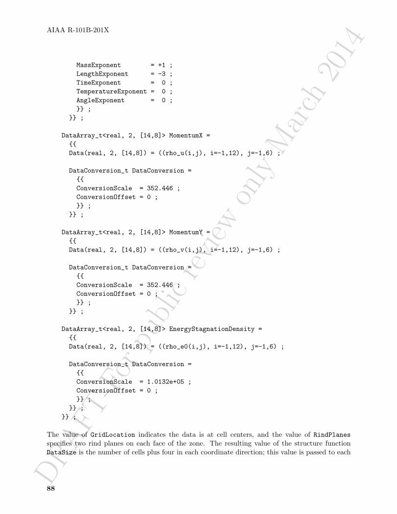
DRAFT

-For

publ

icre

view

only

Mar

ch20

14

AIAA R-101B-201X

MassExponent = +1 ;LengthExponent = -3 ;TimeExponent = 0 ;TemperatureExponent = 0 ;AngleExponent = 0 ;}} ;

}} ;

DataArray_t<real, 2, [14,8]> MomentumX ={{Data(real, 2, [14,8]) = ((rho_u(i,j), i=-1,12), j=-1,6) ;


}} ;

DataArray_t<real, 2, [14,8]> MomentumY ={{Data(real, 2, [14,8]) = ((rho_v(i,j), i=-1,12), j=-1,6) ;


}} ;

DataArray_t<real, 2, [14,8]> EnergyStagnationDensity ={{Data(real, 2, [14,8]) = ((rho_e0(i,j), i=-1,12), j=-1,6) ;

DataConversion_t DataConversion ={{ConversionScale = 1.0132e+05 ;ConversionOffset = 0 ;}} ;

}} ;}} ;

The value of GridLocation indicates the data is at cell centers, and the value of RindPlanesspecifies two rind planes on each face of the zone. The resulting value of the structure functionDataSize is the number of cells plus four in each coordinate direction; this value is passed to each

88

DRAFT-Forpublic

review

only


of the DataArray_t entities.

Since the data are all nondimensional and normalized by dimensional reference quantities, thisinformation is stated in DataClass and DimensionalUnits at the FlowSolution_t level ratherthan attaching the appropriate DataClass and DimensionalUnits to each DataArray_t entity. Itcould possibly be at even higher levels in the heirarchy. The contents of DataConversion are ineach case the denominator of the normalization; this is ρ∞ for density,

√p∞ρ∞ for momentum, and

p∞ for stagnation energy. The dimensional exponents are specified for density. For all the otherdata, the dimensional exponents are to be inferred from the data-name identifiers.

Note that no information is provided to identify the actual reference state or indicate that it isfreestream. This information is not needed for data manipulations involving renormalization orchanging the units of the converted raw data.

7.9 Zone Subregion Structure Definition: ZoneSubRegion_t

The ZoneSubRegion_t node allows for the ability to give flowfield or other information over a subsetof the entire zone in a CGNS file. This subset may be over a portion of a boundary, or it may beover a portion of the entire field.

ZoneSubRegion_t< int IndexDimension, int CellDimension > :={List( Descriptor_t Descriptor1 ... DescriptorN ) ; (o)List( Descriptor_t Descriptor1 ... DescriptorN ) ; (o)

int RegionCellDimension ; (o/d)


IndexRange_t<IndexDimension> PointRange ; (r:o:o:o)IndexArray_t<IndexDimension, ListLength, int> PointList ; (o:r:o:o)Descriptor_t BCRegionName ; (o:o:r:o)Descriptor_t GridConnectivityRegionName ; (o:o:o:r)

Rind_t<IndexDimension> Rind; (o/d)

List( DataArray_t<DataType, 1, ListLength[]>DataArray1 ... DataArrayN ) ; (o)





89

DRAFT

-For

publ

icre

view

only

Mar

ch20

14

AIAA R-101B-201X


Notes

1. Default names for the Descriptor_t, DataArray_t, and UserDefinedData_t lists are asshown; users may choose other legitimate names. Legitimate names must be unique within agiven instance of ZoneSubRegion_t and shall not include the names RegionCellDimension,Rind, PointRange, PointList, BCRegionName, GridConnectivityRegionName, FamilyName,DataClass or DimensionalUnits.

2. RegionCellDimension must be equal to or less than the cell dimension for the zone. If absent,then its default value is CellDimension.

3. GridLocation has a default value of Vertex if absent. Permissible values of GridLocationare determined by RegionCellDimension (see below). All data within a given instance ofZoneSubRegion_t must reside at the same grid location.

4. The extent of the region and distribution of its data is specified by one of PointRange,PointList, BCRegionName, or GridConnectivityRegionName. One and only one of thesemust be specified.

The extent of the subregion and the distribution of data within that subregion is determined byRegionCellDimension, GridLocation, and one of PointRange/List, BCRegionName, or GridCon-nectivityRegionName. For a 3-D subregion (RegionCellDimension = 3), data can be locatedat vertices, edges, face centers or cell centers. For a 2-D subregion (RegionCellDimension = 2),data can be located at vertices, edges or cell centers (i.e. area elements). It is anticipated that oneof the widest uses for ZoneSubRegion_t will be to store specific boundary-only information. Forexample, in a 3-D simulation, one may wish to store additional data on surfaces. In this case, theRegionCellDimension would be set to 2.

PointRange/List refer to vertices, edges, faces or cell centers, depending on the values of Re-gionCellDimension and GridLocation. Note that it is both the dimensionality of the zone(CellDimension) as well as the dimensionality of the subregion (RegionCellDimension), thatdetermines the types of elements permissible in PointRange/List. The following table shows theserelations.

CellDimension RegionCellDimension GridLocationVertex EdgeCenter *FaceCenter CellCenter

1 1 vertices − − cells (line elements)2 1 vertices edges − −2 2 vertices edges − cells (area elements)3 1 vertices edges − −3 2 vertices edges faces −3 3 vertices edges faces cells (volume elements)


90

DRAFT

-For

publ

icre

view

only

Mar

ch20

14

AIAA R-101B-201X

For both structured and unstructured grids, GridLocation = Vertex means that PointRange/Listrefers to vertex indices. For structured grids, edges, faces and cell centers are indexed using theminimum of the connecting vertex indices, as described in the section Structured Grid Notationand Indexing Conventions (Section 3.2). For unstructured grids, edges, faces and cell centers areindexed using their element numbering, as defined in the Elements_t data structures (Section 7.3).

If the vertices or elements of the subregion are continuously numbered, then PointRange maybe used. Otherwise, PointList should be used to list the vertices/elements. Alternatively, ifthe data locations and range of the subregion coincide with an existing BC region or zone-to-zone GridConnectivity region, then BCRegionName or GridConnectivityRegionName may be used.BCRegionName is a string giving the name of an existing BC_t node of the current zone. Grid-ConnectivityRegionName is a string giving the name of an existing GridConnectivity1to1_t orGridConnectivity_t node of the current zone. The name referred to should be unambiguous.

Consistent with FlowSolution_t, the subregion’s solution data is stored in the list of DataArray_tentities; each DataArray_t structure entity contains a single quantity. Standardized data-nameidentifiers for solution quantities are described in the section Conventions for Data-Name Identifiers(Appendix A). As noted above, all solution data within a given subregion must reside at the samegrid location.

DataClass defines the default class for data contained in the DataArray_t entities. For dimensionalflow solution data, DimensionalUnits may be used to describe the system of units employed. Ifpresent, these two entities take precedence over the corresponding entities at higher levels of theCGNS hierarchy, following the standard precedence rules (Section 6.4).

ZoneSubRegion_t requires the structure function ListLength[], which is used to specify the num-ber of data points (e.g. vertices, cell centers, face centers, edge centers) corresponding to the givenPointRange/List. If PointRange is specified, then ListLength is obtained from the number ofpoints (inclusive) between the beginning and ending indices of PointRange. If PointList is spec-ified, then ListLength is the number of indices in the list of points. In this situation, ListLengthbecomes a user input along with the indices of the list PointList. By “user” we mean the applica-tion code that is generating the CGNS database.

Rind is an optional field that indicates the number of rind planes (for structured grids) or rindpoints (for unstructured grids). If Rind is absent, then the DataArray_t structure entities containonly core data of length ListLength, as defined for this region. If Rind is present, it will provideinformation on the number of rind elements, in addition to the ListLength, that are containedin the DataArray_t structures. The bottom line is that Rind simply adds a specified number toListLength, as used by the DataArray_t structures.

The UserDefinedData_t data structure allows arbitrary user-defined data to be stored.

There may be multiple instances of ZoneSubRegion_t in a given zone. These may simply be multipleregions defined for a single solution, or they may be associated with different times / differentsolutions in a time-dependent simulation (in which case ZoneIterativeData (Section 11.1.2) shouldbe used to associate them).

91

DRAFT-Forpublic

review

only


7.10 Zone Subregion Examples

This section contains four examples of Zone Subregions, including the use of PointList, PointRangeand BCRegionName.

Example 7-I: Volume Subregion for a Structured Grid

For this example, it is assumed that a 1-zone 3-D structured grid exists of size (197×97×33). Insideof this zone, the user wishes to output a special subset region of interior data (say, temperatureand kinematic viscosity) at the specific cell-center locations i = 121-149, j = 17-45, k = 21-23.Even though this same data may possibly exist under FlowSolution_t (which holds the flowfielddata for the entire zone), this particular location may represent a special region of interest wherethe user wants to focus attention or output different types of flowfield variables or user-defineddata. Note that for structured grids, the location list always references grid nodes; in this case withGridLocation = Cellcenter the cell centers are indexed by the minimum i, j, and k indices of theconnecting vertices.

Under Zone_t:

ZoneSubRegion_t<3,3> Region1 ={{GridLocation_t GridLocation = CellCenter ;int RegionCellDimension = 3;IndexRange_t<3> PointRange ={{int[3] Begin = [121,17,21];int[3] End = [149,45,21];}};

! ListLength = (149-121+1)*(45-17+1)*(23-21+1) = 29*29*3 = 2523DataArray_t<real,1,2523> Temperature ={{Data(real,1,2523) = temperature at the cell centers specified}} ;

DataArray_t<real,1,2523> ViscosityKinematic ={{Data(real,1,2523) = kinematic viscosity at the cell centers specified}} ;

}} ; ! end Region1

Example 7-J: Volume Subregion for an Unstructured Grid

This example is like the previous one, except it is for an unstructured zone. Inside of this zone, theuser wishes to output a special subset region of data (say, temperature and kinematic viscosity)at a specific list of 2523 element cell-center locations, located somewhere within the (larger) fieldof elements. Recall that when GridLocation is anything other than Vertex in conjunction withunstructured grids, then the location list represents element numbers and not grid node numbers.

92

DRAFT-Forpublic

review

only


Under Zone_t:

ZoneSubRegion_t<1,3> Region1 ={{GridLocation_t GridLocation = CellCenter ;int RegionCellDimension = 3;IndexArray_t<1,2523,int> PointList ={{int[1] ElementList = list of 3-D element numbers where region data given}} ;

! ListLength = length of the element list = 2523DataArray_t<real,1,2523> Temperature ={{Data(real,1,2523) = temperature at the element cell centers specified}} ;

DataArray_t<real,1,2523> ViscosityKinematic ={{Data(real,1,2523) = kinematic viscosity at the element cell centers specified}} ;

}} ; ! end Region1

Example 7-K: Surface Subregion for an Unstructured Grid

In this example, boundary data is output on a 2-D surface subregion of a 3-D problem. Because thisis data on a topologically 2-D boundary (in a 3-D simulation), RegionCellDimension is set to 2.GridLocation is specified as FaceCenter. Recall that when GridLocation is anything other thanVertex in conjunction with unstructured grids, then the location list represents element numbersand not grid node numbers. Thus, the PointList/Range indicates particular surface elements (orboundary elements) that need to have been defined in the file under their own Elements_t node(s),separate from the 3-D volume elements that make up the grid. In this case, we assume that thesurface element numbers at which we are outputting data are 5568 through 5592 inclusive. Becausethe numbers occur in sequential order, we can make use of PointRange.

Under Zone_t:

ZoneSubRegion_t<1,3> Region1 ={{GridLocation_t GridLocation = FaceCenter ;int RegionCellDimension = 2;IndexArray_t<1,25,int> PointRange ={{int[1] Begin = [5568];int[1] End = [5592];}} ;

93

DRAFT

-For

publ

icre

view

only

Mar

ch20

14

AIAA R-101B-201X

! ListLength = length of the element list = 25DataArray_t<real,1,25> Temperature ={{Data(real,1,25) = temperature at the specific face element locations

specified}} ;

DataArray_t<real,1,25> ViscosityKinematic ={{Data(real,1,25) = kinematic viscosity at the specific face element

locations specified}} ;

}} ; ! end Region1

Example 7-L: Surface Subregion Utilizing BC Information

In this example, boundary data is output at the same locations where the BCs are specified ina particular BC_t node (in this case the ListLength is 25). Note that because this is data on atopologically 2-D boundary (in a 3-D simulation), RegionCellDimension is set to 2. GridLocationis not specified, because it is inherited from the BC_t node along with the ListLength.

Under Zone_t:

ZoneSubRegion_t<1,3> Region1 ={{int RegionCellDimension = 2;Descriptor_t BCRegionName = "name of a ZoneBC/BC_t node" ;

! ListLength = length of the point/element list from BC_t = 25DataArray_t<real,1,25> Temperature ={{Data(real,1,25) = temperature at the specific BC locations

specified}} ;

DataArray_t<real,1,25> ViscosityKinematic ={{Data(real,1,25) = kinematic viscosity at the specific BC

locations specified}} ;

}} ; ! end Region1

94

DRAFT-Forpublic

review

only


8 Multizone Interface Connectivity

This section defines structures for describing multizone interface connectivity for 1-to-1 abutting,mismatched abutting, and overset type interfaces. The different types of zone interfaces are de-scribed in Section 3.4. All interface connectivity information pertaining to a given zone is groupedtogether in a ZoneGridConnectivity_t structure entity; this in turn is contained in a zone struc-ture entity (see the definition of Zone_t in Section 6.3).

Before presentation of the structure definitions, a few design features require comment. All indicesused to describe interfaces are the dimensionality (IndexDimension) of the grid, even when theyare used to describe lower-dimensional zonal boundaries for abutting interfaces. The alternativefor structured zones that was not chosen is to use lower-dimensional indices for lower-dimensionalinterfaces (e.g., for a 3-D grid, use two-dimensional indices for describing grid planes that areinterfaces). Both alternatives offer trade-offs. The lower-dimensional indices require cyclic notationconventions and additional identification of face location; whereas, full-dimensional indices resultin one redundant index component when describing points along a grid plane. We decided thatfull-dimensional indices would be more usable and less error prone in actual implementation.

A major consequence of this decision is that connectivity information for describing mismatchedabutting interfaces and overset interfaces can be merged into a single structure, GridConnectiv-ity_t (see Section 8.4 below). In fact, this single structure type can be used to describe all zonalinterfaces.

A second design choice was to duplicate all 1-to-1 abutting interface information within the CGNSdatabase. It is possible to describe a given 1-to-1 interface with a single set of connectivity data.In contrast, mismatched and overset interfaces require different connectivity information when theroles of receiver and donor zones are interchanged. Therefore, a given mismatched or oversetinterface requires two sets of connectivity data within the database. The decision to force two setsof connectivity data (one contained in each of the Zone_t entities for the two adjacent zones) foreach 1-to-1 interface makes the connectivity structures for all interface types look and functionsimilarly. It also fits better with the zone-by-zone hierarchy chosen for the CGNS database. Theminor penalty in data duplication was deemed worth the advantages gained.

Note that it is a CGNS design intent that a given zone boundary segment or location should atmost be defined (or covered) by either a boundary condition or a multizone interface connectivity,but not by both.

8.1 Zonal Connectivity Structure Definition: ZoneGridConnectivity_t

All multizone interface grid connectivity information pertaining to a given zone is contained inthe ZoneGridConnectivity_t structure. This includes abutting interfaces (1-to-1 and generalmismatched), overset-grid interfaces, and overset-grid holes.

ZoneGridConnectivity_t< int IndexDimension, int CellDimension > :={List( Descriptor_t Descriptor1 ... DescriptorN ) ; (o)

95

DRAFT-Forpublic

review

only


List( GridConnectivity1to1_t<IndexDimension>GridConnectivity1to11 ... GridConnectivity1to1N ) ; (o)

List( GridConnectivity_t<IndexDimension, CellDimension>GridConnectivity1 ... GridConnectivityN ) ; (o)

List( OversetHoles_t<IndexDimension>OversetHoles1 ... OversetHolesN ) ; (o)


Notes

1. Default names for the Descriptor_t, GridConnectivity1to1_t, GridConnectivity_t, Over-setHoles_t, and UserDefinedData_t lists are as shown; users may choose other legitimatenames. Legitimate names must be unique within a given instance of ZoneGridConnectivity_t.

2. All lists within the ZoneGridConnectivity_t structure may be empty.

ZoneGridConnectivity_t requires two structure parameters, IndexDimension, which is passedonto all connectivity substructures, and CellDimension, which is passed to GridConnectivity_tonly.

Connectivity information for 1-to-1 or matched multizone interfaces is contained in the GridCon-nectivity1to1_t structure. Abutting and overset connectivity is contained in the GridConnec-tivity_t structure, and overset-grid holes are identified in the OversetHoles_t structure.


8.2 1-to-1 Interface Connectivity Structure Definition: GridConnectivity1to1_t

GridConnectivity1to1_t only applies to structured zones interfacing with structured donors andwhose interface is a logically rectangular region. It contains connectivity information for a multizoneinterface patch that is abutting with 1-to-1 matching between adjacent zone indices (also referredto as C0 connectivity). An interface patch is the subrange of the face of a zone that touches oneand only one other zone. This structure identifies the subrange of indices for the two adjacent zonesthat make up the interface and gives an index transformation from one zone to the other. It alsoidentifies the name of the adjacent zone.

All the interface patches for a given zone are contained in the ZoneGridConnectivity_t entityfor that zone. If a face of a zone touches several other zones (say N), then N different instancesof the GridConnectivity1to1_t structure must be included in the zone to describe each separateinterface patch. This convention requires that a single interface patch be described twice in thedatabase—once for each adjacent zone.

96

DRAFT-Forpublic

review

only


GridConnectivity1to1_t< int IndexDimension > :={List( Descriptor_t Descriptor1 ... DescriptorN ) ; (o)

int[IndexDimension] Transform ; (o/d)

IndexRange_t<IndexDimension> PointRange ; (r)IndexRange_t<IndexDimension> PointRangeDonor ; (r)

Identifier(Zone_t) ZoneDonorName ; (r)

GridConnectivityProperty_t GridConnectivityProperty ; (o)



Notes

1. Default names for the Descriptor_t and UserDefinedData_t lists are as shown; users maychoose other legitimate names. Legitimate names must be unique within a given instanceof GridConnectivity1to1_t and shall not include the names GridConnectivityProperty,PointRange, PointRangeDonor, Transform, or Ordinal.

2. If Transform is absent, then its default value is [+1,+2,+3].3. ZoneDonorName must be equated to a zone identifier within the current CGNS database (i.e.,

it must be equal to one of the Zone_t identifiers contained in the current CGNSBase_t entity).4. Beginning indices of PointRange and PointRangeDonor must coincide (i.e., must be the same

physical point); ending indices of PointRange and PointRangeDonor must also coincide.5. Elements of Transform must be signed integers in the range -IndexDimension, . . ., +In-

dexDimension; element magnitudes may not be repeated. In 3-D allowed elements are 0, ±1,±2, ±3.

PointRange contains the subrange of indices that makes up the interface patch in the currentzone (i.e., that Zone_t entity that contains the given instance of GridConnectivity1to1_t).PointRangeDonor contains the interface patch subrange of indices for the adjacent zone (whoseidentifier is given by ZoneDonorName). By convention the indices contained in PointRange andPointRangeDonor refer to vertices.

Transform contains a short-hand notation for the transformation matrix describing the relation be-tween indices of the two adjacent zones. The transformation matrix itself has rank IndexDimensionand contains elements +1, −1 and 0; it is orthonormal and its inverse is its transpose. The trans-formation matrix (T) works as follows: if Index1 and Index2 are the indices of a given point onthe interface, where Index1 is in the current zone and Index2 is in the adjacent zone, then theirrelationship is,

97

DRAFT

-For

publ

icre

view

only

Mar

ch20

14

AIAA R-101B-201X

Index2 = T.(Index1 - Begin1) + Begin2

Index1 = Transpose[T].(Index2 - Begin2) + Begin1

where the “.” notation indicates matrix-vector multiply. Begin1 and End1 are the subrange indicescontained in PointRange, and Begin2 and End2 are the subrange indices contained in PointRange-Donor.

The short-hand notation used in Transform is as follows: each element shows the image in theadjacent zone’s face of a positive index increment in the current zone’s face. The first elementis the image of a positive increment in i; the second element is the image of an increment in j;and the third (in 3-D) is the image of an increment in k on the current zone’s face. For 3-D, thetransformation matrix T is constructed from Transform = [±a, ±b, ±c] as follows:

T =

sgn(a) del(a− 1) sgn(b) del(b− 1) sgn(c) del(c− 1)sgn(a) del(a− 2) sgn(b) del(b− 2) sgn(c) del(c− 2)sgn(a) del(a− 3) sgn(b) del(b− 3) sgn(c) del(c− 3)

,where,

sgn(x) ≡{

+1, if x ≥ 0−1, if x < 0

del(x− y) ≡{

1, if abs(x) = abs(y)0, otherwise

For example, Transform = [−2, +3, +1] gives the transformation matrix,

T =

0 0 +1−1 0 0

0 +1 0

.For establishing relationships between adjacent and current zone indices lying on the interface itself,one of the elements of Transform is superfluous since one component of both interface indicesremains constant. It is therefore acceptable to set that element of Transform to zero.

If the transformation matrix is used for continuation of computational coordinates into the adjacentzone (e.g., to find the location of a rind point in the adjacent zone), then all elements of Transformare needed. If the above mentioned superfluous element is set to zero, it can be easily regeneratedfrom PointRange and PointRangeDonor and the grid sizes of the two zones. This is done bydetermining the faces represented by PointRange and PointRangeDonor (i.e., i-min, i-max, j-min,etc.). If one is a minimum face and the other a maximum face, then the sign of the missing elementin Transform is “+”, and the value of the missing element in the transformation matrix (T) is+1. If the faces are both minimums or are both maximums, the sign is “−”. Next, the positionand magnitude of the element in Transform, and hence the row and column in the transformationmatrix, is given by the combinations of i, j and k faces for the two. For example, if PointRangerepresents a j-min or j-max face and PointRangeDonor represents an i-min or i-max face, thenthe missing element’s position in Transform is 2 and its magnitude is 1 (i.e., Transform = [∗, ±1,∗]).

Note also that the transform matrix and the two index pairs overspecify the interface patch. Forexample, End2 can be obtained from Transform, Begin1, End1 and Begin2.

98

DRAFT-Forpublic

review

only


A GridConnectivityProperty_t data structure, described in Section 8.6, may be used to recordspecial properties associated with particular connectivity patches, such as a periodic interface, oran interface where data is to be averaged in some way.


Ordinal is user-defined and has no restrictions on the values that it can contain. It is included forbackward compatibility to assist implementation of the CGNS system into applications whose I/Odepends heavily on the numbering of zone interfaces. Since there are no restrictions on the valuescontained in Ordinal (or that Ordinal is even provided), there is no guarantee that the interfacesin an existing CGNS database will have sequential values from 1 to N without holes or repetitions.Use of Ordinal is discouraged and is on a user-beware basis.

8.3 1-to-1 Interface Connectivity Examples

This section contains two examples of structure entities for describing the connectivity for struc-tured-zone 1-to-1 abutting multizone interfaces. Appendix B contains additional examples of 1-to-1interfaces.

Example 8-A: 1-to-1 Abutting of Complete Faces

Two zones have the same orientation; zone 1 is 9×17×11 and zone 2 is 9×17×21. The k-maxface of zone 1 abuts the k-min face of zone 2. Contained in the structure entities of zone 1 is thefollowing interface structure:

GridConnectivity1to1_t<3> Zone1/ZoneGridConnectivity/KMax ={{int[3] Transform = [1,2,3] ;IndexRange_t<3> PointRange ={{int[3] Begin = [1,1,11] ;int[3] End = [9,17,11] ;}} ;

IndexRange_t<3> PointRangeDonor ={{int[3] Begin = [1,1,1] ;int[3] End = [9,17,1] ;}} ;

Identifier(Zone_t) ZoneDonorName = Zone2 ;}} ;

Contained in the structure entities of zone 2 is the following:

GridConnectivity1to1_t<3> Zone2/ZoneGridConnectivity/KMin ={{

99

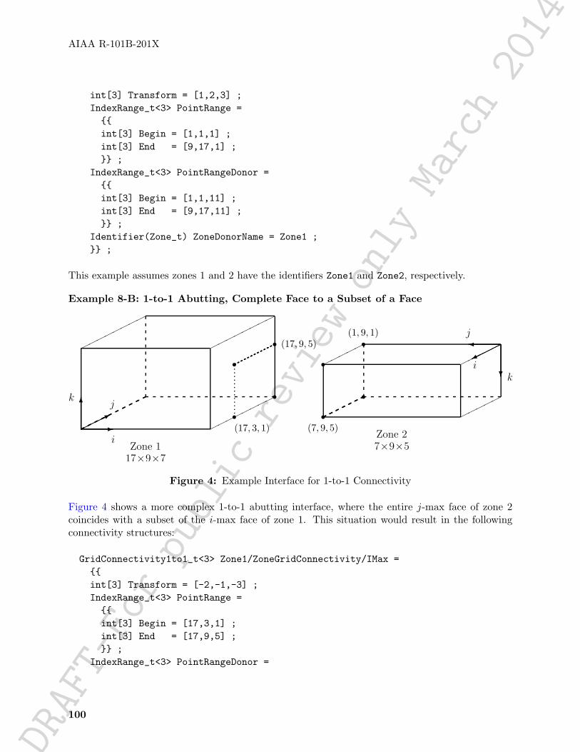
DRAFT-Forpublic

review

only


int[3] Transform = [1,2,3] ;IndexRange_t<3> PointRange ={{int[3] Begin = [1,1,1] ;int[3] End = [9,17,1] ;}} ;



This example assumes zones 1 and 2 have the identifiers Zone1 and Zone2, respectively.

Example 8-B: 1-to-1 Abutting, Complete Face to a Subset of a Face

��

��s

ss

s-��*

6

i

jk

(17, 3, 1)

(17, 9, 5)

Zone 117×9×7

��

��s

ss

s

��

�

?i

j

k

(7, 9, 5)

(1, 9, 1)

Zone 27×9×5

Figure 4: Example Interface for 1-to-1 Connectivity

Figure 4 shows a more complex 1-to-1 abutting interface, where the entire j-max face of zone 2coincides with a subset of the i-max face of zone 1. This situation would result in the followingconnectivity structures:

GridConnectivity1to1_t<3> Zone1/ZoneGridConnectivity/IMax ={{int[3] Transform = [-2,-1,-3] ;IndexRange_t<3> PointRange ={{int[3] Begin = [17,3,1] ;int[3] End = [17,9,5] ;}} ;

IndexRange_t<3> PointRangeDonor =

100

DRAFT

-For

publ

icre

view

only

Mar

ch20

14

AIAA R-101B-201X

{{int[3] Begin = [7,9,5] ;int[3] End = [1,9,1] ;}} ;


GridConnectivity1to1_t<3> Zone2/ZoneGridConnectivity/JMax ={{int[3] Transform = [-2,-1,-3] ;IndexRange_t<3> PointRange ={{int[3] Begin = [1,9,1] ;int[3] End = [7,9,5] ;}} ;



This example also assumes zones 1 and 2 have the identifiers Zone1 and Zone2, respectively. Notethat the index transformation matrix for both this and the previous examples is symmetric; hence,the value of Transform is identical for both members of the interface pair. In general this will notalways be the case.

8.4 General Interface Connectivity Structure Definition: GridConnectivity_t

GridConnectivity_t contains connectivity information for generalized multizone interfaces, andmay be used for any mix of structured and unstructured zones. Its purpose is to describe mismatched-abutting and overset interfaces, but can also be used for 1-to-1 abutting interfaces.

For abutting interfaces that are not 1-to-1, also referred to as patched or mismatched, an interfacepatch is the subrange of the face of a zone that touches one and only one other zone. Thisstructure identifies the subrange of indices (or array of indices) that make up the interface andgives their image in the adjacent (donor) zone. It also identifies the name of the adjacent zone.If a given face of a zone touches several (say N) adjacent zones, then N different instances ofGridConnectivity_t are needed to describe all the interfaces. For a single abutting interface, twoinstances of GridConnectivity_t are needed in the database – one for each adjacent zone.

For overset interfaces, this structure identifies the fringe points of a given zone that lie in one andonly one other zone. If the fringe points of a zone lie in several (say N) overlapping zones, thenN different instances of GridConnectivity_t are needed to describe the overlaps. It is possiblewith overset grids that a single fringe point may actually lie in several overlapping zones (though in

101

DRAFT

-For

publ

icre

view

only

Mar

ch20

14

AIAA R-101B-201X

typical usage, linkage to only one of the overlapping zones is kept). There is no restriction againsta given fringe point being contained within multiple instances of GridConnectivity_t; therefore,this structure allows the description of a single fringe point lying in several overlapping zones.

GridConnectivityType_t := Enumeration(GridConnectivityTypeNull,GridConnectivityTypeUserDefined,Overset,Abutting,Abutting1to1 ) ;

GridConnectivity_t< int IndexDimension, int CellDimension > :={List( Descriptor_t Descriptor1 ... DescriptorN ) ; (o)

GridConnectivityType_t GridConnectivityType ; (o/d)


IndexRange_t<IndexDimension> PointRange ; (o:r)IndexArray_t<IndexDimension, PointListSize, int> PointList ; (r:o)IndexArray_t<IndexDimension, PointListSize, int> PointListDonor ; (o)IndexArray_t<IndexDimension, PointListSize, int> CellListDonor ; (o)

Identifier(Zone_t) ZoneDonorName ; (r)

DataArray_t <real, 2, [CellDimension, PointListSize]> InterpolantsDonor (o)

GridConnectivityProperty_t GridConnectivityProperty ; (o)



Notes

1. Default names for the Descriptor_t and UserDefinedData_t lists are as shown; usersmay choose other legitimate names. Legitimate names must be unique within a given in-stance of GridConnectivity_t and shall not include the names CellListDonor, GridCon-nectivityProperty, GridConnectivityType, GridLocation, InterpolantsDonor, Ordi-nal, PointList, PointListDonor, or PointRange.

2. ZoneDonorName must be equated to a zone identifier within the current CGNS database (i.e.,it must be equal to one of the Zone_t identifiers contained in the current CGNSBase_t entity).

3. If GridConnectivityType is absent, then its default value is Overset.

102

DRAFT

-For

publ

icre

view

only

Mar

ch20

14

AIAA R-101B-201X

4. For Abutting or Abutting1to1 interfaces, GridLocation can be either Vertex or FaceCen-ter. When GridLocation is set to Vertex, then PointList or PointRange refer to nodeindices, for both structured and unstructured grids. When GridLocation is set to FaceCen-ter, then PointList or PointRange refer to face elements. Face elements are indexed usingdifferent methods depending if the zone is structured or unstructured. For a structured zone,face elements are indexed using the minimum of the connecting vertex indices, as describedin Section 3.2. For an unstructured zone, face elements are indexed using their element num-bering, as defined in the Elements_t data structures. For Overset interfaces, GridLocationcan be either Vertex or CellCenter, allowing the description of the overlap region in thereceiver zone to be consistent with the grid location used for storing the flow solution. IfGridLocation is absent, then its default value is Vertex.

5. One of PointRange and PointList must be specified, but not both.6. If PointRange is specified, then an index ordering convention is needed to map receiver-zone

grid points to donor-zone grid points. FORTRAN multidimensional array ordering is used.7. If GridConnectivityType is Abutting1to1 or Abutting, then PointRange or PointList

must define points associated with a face subrange (if the zone is structured, all points mustbe in a single computational grid plane); the donor-zone grid locations defined by PointList-Donor or CellListDonor must also be associated with a face subrange.

8. If donor information is given, either PointListDonor alone, or CellListDonor with or with-out InterpolantsDonor, must be used. The use of PointListDonor is restricted to Abut-ting1to1, whereas CellListDonor can be used for any interface type.

9. Thus, for a GridConnectivityType that is not Abutting1to1, there are three allowable lev-els of description concerning the connectivity information: (a) full, giving ZoneDonorNamewith CellListDonor plus InterpolantsDonor; (b) partial, giving ZoneDonorName with Cel-lListDonor but no InterpolantsDonor; or (c) minimal, giving ZoneDonorName only.

The type of multizone interface connectivity may be Overset, Abutting, or Abutting1to1. Over-set refers to zones that overlap; for a 3-D configuration the overlap is a 3-D region. Abutting refersto zones that abut or touch, but do not overlap (other than the vertices and faces that make upthe interface). Abutting1to1 is a special case of abutting interfaces where grid lines are continuousacross the interface and all vertices on the interface are shared by the two adjacent zones. SeeSection 3.4 for a description of the three different types of interfaces.

The interface grid points within the receiver zone may be specified by PointRange if they constitutea logically rectangular region (e.g., an abutting interface where an entire face of the receiver zoneabuts with a part of a face of the donor zone). In all other cases, PointList should be used to listthe receiver-zone grid points making up the interface. For a structured-to-structured interface, allindices in PointRange or PointList should have one index element in common (see note 7).

GridLocation identifies the location of indices within the receiver zone described by PointRange orPointList. It also identifies the location of indices defined by PointListDonor in the donor zone.GridLocation does not apply to CellListDonor or InterpolantsDonor. The CellListDonor isalways an index or indices that define a particular cell or element, while the InterpolantsDonordefines an interpolation value relative to the cell/element vertices. In other words, when usingInterpolantsDonor, the interpolants are always given with respect to the vertices of the donor zone.InterpolantsDonor is currently only defined for structured grids and certain basic unstructured

103

DRAFT

-For

publ

icre

view

only

Mar

ch20

14

AIAA R-101B-201X

grid element types.

For structured grids, the interpolant value is given along each index direction, depending on thelocation within the cell. For example, if the point is located within the cell at a position 75% in thei-direction, 41% in the j-direction, and 20% in the k-direction, then InterpolantsDonor values (r,s, t) would be (0.75, 0.41, 0.20).

The interpolation function is a linear combination of the x, y, and z values at the surroundingnodes:

d =N∑i=1

Wi · di

where d is the x, y, or z value at an interior point in the cell, di is the x, y, or z value at nodei, and Wi is a weight at node i. The weights are functions of the parametric variables r, s, and t(corresponding with the i, j, and k directions, respectively), which vary from 0 to 1, inclusively.For structured grids in 3-D, N = 8. Note that for skewed, non-parallel grids, it is not always easyto determine the interpolants geometrically, and it may be necessary to solve an inverse problemusing the interpolation function.

��

��

��

��

��

�

6

�

��

i, j, k

i + 1, j, k

i + 1, j, k + 1i + 1, j + 1, k + 1

i, j + 1, k

i + 1, j + 1, k

r

t

s

Wi,j,k = (1− r)(1− s)(1− t)Wi+1,j,k = r(1− s)(1− t)Wi,j+1,k = (1− r)s(1− t)Wi,j,k+1 = (1− r)(1− s)t

Wi+1,j+1,k = rs(1− t)Wi+1,j,k+1 = r(1− s)tWi,j+1,k+1 = (1− r)st

Wi+1,j+1,k+1 = rst

For unstructured grids, InterpolantsDonor is defined only for the basic linear element types:BAR_2, TRI_3, QUAD_4, TETRA_4, PYRA_5, PENTA_6, and HEXA_8, defined in Section 3.3. The direc-tionality for the r, s, and t interpolants for the basic element types is defined as follows.

BAR_2

s s -1 2

rW1 = 1− rW2 = r

104

DRAFT

-For

publ

icre

view

only

Mar

ch20

14

AIAA R-101B-201X

TRI_3

��

��

��

��Z

ZZ

ZZ

ZZ

Z

s

ss ��

�>Z

ZZ}

1

23

rs W1 = 1− r − sW2 = r

W3 = s

QUAD_4

s

ss

s

�

�1

2

3

4

r

s

W1 = (1− r)(1− s)W2 = r(1− s)W3 = rs

W4 = (1− r)s

TETRA_4

QQ

QQ

QQ

QQ

Q��

��

��

�l

ll

ll

ll

l��

��

��

��s

s

s

s

QQ

QQs

:

��

1

2

3

4

r

s

t W1 = 1− r − s− tW2 = r

W3 = s

W4 = t

105

DRAFT

-For

publ

icre

view

only

Mar

ch20

14

AIAA R-101B-201X

PYRA_5

,,

,,

,,

,,

,,

,TTTTTTT(((((((((((B

BBBBBBBBBBBBBB�

��

��

��

��

��

��

��

�s s

ss

s

((((:

AA

AK

��

12

3

4

5

r

s

tW1 = (1− r)(1− s)(1− t)W2 = r(1− s)(1− t)W3 = rs(1− t)W4 = (1− r)s(1− t)W5 = t

PENTA_6

��

��

��

��Z

ZZ

ZZ

ZZ

Z

s s

s

s s

s

-

��

�>

6

1 2

3

4 5

6

r

s

t

W1 = (1− r − s)(1− t)W2 = r(1− t)W3 = s(1− t)W4 = (1− r − s)tW5 = rt

W6 = st

106

DRAFT

-For

publ

icre

view

only

Mar

ch20

14

AIAA R-101B-201X

HEXA_8

��

��

��

��

��

�

sss

s

sss

s6

�

��

1

23

4

5

67

8

r

t

s

W1 = (1− r)(1− s)(1− t)W2 = r(1− s)(1− t)W3 = rs(1− t)W4 = (1− r)s(1− t)W5 = (1− r)(1− s)tW6 = r(1− s)tW7 = rst

W8 = (1− r)st

PointListDonor may only be used when the interface is Abutting1to1. It contains the imagesof all the receiver-zone interface points in the donor zone. If the zone is structured, all indices inPointListDonor should have one index element in common.

For mismatched or overset interfaces, the zone connectivity donor information, when given, isdefined using either the CellListDonor alone, or the combination of CellListDonor and Inter-polantsDonor. CellListDonor contains the list of donor cells or elements in which each node ofthe receiver zone can be located. InterpolantsDonor contains the interpolation factors to locatethe receiver nodes in the donor cells. InterpolantsDonor may be thought of as bi- or tri-linearinterpolants (depending on CellDimension) in the cell of the donor zone.

A GridConnectivityProperty_t data structure, described in Section 8.6, may be used to recordspecial properties associated with particular connectivity patches, such as a periodic interface, oran interface where data is to be averaged in some way.


Ordinal is user-defined and has no restrictions on the values that it can contain. It is included forbackward compatibility to assist implementation of the CGNS system into applications whose I/Odepends heavily on the numbering of zone interfaces. Since there are no restrictions on the valuescontained in Ordinal (or that Ordinal is even provided), there is no guarantee that the interfacesfor a given zone in an existing CGNS database will have sequential values from 1 to N withoutholes or repetitions. Use of Ordinal is discouraged and is on a user-beware basis.

FUNCTION PointListSize:


107

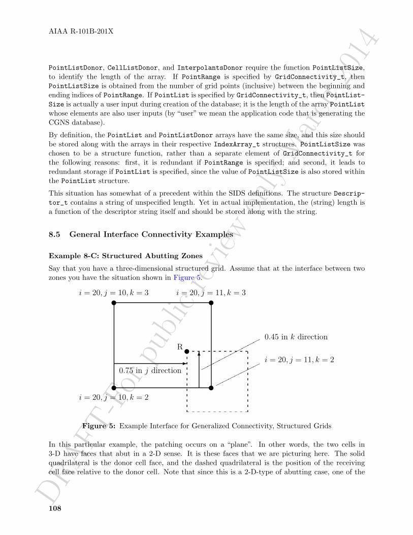
DRAFT

-For

publ

icre

view

only

Mar

ch20

14

AIAA R-101B-201X

PointListDonor, CellListDonor, and InterpolantsDonor require the function PointListSize,to identify the length of the array. If PointRange is specified by GridConnectivity_t, thenPointListSize is obtained from the number of grid points (inclusive) between the beginning andending indices of PointRange. If PointList is specified by GridConnectivity_t, then PointList-Size is actually a user input during creation of the database; it is the length of the array PointListwhose elements are also user inputs (by “user” we mean the application code that is generating theCGNS database).

By definition, the PointList and PointListDonor arrays have the same size, and this size shouldbe stored along with the arrays in their respective IndexArray_t structures. PointListSize waschosen to be a structure function, rather than a separate element of GridConnectivity_t forthe following reasons: first, it is redundant if PointRange is specified; and second, it leads toredundant storage if PointList is specified, since the value of PointListSize is also stored withinthe PointList structure.

This situation has somewhat of a precedent within the SIDS definitions. The structure Descrip-tor_t contains a string of unspecified length. Yet in actual implementation, the (string) length isa function of the descriptor string itself and should be stored along with the string.

8.5 General Interface Connectivity Examples

Example 8-C: Structured Abutting Zones

Say that you have a three-dimensional structured grid. Assume that at the interface between twozones you have the situation shown in Figure 5.

v v

vv

v-

6

0.75 in j direction �� 0.45 in k direction

i = 20, j = 10, k = 2

i = 20, j = 10, k = 3 i = 20, j = 11, k = 3

��i = 20, j = 11, k = 2

R

Figure 5: Example Interface for Generalized Connectivity, Structured Grids

In this particular example, the patching occurs on a “plane”. In other words, the two cells in3-D have faces that abut in a 2-D sense. It is these faces that we are picturing here. The solidquadrilateral is the donor cell face, and the dashed quadrilateral is the position of the receivingcell face relative to the donor cell. Note that since this is a 2-D-type of abutting case, one of the

108

DRAFT-Forpublic

review

only


indices (in this case i = 20, which represents imax) of the donor cell is constant. For this example,the point R of the receiver cell is located within the donor cell pictured, and we wish to give theCellListDonor and InterpolantsDonor for it.

Because this is a structured grid, the CellListDonor in this case is given by

CellListDonor = (19, 10, 2)

Here, we are using the “Structured Grid Notation and Indexing Conventions” (see Section 3.2) thatsay cell centers, face centers, and edge centers are indexed by the minimum i, j, and k indices ofthe connecting vertices.

The InterpolantsDonor defines an interpolation value relative to the cell/element vertices. In thiscase, say that the point R is located 0.75 along the j-index direction and 0.45 along the k-indexdirection. (It also lies on the i = 20, or imax face.) Thus, in this example:

InterpolantsDonor = (1.0, 0.75, 0.45)

Note that if the donor zone was instead located on an i = 1 (imin face), then the CellListDonorwould be (1, 10, 2) and the InterpolantsDonor would be (0.0, 0.75, 0.45).

Example 8-D: Unstructured Abutting Zones, HEXA_8 Donor Cell

As a second example, assume that you have the same setup as before, but now with a three-dimensional unstructured grid, shown in Figure 6. In this case, we no longer have a 3-D array ofindices defining coordinate directions. Instead, we simply have a 1-D list of indices as well as a listof volume (and possibly face) elements composed of those indices. In this example we again areassuming the two zones abut in a 2-D sense. We now have the choice of describing the donor interms of its volume element or its boundary (face) element, if available. Here in this example, weuse the volume element.

The HEXA_8 volume element has been appropriately numbered, using the “Unstructured Grid Ele-ment Numbering Conventions” defined in Section 3.3. In this example, it is the 1-2-3-4 face of thevolumetric element that is abutting with the other zone (but it could be any of its six faces)

The CellListDonor in this case is simply given by

CellListDonor = (238)

Using the convention established above for HEXA_8 elements, the InterpolantsDonor would be

InterpolantsDonor = (0.75, 0.55, 0.0)

Example 8-E: Unstructured Abutting Zones, TRI_3 Donor Cell

As a third example, assume that you have two zones in a three-dimensional unstructured grid withtriangles and quadrilaterals at its boundaries, as shown in Figure 7. Here the current zone (madeup of quadrilateral faces) is abutting the donor zone (made up of triangular faces) in a 2-D sense.We again have the choice of describing the donor in terms of its volume element or its boundary(face) element. Here in this example, we use the face element.

The CellListDonor in this case is simply given by

109

DRAFT

-For

publ

icre

view

only

Mar

ch20

14

AIAA R-101B-201X

v v

vv

v-

?

0.75 in 1–2 direction

XXXXXXXX 0.55 in 1-4 direction

node 1 node 2

node 3node 4

R

HEXA_8 volumeelement #238

Figure 6: Example Interface for Generalized Connectivity, Unstructured Grids withHEXA_8 Donor Cell

PPPPPPPPPPPPPPPPPAA

AA

AA

AA

AA

A��v

v

vv

PPPPPPq

��*

��

HHHH

��

��

��


JJJ


node 1

node 2

node 3

R

TRI_3 face element #1893

Figure 7: Example Interface for Generalized Connectivity, Unstructured Grids with TRI_3Donor Cell

CellListDonor = (1893)

Using the convention established above for TRI_3 elements, the InterpolantsDonor would be:

InterpolantsDonor = (0.34, 0.61)

In this case the third dimension of the InterpolantsDonor (although present) is not used, becauseby default the interpolation is only two-dimensional in the 2-D plane of the donor face.

110

DRAFT-Forpublic

review

only


8.6 Grid Connectivity Property Structure Definition: GridConnectivityProp-

erty_t

GridConnectivityProperty_t allows the recording of special properties associated with particularconnectivity patches. At the current time, only two properties (Periodic_t and AverageInter-face_t) are included, but extensions involving other properties may be implemented as additionalnodes under GridConnectivityProperty_t in the future.

GridConnectivityProperty_t :={List( Descriptor_t Descriptor1 ... DescriptorN ) ; (o)

Periodic_t Periodic ; (o)

AverageInterface_t AverageInterface ; (o)


Notes

1. Default names for the Descriptor_t and UserDefinedData_t lists are as shown; users maychoose other legitimate names. Legitimate names must be unique within a given instance ofGridConnectivityProperty_t and shall not include the names Periodic or AverageInter-face.

The Periodic_t and AverageInterface_t data structures may be used to record properties asso-ciated with periodic interfaces, or interfaces where data is to be averaged in some way, respectively.


8.6.1 Periodic Interface Structure Definition: Periodic_t

The Periodic_t data structure allows data associated with a periodic interface to be recorded.

Periodic_t :={List( Descriptor_t Descriptor1 ... DescriptorN ) ; (o)

DataArray_t<real, 1, PhysicalDimension> RotationCenter ; (r)DataArray_t<real, 1, PhysicalDimension> RotationAngle ; (r)DataArray_t<real, 1, PhysicalDimension> Translation ; (r)

111

DRAFT

-For

publ

icre

view

only

Mar

ch20

14

AIAA R-101B-201X




Notes

1. Default names for the Descriptor_t and UserDefinedData_t lists are as shown; users maychoose other legitimate names. Legitimate names must be unique within a given instance ofPeriodic_t and shall not include the names DataClass, DimensionalUnits, RotationAngle,RotationCenter, or Translation.

RotationCenter is the origin for defining the rotation angle between the periodic interfaces. Ro-tationAngle defines the angle from the current interface to the connecting interface. If rotatingabout more than one axis, the rotation is performed first about the x-axis, then the y-axis, then thez-axis. Translation defines the translation from the current interface to the connecting interface.

DataClass defines the default for the class of data contained in the DataArray_t structures. If thedata is dimensional, DimensionalUnits may be used to describe the system of dimensional unitsemployed. If present, these two entities take precedence over all corresponding entities at higherlevels of the hierarchy. These precedence rules are further discussed in Section 6.4.


8.6.2 Average Interface Structure Definition: AverageInterface_t

The AverageInterface_t data structure is used when data at the current connectivity interface isto be averaged in some way prior to passing it to a neighboring interface.

AverageInterface_t :={List( Descriptor_t Descriptor1 ... DescriptorN ) ; (o)

AverageInterfaceType_t AverageInterfaceType ; (r)


Notes

1. Default names for the Descriptor_t and UserDefinedData_t lists are as shown; users maychoose other legitimate names. Legitimate names must be unique within a given instance ofAverageInterface_t and shall not include the name AverageInterfaceType.

112

DRAFT

-For

publ

icre

view

only

Mar

ch20

14

AIAA R-101B-201X

AverageInterfaceType_t is a required enumeration data structure that is used to define the typeof averaging to be done.

AverageInterfaceType_t := Enumeration(AverageInterfaceTypeNull,AverageInterfaceTypeUserDefined,AverageAll,AverageCircumferential,AverageRadial,AverageI,AverageJ,AverageK ) ;

AverageAll means that the data from the entire current patch is averaged, whereas each of theother choices indicates averaging of the data on the current interface in the indicated direction.Note that AverageI, AverageJ, and AverageK apply only to structured grids.


8.7 Overset Grid Holes Structure Definition: OversetHoles_t

Grid connectivity for overset grids must also include “holes” within zones, where any solutionstates are ignored or “turned off”, because they are solved for in some other overlapping zone. Thestructure OversetHoles_t specifies those points within a given zone that make up a hole (or holes),and applies to both structured and unstructured zones. Grid points specified in this structure areequivalent to those with IBLANK=0 in the PLOT3D format.

OversetHoles_t< int IndexDimension > :={List( Descriptor_t Descriptor1 ... DescriptorN ) ; (o)


List( IndexRange_t<IndexDimension>PointRange, PointRange2 ... PointRangeN ) ; (o:r)

IndexArray_t<IndexDimension, PointListSize, int> PointList ; (r:o)


Notes

113

DRAFT

-For

publ

icre

view

only

Mar

ch20

14

AIAA R-101B-201X

1. Default names for the Descriptor_t, IndexRange_t, and UserDefinedData_t lists are asshown; users may choose other legitimate names. Legitimate names must be unique withina given instance of OversetHoles_t and shall not include the names GridLocation orPointList.

2. If GridLocation is absent, then its default value is Vertex.3. One of PointRange and PointList must be specified, but not both.

The location of grid indices specified in PointList and the PointRange list is given by GridLoca-tion.

The grid points making up a hole within a zone may be specified by PointRange if they constitutea logically rectangular region. If the hole points constitute a (small) set of possibly overlappinglogically rectangular regions, then they may be specified by the list PointRange, PointRange2,etc. The more general alternate is to use PointList to list all grid points making up the hole(s)within a zone. Note that using multiple PointRange specifications may result in a given hole beingspecified more than once.


FUNCTION PointListSize:

return value: intdependencies: PointList

OversetHoles_t requires one structure function, PointListSize, to identify the length of thePointList array. PointListSize is a user input. (See the discussion on function PointListSizein Section 8.4).

114

DRAFT

-For

publ

icre

view

only

Mar

ch20

14

AIAA R-101B-201X

9 Boundary Conditions

This section is an attempt to unify boundary-condition specifications within Navier-Stokes codes.The structures and conventions developed are a compromise between simplicity and generality. Itis imperative that they be easy to use initially, but that they are general enough to provide futureflexibility and extensibility.

This section may be somewhat daunting initially. It is suggested that the reader refer to the several,well-explained examples presented in Section 9.10 during study of the following sections to helpresolve any questions and confusions that might arise.

The difficulty with boundary conditions is that there is such a wide variety used, and even a singleboundary-condition equation is often implemented differently in different codes. Some boundaryconditions, such as a symmetry plane, are fairly well defined. Other boundary conditions aremuch looser in their definition and implementation. An inflow boundary is a good example. It isgenerally accepted how many solution quantities should be specified at an inflow boundary (frommathematical well-posedness arguments), but what those quantities are will change with the classof flow problems (e.g., internal flows vs. external flows), and they will also change from code tocode.

An additional difficulty for CFD analysis is that in some situations different boundary-conditionequations are applied depending on local flow conditions. Any boundary where the flow can changefrom inflow to outflow or supersonic to subsonic is a candidate for flow-dependent boundary-condition equations.

These difficulties have molded the design of our boundary-condition specification structures andconventions. We define boundary-condition types (Section 9.7) that establish the equations to beenforced. However, for those more loosely defined boundary conditions, such as inflow/outflow,the boundary-condition type merely establishes general guidelines on the equations to be imposed.Augmenting (and superseding) the information provided by the boundary-condition type is preciselydefined boundary-condition solution data. We rely on our conventions for data-name identifiersto identify the exact quantities involved in the boundary conditions; these data-name identifierconventions are presented in Appendix A.

One flexibility that is provided by this approach is that boundary-condition information can easilybe built during the course of an analysis. For example, during grid-generation phases minimalinformation (e.g., the boundary-condition type) may be given. Then prior to running of the flowsolver, more specific boundary-condition information, such as Dirichlet or Neumann data, may beadded to the database.

An additional flexibility provided by the structures of this section is that both uniform and non-uniform boundary-condition data can be described within the same framework.

We realize that most current codes allow little or no flexibility in choosing solution quantities tospecify for a given boundary-condition type. We also realize the coding effort involved with checkingfor consistency between I/O specifications and internal boundary-condition routines. To make theseboundary-condition structures more palatable initially, we adopt the convention that if no solutionquantities are specified for a given boundary-condition type, then the code is free to enforce anyappropriate boundary condition (see Section 9.9).

115

DRAFT

-For

publ

icre

view

only

Mar

ch20

14

AIAA R-101B-201X

Note that there are no boundary-condition structures defined for abutting or overset interfaces,unless they involve cases of symmetry or degeneracy. In other words, it is a CGNS design intentthat a given zone boundary segment or location should at most be defined (or covered) by either aboundary condition or a multizone interface connectivity, but not by both. There is also no separateboundary-condition structure for periodic boundary conditions (i.e., when a zone interfaces withitself). Both of these situations are addressed by the interface connectivity data structures describedin Section 8.

In the sections to follow, the definitions of boundary-condition structures are first presented inSection 9.1 through Section 9.6. Boundary-condition types are then discussed in detail in Section 9.7,including a description of the boundary-condition equations to be enforced for each type; this sec-tion also describes the distinction between boundary-condition types that impose a set of equationsregardless of local flow conditions and those that impose different sets of boundary-condition equa-tions depending on the local flow solution. The rules for matching boundary-condition types andthe appropriate sets of boundary-condition equations are next discussed in Section 9.8. Details ofspecifying data to be imposed in boundary-condition equations are provided in Section 9.9. Finally,Section 9.10 presents several examples of boundary conditions.

9.1 Boundary Condition Structures Overview

Prior to presenting the detailed boundary condition structures, we give a brief overview of thehierarchy used to describe boundary conditions.

Boundary conditions are classified as either fixed or flow-dependent. Fixed boundary conditionsenforce a given set of boundary-condition equations regardless of flow conditions; whereas, flow-dependent boundary conditions enforce different sets of boundary-condition equations dependingon local flow conditions. We incorporate both fixed and flow-dependent boundary conditions intoa uniform framework. This allows all boundary conditions to be described in a similar manner.We consider this functionally superior to separately treating fixed and flow-dependent boundaryconditions, even though the latter allows a simpler description mechanism for fixed boundary condi-tions. The current organization also makes sense considering the fact that flow-dependent boundaryconditions are composed of multiple sets of fixed boundary conditions.

Figure 8 depicts the hierarchy used for prescribing a single boundary condition. Each boundarycondition includes a type that describes the general equations to enforce, a patch specification, anda collection of data sets. The minimum required information for any boundary condition is thepatch specification and the boundary-condition type (indicated by “BC type (compound)” in thefigure). This minimum information is similar to that used in many existing flow solvers.

Generality in prescribing equations to enforce and their associated boundary-condition data isprovided in the optional data sets. Each data set contains all boundary condition data requiredfor a given fixed or simple boundary condition. Each data set is also tagged with a boundary-condition type. For fixed boundary conditions, the hierarchical tree contains a single data set, andthe two boundary-condition types shown in Figure 8 are identical. Flow-dependent or compoundboundary conditions contain multiple data sets, each to be applied separately depending on localflow conditions. The compound boundary-condition type describes the general flow-dependentboundary conditions, and each data set contains associated simple boundary-condition types. For

116

DRAFT-Forpublic

review

only


BCr��rBC patch

specification

""

"""

"""r

BC type(compound)

AAAAAr

rBC data set (1)!!!!!!!!!!!r

BC type(simple)

rrDirichlet BC data

α β

JJJJJr r

PPPPPPPPPPPPPrrNeumann BC data

γ δ

JJJJJr r

XXXXXXXXXXXXXXXXXXrrBC data set (N)

!! PPP

· · ·

Figure 8: Hierarchy for Boundary Condition Structures

example, a farfield boundary condition would contain four data sets, where each applies to thedifferent combinations of subsonic and supersonic inflow and outflow. Boundary-condition typesare described in Section 9.7 and Section 9.8.

Within a single data set, boundary condition data is grouped by equation type into Dirichlet andNeumann data. The lower leaves of Figure 8 show data for generic flow-solution quantities α andβ to be applied in Dirichlet conditions, and data for γ and δ to be applied in Neumann boundaryconditions. DataArray_t entities are employed to store these data and to identify the specific flowvariables they are associated with.

In situations where the data sets (or any information contained therein) are absent from a givenboundary-condition hierarchy, flow solvers are free to impose any appropriate boundary conditions.Although not pictured in Figure 8, it is also possible to specify the reference state from which theflow solver should extract the boundary-condition data.

9.2 Zonal Boundary Condition Structure Definition: ZoneBC_t

All boundary-condition information pertaining to a given zone is contained in the ZoneBC_t struc-ture.

ZoneBC_t< int CellDimension, int IndexDimension, int PhysicalDimension > :={List( Descriptor_t Descriptor1 ... DescriptorN ) ; (o)

List( BC_t<CellDimension, IndexDimension, int PhysicalDimension>BC1 ... BCN ) ; (o)

117

DRAFT

-For

publ

icre

view

only

Mar

ch20

14

AIAA R-101B-201X





Notes

1. Default names for the Descriptor_t, BC_t, and UserDefinedData_t lists are as shown;users may choose other legitimate names. Legitimate names must be unique within a giveninstance of ZoneBC_t and shall not include the names DataClass, DimensionalUnits, orReferenceState.

2. All lists within a ZoneBC_t structure entity may be empty.

ZoneBC_t requires three structure parameters, CellDimension, IndexDimension and PhysicalDimen-sion, which are passed onto all BC_t substructures.

Boundary-condition information for a single patch is contained in the BC_t structure. All boundary-condition information pertaining to a given zone is contained in the list of BC_t structure entities.If a zone contains N boundary-condition patches, then N (and only N) separate instances of BC_tmust be provided in the ZoneBC_t entity for the zone. That is, each boundary-condition patchmust be represented by a single BC_t entity.

Reference data applicable to all boundary conditions of a zone is contained in the ReferenceStatestructure. DataClass defines the zonal default for the class of data contained in the boundaryconditions of a zone. If the boundary conditions contain dimensional data, DimensionalUnitsmay be used to describe the system of dimensional units employed. If present, these three entitiestake precedence over all corresponding entities at higher levels of the hierarchy. These precedencerules are further discussed in Section 6.4.

Reference-state data is useful for situations where boundary-condition data is not provided, andflow solvers are free to enforce any appropriate boundary condition equations. The presense ofReferenceState at this level or below specifies the appropriate flow conditions from which theflow solver should extract its boundary-condition data. For example, when computing an externalflowfield around an airplane, an engine nozzle exit is often simulated by imposing a stagnationpressure boundary condition (or some other stagnation quantity) different from freestream. Thenozzle-exit stagnation quantities could be specified in an instance of ReferenceState at this levelor below in lieu of providing explicit Dirichlet or Neumann data (see Section 9.9).


118

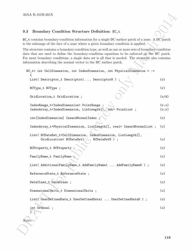
DRAFT

-For

publ

icre

view

only

Mar

ch20

14

AIAA R-101B-201X

9.3 Boundary Condition Structure Definition: BC_t

BC_t contains boundary-condition information for a single BC surface patch of a zone. A BC patchis the subrange of the face of a zone where a given boundary condition is applied.

The structure contains a boundary-condition type, as well as one or more sets of boundary-conditiondata that are used to define the boundary-condition equations to be enforced on the BC patch.For most boundary conditions, a single data set is all that is needed. The structure also containsinformation describing the normal vector to the BC surface patch.

BC_t< int CellDimension, int IndexDimension, int PhysicalDimension > :={List( Descriptor_t Descriptor1 ... DescriptorN ) ; (o)

BCType_t BCType ; (r)


IndexRange_t<IndexDimension> PointRange ; (r:o)IndexArray_t<IndexDimension, ListLength[], int> PointList ; (o:r)

int[IndexDimension] InwardNormalIndex ; (o)

IndexArray_t<PhysicalDimension, ListLength[], real> InwardNormalList ; (o)

List( BCDataSet_t<CellDimension, IndexDimension, ListLength[],GridLocation> BCDataSet1 ... BCDataSetN ) ; (o)

BCProperty_t BCProperty ; (o)








Notes

119

DRAFT

-For

publ

icre

view

only

Mar

ch20

14

AIAA R-101B-201X

1. Default names for the Descriptor_t, BCDataSet_t, and UserDefinedData_t lists are asshown; users may choose other legitimate names. Legitimate names must be unique withina given instance of BC_t and shall not include the names BCProperty, BCType, DataClass,DimensionalUnits, FamilyName, GridLocation, InwardNormalIndex, InwardNormalList,Ordinal, PointList, PointRange or ReferenceState.

2. GridLocation is optional; if absent its default value is Vertex. For other allowble values, seethe table below.

3. One of PointRange or PointList must be specified but not both. They must define a facesubrange of the zone.

4. InwardNormalIndex is only an option for structured grids. For unstructured grid boundaries,it should not be used. InwardNormalIndex may have only one nonzero element, whose signindicates the computational-coordinate direction of the BC patch normal; this normal pointsinto the interior of the zone.

5. InwardNormalList contains a list of vectors normal to the BC patch pointing into the interiorof the zone. It is a function of PhysicalDimension and ListLength[]. The vectors arelocated at the vertices of the BC patch when GridLocation is set to Vertex. Otherwise, theyare located at edge/face midpoints. The vectors are not required to have unit magnitude.

6. If PointRange and InwardNormalList are specified, an ordering convention is needed forindices on the BC patch. An ordering convention is also needed if a range is specified andlocal data is present in the BCDataSet_t substructures. FORTRAN multidimensional arrayordering is used.

BCType specifies the boundary-condition type, which gives general information on the boundary-condition equations to be enforced.

The BC patch may be specified by PointRange if it constitutes a logically rectangular region. Inall other cases, PointList should be used to list the vertices or cell edges/faces making up theBC patch. When GridLocation is set to Vertex, then PointList or PointRange refer to vertexindices, for both structured and unstructured grids. When GridLocation is set to EdgeCenter,then PointRange/List refer to edge elements. For 3–D grids, when GridLocation is set to Face-Center, IFaceCenter, etc., then PointRange/List refer to face elements. The interpretation ofPointRange/List is summarized in the table below:



Note: In the table, *FaceCenter stands for the possible types: FaceCenter, IFaceCenter, JFace-Center or KFaceCenter.

For structured grids, face centers are indexed using the minimum of the connecting vertex indices,as described in Section 3.2. For unstructured grids, edge and face elements are indexed using theirelement numbering as defined in the Elements_t data structures.

120

DRAFT

-For

publ

icre

view

only

Mar

ch20

14

AIAA R-101B-201X

The BC patch defined by PointRange/List is a surface region over which the particular set ofboundary conditions is applied. However, in the current standard there is no mechanism to specifywhether boundary conditions are enforced in the weak or strong form. If boundary conditions areimposed using collocation (i.e., strong form), there is also no requirement that they be imposedat the same locations used to define the BC patch (via PointRange/List). In the case when BCpatches are defined in terms of vertices (or edges in 3–D), then the bounding vertices will be locatedon multiple BC patches. If boundary conditions are imposed using collocation at vertices, then forthis case there is no mechanism to determine which BC patch takes precedence for any of thesebounding vertices.

Some boundary conditions require a normal direction to be specified in order to be properly imposed.For structured zones a computational-coordinate normal can be derived from the BC patch specifi-cation by examining redundant index components. Alternatively, for structured zones this informa-tion can be provided directly by InwardNormalIndex. From Note 4, this vector points into the zoneand can have only one non-zero element. For exterior faces of a zone in 3-D, InwardNormalIndexshould take the following values:

Face InwardNormalIndex Face InwardNormalIndex

i-min [+1, 0, 0] i-max [−1, 0, 0]j-min [0,+1, 0] j-max [0,−1, 0]k-min [0, 0,+1] k-max [0, 0,−1]

The physical-space normal vectors of the BC patch may be described by InwardNormalList; theseare located at vertices or cell faces, consistent with the BC patch specification. InwardNormalListis listed as an optional field because it is not always needed to enforce boundary conditions, andthe physical-space normals of a BC patch can usually be constructed from the grid. However, thereare some situations, such as grid-coordinate singularity lines, where InwardNormalList becomes arequired field, because it cannot be generated from other information.

The BC_t structure provides for a list of boundary-condition data sets, described in the next section.In general, the proper BCDataSet_t instance to impose on the BC patch is determined by the BCTypeassociation table (Table 4 on p. 133). The mechanics of determining the proper data set to imposeis described in Section 9.8.

For a few boundary conditions, such as a symmetry plane or polar singularity, the value of BCTypecompletely describes the equations to impose, and no instances of BCDataSet_t are needed. For“simple” boundary conditions, where a single set of Dirichlet and/or Neumann data is applied,a single BCDataSet_t will likely appear (although this is not a requirement). For “compound”boundary conditions, where the equations to impose are dependent on local flow conditions, severalinstances of BCDataSet_t will likely appear; the procedure for choosing the proper data set is morecomplex as described in Section 9.8.

A BCProperty_t data structure, described in Section 9.6, may be used to record special propertiesassociated with particular boundary condition patches, such as wall functions or bleed regions.

FamilyName identifies the family to which the boundary belongs. Family names link the meshboundaries to the CAD surfaces. (See Section 12.6.) Boundary conditions may also be defined

121

DRAFT-Forpublic

review

only


directly on families. In this case, the BCType must be FamilySpecified. If, under a BC_t structure,both FamilyName_t and BCType_t are present, and the BCType is not FamilySpecified, then theBCType that is specified takes precedence over any BCType that might be stored in a FamilyBC_tstructure under the specified Family_t.

Reference data applicable to the boundary conditions of a BC patch is contained in the Refer-enceState structure. DataClass defines the default for the class of data contained in the boundaryconditions. If the boundary conditions contain dimensional data, DimensionalUnits may be usedto describe the system of dimensional units employed. If present, these three entities take prece-dence over all corresponding entities at higher levels of the hierarchy. These precedence rules arefurther discussed in Section 6.4.


Ordinal is user-defined and has no restrictions on the values that it can contain. It is includedfor backward compatibility to assist implementation of the CGNS system into applications whoseI/O depends heavily on the numbering of BC patches. Since there are no restrictions on the valuescontained in Ordinal (or that Ordinal is even provided), there is no guarantee that the BC patchesfor a given zone in an existing CGNS database will have sequential values from 1 to N withoutholes or repetitions. Use of Ordinal is discouraged and is on a user-beware basis.



BC_t requires the structure function ListLength, which is used to specify the number of verticesor edge/face elements making up the BC patch. If PointRange is specified, then ListLengthis obtained from the number of points (inclusive) between the beginning and ending indices ofPointRange. If PointList is specified, then ListLength is the number of indices in the list ofpoints. In this situation, ListLength becomes a user input along with the indices of the listPointList. By “user” we mean the application code that is generating the CGNS database. IfElementRange or ElementList is specified, then ListLength is defined by the cell faces making upthe BC patch.

ListLength is also the number of elements in the list InwardNormalList. Note that syntacticallyPointList and InwardNormalList must have the same number of elements.

If neither PointRange or PointList is specified in a particular BCDataSet_t substructure, List-Length must be passed into it to determine the length of BC data arrays.

9.4 Boundary Condition Data Set Structure Definition: BCDataSet_t

BCDataSet_t contains Dirichlet and Neumann data for a single set of boundary-condition equations.Its intended use is for simple boundary-condition types, where the equations imposed do not dependon local flow conditions.

122

DRAFT

-For

publ

icre

view

only

Mar

ch20

14

AIAA R-101B-201X

BCDataSet_t< int CellDimension, int IndexDimension, int ListLengthParameter,GridLocation_t GridLocationParameter > :=


BCTypeSimple_t BCTypeSimple ; (r)

BCData_t<ListLengthBCData[]> DirichletData ; (o)BCData_t<ListLengthBCData[]> NeumannData ; (o)


IndexRange_t<IndexDimension> PointRange ; (o)IndexArray_t<IndexDimension, ListLength, int> PointList ; (o)





Notes

1. Default names for the Descriptor_t and UserDefinedData_t lists are as shown; users maychoose other legitimate names. Legitimate names must be unique within a given instance ofBCDataSet_t and shall not include the names BCTypeSimple, DataClass, DimensionalUnits,DirichletData, GridLocation, NeumannData, PointList, PointRange, or ReferenceState.

2. BCTypeSimple is the only required field. All other fields are optional and the Descriptor_tlist may be empty.

3. GridLocation is optional; if absent its default value is GridLocationParameter. For 2–Dgrids (CellDimension = 2), GridLocation may take the values of Vertex or EdgeCenter. For3–D grids (CellDimension = 3), GridLocation may take the values of Vertex, EdgeCenter,FaceCenter, IFaceCenter, JFaceCenter or KFaceCenter.

4. PointRange and PointList are both optional; only one of them may be specified. They mustdefine a face subrange of the zone.

BCDataSet_t requires the structure parameters CellDimension, IndexDimension, ListLengthPa-rameter and GridLocationParameter. These are all used to control the grid location and lengthof data arrays in the Dirichlet and Neumann substructures. They are inputs for the structurefunctions ListLength[] and ListLengthBCData[] defined below.

BCTypeSimple specifies the boundary-condition type, which gives general information on the bound-ary-condition equations to be enforced. BCTypeSimple_t is defined in Section 9.7 along with the

123

DRAFT

-For

publ

icre

view

only

Mar

ch20

14

AIAA R-101B-201X

meanings of all the BCTypeSimple values. BCTypeSimple is also used for matching boundarycondition data sets as discussed in Section 9.8.

Boundary-condition data is separated by equation type into Dirichlet and Neumann conditions.Dirichlet boundary conditions impose the value of the given variables, whereas Neumann boundaryconditions impose the normal derivative of the given variables. The mechanics of specifying Dirichletand Neumann data for boundary conditions is covered in Section 9.9.

The substructures DirichletData and NeumannData contain boundary-condition data that maybe constant over the BC patch or defined locally at each vertex or edge/face of the patch. Locallydefined data can be specified in one of two ways. If GridLocation, PointRange and PointList areall absent, then the data is defined consistent with the BC patch specification of the parent BC_tstructure. In this case, the location of the locally defined data is given by GridLocationParameterand the length of the data arrays are given by ListLengthParameter. If GridLocation and oneof PointRange or PointList is present, then the same rules provided in Section 9.3 apply. In thiscase, the length of the data arrays is given by ListLength[].

Reference quantities applicable to the set of boundary-condition data are contained in the Refer-enceState structure. DataClass defines the default for the class of data contained in the boundary-condition data. If the boundary conditions contain dimensional data, DimensionalUnits may beused to describe the system of dimensional units employed. If present, these three entities takeprecedence over all corresponding entities at higher levels of the hierarchy. These precedence rulesare further discussed in Section 6.4.




BCDataSet_t requires the structure function ListLength, which is used to specify the length oflocally defined Dirichlet and Neumann data arrays when the grid location of these quantities differsfrom that of the BC patch definition. The definition of ListLength is identical to that provided inBC_t (Section 9.3).

FUNCTION ListLengthBCData[]:

return value: intdependencies: ListLengthParameter, PointRange, PointList

BCDataSet_t also requires the structure function ListLengthBCData. If PointRange or PointListis present, then ListLengthBCData takes the value of ListLength. If both are absent, then it takesthe value ListLengthParameter.

124

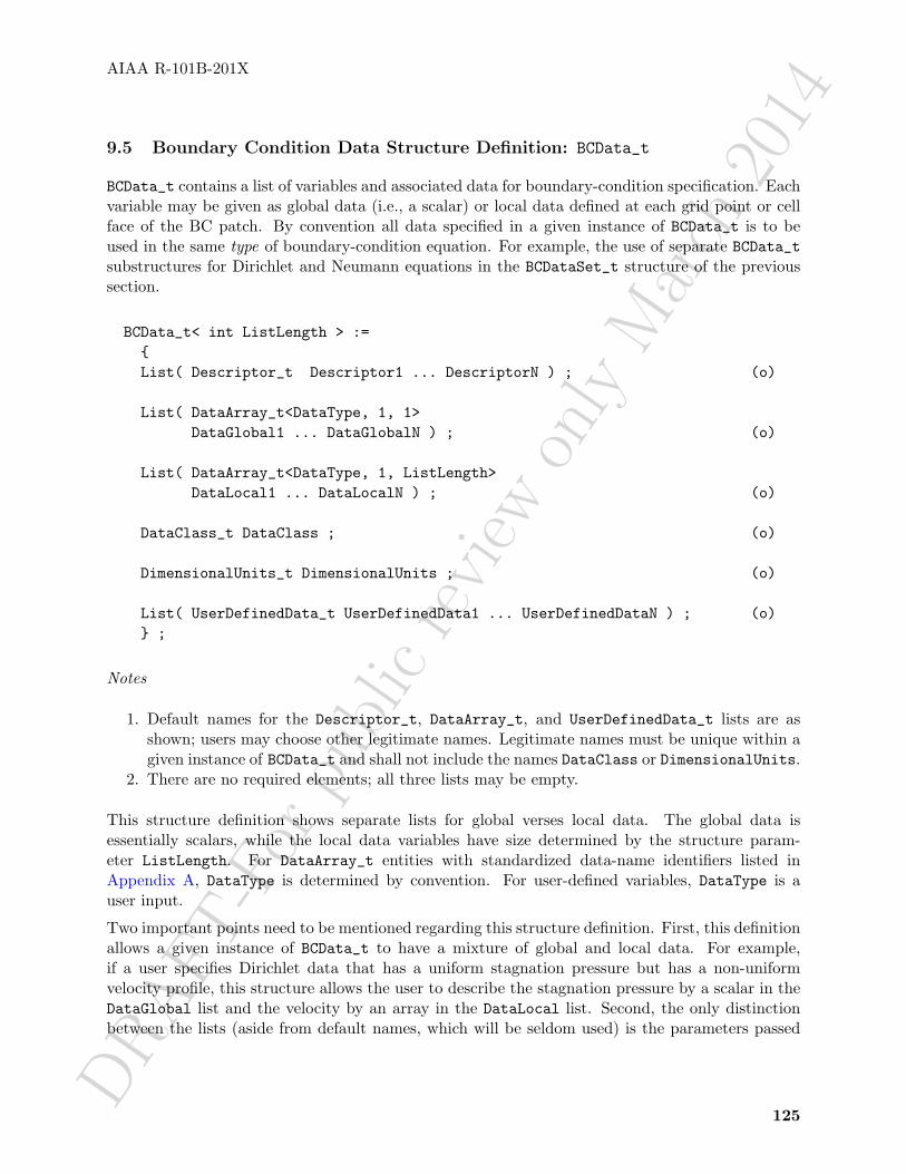
DRAFT

-For

publ

icre

view

only

Mar

ch20

14

AIAA R-101B-201X

9.5 Boundary Condition Data Structure Definition: BCData_t

BCData_t contains a list of variables and associated data for boundary-condition specification. Eachvariable may be given as global data (i.e., a scalar) or local data defined at each grid point or cellface of the BC patch. By convention all data specified in a given instance of BCData_t is to beused in the same type of boundary-condition equation. For example, the use of separate BCData_tsubstructures for Dirichlet and Neumann equations in the BCDataSet_t structure of the previoussection.

BCData_t< int ListLength > :={List( Descriptor_t Descriptor1 ... DescriptorN ) ; (o)

List( DataArray_t<DataType, 1, 1>DataGlobal1 ... DataGlobalN ) ; (o)

List( DataArray_t<DataType, 1, ListLength>DataLocal1 ... DataLocalN ) ; (o)




Notes

1. Default names for the Descriptor_t, DataArray_t, and UserDefinedData_t lists are asshown; users may choose other legitimate names. Legitimate names must be unique within agiven instance of BCData_t and shall not include the names DataClass or DimensionalUnits.

2. There are no required elements; all three lists may be empty.

This structure definition shows separate lists for global verses local data. The global data isessentially scalars, while the local data variables have size determined by the structure param-eter ListLength. For DataArray_t entities with standardized data-name identifiers listed inAppendix A, DataType is determined by convention. For user-defined variables, DataType is auser input.

Two important points need to be mentioned regarding this structure definition. First, this definitionallows a given instance of BCData_t to have a mixture of global and local data. For example,if a user specifies Dirichlet data that has a uniform stagnation pressure but has a non-uniformvelocity profile, this structure allows the user to describe the stagnation pressure by a scalar in theDataGlobal list and the velocity by an array in the DataLocal list. Second, the only distinctionbetween the lists (aside from default names, which will be seldom used) is the parameters passed

125

DRAFT

-For

publ

icre

view

only

Mar

ch20

14

AIAA R-101B-201X

into the DataArray_t structure. Therefore, in actual implementation of this BCData_t structure itmay not be possible to distinguish between members of the global and local lists without queryinginside the DataArray_t substructures. Straightforward mapping onto the ADF or HDF databasewill not provide any distinctions between the members of the two lists. This hopefully will notcause any problems.

DataClass defines the default for the class of data contained in the boundary-condition data. If theboundary-condition data is dimensional, DimensionalUnits may be used to describe the system ofdimensional units employed. If present, these two entities take precedence over all correspondingentities at higher levels of the hierarchy. These precedence rules are further discussed in Section 6.4.


9.6 Boundary Condition Property Structure Definition: BCProperty_t

BCProperty_t allows the recording of special properties associated with particular boundary con-dition patches. At the current time, only two properties (WallFunction_t and Area_t) are in-cluded, but extensions involving boundary conditions may be implemented as additional nodesunder BCProperty_t in the future.

BCProperty_t :={List( Descriptor_t Descriptor1 ... DescriptorN ) ; (o)

WallFunction_t WallFunction ; (o)

Area_t Area ; (o)


Notes

1. Default names for the Descriptor_t, DataArray_t, and UserDefinedData_t lists are asshown; users may choose other legitimate names. Legitimate names must be unique within agiven instance of BCProperty_t and shall not include the names WallFunction or Area.

The WallFunction_t and Area_t data structures may be used to record properties associated withthe use of wall functions, or area-related boundary conditions such as bleed, respectively.


126

DRAFT

-For

publ

icre

view

only

Mar

ch20

14

AIAA R-101B-201X

9.6.1 Wall Function Structure Definition: WallFunction_t

The WallFunction_t data structure allows data associated with the use of wall function boundaryconditions to be recorded.

WallFunction_t :={List( Descriptor_t Descriptor1 ... DescriptorN ) ; (o)

WallFunctionType_t WallFunctionType ; (r)


Notes

1. Default names for the Descriptor_t and UserDefinedData_t lists are as shown; users maychoose other legitimate names. Legitimate names must be unique within a given instance ofWallFunction_t and shall not include the name WallFunctionType.

WallFunctionType_t is a required enumeration data structure that is used to define the type ofwall functions being used.

WallFunctionType_t := Enumeration(WallFunctionTypeNull,WallFunctionTypeUserDefined,Generic ) ;

Because there is such a wide array of methods for employing wall functions (few of which are well-documented), the type Generic is used to simply indicate that a wall function is employed, withoutspecifying details.

9.6.2 Area Structure Definition: Area_t

The Area_t data structure allows data associated with area-related boundary conditions such asbleed to be recorded.

Area_t :={List( Descriptor_t Descriptor1 ... DescriptorN ) ; (o)

AreaType_t AreaType ; (r)DataArray_t<real, 1, 1> SurfaceArea ; (r)DataArray_t<real, 1, 32> RegionName ; (r)

127

DRAFT-Forpublic

review

only



Notes

1. Default names for the Descriptor_t and UserDefinedData_t lists are as shown; users maychoose other legitimate names. Legitimate names must be unique within a given instance ofArea_t and shall not include the names AreaType, RegionName, or SurfaceArea.

AreaType_t is a required enumeration data structure that is used to define the type of area beingdefined.

AreaType_t := Enumeration(AreaTypeNull,AreaTypeUserDefined,BleedArea,CaptureArea ) ;

If AreaType is set to BleedArea, the value of SurfaceArea is the size of the current bleed surface.Note that bleed is commonly used with wall boundary conditions. The bleed area is the surfacearea of the boundary condition patch.

If AreaType is set to CaptureArea, then SurfaceArea represents the size of the current capturesurface. For inlet flows, for example, the capture area is the area of a fictitious surface in frontof the inlet in which mass is pulled into the inlet. This is used to calculate the mass flow for theboundary condition patch based on the formula:

mass flow = MFR ρ∞U∞Acap

where MFR is the desired mass flow ratio and Acap is the capture area. Another interpretation isthe far-upstream cross-sectional area of the stream tube that feeds the inlet. Note that the capturearea is usually defined with an outflow boundary condition, which is commonly used at an engineface.

The RegionName is character identifier, and is needed so that a specific region can span multiplesurfaces over multiple zones.

9.7 Boundary Condition Type Structure Definition: BCType_t

BCType_t is an enumeration type that identifies the boundary-condition equations to be enforcedat a given boundary location.

BCType_t := Enumeration(BCTypeNull, BCTypeUserDefined, BCAxisymmetricWedge, BCDegenerateLine.BCDegeneratePoint, BCDirichlet, BCExtrapolate, BCFarfield, BCGeneral,

128

DRAFT

-For

publ

icre

view

only

Mar

ch20

14

AIAA R-101B-201X

BCInflow, BCInflowSubsonic, BCInflowSupersonic, BCNeumann,BCOutflow, BCOutflowSubsonic, BCOutflowSupersonic, BCSymmetryPlane,BCSymmetryPolar, BCTunnelInflow, BCTunnelOutflow, BCWall,BCWallInviscid, BCWallViscous, BCWallViscousHeatFlux,BCWallViscousIsothermal, FamilySpecified ) ;

The boundary-condition type is further defined as simple, BCTypeSimple_t, or compound, BCType-Compound_t, which are subsets of the enumeration type BCType_t.

BCTypeSimple_t := Enumeration(BCTypeNull, BCTypeUserDefined, BCAxisymmetricWedge, BCDegenerateLine.BCDegeneratePoint, BCDirichlet, BCExtrapolate, BCGeneral,BCInflowSubsonic, BCInflowSupersonic, BCNeumann,BCOutflowSubsonic, BCOutflowSupersonic, BCSymmetryPlane,BCSymmetryPolar, BCTunnelInflow, BCTunnelOutflow, BCWall,BCWallInviscid, BCWallViscous, BCWallViscousHeatFlux,BCWallViscousIsothermal, FamilySpecified ) ;

BCTypeCompound_t := Enumeration(BCTypeNull, BCTypeUserDefined, BCInflow, BCOutflow,BCFarfield ) ;

The members of BCTypeSimple_t completely identify the equations to impose, while those of BC-TypeCompound_t give a general description of the class of boundary-condition equations to impose.The specific boundary-condition equations to enforce for each value of BCType_t are listed in Table 2and Table 3.

The subdivision of BCType_t is based on function. For simple boundary conditions, the equationsand data imposed are fixed; whereas, for compound boundary conditions different sets of equationsare imposed depending on local flow conditions at the boundary. This distinction requires additionalrules for dealing with simple and compound boundary-condition types. These rules are discussedin Section 9.8.

For the inflow/outflow boundary-condition descriptions, 3-D inviscid compressible flow is assumed;the 2-D equivalent should be obvious. These same boundary conditions are typically used forviscous cases also. This “3-D Euler” assumption will be noted wherever used.

In the following tables, Q is the solution vector, ~q is the velocity vector whose magnitude is q, theunit normal to the boundary is n, and ∂()/∂n = n·∇ is differentiation normal to the boundary.

Table 2: Simple Boundary Condition Types

BCType_t orBCTypeSimple_t Identifier

Boundary Condition Description

BCGeneral Arbitrary conditions on Q or ∂Q/∂n

Continued on next page

129

DRAFT

-For

publ

icre

view

only

Mar

ch20

14

AIAA R-101B-201X

Table 2: Simple Boundary Condition Types (Continued)



BCDirichlet Dirichlet condition on Q vector

BCNeumann Neumann condition on ∂Q/∂n

BCExtrapolate Extrapolate Q from interior

BCWallInviscid Inviscid (slip) wall• normal velocity specified (default: ~q · n = 0)

BCWallViscousHeatFlux Viscous no-slip wall with heat flux• velocity Dirichlet (default: q = 0)• temperature Neumann (default: adiabatic, ∂T/∂n = 0)

BCWallViscousIsothermal Viscous no-slip, isothermal wall• velocity Dirichlet (default: q = 0)• temperature Dirichlet

BCWallViscous Viscous no-slip wall; special cases areBCWallViscousHeatFlux and BCWallViscousIsothermal• velocity Dirichlet (default: q = 0)• Dirichlet or Neumann on temperature

BCWall General wall condition; special cases are BCWallInviscid,BCWallViscous, BCWallViscousHeatFlux andBCWallViscousIsothermal

BCInflowSubsonic Inflow with subsonic normal velocity• specify 4; extrapolate 1 (3-D Euler)

BCInflowSupersonic Inflow with supersonic normal velocity• specify 5; extrapolate 0 (3-D Euler)

Same as BCDirichlet

BCOutflowSubsonic Outflow with subsonic normal velocity• specify 1; extrapolate 4 (3-D Euler)

BCOutflowSupersonic Outflow with supersonic normal velocity• specify 0; extrapolate 5 (3-D Euler)

Same as BCExtrapolate

BCTunnelInflow Tunnel inlet (subsonic normal velocity)• specify cross-flow velocity, stagnation enthalpy, entropy• extrapolate 1 (3-D Euler)


130

DRAFT

-For

publ

icre

view

only

Mar

ch20

14

AIAA R-101B-201X

Table 2: Simple Boundary Condition Types (Continued)



BCTunnelOutflow Tunnel exit (subsonic normal velocity)• specify static pressure• extrapolate 4 (3-D Euler)

BCDegenerateLine Face degenerated to a line

CCCCCC��HHHHHHLLLL

BCDegeneratePoint Face degenerated to a point

CCCCCCXXXXXXXXXLLLL

BCSymmetryPlane Symmetry plane; face should be coplanar• density, pressure: ∂()/∂n = 0• tangential velocity: ∂(~q×n)/∂n = 0• normal velocity: ~q · n = 0

BCSymmetryPolar Polar-coordinate singularity line; special case ofBCDegenerateLine where degenerate face is a straight lineand flowfield has polar symmetry; s is singularity linetangential unit vector• normal velocity: ~q×s = 0• all others: ∂()/∂n = 0, n normal to s

BCAxisymmetricWedge Axisymmetric wedge; special case of BCDegenerateLinewhere degenerate face is a straight line

FamilySpecified A boundary condition type is being specified for the family towhich the current boundary belongs. A FamilyName_tspecification must exist under BC_t, corresponding to aFamily_t structure under CGNSBase_t. Under the Family_tstructure there must be a FamilyBC_t structure specifying avalid BCType (other than FamilySpecified!). If any of theseare absent, the boundary condition type is undefined.

131

DRAFT

-For

publ

icre

view

only

Mar

ch20

14

AIAA R-101B-201X

Table 3: Compound Boundary Condition Types

BCType_t orBCTypeCompound_t Identifier


BCInflow Inflow, arbitrary normal Mach; test on normal Mach, thenperform one of: BCInflowSubsonic, BCInflowSupersonic

BCOutflow Outflow, arbitrary normal Mach; test on normal Mach,then perform one of: BCOutflowSubsonic,BCOutflowSupersonic

BCFarfield Farfield inflow/outflow, arbitrary normal Mach; test onnormal velocity and normal Mach, then perform one of:BCInflowSubsonic, BCInflowSupersonic,BCOutflowSubsonic, BCOutflowSupersonic

9.8 Matching Boundary Condition Data Sets

The BC_t structure allows for a arbitrary list of boundary-condition data sets, described by theBCDataSet_t structure. For simple boundary conditions, a single data set must be chosen froma list that may contain more than one element. Likewise, for a compound boundary condition, alimited number of data sets must be chosen and applied appropriately. The mechanism for theproper choice of data sets is controlled by the BCType field of the BC_t structure, the BCTypeSimplefield of the BCDataSet_t structure, and the boundary-condition type association table (Table 4).In the following discussion, we will use the “/” notation for fields or elements of a structure type.

BC_t is used for both simple and compound boundary conditions; hence, the field BC_t/BCTypeis of type BCType_t. Conversely, the substructure BCDataSet_t is intended to enforce a singleset of boundary-condition equations independent of local flow conditions (i.e., it is appropriateonly for simple boundary conditions). This is why the field BCDataSet_t/BCTypeSimple is of typeBCTypeSimple_t and not BCType_t. The appropriate choice of data sets is determined by matchingthe field BC_t/BCType with the field BCDataSet_t/BCTypeSimple as specified in Table 4.

For simple boundary conditions, a single match from the list of BCDataSet_t instances is required.For all BCTypeSimple_t identifiers, except BCInflowSupersonic and BCOutflowSupersonic, anexact match is necessary. BCInflowSupersonic will match itself or BCDirichlet; BCOutflowSu-personic will match itself or BCExtrapolate.

For compound boundary conditions, the association table specifies which simple boundary-conditiontypes are appropriate. Since compound boundary conditions enforce different boundary-conditionequation sets depending on local flow conditions, several instances of BCDataSet_t will be matchedfor each BCTypeCompound_t identifier. The accompanying rule determines which of the matchingdata sets to apply at a given location on the BC patch.

This provides a general procedure applicable to both BCTypeSimple_t and BCTypeCompound_t situ-ations. For a given BC_t/BCType use those instances of BCDataSet_t whose field BCDataSet_t/BC-TypeSimple matches according to Table 4. Apply the matching data set or sets as prescribed bythe appropriate usage rule.

132

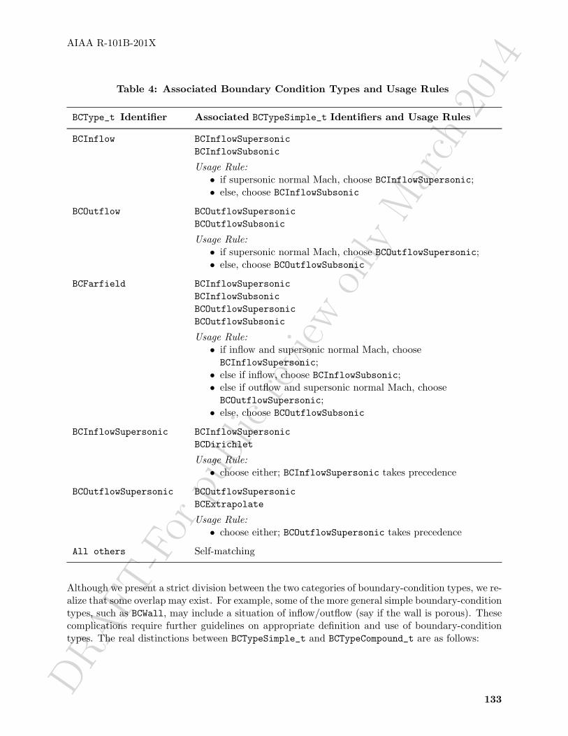
DRAFT

-For

publ

icre

view

only

Mar

ch20

14

AIAA R-101B-201X

Table 4: Associated Boundary Condition Types and Usage Rules

BCType_t Identifier Associated BCTypeSimple_t Identifiers and Usage Rules

BCInflow BCInflowSupersonicBCInflowSubsonic

Usage Rule:• if supersonic normal Mach, choose BCInflowSupersonic;• else, choose BCInflowSubsonic

BCOutflow BCOutflowSupersonicBCOutflowSubsonic

Usage Rule:• if supersonic normal Mach, choose BCOutflowSupersonic;• else, choose BCOutflowSubsonic

BCFarfield BCInflowSupersonicBCInflowSubsonicBCOutflowSupersonicBCOutflowSubsonic

Usage Rule:• if inflow and supersonic normal Mach, chooseBCInflowSupersonic;• else if inflow, choose BCInflowSubsonic;• else if outflow and supersonic normal Mach, chooseBCOutflowSupersonic;• else, choose BCOutflowSubsonic

BCInflowSupersonic BCInflowSupersonicBCDirichlet

Usage Rule:• choose either; BCInflowSupersonic takes precedence

BCOutflowSupersonic BCOutflowSupersonicBCExtrapolate

Usage Rule:• choose either; BCOutflowSupersonic takes precedence

All others Self-matching

Although we present a strict division between the two categories of boundary-condition types, we re-alize that some overlap may exist. For example, some of the more general simple boundary-conditiontypes, such as BCWall, may include a situation of inflow/outflow (say if the wall is porous). Thesecomplications require further guidelines on appropriate definition and use of boundary-conditiontypes. The real distinctions between BCTypeSimple_t and BCTypeCompound_t are as follows:

133

DRAFT

-For

publ

icre

view

only

Mar

ch20

14

AIAA R-101B-201X

• BCTypeSimple_t identifiers always match themselves; BCTypeCompound_t identifiers nevermatch themselves.

• BCTypeSimple_t identifiers always produce a single match; BCTypeCompound_t will producemultiple matches.

• The usage rule for BCTypeSimple_t identifiers is always trivial—apply the single matchingdata set regardless of local flow conditions.

Therefore, any boundary condition that involves application of different data sets depending onlocal flow conditions should be classified BCTypeCompound_t. If a type that we have classifiedBCTypeSimple_t is used as a compound type (BCWall for a porous wall is an example), then itshould somehow be reclassified. One option is to define a new BCTypeCompound_t identifier andprovide associated BCTypeSimple_t types and a usage rule. Another option may be to allow someidentifiers to be both BCTypeSimple_t and BCTypeCompound_t and let their appropriate use bebased on context. This is still undetermined.

9.9 Boundary Condition Specification Data

For a given simple boundary condition (i.e., one that is not dependent on local flow conditions),the database provides a set of boundary-condition equations to be enforced through the structuredefinitions for BCDataSet_t and BCData_t (Section 9.4 and Section 9.5). Apart from the boundary-condition type, the precise equations to be enforced are described by boundary-condition solutiondata. These specified solution data are arranged by “equation type”:

Dirichlet: Q = (Q)specified

Neumann: ∂Q/∂n = (∂Q/∂n)specified

The DirichletData and NeumannData entities of BCData_t list both the solution variables involvedin the equations (through the data-name identifier conventions of Appendix A) and the specifiedsolution data.

Two issues need to be addressed for specifying Dirichlet or Neumann boundary-condition data.The first is whether the data is global or local:

Global BC data: Data applied globally to the BC patch; for example, specifying a uniformtotal pressure at an inflow boundary

Local BC data: Data applied locally at each vertex or cell face of the BC patch; an exampleof this is varying total pressure specified at each grid point at an inflowboundary

The second issue is describing the actual solution quantities that are to be specified. Both of theseissues are addressed by use of the DataArray_t structure.

134

DRAFT

-For

publ

icre

view

only

Mar

ch20

14

AIAA R-101B-201X

For some types of boundary conditions, many different combinations of solution quantities couldbe specified. For example, BCInflowSubsonic requires 4 solution quantities to be specified in 3-D,but what those 4 quantities are varies with applications (e.g., internal verses external flows) andcodes. We propose the convention that the actual data being specified for any BCType is given bythe list of DataArray_t entities included in DirichletData and NeumannData structures (actuallyby the identifier attached to each instance of DataArray_t). This frees us from having to definemany versions of a given BCType (e.g., BCInflowSubsonic1, BCInflowSubsonic2, etc.), where eachhas a precisely defined set of Dirichlet data. We are left with the easier task of defining how manyDirichlet or Neumann quantities must be provided for each BCType.

An example of using DataArray_t-identifier conventions to describe BC specification data is thefollowing: subsonic inflow with uniform stagnation pressure, mass flow and cross-flow angle speci-fied; the Dirichlet data are stagnation pressure = 2.56, mass flow = 1.34, and cross-flow angle hasa y-component of 0.043 and a z-component of 0.02 (ignore dimensional-units or normalization forthe present). The specified solution variables and associated data are described as shown:

BCData_t<ListLength=?> DirichletData ={{DataArray_t<real, 1, 1> PressureStagnation = {{ Data(real, 1, 1) = 2.56 }} ;DataArray_t<real, 1, 1> MassFlow = {{ Data(real, 1, 1) = 1.34 }} ;DataArray_t<real, 1, 1> VelocityAngleY = {{ Data(real, 1, 1) = 0.043 }} ;DataArray_t<real, 1, 1> VelocityAngleZ = {{ Data(real, 1, 1) = 0.02 }} ;}} ;

Basically, this states that DirichletData contains four instances of DataArray_t with identifiersor names PressureStagnation, MassFlow, VelocityAngleY and VelocityAngleZ. Each DataAr-ray_t structure entity contains a single floating-point value; these are the Dirichlet data for theBC. Note that Data(real, 1, 1) means a single floating-point value.

The global verses local data issue can be easily handled by storing either a scalar, as shown above,for the global BC data case; or storing an array for the local BC data case. Storing an array oflocal BC data allows the capability for specifying non-constant solution profiles, such as “analytic”boundary-layer profiles or profiles derived from experimental data. For the above example, if thestagnation pressure is instead specified at every vertex of the boundary-condition patch the followingresults:

BCData_t<ListLength=99> DirichletData ={{DataArray_t<real, 1, 99> PressureStagnation ={{ Data(real, 1, 99) = (PTOT(n), n=1,99) }} ;

DataArray_t<real, 1, 1> MassFlow = {{ Data(real, 1, 1) = 1.34 }} ;DataArray_t<real, 1, 1> VelocityAngleY = {{ Data(real, 1, 1) = 0.043 }} ;DataArray_t<real, 1, 1> VelocityAngleZ = {{ Data(real, 1, 1) = 0.02 }} ;}} ;

where, say, the boundary face is logically rectangular and contains 11×9 vertices and the stagnationpressure at the vertices is given by the array PTOT().

135

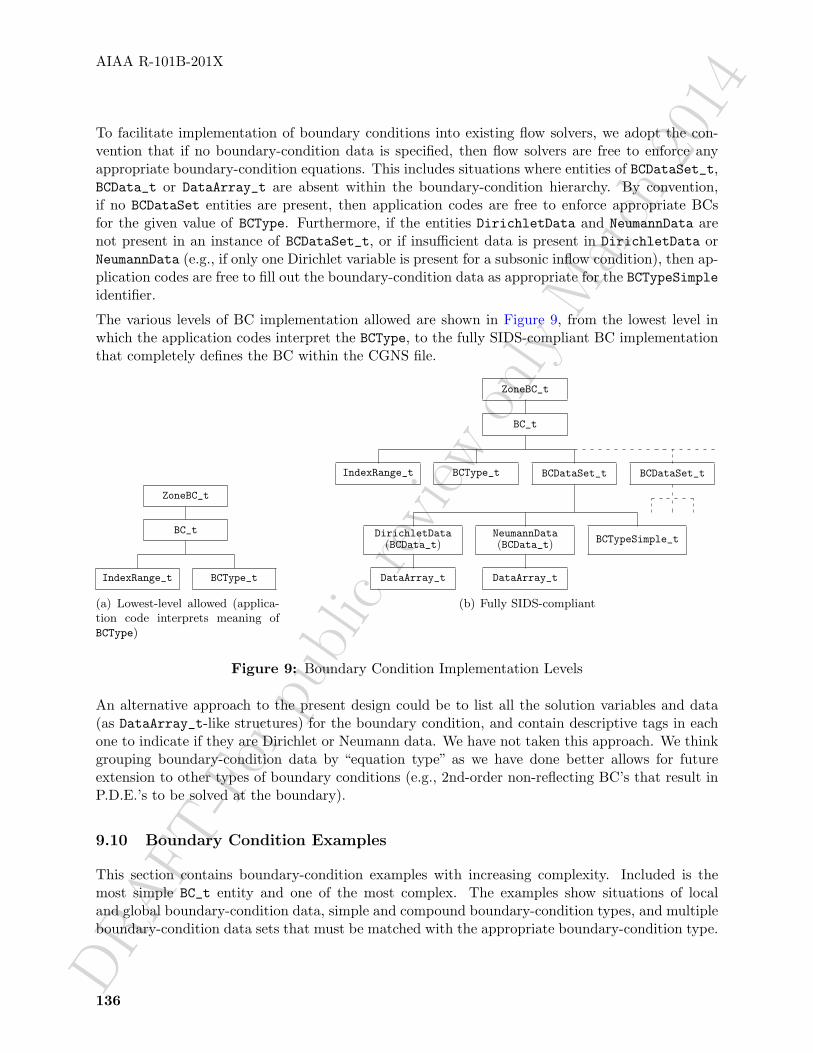
DRAFT

-For

publ

icre

view

only

Mar

ch20

14

AIAA R-101B-201X

To facilitate implementation of boundary conditions into existing flow solvers, we adopt the con-vention that if no boundary-condition data is specified, then flow solvers are free to enforce anyappropriate boundary-condition equations. This includes situations where entities of BCDataSet_t,BCData_t or DataArray_t are absent within the boundary-condition hierarchy. By convention,if no BCDataSet entities are present, then application codes are free to enforce appropriate BCsfor the given value of BCType. Furthermore, if the entities DirichletData and NeumannData arenot present in an instance of BCDataSet_t, or if insufficient data is present in DirichletData orNeumannData (e.g., if only one Dirichlet variable is present for a subsonic inflow condition), then ap-plication codes are free to fill out the boundary-condition data as appropriate for the BCTypeSimpleidentifier.

The various levels of BC implementation allowed are shown in Figure 9, from the lowest level inwhich the application codes interpret the BCType, to the fully SIDS-compliant BC implementationthat completely defines the BC within the CGNS file.

ZoneBC_t

BC_t

IndexRange_t BCType_t

(a) Lowest-level allowed (applica-tion code interprets meaning ofBCType)

ZoneBC_t

BC_t

IndexRange_t BCType_t BCDataSet_t BCDataSet_t

DirichletData(BCData_t)

NeumannData(BCData_t) BCTypeSimple_t

DataArray_tDataArray_t

(b) Fully SIDS-compliant

Figure 9: Boundary Condition Implementation Levels

An alternative approach to the present design could be to list all the solution variables and data(as DataArray_t-like structures) for the boundary condition, and contain descriptive tags in eachone to indicate if they are Dirichlet or Neumann data. We have not taken this approach. We thinkgrouping boundary-condition data by “equation type” as we have done better allows for futureextension to other types of boundary conditions (e.g., 2nd-order non-reflecting BC’s that result inP.D.E.’s to be solved at the boundary).

9.10 Boundary Condition Examples

This section contains boundary-condition examples with increasing complexity. Included is themost simple BC_t entity and one of the most complex. The examples show situations of localand global boundary-condition data, simple and compound boundary-condition types, and multipleboundary-condition data sets that must be matched with the appropriate boundary-condition type.

136

DRAFT-Forpublic

review

only


Example 9-A: Symmetry Plane

Symmetry plane for a patch on the i-min face of a 3-D structured zone.

! CellDimension = 3, IndexDimension = 3BC_t<3,3,3> BC1 ={{BCType_t BCType = BCSymmetryPlane ;

IndexRange_t<3> PointRange ={{int[3] Begin = [1,1,1 ] ;int[3] End = [1,9,17] ;}} ;

}} ;

Since the boundary-condition equations to be enforced are completely defined by the boundary-condition type BCSymmetryPlane, no other information needs to be provided, except for the extentof the BC patch. The BC patch is specified by PointRange with a beginning index of (1,1,1) andan ending index of (1,9,17). By default, these refer to vertices.

Example 9-B: Viscous Solid Wall I

A viscous solid wall for a 3-D structured zone, where a Dirichlet condition is enforced for temper-ature; the wall temperature for the entire wall is specified to be 273 K. The BC patch is on thej-min face and is bounded by the indices (1,1,1) and (33,1,9).

! CellDimension = 3, IndexDimension = 3BC_t<3,3,3> BC2 ={{BCType_t BCType = BCWallViscousIsothermal ;

IndexRange_t<3> PointRange ={{int[3] Begin = [1 ,1,1] ;int[3] End = [33,1,9] ;}} ;

! ListLength = 33*9 = 297BCDataSet_t<297> BCDataSet1 ={{BCTypeSimple_t BCTypeSimple = BCWallViscousIsothermal ;

! Data array length = ListLength = 297BCData_t<297> DirichletData ={{DataArray_t<real, 1, 1> Temperature =

137

DRAFT

-For

publ

icre

view

only

Mar

ch20

14

AIAA R-101B-201X

{{Data(real, 1, 1) = 273. ;


DimensionalUnits_t DimensionalUnits ={{MassUnits = MassUnitsNull ;LengthUnits = LengthUnitsNull ;TimeUnits = TimeUnitsNull ;TemperatureUnits = Kelvin ;AngleUnits = AngleUnitsNull ;}} ;

}} ;}} ;

}} ;}} ;

This is an example of a simple boundary-condition type, BCWallViscousIsothermal. By defaultthere is a zero Dirichlet condition on the velocity, and BCDataSet1 states there is a Dirichlet condi-tion on temperature with a global value of 273 K. The data set contains a single BCData_t entity,called DirichletData, meaning a (possibly empty) collection of Dirichlet conditions should be en-forced. Within DirichletData, there is a single DataArray_t entity; this narrows the specificationto a single Dirichlet condition. This lone entity has the identifier Temperature, which by conventionsdefined in Appendix A is the identifier for static temperature. The data contained in Temperatureis a floating-point scalar with a value of 273. The qualifiers DataClass and DimensionalUnitsspecify that the temperature is dimensional with units of Kelvin.

Since BCWallViscousIsothermal is a simple boundary-condition type, the appropriate data setcontains a BCTypeSimple entity whose value is BCWallViscousIsothermal. For this example, onlya single data set is provided, and this data set has the correct boundary-condition type. This is anexample of a trivial data-set match.

Apart from velocity and temperature, additional “numerical” boundary conditions are typicallyrequired by Navier-Stokes flow solvers, but none are given here; therefore, a code is free to implementother additional boundary conditions as desired.

Although the boundary-condition data is global, we include in this example structure parametersthat are the lengths of potential local-data arrays. Comments are added to the example with the“!” notation to document the structure parameters. The BC_t structure function ListLength isevaluated based on PointRange. Since GridLocation is not specified in BC2, any local data is atvertices by default. The entity Temperature contains global data, so the value of ListLength isunused in DirichletData.

This example raises the question of whether unused structure parameters are required in structureentities. The answer is no. We included them here for completeness. The purpose of structureparameters is to mimic the need to define elements of a entity based on information containedelsewhere (at a higher level) in the CGNS database. When this need is not present in a given

138

DRAFT-Forpublic

review

only


instance of a structure entity, the structure parameters are superfluous. In some of the followingexamples, structure parameters that are superfluous or otherwise not needed are denoted by “?”.

Example 9-C: Subsonic Inflow

Subsonic inflow for a 2-D structured zone: The BC patch is on the i-min face and includes j ∈ [2, 7].As prescribed by the boundary-condition type, three quantities must be specified. Uniform entropyand stagnation enthalpy are specified with values of 0.94 and 2.85, respectively. A velocity profileis specified at face midpoints, given by the array v_inflow(j). No dimensional or nondimensionalinformation is provided.

! CellDimension = 2, IndexDimension = 2BC_t<2,2,?> BC3 ={{BCType_t BCType = BCInflowSubsonic ;

GridLocation_t GridLocation = FaceCenter ;

IndexRange_t<2> PointRange ={{int[2] Begin = [1,2] ;int[2] End = [1,6] ;}} ;

! ListLength = 5BCDataSet_t<5> BCDataSet1 ={{BCTypeSimple_t BCTypeSimple = BCInflowSubsonic ;

! Data array length = ListLength = 5BCData_t<5> DirichletData ={{DataArray_t<real, 1, 1> EntropyApprox ={{Data(real, 1, 1) = 0.94 ;}} ;

DataArray_t<real, 1, 1> EnthalpyStagnation ={{Data(real, 1, 1) = 2.85 ;}} ;

DataArray_t<real, 1, 5> VelocityY ={{Data(real, 1, 5) = (v_inflow(j), j=3,7) ;}} ;

139

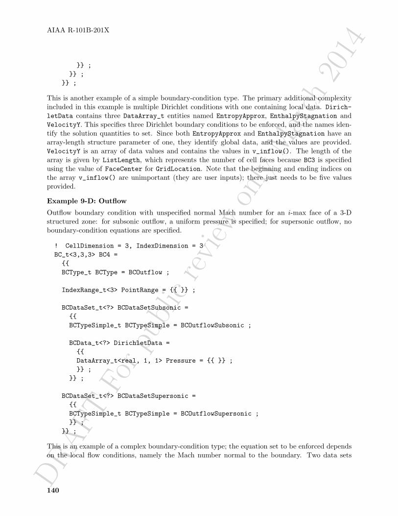
DRAFT

-For

publ

icre

view

only

Mar

ch20

14

AIAA R-101B-201X

}} ;}} ;

}} ;

This is another example of a simple boundary-condition type. The primary additional complexityincluded in this example is multiple Dirichlet conditions with one containing local data. Dirich-letData contains three DataArray_t entities named EntropyApprox, EnthalpyStagnation andVelocityY. This specifies three Dirichlet boundary conditions to be enforced, and the names iden-tify the solution quantities to set. Since both EntropyApprox and EnthalpyStagnation have anarray-length structure parameter of one, they identify global data, and the values are provided.VelocityY is an array of data values and contains the values in v_inflow(). The length of thearray is given by ListLength, which represents the number of cell faces because BC3 is specifiedusing the value of FaceCenter for GridLocation. Note that the beginning and ending indices onthe array v_inflow() are unimportant (they are user inputs); there just needs to be five valuesprovided.

Example 9-D: Outflow

Outflow boundary condition with unspecified normal Mach number for an i-max face of a 3-Dstructured zone: for subsonic outflow, a uniform pressure is specified; for supersonic outflow, noboundary-condition equations are specified.

! CellDimension = 3, IndexDimension = 3BC_t<3,3,3> BC4 ={{BCType_t BCType = BCOutflow ;

IndexRange_t<3> PointRange = {{ }} ;

BCDataSet_t<?> BCDataSetSubsonic ={{BCTypeSimple_t BCTypeSimple = BCOutflowSubsonic ;

BCData_t<?> DirichletData ={{DataArray_t<real, 1, 1> Pressure = {{ }} ;}} ;

}} ;

BCDataSet_t<?> BCDataSetSupersonic ={{BCTypeSimple_t BCTypeSimple = BCOutflowSupersonic ;}} ;

}} ;

This is an example of a complex boundary-condition type; the equation set to be enforced dependson the local flow conditions, namely the Mach number normal to the boundary. Two data sets

140

DRAFT-Forpublic

review

only


are provided, BCDataSetSubsonic and BCDataSetSupersonic; recall the names are unimportantand are user defined. The first data set has a boundary-condition type of BCOutflowSubsonicand prescribes a global Dirichlet condition on static pressure. Any additional boundary condi-tions needed may be applied by a flow solver. The second data set has a boundary-conditiontype of BCOutflowSupersonic with no additional boundary-condition equation specification. Typ-ically, all solution quantities are extrapolated from the interior for supersonic outflow. Fromthe boundary-condition type association table (Table 4), BCOutflow requires two data sets withboundary-condition types BCOutflowSubsonic and BCOutflowSupersonic. The accompanying us-age rule states that the data set for BCOutflowSubsonic should be used for a subsonic normalMach number; otherwise, the data set for BCOutflowSupersonic should be enforced.

Any additional data sets with boundary-condition types other than BCOutflowSubsonic or BCOut-flowSupersonic could be provided (the definition of BC_t allows an arbitrary list of BCDataSet_tentities); however, they should be ignored by any code processing the boundary-condition infor-mation. Another caveat is that providing two data sets with the same simple boundary-conditiontype would cause indeterminate results — which one is the correct data set to apply?

The actual global data value for static pressure is not provided; an abbreviated form of the Pressureentity is shown. This example also uses the “?” notation for unused data-array-length structureparameters.

Example 9-E: Farfield

Farfield boundary condition with arbitrary flow conditions for a j-max face of a 2-D structured zone:If subsonic inflow, specify entropy, vorticity and incoming acoustic characteristics; if supersonicinflow specify entire flow state; if subsonic outflow, specify incoming acoustic characteristic; andif supersonic outflow, extrapolate all flow quantities. None of the extrapolated quantities for thedifferent boundary condition possibilities need be stated.

! CellDimension = 2, IndexDimension = 2BC_t<2,2,2> BC5 ={{BCType_t BCType = BCFarfield ;

IndexRange_t<2> PointRange = {{ }} ;

int[2] InwardNormalIndex = [0,-1] ;

BCDataSet_t<?> BCDataSetInflowSupersonic ={{BCTypeSimple_t BCTypeSimple = BCInflowSupersonic ;}} ;

BCDataSet_t<?> BCDataSetInflowSubsonic ={{BCTypeSimple_t BCTypeSimple = BCInflowSubsonic ;

141

DRAFT

-For

publ

icre

view

only

Mar

ch20

14

AIAA R-101B-201X

BCData<?> DirichletData ={{DataArray_t<real, 1, 1> CharacteristicEntropy = {{ }} ;DataArray_t<real, 1, 1> CharacteristicVorticity1 = {{ }} ;DataArray_t<real, 1, 1> CharacteristicAcousticPlus = {{ }} ;}} ;

}} ;

BCDataSet_t<?> BCDataSetOutflowSupersonic ={{BCTypeSimple_t BCTypeSimple = BCOutflowSupersonic ;}} ;

BCDataSet_t<?> BCDataSetOutflowSubsonic ={{BCTypeSimple_t BCTypeSimple = BCOutflowSubsonic ;

BCData<?> DirichletData ={{DataArray_t<real, 1, 1> CharacteristicAcousticMinus = {{ }} ;}} ;

}} ;}} ;

The farfield boundary-condition type is the most complex of the compound boundary-conditiontypes. BCFarfield requires four data sets; these data sets must contain the simple boundary-condition types BCInflowSupersonic, BCInflowSubsonic, BCOutflowSupersonic and BCOutflow-Subsonic. This example provides four appropriate data sets. The usage rule given for BCFarfieldin Table 4 states which set of boundary-condition equations to be enforced based on the normalvelocity and normal Mach number.

The data set for supersonic-inflow provides no information other than the boundary-condition type.A flow solver is free to apply any conditions that are appropriate; typically all solution quantities areset to freestream reference state values. The data set for subsonic-inflow states that three Dirichletconditions should be enforced; the three data identifiers provided are among the list of conventionsgiven in Appendix A.5. The data set for supersonic-outflow only provides the boundary-conditiontype, and the data set for subsonic-outflow provides one Dirichlet condition on the incoming acousticcharacteristic, CharacteristicAcousticMinus.

Also provided in the example is the inward-pointing computational-coordinate normal; the normalpoints in the −j direction, meaning the BC patch is a j-max face. This information could also beobtained from the BC patch description given in IndexRange.

Note that this example shows only the overall layout of the boundary-condition entity. IndexRangeand all DataArray_t entities are abbreviated, and all unused structure functions are not evaluated.

142

DRAFT-Forpublic

review

only


Example 9-F: Viscous Solid Wall II

There are circumstances when a user may wish to define a BC patch using vertices (under BC_t),but store the BC data at face centers (under BCDataSet_t). The following example is similar toExample 9-B, with the exception that the Dirichlet data for temperature is stored at face centersrather than at vertices.

As before, the example is a viscous solid wall in a 3-D structured zone, where a Dirichlet conditionis enforced for temperature; the wall temperature for the entire wall is specified to be 273 K. TheBC patch is on the j-min face and is bounded by the indices (1,1,1) and (33,1,9).

! CellDimension = 3, IndexDimension = 3BC_t<3,3,3> BC2 ={{BCType_t BCType = BCWallViscousIsothermal ;

! Grid location is Vertex by defaultIndexRange_t<3> PointRange ={{int[3] Begin = [1 ,1,1] ;int[3] End = [33,1,9] ;}} ;

! ListLength = 33*9 = 297BCDataSet_t<297> BCDataSet1 ={{BCTypeSimple_t BCTypeSimple = BCWallViscousIsothermal ;

GridLocation_t GridLocation = FaceCenter ;IndexRange_t<3> PointRange =

int[3] Begin = [1 ,1,1] ;int[3] End = [32,1,8] ;;

! ListLength = 32*8 = 256BCData_t<256> DirichletData ={{DataArray_t<real, 1, 1> Temperature ={{Data(real, 1, 1) = 273. ;


DimensionalUnits_t DimensionalUnits ={{

143

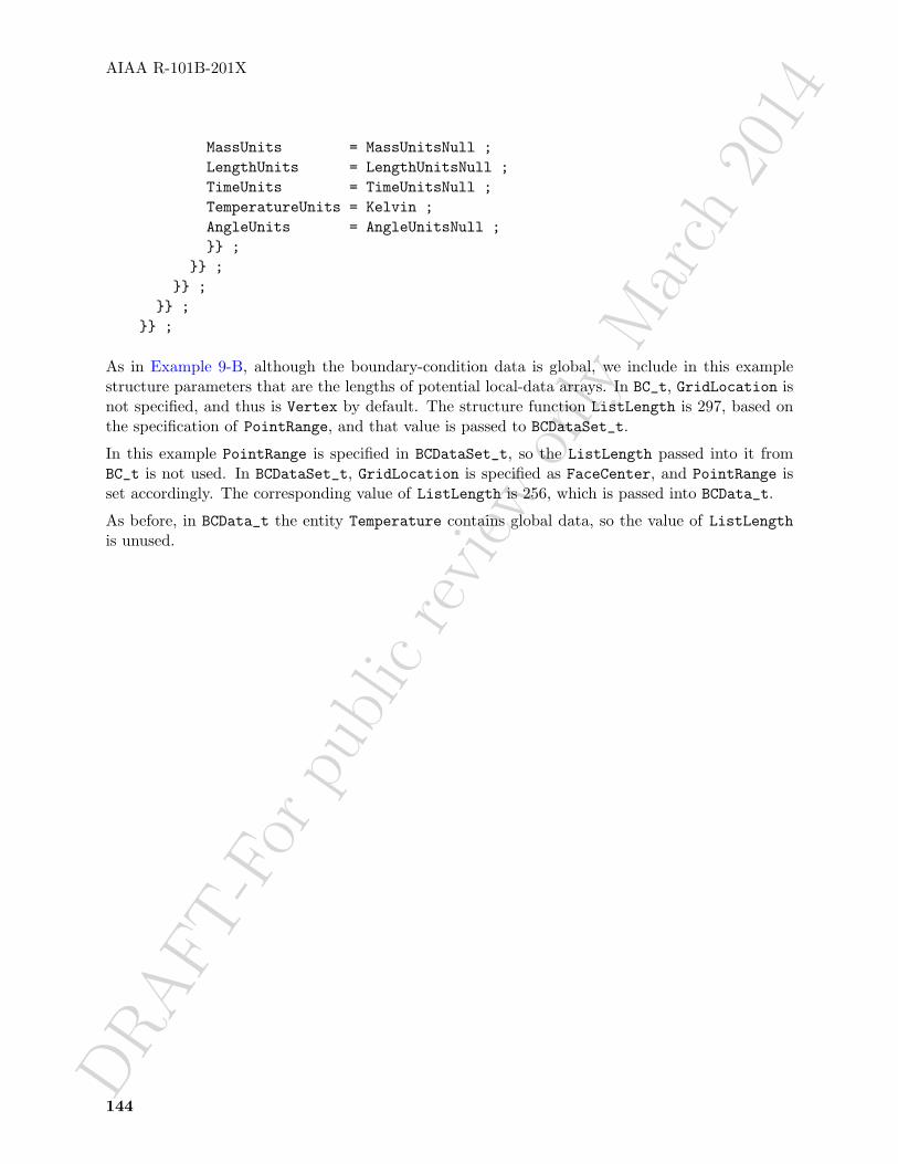
DRAFT

-For

publ

icre

view

only

Mar

ch20

14

AIAA R-101B-201X

MassUnits = MassUnitsNull ;LengthUnits = LengthUnitsNull ;TimeUnits = TimeUnitsNull ;TemperatureUnits = Kelvin ;AngleUnits = AngleUnitsNull ;}} ;

}} ;}} ;

}} ;}} ;

As in Example 9-B, although the boundary-condition data is global, we include in this examplestructure parameters that are the lengths of potential local-data arrays. In BC_t, GridLocation isnot specified, and thus is Vertex by default. The structure function ListLength is 297, based onthe specification of PointRange, and that value is passed to BCDataSet_t.

In this example PointRange is specified in BCDataSet_t, so the ListLength passed into it fromBC_t is not used. In BCDataSet_t, GridLocation is specified as FaceCenter, and PointRange isset accordingly. The corresponding value of ListLength is 256, which is passed into BCData_t.

As before, in BCData_t the entity Temperature contains global data, so the value of ListLengthis unused.

144

DRAFT-Forpublic

review

only


10 Governing Flow Equations

This section provides structure type definitions for describing the governing flow-equation set as-sociated with the database. The description includes the general class of governing equations, theturbulent closure equations, the gas and chemistry models, the viscosity and thermal-conductivitymodels, and the electromagnetics models. Included with each equation description are associatedconstants. The structure definitions attempt to balance the opposing requirements for future growthand extensibility with initial ease of implementation. Included in the final section (Section 10.11)are examples of flow-equation sets.

The intended use of these structures initially is primarily for archival purposes and to provideadditional documentation of the flow solution. If successful in this role, it is foreseeable that theseflow-equation structures may eventually be also used as inputs for grid generators, flow solvers, andpost-processors.

10.1 Flow Equation Set Structure Definition: FlowEquationSet_t

FlowEquationSet_t is a general description of the governing flow equations. It includes the dimen-sionality of the governing equations, and the collection of specific equation-set descriptions coveredin subsequent sections. It can be a child node of either CGNSBase_t or Zone_t (or both).

FlowEquationSet_t< int CellDimension > :={List( Descriptor_t Descriptor1 ... DescriptorN ) ; (o)

int EquationDimension ; (o)

GoverningEquations_t<CellDimension> GoverningEquations ; (o)

GasModel_t GasModel ; (o)

ViscosityModel_t ViscosityModel ; (o)

ThermalConductivityModel_t ThermalConductivityModel ; (o)

TurbulenceClosure_t TurbulenceClosure ; (o)

TurbulenceModel_t<CellDimension> TurbulenceModel ; (o)

ThermalRelaxationModel_t ThermalRelaxationModel ; (o)

ChemicalKineticsModel_t ChemicalKineticsModel ; (o)

EMElectricFieldModel_t EMElectricFieldModel ; (o)

145

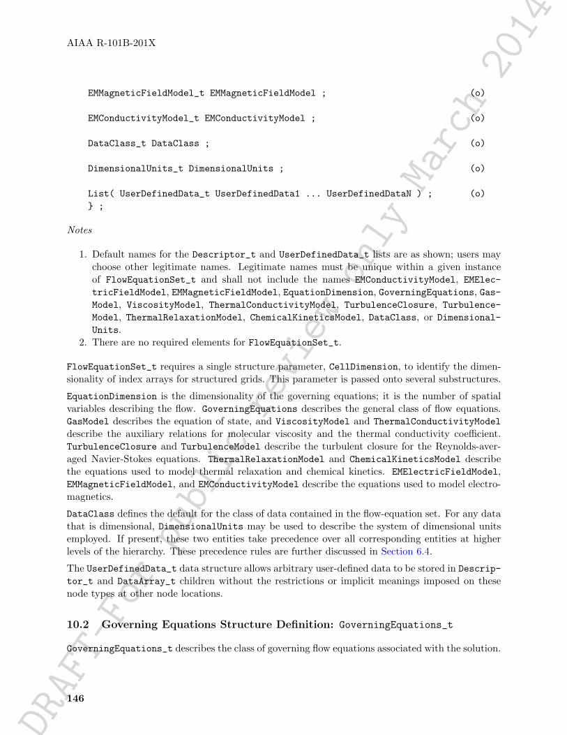
DRAFT-Forpublic

review

only


EMMagneticFieldModel_t EMMagneticFieldModel ; (o)

EMConductivityModel_t EMConductivityModel ; (o)




Notes

1. Default names for the Descriptor_t and UserDefinedData_t lists are as shown; users maychoose other legitimate names. Legitimate names must be unique within a given instanceof FlowEquationSet_t and shall not include the names EMConductivityModel, EMElec-tricFieldModel, EMMagneticFieldModel, EquationDimension, GoverningEquations, Gas-Model, ViscosityModel, ThermalConductivityModel, TurbulenceClosure, Turbulence-Model, ThermalRelaxationModel, ChemicalKineticsModel, DataClass, or Dimensional-Units.

2. There are no required elements for FlowEquationSet_t.

FlowEquationSet_t requires a single structure parameter, CellDimension, to identify the dimen-sionality of index arrays for structured grids. This parameter is passed onto several substructures.

EquationDimension is the dimensionality of the governing equations; it is the number of spatialvariables describing the flow. GoverningEquations describes the general class of flow equations.GasModel describes the equation of state, and ViscosityModel and ThermalConductivityModeldescribe the auxiliary relations for molecular viscosity and the thermal conductivity coefficient.TurbulenceClosure and TurbulenceModel describe the turbulent closure for the Reynolds-aver-aged Navier-Stokes equations. ThermalRelaxationModel and ChemicalKineticsModel describethe equations used to model thermal relaxation and chemical kinetics. EMElectricFieldModel,EMMagneticFieldModel, and EMConductivityModel describe the equations used to model electro-magnetics.

DataClass defines the default for the class of data contained in the flow-equation set. For any datathat is dimensional, DimensionalUnits may be used to describe the system of dimensional unitsemployed. If present, these two entities take precedence over all corresponding entities at higherlevels of the hierarchy. These precedence rules are further discussed in Section 6.4.


10.2 Governing Equations Structure Definition: GoverningEquations_t

GoverningEquations_t describes the class of governing flow equations associated with the solution.

146

DRAFT

-For

publ

icre

view

only

Mar

ch20

14

AIAA R-101B-201X

GoverningEquationsType_t := Enumeration(GoverningEquationsTypeNull,GoverningEquationsTypeUserDefined,FullPotential,Euler,NSLaminar,NSTurbulent,NSLaminarIncompressible,NSTurbulentIncompressible ) ;

GoverningEquations_t< int CellDimension > :={List( Descriptor_t Descriptor1 ... DescriptorN ) ; (o)

GoverningEquationsType_t GoverningEquationsType ; (r)

int[CellDimension*(CellDimension + 1)/2] DiffusionModel ; (o)


Notes

1. Default names for the Descriptor_t and UserDefinedData_t lists are as shown; users maychoose other legitimate names. Legitimate names must be unique within a given instance ofGoverningEquations_t and shall not include the name DiffusionModel.

2. GoverningEquationsType is the only required element.3. The length of the DiffusionModel array is as follows: in 1-D it is int[1]; in 2-D it is

int[3]; and in 3-D it is int[6]. For unstructured zones, DiffusionModel is not supported,and should not be used.

GoverningEquations_t requires a single structure parameter, CellDimension. It is used to definethe length of the array DiffusionModel.

DiffusionModel describes the viscous diffusion terms modeled in the flow equations, and is applica-ble only to the Navier-Stokes equations with structured grids. Typically, thin-layer approximationsinclude only the diffusion terms in one or two computational-coordinate directions. Diffusion-Model encodes the coordinate directions that include second-derivative and cross-derivative diffusionterms. The first CellDimension elements are second-derivative terms and the remainder elementsare cross-derivative terms. Allowed values for individual elements in the array DiffusionModelare 0 and 1; a value of 1 indicates the diffusion term is modeled, and 0 indicates that they are notmodeled. In 3-D, the encoding of DiffusionModel is as follows:

147

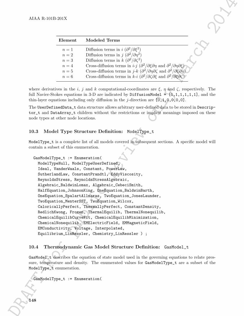
DRAFT-Forpublic

review

only


Element Modeled Terms

n = 1 Diffusion terms in i (∂2/∂ξ2)n = 2 Diffusion terms in j (∂2/∂η2)n = 3 Diffusion terms in k (∂2/∂ζ2)n = 4 Cross-diffusion terms in i-j (∂2/∂ξ∂η and ∂2/∂η∂ξ)n = 5 Cross-diffusion terms in j-k (∂2/∂η∂ζ and ∂2/∂ζ∂η)n = 6 Cross-diffusion terms in k-i (∂2/∂ζ∂ξ and ∂2/∂ξ∂ζ)

where derivatives in the i, j and k computational-coordinates are ξ, η and ζ, respectively. Thefull Navier-Stokes equations in 3-D are indicated by DiffusionModel = [1,1,1,1,1,1], and thethin-layer equations including only diffusion in the j-direction are [0,1,0,0,0,0].


10.3 Model Type Structure Definition: ModelType_t

ModelType_t is a complete list of all models covered in subsequent sections. A specific model willcontain a subset of this enumeration.

GasModelType_t := Enumeration(ModelTypeNull, ModelTypeUserDefined,Ideal, VanderWaals, Constant, PowerLaw,SutherlandLaw, ConstantPrandtl, EddyViscosity,ReynoldsStress, ReynoldsStressAlgebraic,Algebraic_BaldwinLomax, Algebraic_CebeciSmith,HalfEquation_JohnsonKing, OneEquation_BaldwinBarth,OneEquation_SpalartAllmaras, TwoEquation_JonesLaunder,TwoEquation_MenterSST, TwoEquation_Wilcox,CaloricallyPerfect, ThermallyPerfect, ConstantDensity,RedlichKwong, Frozen, ThermalEquilib, ThermalNonequilib,ChemicalEquilibCurveFit, ChemicalEquilibMinimization,ChemicalNonequilib, EMElectricField, EMMagneticField,EMConductivity, Voltage, Interpolated,Equilibrium_LinRessler, Chemistry_LinRessler ) ;

10.4 Thermodynamic Gas Model Structure Definition: GasModel_t

GasModel_t describes the equation of state model used in the governing equations to relate pres-sure, temperature and density. The enumerated values for GasModelType_t are a subset of theModelType_t enumeration.

GasModelType_t := Enumeration(

148

DRAFT

-For

publ

icre

view

only

Mar

ch20

14

AIAA R-101B-201X

ModelTypeNull,ModelTypeUserDefined,Ideal,VanderWaals,CaloricallyPerfect,ThermallyPerfect,ConstantDensity,RedlichKwong ) ;

GasModel_t :={List( Descriptor_t Descriptor1 ... DescriptorN ) ; (o)

GasModelType_t GasModelType ; (r)

List( DataArray_t<DataType, 1, 1> DataArray1 ... DataArrayN ) ; (o)




Notes

1. Default names for the Descriptor_t, DataArray_t, and UserDefinedData_t lists are asshown; users may choose other legitimate names. Legitimate names must be unique within agiven instance of GasModel_t and shall not include the names DataClass or Dimensional-Units.

2. GasModelType is the only required element.3. The GasModelType enumeration name Ideal implies a calorically perfect single-component

gas, but the more descriptive name CaloricallyPerfect is generally preferred.

For a perfect gas (GasModelType = CaloricallyPerfect), the pressure, temperature and densityare related by,

p = ρRT,

where R is the ideal gas constant. Related quantities are the specific heat at constant pressure (cp),specific heat at constant volume (cv) and specific heat ratio (γ = cp/cv). The gas constant andspecific heats are related by R = cp− cv. Data-name identifiers associated with the perfect gas laware listed in Table 5.

If it is desired to specify any of these identifiers in a CGNS database, they should be defined asDataArrays under GasModel_t.

149

DRAFT-Forpublic

review

only


Table 5: Data-Name Identifiers for Perfect Gas

Data-Name Identifier Description Units

IdealGasConstant Ideal gas constant (R) L2/(T2Θ)SpecificHeatRatio Ratio of specific heats (γ = cp/cv) -SpecificHeatVolume Specific heat at constant volume (cv) L2/(T2Θ)SpecificHeatPressure Specific heat at constant pressure (cp) L2/(T2Θ)

The dimensional units are defined as follows: M is mass, L is length, T is time and Θ is temperature.These are further described in Appendix A.

DataClass defines the default for the class of data contained in the thermodynamic gas model. Forany data that is dimensional, DimensionalUnits may be used to describe the system of dimensionalunits employed. If present, these two entities take precedence over all corresponding entities athigher levels of the hierarchy. These precedence rules are further discussed in Section 6.4.


10.5 Molecular Viscosity Model Structure Definition: ViscosityModel_t

ViscosityModel_t describes the model for relating molecular viscosity (µ) to temperature. Theenumerated values for ViscosityModelType_t are a subset of the ModelType_t enumeration.

ViscosityModelType_t := Enumeration(ModelTypeNull,ModelTypeUserDefined,Constant,PowerLaw,SutherlandLaw ) ;

ViscosityModel_t :={List( Descriptor_t Descriptor1 ... DescriptorN ) ; (o)

ViscosityModelType_t ViscosityModelType ; (r)




150

DRAFT

-For

publ

icre

view

only

Mar

ch20

14

AIAA R-101B-201X


Notes

1. Default names for the Descriptor_t, DataArray_t, and UserDefinedData_t lists are asshown; users may choose other legitimate names. Legitimate names must be unique within agiven instance of ViscosityModel_t and shall not include the names DataClass or Dimen-sionalUnits.

2. ViscosityModelType is the only required element.

The molecular viscosity models are as follows: Constant states that molecular viscosity is constantthroughout the field and is equal to some reference value (µ = µref); PowerLaw states that molecularviscosity follows a power-law relation,

µ = µref

(T

Tref

)nand SutherlandLaw is Sutherland’s Law for molecular viscosity,

µ = µref

(T

Tref

)3/2 Tref + TsT + Ts

,

where Ts is the Sutherland’s Law constant, and µref and Tref are the reference viscosity and tem-perature, respectively. For air3, the power-law exponent is n = 0.666, Sutherland’s law constant(Ts) is 110.6 K, the reference temperature (Tref) is 273.15 K, and the reference viscosity (µref)is 1.716×10−5 kg/(m-s). The data-name identifiers for molecular viscosity models are defined inTable 6.

Table 6: Data-Name Identifiers for Molecular Viscosity Models

ViscosityModelType Data-Name Identifer Description Units

PowerLaw PowerLawExponent Power-law exponent (n) -SutherlandLaw SutherlandLawConstant Sutherland’s Law

constant (Ts)Θ

All TemperatureReference Reference temperature(Tref)

Θ

All ViscosityMolecularReference Reference viscosity (µref) M/(LT)

If it is desired to specify any of these identifiers in a CGNS database, they should be defined asDataArrays under ViscosityModel_t.

3White, F. M., Viscous Fluid Flow, McGraw-Hill, 1974, p. 28-29

151

DRAFT

-For

publ

icre

view

only

Mar

ch20

14

AIAA R-101B-201X

DataClass defines the default for the class of data contained in the molecular viscosity model. Forany data that is dimensional, DimensionalUnits may be used to describe the system of dimensionalunits employed. If present, these two entities take precedence over all corresponding entities athigher levels of the hierarchy. These precedence rules are further discussed in Section 6.4.


10.6 Thermal Conductivity Model Structure Definition: ThermalConductivity-

Model_t

ThermalConductivityModel_t describes the model for relating the thermal-conductivity coefficient(k) to temperature. The enumerated values for ThermalConductivityModelType_t are a subsetof the ModelType_t enumeration.

ThermalConductivityModelType_t := Enumeration(ModelTypeNull,ModelTypeUserDefined,ConstantPrandtl,PowerLaw,SutherlandLaw ) ;

ThermalConductivityModel_t :={List( Descriptor_t Descriptor1 ... DescriptorN ) ; (o)

ThermalConductivityModelType_t ThermalConductivityModelType ; (r)





Notes

1. Default names for the Descriptor_t and DataArray_t UserDefinedData_t lists are asshown; users may choose other legitimate names. Legitimate names must be unique within agiven instance of ThermalConductivityModel_t and shall not include the names DataClassor DimensionalUnits.

2. ThermalConductivityModelType is the only required element.

152

DRAFT

-For

publ

icre

view

only

Mar

ch20

14

AIAA R-101B-201X

The thermal-conductivity models parallel the molecular viscosity models. ConstantPrandtl statesthat the Prandtl number (Pr = µcp/k) is constant and equal to some reference value. PowerLawrelates k to temperature via a power-law relation,

k = kref

(T

Tref

)n.

SutherlandLaw states the Sutherland’s Law for thermal conductivity,

k = kref

(T

Tref

)3/2 Tref + TsT + Ts

,

where kref is the reference thermal conductivity, Tref is the reference temperature, and Ts is theSutherland’s law constant. For air4, the Prandtl number is Pr = 0.72, the power-law exponent isn = 0.81, Sutherland’s law constant (Ts) is 194.4 K, the reference temperature (Tref) is 273.15 K,and the reference thermal conductivity (kref) is 2.414×10−2 kg-m/(s3-K). Data-name identifiers forthermal conductivity models are listed in Table 7.

Table 7: Data-Name Identifiers for Thermal Conductivity Models

ThermalConduc-tivityModelType

Data-Name Identifer Description Units

ConstantPrandtl Prandtl Prandtl number (Pr) -PowerLaw PowerLawExponent Power-law exponent (n) -SutherlandLaw SutherlandLawConstant Sutherland’s Law

constant (Ts)Θ

All TemperatureReference Reference temperature(Tref)

Θ

All ThermalConductivityReference Reference thermalconductivity (kref)

ML/(T3Θ)

If it is desired to specify any of these identifiers in a CGNS database, they should be defined asDataArrays under ThermalConductivityModel_t.

DataClass defines the default for the class of data contained in the thermal conductivity model. Forany data that is dimensional, DimensionalUnits may be used to describe the system of dimensionalunits employed. If present, these two entities take precedence over all corresponding entities athigher levels of the hierarchy. These precedence rules are further discussed in Section 6.4.


4White, F. M., Viscous Fluid Flow, McGraw-Hill, 1974, p. 32-33

153

DRAFT

-For

publ

icre

view

only

Mar

ch20

14

AIAA R-101B-201X

10.7 Turbulence Structure Definitions

This section presents structure definitions for describing the form of closure used in the Reynolds-averaged (or Favre-averaged) Navier-Stokes equations for determining the Reynolds stress terms.Here “turbulence closure” refers to eddy viscosity or other approximations for the Reynolds stressterms, and “turbulence model” refers to the actual algebraic or turbulence-transport equation mod-els used. To an extent these are independent choices (e.g., using either an eddy viscosity closure oran algebraic Reynolds-stress closure with a two-equation model).

10.7.1 Turbulence Closure Structure Definition: TurbulenceClosure_t

TurbulenceClosure_t describes the turbulence closure for the Reynolds stress terms of the Navier-Stokes equations. The enumerated values for TurbulenceClosureType_t are a subset of the Mod-elType_t enumeration.

TurbulenceClosureType_t := Enumeration(ModelTypeNull,ModelTypeUserDefined,EddyViscosity,ReynoldsStress,ReynoldsStressAlgebraic ) ;

TurbulenceClosure_t :={List( Descriptor_t Descriptor1 ... DescriptorN ) ; (o)

TurbulenceClosureType_t TurbulenceClosureType ; (r)





Notes

1. Default names for the Descriptor_t, DataArray_t, and UserDefinedData_t lists are asshown; users may choose other legitimate names. Legitimate names must be unique withina given instance of TurbulenceClosure_t and shall not include the names DataClass orDimensionalUnits.

2. TurbulenceClosureType is the only required element.

154

DRAFT-Forpublic

review

only


The different types of turbulent closure are as follows: EddyViscosity is the Boussinesq eddy-viscosity closure, where the Reynolds stresses are approximated as the product of an eddy viscosity(νt) and the mean strain tensor. Using indicial notation, the relation is,

−u′iu′j = νt

(∂ui∂xj

+∂uj∂xi

),

where −u′iu′j are the Reynolds stresses; the notation is further discussed in Appendix A.2. Rey-noldsStress is no approximation of the Reynolds stresses. ReynoldsStressAlgebraic is an alge-braic approximation for the Reynolds stresses based on some intermediate transport quantities.

Associated with the turbulent closure is a list of constants, where each constant is described bya separate DataArray_t entity. Constants associated with the eddy-viscosity closure are listed inTable 8.

Table 8: Data-Name Identifiers for Turbulence Closure


PrandtlTurbulent Turbulent Prandtl number (ρνtcp/kt) -

If it is desired to specify any of these identifiers in a CGNS database, they should be defined asDataArrays under TurbulenceClosure_t.

DataClass defines the default for the class of data contained in the turbulence closure. For anydata that is dimensional, DimensionalUnits may be used to describe the system of dimensionalunits employed. If present, these two entities take precedence over all corresponding entities athigher levels of the hierarchy. These precedence rules are further discussed in Section 6.4.


10.7.2 Turbulence Model Structure Definition: TurbulenceModel_t

TurbulenceModel\_t describes the equation set used to model the turbulence quantities. Theenumerated values for TurbulenceModelType_t are a subset of the ModelType_t enumeration.

TurbulenceModelType_t := Enumeration(ModelTypeNull,ModelTypeUserDefined,Algebraic_BaldwinLomax,Algebraic_CebeciSmith,HalfEquation_JohnsonKing,OneEquation_BaldwinBarth,OneEquation_SpalartAllmaras,

155

DRAFT

-For

publ

icre

view

only

Mar

ch20

14

AIAA R-101B-201X

TwoEquation_JonesLaunder,TwoEquation_MenterSST,TwoEquation_Wilcox ) ;

TurbulenceModel_t< int CellDimension > :={List( Descriptor_t Descriptor1 ... DescriptorN ) ; (o)

TurbulenceModelType_t TurbulenceModelType ; (r)


int[CellDimension*(CellDimension + 1)/2] DiffusionModel ; (o)




Notes

1. Default names for the Descriptor_t and DataArray_t UserDefinedData_t lists are asshown; users may choose other legitimate names. Legitimate names must be unique withina given instance of TurbulenceModel_t and shall not include the names DiffusionModel,DataClass, or DimensionalUnits.

2. TurbulenceModelType is the only required element.3. The length of the DiffusionModel array is as follows: in 1-D it is int[1]; in 2-D it is

int[3]; and in 3-D it is int[6]. For unstructured zones, DiffusionModel is not supported,and should not be used.

TurbulenceModel_t requires a single structure parameter, CellDimension. It is used to definethe length of the array DiffusionModel. DiffusionModel describes the viscous diffusion termsincluded in the turbulent transport model equations; the encoding of DiffusionModel is describedin Section 10.2.

The TurbulenceModelType names currently listed correspond to the following particular references.

Algebraic_BaldwinLomax Baldwin, B. S., and Lomax, H. (1978) “Thin Layer Ap-proximations and Algebraic Model for Separated TurbulentFlows,” AIAA Paper 78-257.

Algebraic_CebeciSmith Cebeci, T., and Smith, A. M. O. (1974) Analysis of Turbu-lent Boundary Layers, Academic Press, New York.

156

DRAFT-Forpublic

review

only


HalfEquation_JohnsonKing Johnson, D., and King, L. (1985) “A Mathematically Sim-ple Turbulence Closure Model for Attached and SeparatedTurbulent Boundary Layers,” AIAA Journal, Vol. 23, No.11, pp. 1684–1692.

OneEquation_BaldwinBarth Baldwin, B., and Barth, T. (1990) “A One-Equation Tur-bulent Transport Model for High Reynolds Number Wall-Bounded Flows,” NASA TM-102847.

OneEquation_SpalartAllmaras Spalart, P. R., and Allmaras, S. R. (1994) “A One-EquationTurbulence Model for Aerodynamic Flows,” La RechercheAerospatiale, Vol. 1, pp. 5–21.

TwoEquation_JonesLaunder Jones, W., and Launder, B. (1972) “The Prediction of Lam-inarization with a Two-Equation Model of Turbulence,” In-ternational Journal of Heat and Mass Transfer, Vol. 15, pp.301–314.

TwoEquation_MenterSST Menter, F. R. (1994)“Two-Equation Eddy-Viscosity Turbu-lence Models for Engineering Application,” AIAA Journal,Vol. 32, No. 8, pp. 1598–1605.

TwoEquation_Wilcox Wilcox, D. C. (1994) Turbulence Modeling for CFD, FirstEdition, DCW Industries, La Canada, California.

There is no formal mechanism for accounting for subsequent changes to these models. (For exam-ple, Wilcox later published 1998 and 2006 versions of his k-ω model). If it is a mere change toconstant(s), then this could be described by retaining the same TurbulenceModelType name andlisting each constant using a separate DataArray_t entry. If the change is more involved, then it isrecommended to employ TurbulenceModelType = UserDefined with a child Descriptor_t nodegiving details about it.

Associated with each choice of turbulence model may be a list of constants, where each constantis described by a separate DataArray_t entity. If used, the Data-Name Identifier of each constantshould include the turbulence model name, as well as the constant name (e.g., TurbulentSACb1,TurbulentSSTCmu, TurbulentKESigmak, etc.). However, no attempt is made here to formalize thenames for all possible turbulence models.

DataClass defines the default for the class of data contained in the turbulence model equationset. For any data that is dimensional, DimensionalUnits may be used to describe the system ofdimensional units employed. If present, these two entities take precedence over all correspondingentities at higher levels of the hierarchy. These precedence rules are further discussed in Section 6.4.


Example 10-A: Spalart-Allmaras Turbulence Model

157

DRAFT-Forpublic

review

only


Description for the eddy-viscosity closure and Spalart-Allmaras turbulence model, including asso-ciated constants.

TurbulenceClosure_t TurbulenceClosure ={{TurbulenceClosureType_t TurbulenceClosureType = EddyViscosity ;

DataArray_t<real, 1, 1> PrandtlTurbulent = {{ 0.90 }} ;}} ;

TurbulenceModel_t TurbulenceModel ={{TurbulenceModelType_t TurbulenceModelType = OneEquation_SpalartAllmaras ;

DataArray_t<real, 1, 1> TurbulentSACb1 = {{ 0.1355 }} ;DataArray_t<real, 1, 1> TurbulentSACb2 = {{ 0.622 }} ;DataArray_t<real, 1, 1> TurbulentSASigma = {{ 2/3 }} ;DataArray_t<real, 1, 1> TurbulentSAKappa = {{ 0.41 }} ;DataArray_t<real, 1, 1> TurbulentSACw1 = {{ 3.2391 }} ;DataArray_t<real, 1, 1> TurbulentSACw2 = {{ 0.3 }} ;DataArray_t<real, 1, 1> TurbulentSACw3 = {{ 2 }} ;DataArray_t<real, 1, 1> TurbulentSACv1 = {{ 7.1 }} ;DataArray_t<real, 1, 1> TurbulentSACt1 = {{ 1 }} ;DataArray_t<real, 1, 1> TurbulentSACt2 = {{ 2 }} ;DataArray_t<real, 1, 1> TurbulentSACt3 = {{ 1.2 }} ;DataArray_t<real, 1, 1> TurbulentSACt4 = {{ 0.5 }} ;}} ;

Note that each DataArray_t entity is abbreviated.

10.8 Thermal Relaxation Model Structure Definition: ThermalRelaxationMod-

elType_t

ThermalRelaxationModel_t describes the equation set used to model thermal relaxation quanti-ties. The enumerated values for ThermalRelaxationModelType_t are a subset of the ModelType_tenumeration.

ThermalRelaxationModelType_t := Enumeration(ModelTypeNull,ModelTypeUserDefined,Frozen,ThermalEquilib,ThermalNonequilib ) ;

ThermalRelaxationModel_t :=

158

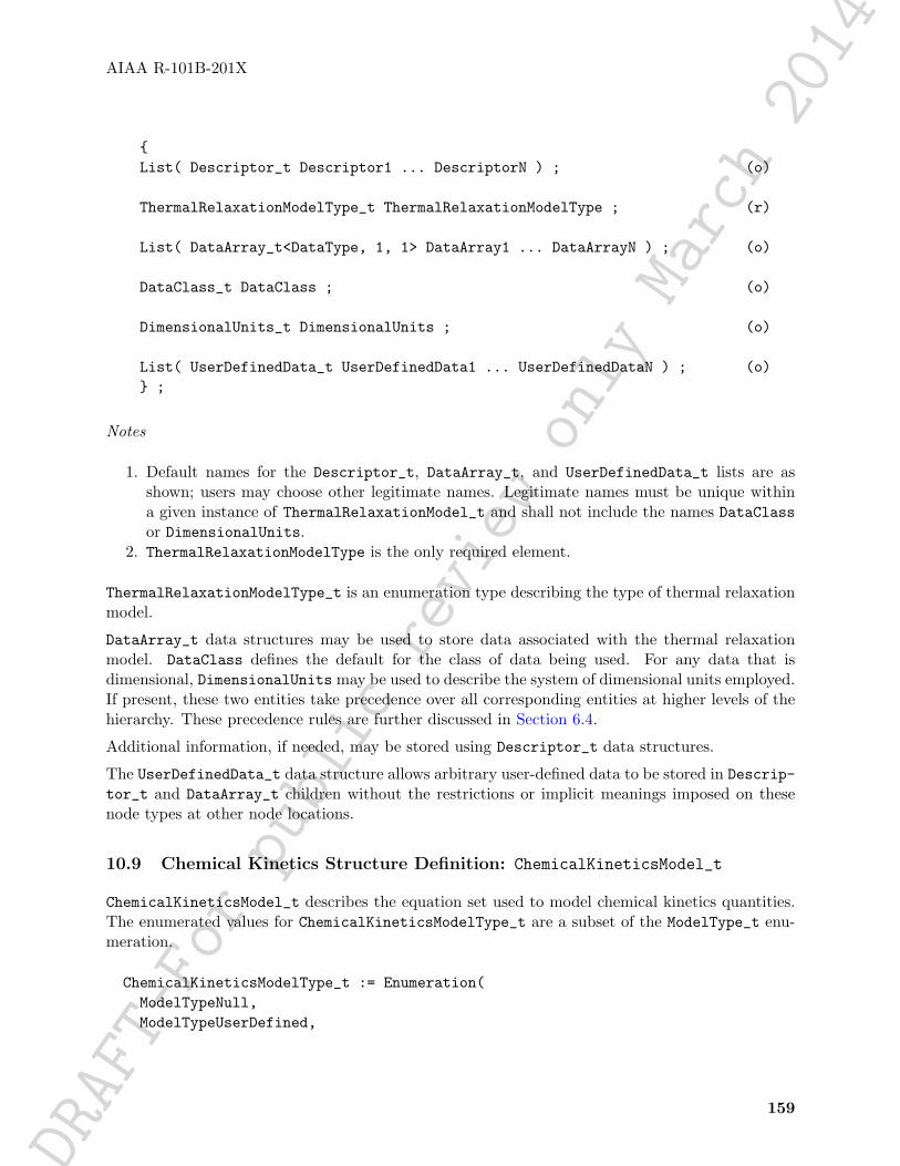
DRAFT-Forpublic

review

only



ThermalRelaxationModelType_t ThermalRelaxationModelType ; (r)





Notes

1. Default names for the Descriptor_t, DataArray_t, and UserDefinedData_t lists are asshown; users may choose other legitimate names. Legitimate names must be unique withina given instance of ThermalRelaxationModel_t and shall not include the names DataClassor DimensionalUnits.

2. ThermalRelaxationModelType is the only required element.

ThermalRelaxationModelType_t is an enumeration type describing the type of thermal relaxationmodel.

DataArray_t data structures may be used to store data associated with the thermal relaxationmodel. DataClass defines the default for the class of data being used. For any data that isdimensional, DimensionalUnits may be used to describe the system of dimensional units employed.If present, these two entities take precedence over all corresponding entities at higher levels of thehierarchy. These precedence rules are further discussed in Section 6.4.

Additional information, if needed, may be stored using Descriptor_t data structures.


10.9 Chemical Kinetics Structure Definition: ChemicalKineticsModel_t

ChemicalKineticsModel_t describes the equation set used to model chemical kinetics quantities.The enumerated values for ChemicalKineticsModelType_t are a subset of the ModelType_t enu-meration.

ChemicalKineticsModelType_t := Enumeration(ModelTypeNull,ModelTypeUserDefined,

159

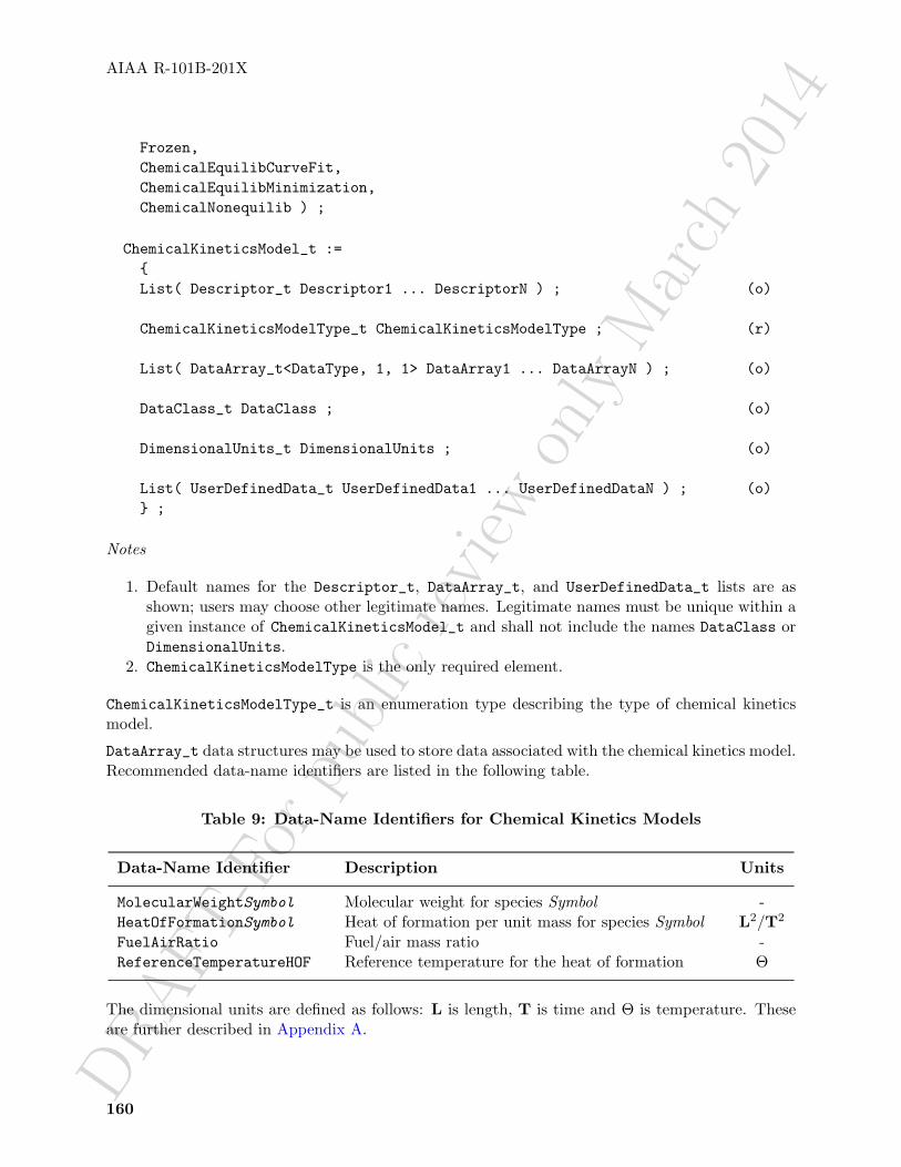
DRAFT

-For

publ

icre

view

only

Mar

ch20

14

AIAA R-101B-201X

Frozen,ChemicalEquilibCurveFit,ChemicalEquilibMinimization,ChemicalNonequilib ) ;

ChemicalKineticsModel_t :={List( Descriptor_t Descriptor1 ... DescriptorN ) ; (o)

ChemicalKineticsModelType_t ChemicalKineticsModelType ; (r)





Notes

1. Default names for the Descriptor_t, DataArray_t, and UserDefinedData_t lists are asshown; users may choose other legitimate names. Legitimate names must be unique within agiven instance of ChemicalKineticsModel_t and shall not include the names DataClass orDimensionalUnits.

2. ChemicalKineticsModelType is the only required element.

ChemicalKineticsModelType_t is an enumeration type describing the type of chemical kineticsmodel.

DataArray_t data structures may be used to store data associated with the chemical kinetics model.Recommended data-name identifiers are listed in the following table.

Table 9: Data-Name Identifiers for Chemical Kinetics Models


MolecularWeightSymbol Molecular weight for species Symbol -HeatOfFormationSymbol Heat of formation per unit mass for species Symbol L2/T2

FuelAirRatio Fuel/air mass ratio -ReferenceTemperatureHOF Reference temperature for the heat of formation Θ

The dimensional units are defined as follows: L is length, T is time and Θ is temperature. Theseare further described in Appendix A.

160

DRAFT

-For

publ

icre

view

only

Mar

ch20

14

AIAA R-101B-201X

The variable string Symbol in the above data-name identifiers represents the chemical symbolfor the desired species. For example, H represents hydrogen atoms, O represents oxygen atoms,H2 represents hydrogen molecules, H2O represents water molecules, and C3H5O3(NO2)3 representsnitroglycerin molecules. Any symbols from the periodic table of the elements can be used. Forcharged molecules or particles, the word “plus” or “minus” should be spelled out in lower case. Forexample, a CNO+ molecule should be denoted as CNOplus.

Other commonly used mixtures, that are usually not referred to by their chemical symbols, aredefined in the following table. Individual users may define new names, but these may not berecognized by other CGNS applications. For consistency, additional names should be proposed asSIDS extensions.

Table 10: Defined Names (Symbols) for Commonly Used Mixtures

Symbol Mixture

Air Generic air modeleminus ElectronsFuel Generic fuel modelFuelAir Generic fuel/air mixtureJP5 JP5 jet fuelJP7 JP7 jet fuelJP10 JP10 jet fuelProduct Generic fuel/air product of combustionRP1 RP1 rocket fuel

DataClass defines the default for the class of data being used. For any data that is dimensional,DimensionalUnits may be used to describe the system of dimensional units employed. If present,these two entities take precedence over all corresponding entities at higher levels of the hierarchy,following the standard precedence rules.

Additional information, if needed, may be stored using Descriptor_t data structures. For example,if CHEMKIN is used, it is recommended that a Descriptor_t data structure be used to indicatethis. Reaction equations could also be specified using Descriptor_t data structures.


10.10 Electromagnetics Structure Definitions

This section presents structure definitions for describing the electric field, magnetic field, and con-ductivity models used for electromagnetic flows.

161

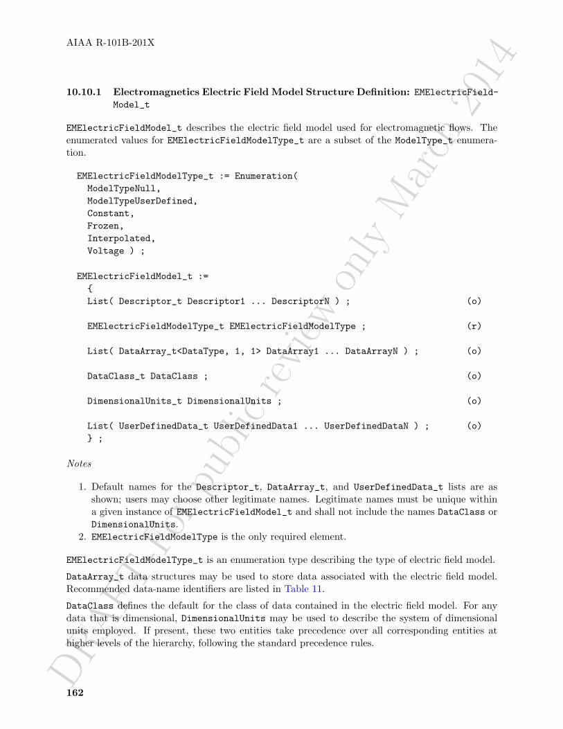
DRAFT

-For

publ

icre

view

only

Mar

ch20

14

AIAA R-101B-201X

10.10.1 Electromagnetics Electric Field Model Structure Definition: EMElectricField-Model_t

EMElectricFieldModel_t describes the electric field model used for electromagnetic flows. Theenumerated values for EMElectricFieldModelType_t are a subset of the ModelType_t enumera-tion.

EMElectricFieldModelType_t := Enumeration(ModelTypeNull,ModelTypeUserDefined,Constant,Frozen,Interpolated,Voltage ) ;

EMElectricFieldModel_t :={List( Descriptor_t Descriptor1 ... DescriptorN ) ; (o)

EMElectricFieldModelType_t EMElectricFieldModelType ; (r)





Notes

1. Default names for the Descriptor_t, DataArray_t, and UserDefinedData_t lists are asshown; users may choose other legitimate names. Legitimate names must be unique withina given instance of EMElectricFieldModel_t and shall not include the names DataClass orDimensionalUnits.

2. EMElectricFieldModelType is the only required element.

EMElectricFieldModelType_t is an enumeration type describing the type of electric field model.

DataArray_t data structures may be used to store data associated with the electric field model.Recommended data-name identifiers are listed in Table 11.

DataClass defines the default for the class of data contained in the electric field model. For anydata that is dimensional, DimensionalUnits may be used to describe the system of dimensionalunits employed. If present, these two entities take precedence over all corresponding entities athigher levels of the hierarchy, following the standard precedence rules.

162

DRAFT

-For

publ

icre

view

only

Mar

ch20

14

AIAA R-101B-201X


10.10.2 Electromagnetics Magnetic Field Model Structure Definition: EMMagnetic-FieldModel_t

EMMagneticFieldModel_t describes the magnetic field model used for electromagnetic flows. Theenumerated values for EMMagneticFieldModelType_t are a subset of the ModelType_t enumera-tion.

EMMagneticFieldModelType_t := Enumeration(ModelTypeNull,ModelTypeUserDefined,Constant,Frozen,Interpolated ) ;

EMMagneticFieldModel_t :={List( Descriptor_t Descriptor1 ... DescriptorN ) ; (o)

EMMagneticFieldModelType_t EMMagneticFieldModelType ; (r)





Notes

1. Default names for the Descriptor_t, DataArray_t, and UserDefinedData_t lists are asshown; users may choose other legitimate names. Legitimate names must be unique withina given instance of EMMagneticFieldModel_t and shall not include the names DataClass orDimensionalUnits.

2. EMMagneticFieldModelType is the only required element.

EMMagneticFieldModelType_t is an enumeration type describing the type of magnetic field model.

DataArray_t data structures may be used to store data associated with the magnetic field model.Recommended data-name identifiers are listed in Table 11.

163

DRAFT

-For

publ

icre

view

only

Mar

ch20

14

AIAA R-101B-201X

DataClass defines the default for the class of data contained in the electric field model. For anydata that is dimensional, DimensionalUnits may be used to describe the system of dimensionalunits employed. If present, these two entities take precedence over all corresponding entities athigher levels of the hierarchy, following the standard precedence rules.


10.10.3 Electromagnetics Conductivity Model Structure Definition: EMConductivity-Model_t

EMConductivityModel_t describes the conductivity model used for electromagnetic flows. Theenumerated values for EMConductivityModelType_t are a subset of the ModelType_t enumeration.

EMConductivityModelType_t := Enumeration(ModelTypeNull,ModelTypeUserDefined,Constant,Frozen,Equilibrium_LinRessler,Chemistry_LinRessler ) ;

EMConductivityModel_t :={List( Descriptor_t Descriptor1 ... DescriptorN ) ; (o)

EMConductivityModelType_t EMConductivityModelType ; (r)





Notes

1. Default names for the Descriptor_t, DataArray_t, and UserDefinedData_t lists are asshown; users may choose other legitimate names. Legitimate names must be unique withina given instance of EMConductivityModel_t and shall not include the names DataClass orDimensionalUnits.

2. EMConductivityModelType is the only required element.

164

DRAFT-Forpublic

review

only


EMConductivityModelType_t is an enumeration type describing the type of conductivity model.

DataArray_t data structures may be used to store data associated with the conductivity model.Recommended data-name identifiers are listed in Table 11.

Table 11: Data-Name Identifiers for Electromagnetics Models


Voltage Voltage ML2/TIElectricFieldX x-component of electric field vector ML/TIElectricFieldY y-component of electric field vector ML/TIElectricFieldZ z-component of electric field vector ML/TIMagneticFieldX x-component of magnetic field vector I/LMagneticFieldY y-component of magnetic field vector I/LMagneticFieldZ z-component of magnetic field vector I/LCurrentDensityX x-component of current density vector I/L2

CurrentDensityY y-component of current density vector I/L2

CurrentDensityZ z-component of current density vector I/L2

ElectricConductivity Electrical conductivity ML/T3I2

LorentzForceX x-component of Lorentz force vector ML/T2

LorentzForceY y-component of Lorentz force vector ML/T2

LorentzForceZ z-component of Lorentz force vector ML/T2

JouleHeating Joule heating ML2/T2

The dimensional units are defined as follows: M is mass, L is length, T is time, and I is electriccurrent. These are further described in Appendix A.

DataClass defines the default for the class of data contained in the conductivity model. For anydata that is dimensional, DimensionalUnits may be used to describe the system of dimensionalunits employed. If present, these two entities take precedence over all corresponding entities athigher levels of the hierarchy, following the standard precedence rules.


10.11 Flow Equation Examples

This section presents two examples of flow-equation sets. The first is an inviscid case and the secondis a turbulent case with a one-equation turbulence model.

Example 10-B: 3-D Compressible Euler

3-D compressible Euler with a perfect gas assumption for a monatomic gas:

FlowEquationSet_t<3> EulerEquations =

165

DRAFT-Forpublic

review

only


{{int EquationDimension = 3 ;

GoverningEquations_t<3> GoverningEquations ={{GoverningEquationsType_t GoverningEquationsType = Euler ;}} ;

GasModel_t GasModel ={{GasModelType_t GasModelType = CaloricallyPerfect ;

DataArray_t<real, 1, 1> SpecificHeatRatio ={{Data(real, 1, 1) = 1.667 ;

DataClass_t DataClass = NondimensionalParameter ;}} ;

}} ;}} ;

Example 10-C: 3-D Compressible Navier-Stokes

3-D compressible Navier-Stokes for a structured grid, with the S-A turbulence model, a perfect gasassumption, Sutherland’s law for the molecular viscosity, a constant Prandtl-number assumption,and inclusion of the full Navier-Stokes diffusion terms; all models assume air:

FlowEquationSet_t<3> NSEquations ={{int EquationDimension = 3 ;

GoverningEquations_t<3> GoverningEquations ={{GoverningEquationsType_t GoverningEquationsType = NSTurbulent ;

int[6] DiffusionModel = [1,1,1,1,1,1] ;}} ;


DataArray_t<real, 1, 1> SpecificHeatRatio = {{ 1.4 }} ;}} ;

166

DRAFT

-For

publ

icre

view

only

Mar

ch20

14

AIAA R-101B-201X

ViscosityModel_t ViscosityModel ={{ViscosityModelType_t ViscosityModelType = SutherlandLaw ;

DataArray_t<real, 1, 1> SutherlandLawConstant ={{Data(real, 1, 1) = 110.6 }} ;

DataClass_t DataClass = Dimensional ;DimensionalUnits_t DimensionalUnits = {{ TemperatureUnits = Kelvin }} ;}} ;

}} ;

ThermalConductivityModel_t ThermalConductivityModel ={{ThermalConductivityModelType_t ThermalConductivityModelType =

ConstantPrandtl ;

DataArray_t<real, 1, 1> Prandtl = {{ 0.72 }} ;}} ;

TurbulenceClosure_t<3> TurbulenceClosure ={{TurbulenceClosureType_t TurbulenceClosureType = EddyViscosity ;

DataArray_t<real, 1, 1> PrandtlTurbulent = {{ 0.90 }} ;}} ;

TurbulenceModel_t<3> TurbulenceModel ={{TurbulenceModelType_t TurbulenceModelType = OneEquation_SpalartAllmaras ;


}} ;

Note that all DataArray_t entities are abbreviated except SutherlandLawConstant.

167

DRAFT

-For

publ

icre

view

only

Mar

ch20

14

DRAFT

-For

publ

icre

view

only

Mar

ch20

14

AIAA R-101B-201X

11 Time-Dependent Flow

This section describes structure types intended primarily for time-dependent flows. Data structuresare presented for storing time-dependent or iterative data, and for recording rigid and arbitary gridmotion. The section concludes with several examples.

11.1 Iterative Data Structure Definitions

In order to keep a record of time dependent or iterative data, the data structures BaseIterative-Data_t and ZoneIterativeData_t are used.

11.1.1 Base Iterative Data Structure Definition: BaseIterativeData_t

The BaseIterativeData_t data structure is located directly under the CGNSBase_t node. It con-tains information about the number of time steps or iterations being recorded, and the time and/oriteration values at each step. In addition, it may include the list of zones and families for each stepof the simulation, if these vary throughout the simulation.

The BaseIterativeData_t data structure is defined as follows:

BaseIterativeData_t :={int NumberOfSteps (r)

DataArray_t<real, 1, NumberOfSteps> TimeValues ; (o/r)DataArray_t<int, 1, NumberOfSteps> IterationValues ; (r/o)

DataArray_t<int, 1, NumberOfSteps> NumberOfZones ; (o)DataArray_t<int, 1, NumberOfSteps> NumberOfFamilies ; (o)DataArray_t<char, 3, [32, MaxNumberOfZones, NumberOfSteps]>

ZonePointers ; (o)DataArray_t<char, 3, [32, MaxNumberOfFamilies, NumberOfSteps]>

FamilyPointers ; (o)

List( DataArray_t<> DataArray1 ... DataArrayN ) ; (o)

List( Descriptor_t Descriptor1 ... DescriptorN ) ; (o)



List( UserDefinedData_t UserDefinedData1 ... UserDefinedDataN ) ; (o)}

169

DRAFT-Forpublic

review

only


Notes

1. Default names for the DataArray_t, Descriptor_t, and UserDefinedData_t lists are asshown; users may choose other legitimate names. Legitimate names must be unique withina given instance of BaseIterativeData_t and shall not include the names DataClass, Di-mensionalUnits, FamilyPointers, IterationValues, NumberOfFamilies, NumberOfZones,TimeValues, or ZonePointers.

2. NumberOfSteps is a required element of the BaseIterativeData_t data structure. It holdseither the number of time steps or the number of iterations being recorded.

3. Either TimeValues or IterationValues must be defined. If both are used, there must be aone-to-one correspondence between them.

TimeValues and IterationValues are data-name identifiers corresponding to the time and iter-ation values stored in the file. When IterationValues are used, the iterative data stored in thedatabase correspond to values at the end of the associated iteration.

The data-name identifiers NumberOfZones and ZonePointers are only used if different zone datastructures apply to different steps of the simulation. (See Example 11-C.)

Similarly, if the geometry varies with time or iteration, then the data-name identifiers NumberOf-Families and FamilyPointers are used to record which Family_t data structure(s) correspond(s)to which step.

The DataArray_t nodes for ZonePointers and FamilyPointers are defined as three-dimensionalarrays. For each recorded step, the names of all zones and families being used for the step maybe recorded. Note that the names are limited to 32 characters, as usual in the SIDS. The vari-ables MaxNumberOfZones and MaxNumberOfFamilies represent the maximum number of zones andfamilies that apply to one step. So if NumberOfSteps = 5 and NumberOfZones = {2,2,3,4,3}, thenMaxNumberOfZones equals 4.

When NumberOfZones and NumberOfFamilies vary for different stored time steps, the name Nullis used in ZonePointers and FamilyPointers as appropriate for steps in which the NumberOfZonesor NumberOfFamilies is less than the MaxNumberOfZones or MaxNumberOfFamilies.

Any number of extra DataArray_t nodes are allowed. These should be used to record data notcovered by this specification.

11.1.2 Zone Iterative Data Structure Definition: ZoneIterativeData_t

The ZoneIterativeData_t data structure is located under the Zone_t node. It may be used torecord pointers to zonal data for each recorded step of the simulation, and is defined as follows:

ZoneIterativeData_t< int NumberOfSteps > :={DataArray_t<char, 2, [32, NumberOfSteps]> RigidGridMotionPointers ; (o)DataArray_t<char, 2, [32, NumberOfSteps]> ArbitraryGridMotionPointers ; (o)DataArray_t<char, 2, [32, NumberOfSteps]> GridCoordinatesPointers ; (o)DataArray_t<char, 2, [32, NumberOfSteps]> FlowSolutionPointers ; (o)

170

DRAFT

-For

publ

icre

view

only

Mar

ch20

14

AIAA R-101B-201X

DataArray_t<char, 2, [32, NumberOfSteps]> ZoneGridConnectivityPointers ;(o)DataArray_t<char, 2, [32, NumberOfSteps]> ZoneSubRegionPointers ; (o)






Notes

1. Default names for the DataArray_t, Descriptor_t, and UserDefinedData_t lists are asshown; users may choose other legitimate names. Legitimate names must be unique withina given instance of ZoneIterativeData_t and shall not include the names Arbitrary-GridMotionPointers, DataClass, DimensionalUnits, FlowSolutionPointers, GridCoord-inatesPointers, RigidGridMotionPointers, ZoneGridConnectivityPointers, or Zone-SubRegionPointers.

The data arrays with data-name identifiers xxx Pointers contain lists of associated data structuresfor each recorded time value or iteration. These data structures contain data at the associatedtime value, or at the end of the associated iteration. There is an implied one-to-one correspondencebetween each pointer (from 1, 2, . . . , NumberOfSteps) and the associated TimeValues and/orIterationValues under BaseIterativeData_t. They refer by name to data structures withinthe current zone. The name Null is used when a particular time or iteration does not have acorresponding data structure to point to.

Any number of extra DataArray_t nodes are allowed. These should be used to record data notcovered by this specification.

The ZoneIterativeData_t data structure may not exist without the BaseIterativeData_t underthe CGNSBase_t node. However BaseIterativeData_t may exist without ZoneIterativeData_t.

11.2 Rigid Grid Motion Structure Definition: RigidGridMotion_t

Adding rigid grid motion information to the CGNS file enables an application code to determinethe mesh location without the need to alter the original mesh definition recorded under GridCo-ordinates_t. A data structure named RigidGridMotion_t is used to record the necessary datadefining a rigid translation and/or rotation of the grid coordinates.

The rigid grid motion is recorded independently for each zone of the CGNS base. Therefore theRigidGridMotion_t data structure is located under the zone data structure (Zone_t). There may

171

DRAFT

-For

publ

icre

view

only

Mar

ch20

14

AIAA R-101B-201X

be zero to several RigidGridMotion_t nodes under a Zone_t node. The multiple rigid grid motiondefinitions may be associated with different iterations or time steps in the computation. Thisassociation is recorded under the ZoneIterativeData_t data structure, described in Section 11.1.2.

RigidGridMotion_t :={List( Descriptor_t Descriptor1 ... DescriptorN ) ; (o)

RigidGridMotionType_t RigidGridMotionType ; (r)

DataArray_t<real, 2, [PhysicalDimension, 2]> OriginLocation ; (r)DataArray_t<real, 1, PhysicalDimension> RigidRotationAngle ; (o/d)DataArray_t<real, 1, PhysicalDimension> RigidVelocity ; (o)DataArray_t<real, 1, PhysicalDimension> RigidRotationRate ; (o)

List( DataArray_t DataArray1 ... DataArrayN ) ; (o)




Notes

1. Default names for the Descriptor_t, DataArray_t, and UserDefinedData_t lists are asshown; users may choose other legitimate names. Legitimate names must be unique withina given instance of RigidGridMotion_t and shall not include the names DataClass, Dimen-sionalUnits, OriginLocation, RigidGridMotionType, RigidRotationAngle, RigidRota-tionRate, or RigidVelocity.

2. RigidGridMotionType and OriginLocation are the only required elements under Rigid-GridMotion_t. All other elements are optional.

RigidGridMotionType_t is an enumeration type that describes the type of rigid grid motion.

RigidGridMotionType_t := Enumeration(RigidGridMotionTypeNull,RigidGridMotionTypeUserDefined,ConstantRate,VariableRate ) ;

The characteristics of the grid motion are defined by the data-name identifiers in Table 12.

Any number of additional DataArray_t nodes are allowed. These may be used to record data notcovered by this specification.

172

DRAFT-Forpublic

review

only


Table 12: Data-Name Identifiers for Rigid Grid Motion


OriginLocation Physical coordinates of the origin before and after the rigidgrid motion

L

RigidRotationAngle Rotation angles about each axis of the translatedcoordinate system. If rotating about more than one axis,the rotation is performed first about the x-axis, then they-axis, then the z-axis. If not specified,RigidRotationAngle is set to zero.

α

RigidVelocity Grid velocity vector of the origin translation L/TRigidRotationRate Rotation rate vector about the axis of the translated

coordinate systemα/T

“Rigid grid motion” implies relative motion of grid zones. However, no attempt is made in theRigidGridMotion_t data structure to require that the ZoneGridConnectivity_t information beupdated to be consistent with the new grid locations. Whether the ZoneGridConnectivity_tinformation refers to the original connectivity (of GridCoordinates) or the latest connectivity (ofthe moved or deformed grid) is currently left up to the user.

11.3 Arbitrary Grid Motion Structure Definition: ArbitraryGridMotion_t

When a grid is in motion, it is often necessary to account for the position of each grid point asthe grid deforms. When all grid points move at the same velocity, the grid keeps its originalshape. This particular case of grid motion may be recorded under the RigidGridMotion_t datastructure described in Section 11.2. On the other hand, if the grid points have different velocity,the grid is deforming. The ArbitraryGridMotion_t data structure allows the CGNS file to containinformation about arbitrary grid deformations. If not present, the grid is assumed to be rigid.

Note that multiple GridCoordinates_t nodes may be stored under a Zone_t. This allows thestorage of the instantaneous grid locations at different time steps or iterations.

The arbitrary grid motion is recorded independently for each zone of the CGNS base. Thereforethe ArbitraryGridMotion_t data structure is located under the zone data structure (Zone_t).There may be zero to several ArbitraryGridMotion_t nodes under a single Zone_t node. Themultiple arbitrary grid motion definitions may be associated with different iterations or time stepsin the computation. This association is recorded under the ZoneIterativeData_t data structure,described in Section 11.1.2.

ArbitraryGridMotion_t< int IndexDimension, int VertexSize[IndexDimension],int CellSize[IndexDimension] > :=

{ArbitraryGridMotionType_t ArbitraryGridMotionType ; (r)

173

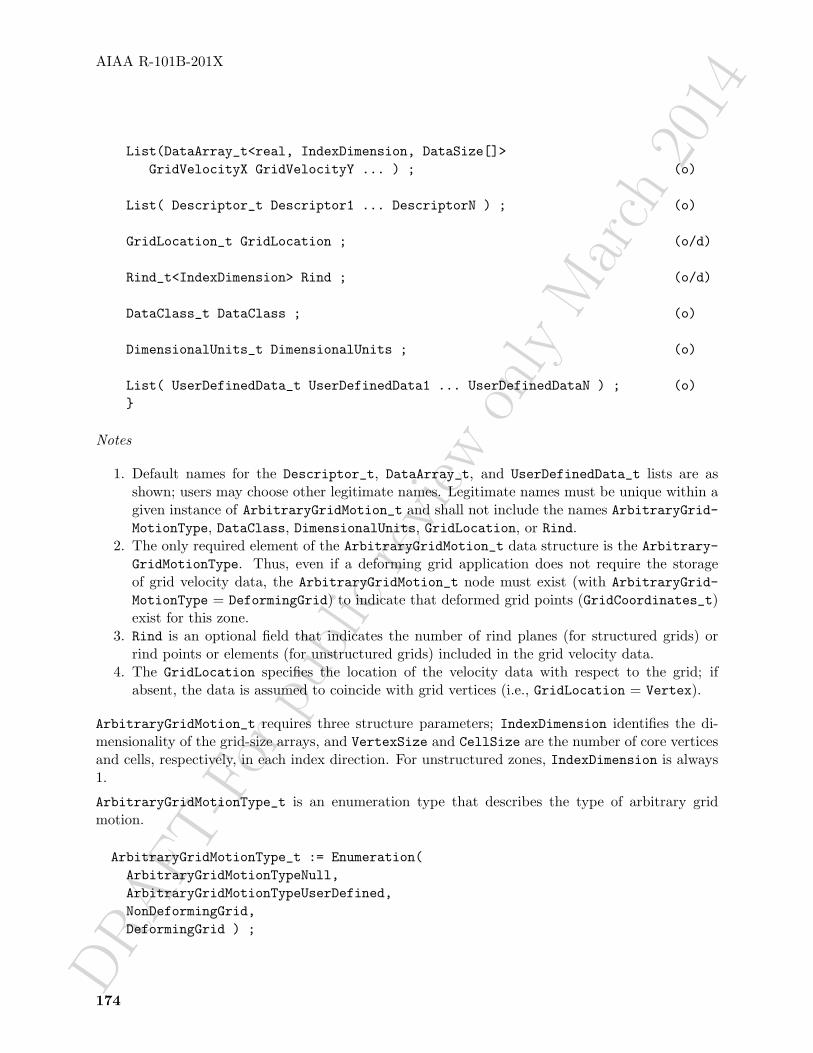
DRAFT

-For

publ

icre

view

only

Mar

ch20

14

AIAA R-101B-201X

List(DataArray_t<real, IndexDimension, DataSize[]>GridVelocityX GridVelocityY ... ) ; (o)







Notes

1. Default names for the Descriptor_t, DataArray_t, and UserDefinedData_t lists are asshown; users may choose other legitimate names. Legitimate names must be unique within agiven instance of ArbitraryGridMotion_t and shall not include the names ArbitraryGrid-MotionType, DataClass, DimensionalUnits, GridLocation, or Rind.

2. The only required element of the ArbitraryGridMotion_t data structure is the Arbitrary-GridMotionType. Thus, even if a deforming grid application does not require the storageof grid velocity data, the ArbitraryGridMotion_t node must exist (with ArbitraryGrid-MotionType = DeformingGrid) to indicate that deformed grid points (GridCoordinates_t)exist for this zone.

3. Rind is an optional field that indicates the number of rind planes (for structured grids) orrind points or elements (for unstructured grids) included in the grid velocity data.

4. The GridLocation specifies the location of the velocity data with respect to the grid; ifabsent, the data is assumed to coincide with grid vertices (i.e., GridLocation = Vertex).

ArbitraryGridMotion_t requires three structure parameters; IndexDimension identifies the di-mensionality of the grid-size arrays, and VertexSize and CellSize are the number of core verticesand cells, respectively, in each index direction. For unstructured zones, IndexDimension is always1.

ArbitraryGridMotionType_t is an enumeration type that describes the type of arbitrary gridmotion.

ArbitraryGridMotionType_t := Enumeration(ArbitraryGridMotionTypeNull,ArbitraryGridMotionTypeUserDefined,NonDeformingGrid,DeformingGrid ) ;

174

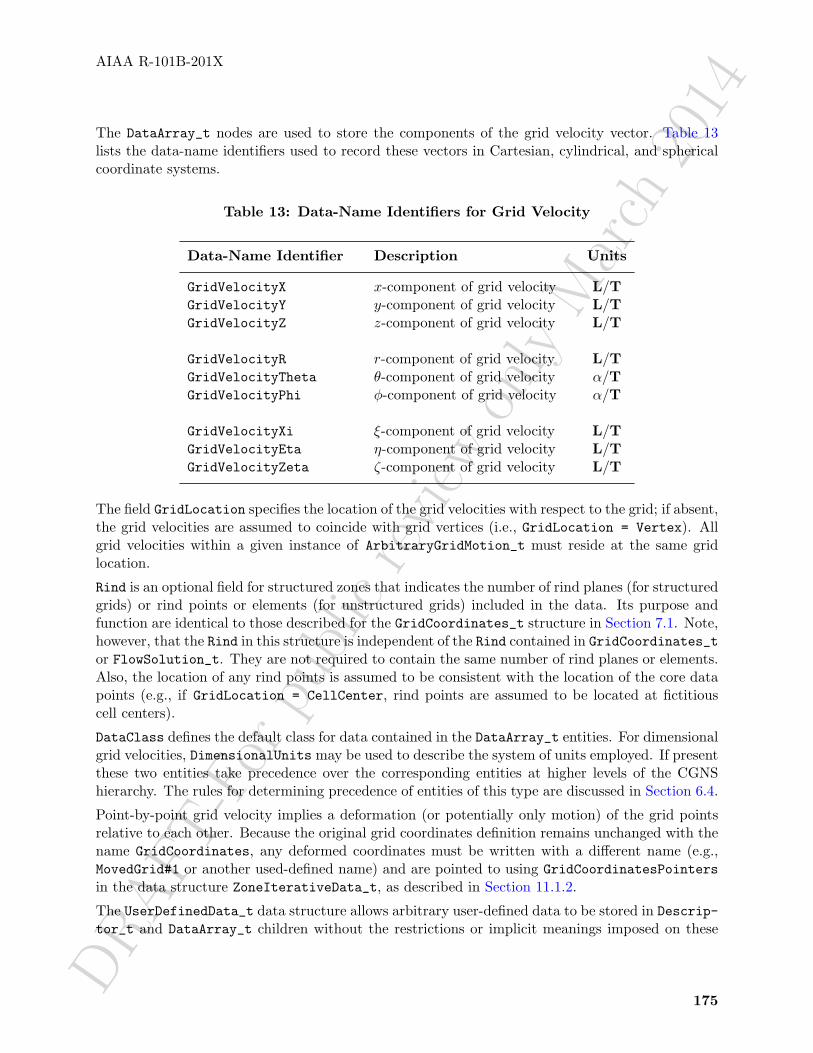
DRAFT

-For

publ

icre

view

only

Mar

ch20

14

AIAA R-101B-201X

The DataArray_t nodes are used to store the components of the grid velocity vector. Table 13lists the data-name identifiers used to record these vectors in Cartesian, cylindrical, and sphericalcoordinate systems.

Table 13: Data-Name Identifiers for Grid Velocity


GridVelocityX x-component of grid velocity L/TGridVelocityY y-component of grid velocity L/TGridVelocityZ z-component of grid velocity L/T

GridVelocityR r-component of grid velocity L/TGridVelocityTheta θ-component of grid velocity α/TGridVelocityPhi φ-component of grid velocity α/T

GridVelocityXi ξ-component of grid velocity L/TGridVelocityEta η-component of grid velocity L/TGridVelocityZeta ζ-component of grid velocity L/T

The field GridLocation specifies the location of the grid velocities with respect to the grid; if absent,the grid velocities are assumed to coincide with grid vertices (i.e., GridLocation = Vertex). Allgrid velocities within a given instance of ArbitraryGridMotion_t must reside at the same gridlocation.

Rind is an optional field for structured zones that indicates the number of rind planes (for structuredgrids) or rind points or elements (for unstructured grids) included in the data. Its purpose andfunction are identical to those described for the GridCoordinates_t structure in Section 7.1. Note,however, that the Rind in this structure is independent of the Rind contained in GridCoordinates_tor FlowSolution_t. They are not required to contain the same number of rind planes or elements.Also, the location of any rind points is assumed to be consistent with the location of the core datapoints (e.g., if GridLocation = CellCenter, rind points are assumed to be located at fictitiouscell centers).

DataClass defines the default class for data contained in the DataArray_t entities. For dimensionalgrid velocities, DimensionalUnits may be used to describe the system of units employed. If presentthese two entities take precedence over the corresponding entities at higher levels of the CGNShierarchy. The rules for determining precedence of entities of this type are discussed in Section 6.4.

Point-by-point grid velocity implies a deformation (or potentially only motion) of the grid pointsrelative to each other. Because the original grid coordinates definition remains unchanged with thename GridCoordinates, any deformed coordinates must be written with a different name (e.g.,MovedGrid#1 or another used-defined name) and are pointed to using GridCoordinatesPointersin the data structure ZoneIterativeData_t, as described in Section 11.1.2.

The UserDefinedData_t data structure allows arbitrary user-defined data to be stored in Descrip-tor_t and DataArray_t children without the restrictions or implicit meanings imposed on these

175

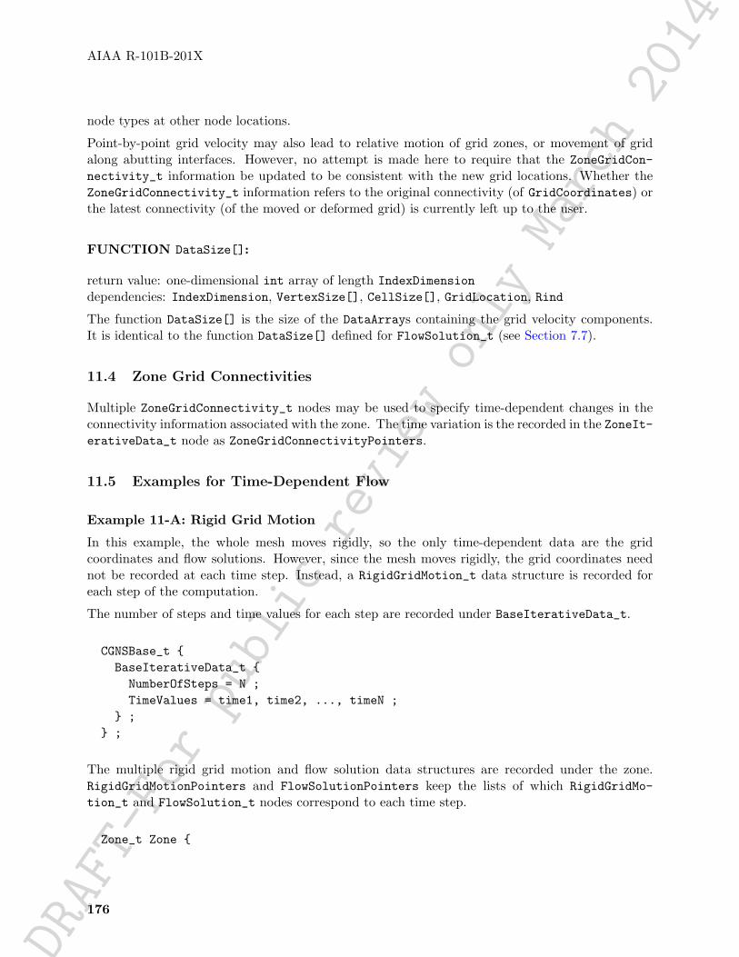
DRAFT-Forpublic

review

only


node types at other node locations.

Point-by-point grid velocity may also lead to relative motion of grid zones, or movement of gridalong abutting interfaces. However, no attempt is made here to require that the ZoneGridCon-nectivity_t information be updated to be consistent with the new grid locations. Whether theZoneGridConnectivity_t information refers to the original connectivity (of GridCoordinates) orthe latest connectivity (of the moved or deformed grid) is currently left up to the user.


return value: one-dimensional int array of length IndexDimensiondependencies: IndexDimension, VertexSize[], CellSize[], GridLocation, Rind

The function DataSize[] is the size of the DataArrays containing the grid velocity components.It is identical to the function DataSize[] defined for FlowSolution_t (see Section 7.7).

11.4 Zone Grid Connectivities

Multiple ZoneGridConnectivity_t nodes may be used to specify time-dependent changes in theconnectivity information associated with the zone. The time variation is the recorded in the ZoneIt-erativeData_t node as ZoneGridConnectivityPointers.

11.5 Examples for Time-Dependent Flow

Example 11-A: Rigid Grid Motion

In this example, the whole mesh moves rigidly, so the only time-dependent data are the gridcoordinates and flow solutions. However, since the mesh moves rigidly, the grid coordinates neednot be recorded at each time step. Instead, a RigidGridMotion_t data structure is recorded foreach step of the computation.

The number of steps and time values for each step are recorded under BaseIterativeData_t.

CGNSBase_t {BaseIterativeData_t {NumberOfSteps = N ;TimeValues = time1, time2, ..., timeN ;

} ;} ;

The multiple rigid grid motion and flow solution data structures are recorded under the zone.RigidGridMotionPointers and FlowSolutionPointers keep the lists of which RigidGridMo-tion_t and FlowSolution_t nodes correspond to each time step.

Zone_t Zone {

176

DRAFT-Forpublic

review

only


--- Time independent dataGridCoordinates_t GridCoordinatesZoneBC_t ZoneBCZoneGridConnectivity_t ZoneGridConnectivity

--- Time dependent dataRigidGridMotion_t RigidGridMotion#1RigidGridMotion_t RigidGridMotion#2...RigidGridMotion_t RigidGridmotion#N

FlowSolution_t Solution#0FlowSolution_t Solution#1FlowSolution_t Solution#2...FlowSolution_t Solution#N

ZoneIterativeData_t {RigidGridMotionPointers = {"RigidGridMotion#1", "RigidGridMotion#2", ...,

"RigidGridMotion#N"}FlowSolutionPointers = {"Solution#1", "Solution#2, ..., "Solution#N"}

}}

Note that there may be more solutions under a zone than those pointed to by FlowSolutionPoint-ers. In this example, Solution#0 could correspond to a restart solution.

Example 11-B: Deforming Grid Motion

In this example, velocity vectors are node dependent allowing for mesh deformation. In such acase, it is difficult or even impossible to recompute the mesh at each time step. Therefore the gridcoordinates are recorded for each step.

Multiple GridCoordinates_t and FlowSolution_t data structures are recorded under the zone.In addition, the data structure ArbitraryGridMotion_t is recorded for each step. GridCoordi-natesPointers, FlowSolutionPointers, and ArbitraryGridMotionPointers_t keep the list ofwhich grid coordinates definition, flow solution, and arbitrary grid motion definition correspond toeach time step.

Zone_t Zone {

--- Time independent dataZoneBC_t ZoneBCZoneGridConnectivity_t ZoneGridConnectivity

--- Time dependent dataList ( GridCoordinates_t GridCoordinates MovedGrid#1 MovedGrid#2 ...

177

DRAFT

-For

publ

icre

view

only

Mar

ch20

14

AIAA R-101B-201X

MovedGrid#N )List ( FlowSolution_t Solution#0 Solution#1 Solution#2 ... Solution#N )List ( ArbitraryGridMotion_t ArbitraryGridMotion#1

ArbitraryGridMotion#2 ... ArbitraryGridMotion#N )ZoneIterativeData_t {GridCoordinatesPointers = {"MovedGrid#1", "MovedGrid#2", ...,

"MovedGrid#N"}FlowSolutionPointers = {"Solution#1", "Solution#2, ..., "Solution#N"}ArbitraryGridMotionPointers = {"ArbitraryGridMotion#1",

"ArbitraryGridMotion#2", ..., "ArbitraryGridMotion#N"}}

}

178

DRAFT-Forpublic

review

only


Example 11-C: Adapted Unstructured Mesh

In this example, the mesh size varies at each remeshing, therefore new zones must be created.ZonePointers is used to keep a record of the zone definition corresponding to each recorded step.Let’s assume that the solution is recorded every 50 iterations, and the grid is adapted every 100iterations.

The number of steps, iteration values for each step, number of zones for each step, and name ofthese zones are recorded under BaseIterativeData_t.

CGNSBase_t {BaseIterativeData_t {NumberOfSteps = 4IterationValues = {50, 100, 150, 200}NumberOfZones = {1, 1, 1, 1}ZonePointers = {"Zone1", "Zone1", "Zone2", "Zone2"}

}}

Each zone holds 2 solutions recorded at 50 iterations apart. Therefore the ZoneIterativeData_tdata structure must be included to keep track of the FlowSolutionPointers.

Zone_t Zone1 {

--- Constant dataGridCoordinates_t GridCoordinatesElements_t ElementsZoneBC_t ZoneBC

--- Variable dataList ( FlowSolution_t InitialSolution Solution50 Solution100 )ZoneIterativeData_t {FlowSolutionPointers = {"Solution50", "Solution100", "Null", "Null"}

}}

Zone_t Zone2 {

--- Constant dataGridCoordinates_t GridCoordinatesElements_t ElementsZoneBC_t ZoneBC

--- Variable dataList ( FlowSolution_t RestartSolution Solution150 Solution200 )ZoneIterativeData_t {

179

DRAFT-Forpublic

review

only


FlowSolutionPointers = {"Null", "Null", "Solution150", "Solution200"}}

}

Notes

1. If the solution was recorded every 100 iterations instead of every 50 iterations, then each zonewould have only one FlowSolution_t node and the data structure ZoneIterativeData_twould not be required.

2. Note that FlowSolutionPointers is always an array of size NumberOfSteps even if some ofthe steps are defined in another zone.

Example 11-D: Combination of Grid Motion and Time-Accuracy

The following is an example demonstrating the use of the rigid grid motion, arbitrary grid motion,and time-accurate data nodes in CGNS. The example is a 3-zone case. Zone 1 is rigidly rotatingabout the x-axis at a constant rate, with no translation. Zone 2 is a deforming zone. Zone 3 isa fixed zone. This is a time-accurate simulation with two solutions saved at times 15.5 and 31.0,corresponding to iteration numbers 1000 and 2000.

No units are given in this example, but a real case would establish them. Also, a real case wouldinclude connectivity, boundary conditions, and possibly other information as well. Each indentationrepresents a level down (a child) from the parent node.

Base (CGNSBase_t)SimulationType (SimulationType_t) Data=TimeAccurateBaseIterativeData (BaseIterativeData_t) Data=NumberOfSteps=2TimeValues (DataArray_t) Data=(15.5, 31.0)IterationValues (DataArray_t) Data=(1000, 2000)

Zone#1 (Zone_t)GridCoordinates (GridCoordinates_t)CoordinateX (DataArray_t)CoordinateY (DataArray_t)

RigidGridMotion#1(RigidGridMotion_t) Data=RigidGridMotionType=ConstantRateOriginLocation (DataArray_t) Data=(0,0,0), (0,0,0)RigidRotationAngle (DataArray_t) Data=(5., 0., 0.)

RigidGridMotion#2(RigidGridMotion_t) Data=RigidGridMotionType=ConstantRateOriginLocation (DataArray_t) Data=(0,0,0), (0,0,0)RigidRotationAngle (DataArray_t) Data=(10., 0., 0.)

ZoneIterativeData (ZoneIterativeData_t)RigidGridMotionPointers (DataArray_t) Data=(RigidGridMotion#1,

RigidGridMotion#2)FlowSolutionPointers (DataArray_t) Data=(Soln#1, Soln#2)

Soln#1 (FlowSolution_t)Density (DataArray_t)VelocityX (DataArray_t)

180

DRAFT

-For

publ

icre

view

only

Mar

ch20

14

AIAA R-101B-201X



MovedGrid#1 (GridCoordinates_t)CoordinateX (DataArray_t)CoordinateY (DataArray_t)

MovedGrid#2 (GridCoordinates_t)CoordinateX (DataArray_t)CoordinateY (DataArray_t)

ArbitraryGridMotion#1 (ArbitraryGridMotion_t)Data=ArbitraryGridMotionType=DeformingGrid

ArbitraryGridMotion#2 (ArbitraryGridMotion_t)Data=ArbitraryGridMotionType=DeformingGrid

GridVelocityX (DataArray_t)GridVelocityY (DataArray_t)

ZoneIterativeData (ZoneIterativeData_t)ArbitraryGridMotionPointers (DataArray_t) Data=("ArbitraryGridMotion#1",

"ArbitraryGridMotion#2")GridCoordinatesPointers (DataArray_t) Data=("MovedGrid#1",

"MovedGrid#2")FlowSolutionPointers (DataArray_t) Data=("Soln#1", "Soln#2")




ZoneIterativeData (ZoneIterativeData_t)FlowSolutionPointers (DataArray_t) Data=("Soln#1", "Soln#2")



181

DRAFT

-For

publ

icre

view

only

Mar

ch20

14

AIAA R-101B-201X

Notes

1. Under BaseIterativeData_t, one can give either TimeValues, or IterationValues, or both.In the example, both have been given.

2. The nodes NumberOfZones and ZonePointers are not required under the BaseIterative-Data_t node in this example because all existing zones are used for each time step.

3. Under ArbitraryGridMotion, the GridVelocity data is optional. In the example, it wasput under one of the nodes but not under the other. Hence, "ArbitraryGridMotion#1" inthe example has no children nodes, while "ArbitraryGridMotion#2" does.

4. The pointers under ZoneIterativeData_t point to names of nodes within the same zone.Thus, for example, Soln#1 refers to the flow solution named Soln#1 in the same zone, eventhough there are flow solution nodes in other zones with the same name.

5. The name GridCoordinates always refers to the original grid. Thus, when a grid is de-forming, the deformed values must be put in GridCoordinates_t nodes of a different name.In the example, the deformed grids (for Zone#2) at the two times of interest were put into"MovedGrid#1" and "MovedGrid#2".

6. Because the node "ArbitraryGridMotion#1" doesn’t really add any information in the cur-rent example (since it was decided not to store GridVelocity data under it), one has theoption of not including this node in the CGNS file. If it is removed, then under Zone#2’sZoneIterativeData, the ArbitraryGridMotionPointers data would be replaced by:

Data = (Null, ArbitraryGridMotion#2)

182

DRAFT

-For

publ

icre

view

only

Mar

ch20

14

AIAA R-101B-201X

12 Miscellaneous Data Structures

This section contains miscellaneous structure types for describing reference states, convergencehistory, discrete field data, integral or global data, families, and user-defined data.

12.1 Reference State Structure Definition: ReferenceState_t

ReferenceState_t describes a reference state, which is a list of geometric or flow-state quantitiesdefined at a common location or condition. Examples of typical reference states associated withCFD calculations are freestream, plenum, stagnation, inlet and exit. Note that providing a Ref-erenceState description is particularly important if items elsewhere in the CGNS database areNormalizedByUnknownDimensional.

ReferenceState_t :={Descriptor_t ReferenceStateDescription ; (o)List( Descriptor_t Descriptor1 ... DescriptorN ) ; (o)





Notes

1. Default names for the Descriptor_t, DataArray_t, and UserDefinedData_t lists are asshown; users may choose other legitimate names. Legitimate names must be unique withina given instance of ReferenceState_t and shall not include the names DataClass, Dimen-sionalUnits, or ReferenceStateDescription.

Data-name identifiers associated with ReferenceState are shown in Table 14.

In addition, any flowfield quantities (such as Density, Pressure, etc.) can be included in theReferenceState.

The reference length L (LengthReference) may be necessary for NormalizedByUnknownDimen-sional databases, to define the length scale used for nondimensionalizations. It may be the sameor different from the Reynolds_Length used to define the Reynolds number.

Because of different definitions for angle of attack and angle of yaw, these quantities are not ex-plicitly defined in the SIDS. Instead, the user can unambigouosly denote the freestream velocity

183

DRAFT-Forpublic

review

only


Table 14: Data-Name Identifiers for Reference State


Mach Mach number, M = q/c -Mach_Velocity Velocity scale, q L/TMach_VelocitySound Speed of sound scale, c L/TReynolds Reynolds number, Re = V LR/ν -Reynolds_Velocity Velocity scale, V L/TReynolds_Length Length scale, LR LReynolds_ViscosityKinematic Kinematic viscosity scale, ν L2/TLengthReference Reference length, L L

vector direction by giving VelocityX, VelocityY, and VelocityZ in ReferenceState, (with thereference state denoting the freestream).

Care should be taken when defining the reference state quantities to ensure consistency. (See thediscussion in Section 5.2.3.) For example, if velocity, length, and time are all defined, then thevelocity stored should be length/time. If consistency is not followed, different applications couldinterpret the resulting data in different ways.

DataClass defines the default for the class of data contained in the reference state. If any referencestate quantities are dimensional, DimensionalUnits may be used to describe the system of dimen-sional units employed. If present, these two entities take precedence over all corresponding entitiesat higher levels of the hierarchy. These precedence rules are further discussed in Section 6.4.


We recommend using the ReferenceStateDescription entity to document the flow conditions.The format of the documentation is currently unregulated.

12.2 Reference State Example

An example is presented in this section of a reference state entity that contains dimensional data.An additional example of a nondimensional reference state is provided in Appendix B.

Example 12-A: Reference State with Dimensional Data

A freestream reference state where all data quantities are dimensional. Standard atmosphericconditions at sea level are assumed for static quantities, and all stagnation variables are obtainedusing the isentropic relations. The flow velocity is 200 m/s aligned with the x-axis. Dimensionalunits of kilograms, meters, and seconds are used. The data class and system of units are specifiedat the ReferenceState_t level rather than attaching this information directly to the DataArray_tentities for each reference quantity. Data-name identifiers are provided in Appendix A.

184

DRAFT

-For

publ

icre

view

only

Mar

ch20

14

AIAA R-101B-201X

ReferenceState_t ReferenceState ={{Descriptor_t ReferenceStateDescription ={{Data(char, 1, 45) = "Freestream at standard atmospheric conditions" ;}} ;


DimensionalUnits_t DimensionalUnits ={{MassUnits = Kilogram ;LengthUnits = Meter ;TimeUnits = Second ;TemperatureUnits = Kelvin ;AngleUnits = Radian ;}} ;

DataArray_t<real, 1, 1> VelocityX ={{Data(real, 1, 1) = 200. ;}} ;

DataArray_t<real, 1, 1> VelocityY = {{ 0. }} ;DataArray_t<real, 1, 1> VelocityZ = {{ 0. }} ;

DataArray_t<real, 1, 1> Pressure = {{ 1.0132E+05 }} ;DataArray_t<real, 1, 1> Density = {{ 1.226 }} ;DataArray_t<real, 1, 1> Temperature = {{ 288.15 }} ;DataArray_t<real, 1, 1> VelocitySound = {{ 340. }} ;DataArray_t<real, 1, 1> ViscosityMolecular = {{ 1.780E-05 }} ;

DataArray_t<real, 1, 1> PressureStagnation = {{ 1.2806E+05 }} ;DataArray_t<real, 1, 1> DensityStagnation = {{ 1.449 }} ;DataArray_t<real, 1, 1> TemperatureStagnation = {{ 308.09 }} ;DataArray_t<real, 1, 1> VelocitySoundStagnation = {{ 351.6 }} ;

DataArray_t<real, 1, 1> PressureDynamic = {{ 0.2542E+05 }} ;}} ;

Note that all DataArray_t entities except VelocityX have been abbreviated.

12.3 Convergence History Structure Definition: ConvergenceHistory_t

Flow solver convergence history information is described by the ConvergenceHistory_t structure.This structure contains the number of iterations and a list of data arrays containing convergence

185

DRAFT

-For

publ

icre

view

only

Mar

ch20

14

AIAA R-101B-201X

information at each iteration.

ConvergenceHistory_t :={Descriptor_t NormDefinitions ; (o)List( Descriptor_t Descriptor1 ... DescriptorN ) ; (o)

int Iterations ; (r)

List( DataArray_t<DataType, 1, Iterations>DataArray1 ... DataArrayN ) ; (o)




Notes

1. Default names for the Descriptor_t, DataArray_t, and UserDefinedData_t lists are asshown; users may choose other legitimate names. Legitimate names must be unique withina given instance of ConvergenceHistory_t and shall not include the names DataClass,DimensionalUnits, or NormDefinitions.

2. Iterations is the only required field for ConvergenceHistory_t.

Iterations identifies the number of iterations for which convergence information is recorded. Thisvalue is also passed into each of the DataArray_t entities, defining the length of the data arrays.

DataClass defines the default for the class of data contained in the convergence history. If anyconvergence-history data is dimensional, DimensionalUnits may be used to describe the system ofdimensional units employed. If present, these two entities take precedence over all correspondingentities at higher levels of the hierarchy. These precedence rules are further discussed in Section 6.4.


Measures used to record convergence vary greatly among current flow-solver implementations. Con-vergence information typically includes global forces, norms of equation residuals, and norms of so-lution changes. Attempts to systematically define a set of convergence measures within the CGNSproject have been futile. For global parameters, such as forces and moments, Appendix A lists aset of standardized data-array identifiers. For equations residuals and solution changes, no suchstandard list exists. It is suggested that data-array identifiers for norms of equations residualsbegin with RSD, and those for solution changes begin with CHG. For example, RSDMassRMS could beused for the L2-norm (RMS) of mass conservation residuals. It is also strongly recommended that

186

DRAFT

-For

publ

icre

view

only

Mar

ch20

14

AIAA R-101B-201X

NormDefinitions be utilized to describe the convergence information recorded in the data arrays.The format used to describe the convergence norms in NormDefinitions is currently unregulated.

12.4 Discrete Data Structure Definition: DiscreteData_t

DiscreteData_t provides a description of generic discrete data (i.e., data defined on a computa-tional grid); it is identical to FlowSolution_t except for its type name. This structure can be usedto store field data, such as fluxes or equation residuals, that is not typically considered part of theflow solution. DiscreteData_t contains a list for data arrays, identification of grid location, and amechanism for identifying rind-point data included in the data arrays. All data contained withinthis structure must be defined at the same grid location and have the same amount of rind-pointdata.

DiscreteData_t< int CellDimension, int IndexDimension,int VertexSize[IndexDimension],int CellSize[IndexDimension] > :=




IndexRange_t<IndexDimension> PointRange ; (o)IndexArray_t<IndexDimension, ListLength[], int> PointList ; (o)

List( DataArray_t<DataType, IndexDimension, DataSize[]>DataArray1 ... DataArrayN ) ; (o)




Notes

1. Default names for the Descriptor_t, DataArray_t, and UserDefinedData_t lists are asshown; users may choose other legitimate names. Legitimate names must be unique within agiven instance of DiscreteData_t and shall not include the names DataClass, Dimension-alUnits, GridLocation, PointRange, PointList, or Rind.

2. There are no required fields for DiscreteData_t. GridLocation has a default of Vertex ifabsent. Rind also has a default if absent; the default is equivalent to having an instance ofRind whose RindPlanes array contains all zeros (see Section 4.8).

187

DRAFT

-For

publ

icre

view

only

Mar

ch20

14

AIAA R-101B-201X

3. Both of the fields PointRange and PointList are optional. Only one of these two fields maybe specified.

4. The structure parameter DataType must be consistent with the data stored in the DataAr-ray_t entities (see Section 5.1).

5. For unstructured zones GridLocation options are limited to Vertex or CellCenter, unlessone of PointRange or PointList is present.

6. Indexing of data within the DataArray_t structures, must be consistent with the associatednumbering of vertices or elements.

DiscreteData_t requires four structure parameters: CellDimension identifies the dimensionalityof cells or elements, IndexDimension identifies the dimensionality of the grid size arrays, andVertexSize and CellSize are the number of core vertices and cells, respectively, in each indexdirection. For unstructured zones, IndexDimension is always 1.

The arrays of discrete data are stored in the list of DataArray_t entities. The field GridLocationspecifies the location of the data with respect to the grid; if absent, the data is assumed tocoincide with grid vertices (i.e., GridLocation = Vertex). All data within a given instance ofDiscreteData_t must reside at the same grid location.

For structured grids, the value of GridLocation alone specifies the location and indexing of thediscrete data. Vertices are explicity indexed. Cell centers and face centers are indexed using theminimum of the connecting vertex indices, as described in the section Structured Grid Notationand Indexing Conventions (Section 3.2).

For unstructured grids, the value of GridLocation alone specifies location and indexing of discretedata only for vertex and cell-centered data. The reason for this is that element-based grid connec-tivity provided in the Elements_t data structures explicitly indexes only vertices and cells. Fordata stored at alternate grid locations (e.g. edges), additional connectivity information is needed.This is provided by the optional fields PointRange and PointList; these refer to vertices, edges,faces or cell centers, depending on the values of CellDimension and GridLocation. The followingtable shows these relations.




Although intended for edge or face-based discrete data for unstructured grids, the fields PointRange/Listmay also be used to (redundantly) index vertex and cell-centered data. In all cases, indexing ofdiscrete data corresponds to the element numbering as defined in the Elements_t data structures.

Rind is an optional field that indicates the number of rind planes (for structured grids) or rind pointsor elements (for unstructured grids) included in the data. Its purpose and function are identical tothose described in Section 7.1. Note, however, that the Rind in this structure is independent of the

188

DRAFT-Forpublic

review

only


Rind contained in GridCoordinates_t. They are not required to contain the same number of rindplanes or elements. Also, the location of any flow-solution rind points is assumed to be consistentwith the location of the core flow solution points (e.g., if GridLocation = CellCenter, rind pointsare assumed to be located at fictitious cell centers).

DataClass defines the default class for data contained in the DataArray_t entities. For dimensionaldata, DimensionalUnits may be used to describe the system of units employed. If present thesetwo entities take precedence over the corresponding entities at higher levels of the CGNS hierarchy.The rules for determining precedence of entities of this type are discussed in Section 6.4.




DiscreteData_t requires the structure function ListLength, which is used to specify the numberof entities (e.g. vertices) corresponding to a given PointRange or PointList. If PointRange isspecified, then ListLength is obtained from the number of points (inclusive) between the beginningand ending indices of PointRange. If PointList is specified, then ListLength is the number ofindices in the list of points. In this situation, ListLength becomes a user input along with theindices of the list PointList. By “user” we mean the application code that is generating the CGNSdatabase.


return value: one-dimensional int array of length IndexDimensiondependencies: IndexDimension, VertexSize[], CellSize[], GridLocation, Rind, ListLength

The function DataSize[] is the size of discrete-data arrays. It is identical to the function Data-Size[] defined for FlowSolution_t (see Section 7.7).

12.5 Integral Data Structure Definition: IntegralData_t

IntegralData_t provides a description of generic global or integral data that may be associatedwith a particular zone or an entire database. In contrast to DiscreteData_t, integral data is notassociated with any specific field location.

IntegralData_t :={List( Descriptor_t Descriptor1 ... DescriptorN ) ; (o)


189

DRAFT-Forpublic

review

only





Notes

1. Default names for the Descriptor_t, DataArray_t, and UserDefinedData_t lists are asshown; users may choose other legitimate names. Legitimate names must be unique withina given instance of DiscreteData_t and shall not include the names DataClass or Dimen-sionalUnits.

2. There are no required fields for IntegralData_t.3. The structure parameter DataType must be consistent with the data stored in the DataAr-

ray_t entities (see Section 5.1).

DataClass defines the default class for data contained in the DataArray_t entities. For dimensionaldata, DimensionalUnits may be used to describe the system of units employed. If present thesetwo entities take precedence over the corresponding entities at higher levels of the CGNS hierarchy.The rules for determining precedence of entities of this type are discussed in Section 6.4.


12.6 Family Data Structure Definition: Family_t

Geometric associations need to be set through one layer of indirection. That is, rather than settingthe geometry data for each mesh entity (nodes, edges, and faces), they are associated to intermediateobjects. The intermediate objects are in turn linked to nodal regions of the computational mesh.We define a CFD family as this intermediate object. This layer of indirection is necessary sincethere is rarely a 1-to-1 connection between mesh regions and geometric entities.

The Family_t data structure holds the CFD family data. Each mesh surface is linked to thegeometric entities of the CAD databases by a name attribute. This attribute corresponds to afamily of CAD geometric entities on which the mesh face is projected. Each one of these geometricentities is described in a CAD file and is not redefined within the CGNS file. A Family_t datastructure may be included in the CGNSBase_t structure for each CFD family of the model.

The Family_t structure contains all information pertinent to a CFD family. This informationincludes the name attribute or family name, the boundary conditions applicable to these meshregions, and the referencing to the CAD databases.

Family_t :=

190

DRAFT

-For

publ

icre

view

only

Mar

ch20

14

AIAA R-101B-201X


FamilyBC_t FamilyBC ; (o)

List( GeometryReference_t GeometryReference1 ... GeometryReferenceN ) ; (o)


List( FamilyName_t FamilyName1 ... FamilyNameN ) ; (o)



Notes

1. All data structures contained in Family_t are optional.2. Default names for the Descriptor_t, GeometryReference_t, and UserDefinedData_t lists

are as shown; users may choose other legitimate names. Legitimate names must be unique atthis level and must not include the names FamilyBC, Ordinal, or RotatingCoordinates.

3. The CAD referencing data are written in the GeometryReference_t data structures. Theyidentify the CAD systems and databases where the geometric definition of the family is stored.

4. The boundary condition type pertaining to a family is contained in the data structure Fam-ilyBC_t. If this boundary condition type is to be used, the BCType specified under BC_t mustbe FamilySpecified.

5. For the purpose of defining zone properties, families are extended to a volume of cells. Insuch case, the GeometryReference_t structures are not used.

6. The mesh is linked to the family by attributing a family name to a BC patch or a zone in thedata structure BC_t or Zone_t, respectively.

7. A hierarchy of families is possible through the list of <tt>FamilyName t</tt> nodes. Thesenodes contain both a user defined node name and a family name. The node name<tt>FamilyParent</tt>may be used to specify the family name for the parent of the current <tt>Family t</tt>node.

8. Ordinal is defined in the SIDS as a user-defined integer with no restrictions on the valuesthat it can contain. It may be used here to attribute a number to the family.

Rotation of the CFD family may be defined using the RotatingCoordinates_t data structure.


191

DRAFT

-For

publ

icre

view

only

Mar

ch20

14

AIAA R-101B-201X

12.7 Geometry Reference Structure Definition: GeometryReference_t

The standard interface data structure identifies the CAD systems used to generate the geometry, theCAD files where the geometry is stored, and the geometric entities corresponding to the family. TheGeometryReference_t structures contain all the information necessary to associate a CFD familyto the CAD databases. For each GeometryReference_t structure, the CAD format is recorded inGeometryFormat, and the CAD file in GeometryFile. The geometry entity or entities within thisCAD file that correspond to the family are recorded under the GeometryEntity_t nodes.

GeometryReference_t :={List( Descriptor_t Descriptor1 ... DescriptorN ) ; (o)

GeometryFormat_t GeometryFormat ; (r)

GeometryFile_t GeometryFile ; (r)

List (GeometryEntity_t GeometryEntity1 ... GeometryEntityN) ; (o/d)


The GeometryFormat is an enumeration type that identifies the CAD system used to generate thegeometry.

GeometryFormat_t := Enumeration(GeometryFormatNull,GeometryFormatUserDefined,NASA-IGES,SDRC,Unigraphics,ProEngineer,ICEM-CFD ) ;

Notes

1. Default names for the Descriptor_t, GeometryEntity_t, and UserDefinedData_t lists areas shown; users may choose other legitimate names. Legitimate names must be unique at thislevel and must not include the names GeometryFile or GeometryFormat.

2. By default, there is only one GeometryEntity and its name is the family name.3. There is no limit to the number of CAD files or CAD systems referenced in a CGNS file.

Different parts of the same model may be described with different CAD files of different CADsystems.

4. Other CAD geometry formats may be added to this list as needed.

192

DRAFT

-For

publ

icre

view

only

Mar

ch20

14

AIAA R-101B-201X

12.8 Family Boundary Condition Structure Definition: FamilyBC_t

One of the main advantages of the concept of a layer of indirection (called a family here) is that themesh density and the geometric entities may be modified without altering the association betweennodes and intermediate objects, or between intermediate objects and geometric entities. Thisis very beneficial when handling boundary conditions and properties. Instead of setting boundaryconditions directly on mesh entities, or on CAD entities, they may be associated to the intermediateobjects. Since these intermediate objects are stable in the sense that they are not subject to meshor geometric variations, the boundary conditions do not need to be redefined each time the modelis modified. Using the concept of indirection, the boundary conditions and property settings aremade independent of operations such as geometric changes, modification of mesh topology (i.e.,splitting into zones), mesh refinement and coarsening, etc.

The FamilyBC_t data structure contains the boundary condition type. It is envisioned that it willbe extended to hold both material and volume properties as well.

FamilyBC_t :={BCType_t BCType; (r)

List( FamilyBCDataSet_t<ListLength>; BCDataSet1 ... BCDataSetN ) ; (o)} ;

Notes

1. Default names for the FamilyBCDataSet_t list are as shown; users may choose other legitimatenames. Legitimate names must be unique within a given instance of FamilyBC_t and shallnot include the name BCType.

BCType specifies the boundary-condition type, which gives general information on the boundary-condition equations to be enforced. Boundary conditions are to be applied at the locations specifiedby the BC_t structure(s) associated with the CFD family.

The FamilyBC_t structure provides for a list of boundary-condition data sets. In general, theproper FamilyBCDataSet_t instance to impose on the CFD family is determined by the BCTypeassociation table (Table 4 on p. 133). The mechanics of determining the proper data set to imposeis described in Section 9.8.

For a few boundary conditions, such as a symmetry plane or polar singularity, the value of BCTypecompletely describes the equations to impose, and no instances of FamilyBCDataSet_t are needed.For“simple”boundary conditions, where a single set of Dirichlet and/or Neumann data is applied, asingle FamilyBCDataSet_t will likely appear (although this is not a requirement). For “compound”boundary conditions, where the equations to impose are dependent on local flow conditions, severalinstances of FamilyBCDataSet_t will likely appear; the procedure for choosing the proper data setis more complex as described in Section 9.8.

193

DRAFT

-For

publ

icre

view

only

Mar

ch20

14

AIAA R-101B-201X

12.9 Family Boundary Condition Data Set Structure Definition: FamilyBC-

DataSet_t

FamilyBCDataSet_t contains Dirichlet and Neumann data for a single set of boundary-conditionequations. Its intended use is for simple boundary-condition types, where the equations imposeddo not depend on local flow conditions.

FamilyBCDataSet_t :={List( Descriptor_t Descriptor1 ... DescriptorN ) ; (o)

BCTypeSimple_t BCTypeSimple ; (r)

BCData_t<1> DirichletData ; (o)BCData_t<1> NeumannData ; (o)





Notes

1. Default names for the Descriptor_t and UserDefinedData_t lists are as shown; users maychoose other legitimate names. Legitimate names must be unique within a given instanceof FamilyBCDataSet_t and shall not include the names BCTypeSimple, DataClass, Dimen-sionalUnits, DirichletData, NeumannData or ReferenceState.

2. BCTypeSimple is the only required field. All other fields are optional and the Descriptor_tlist may be empty.

BCTypeSimple specifies the boundary-condition type, which gives general information on the bound-ary-condition equations to be enforced. BCTypeSimple_t is defined in Section 9.7 along with themeanings of all the BCTypeSimple values. BCTypeSimple is also used for matching boundarycondition data sets as discussed in Section 9.8.

Boundary-condition data is separated by equation type into Dirichlet and Neumann conditions.Dirichlet boundary conditions impose the value of the given variables, whereas Neumann boundaryconditions impose the normal derivative of the given variables. The mechanics of specifying Dirichletand Neumann data for boundary conditions is covered in Section 9.9.

The substructures DirichletData and NeumannData contain boundary-condition data defined asglobally constant over the family.

194

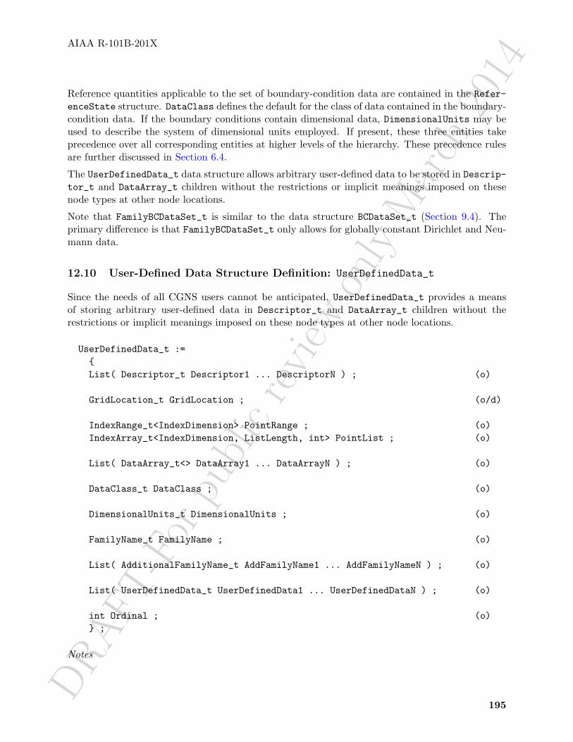
DRAFT

-For

publ

icre

view

only

Mar

ch20

14

AIAA R-101B-201X

Reference quantities applicable to the set of boundary-condition data are contained in the Refer-enceState structure. DataClass defines the default for the class of data contained in the boundary-condition data. If the boundary conditions contain dimensional data, DimensionalUnits may beused to describe the system of dimensional units employed. If present, these three entities takeprecedence over all corresponding entities at higher levels of the hierarchy. These precedence rulesare further discussed in Section 6.4.


Note that FamilyBCDataSet_t is similar to the data structure BCDataSet_t (Section 9.4). Theprimary difference is that FamilyBCDataSet_t only allows for globally constant Dirichlet and Neu-mann data.

12.10 User-Defined Data Structure Definition: UserDefinedData_t

Since the needs of all CGNS users cannot be anticipated, UserDefinedData_t provides a meansof storing arbitrary user-defined data in Descriptor_t and DataArray_t children without therestrictions or implicit meanings imposed on these node types at other node locations.

UserDefinedData_t :={List( Descriptor_t Descriptor1 ... DescriptorN ) ; (o)


IndexRange_t<IndexDimension> PointRange ; (o)IndexArray_t<IndexDimension, ListLength, int> PointList ; (o)








Notes

195

DRAFT

-For

publ

icre

view

only

Mar

ch20

14

AIAA R-101B-201X

1. Default names for the Descriptor_t, DataArray_t, and UserDefinedData_t lists are asshown; users may choose other legitimate names. Legitimate names must be unique withina given instance of UserDefinedData_t and shall not include the names DataClass, Dimen-sionalUnits, FamilyName, GridLocation, Ordinal, PointList, or PointRange.

2. GridLocation may be set to Vertex, IFaceCenter, JFaceCenter, KFaceCenter, FaceCen-ter, CellCenter, or EdgeCenter. If GridLocation is absent, then its default value is Vertex.When GridLocation is set to Vertex, then PointList or PointRange refer to node indices,for both structured and unstructured grids. When GridLocation is set to FaceCenter, thenPointList or PointRange refer to face elements.

3. GridLocation, PointRange, and PointList may only be used when UserDefinedData_t islocated below a Zone_t structure in the database hierarchy.

4. Only one of PointRange and PointList may be specified.

12.11 Gravity Data Structure Definition: Gravity_t

The Gravity_t data structure may be used to define the gravitational vector.

Gravity_t :={List( Descriptor_t Descriptor1 ... DescriptorN ) ; (o)

DataArray_t<real, 1, PhysicalDimension> GravityVector ; (r)




Notes

1. Default names for the Descriptor_t and UserDefinedData_t lists are as shown; users maychoose other legitimate names. Legitimate names must be unique within a given instance ofGravity_t and shall not include the names DataClass, DimensionalUnits, or GravityVec-tor.

The only required field under the Gravity_t data structure is GravityVector, which contains thecomponents of the gravity vector in the coordinate system being used.

DataClass defines the default class for data contained in the DataArray_t entity. For dimensionaldata, DimensionalUnits may be used to describe the system of units employed. If present, thesetwo entities take precedence over the corresponding entities at higher levels of the CGNS hierarchy,following the standard precedence rules.

196

DRAFT

-For

publ

icre

view

only

Mar

ch20

14

AIAA R-101B-201X


197

DRAFT

-For

publ

icre

view

only

Mar

ch20

14

DRAFT

-For

publ

icre

view

only

Mar

ch20

14

AIAA R-101B-201X

A Conventions for Data-Name Identifiers

Identifiers or names can be attached to DataArray_t entities to identify and describe the quantitybeing stored. To facilitate communication between different application codes, we propose to estab-lish a set of standardized data-name identifiers with fairly precise definitions. For any identifier inthis set, the associated data should be unambiguously understood. In essence, this section proposesstandardized terminology for labeling CFD-related data, including grid coordinates, flow solution,turbulence model quantities, nondimensional governing parameters, boundary condition quantities,and forces and moments.

We use the convention that all standardized identifiers denote scalar quantities; this is consistentwith the intended use of the DataArray_t structure type to describe an array of scalars. Forquantities that are vectors, such as velocity, their components are listed.

Included with the lists of standard data-name identifiers are the fundamental units of dimensions as-sociated with that quantity. The following notation is used for the fundamental units: M is mass, Lis length, T is time, Θ is temperature, α is angle, and I is electric current. These fundamental unitsare directly associated with the elements of the DimensionalExponents_t structure. For example,a quantity that has dimensions ML/T corresponds to MassExponent = +1, LengthExponent =+1, and TimeExponent = -1.

Unless otherwise noted, all quantities in the following sections denote floating-point data types,and the appropriate DataType structure parameter for DataArray_t is real.

A.1 Coordinate Systems

Coordinate systems for identifying physical location are as follows:

System 3-D 2-D

Cartesian (x, y, z) (x, y) or (x, z) or (y, z)Cylindrical (r, θ, z) (r, θ)Spherical (r, θ, φ)Auxiliary (ξ, η, ζ) (ξ, η) or (ξ, ζ) or (η, ζ)

Associated with these coordinate systems are the following unit vector conventions:

x-direction ex r-direction er ξ-direction eξy-direction ey θ-direction eθ η-direction eηz-direction ez φ-direction eφ ζ-direction eζ

Note that er, eθ and eφ are functions of position.

We envision that one of the “standard” coordinate systems (Cartesian, cylindrical or spherical) willbe used within a zone (or perhaps the entire database) to define grid coordinates and other relateddata. The auxiliary coordinates will be used for special quantities, including forces and moments,which may not be defined in the same coordinate system as the rest of the data. When auxiliary

199

DRAFT

-For

publ

icre

view

only

Mar

ch20

14

AIAA R-101B-201X

coordinates are used, a transformation must also be provided to uniquely define them. For example,the transform from Cartesian to orthogonal auxiliary coordinates is, eξ

eηeζ

= T

exey

ez

,

where T is an orthonormal matrix (2×2 in 2-D and 3×3 in 3-D).

In addition, normal and tangential coordinates are often used to define boundary conditions anddata related to surfaces. The normal coordinate is identified as n with the unit vector en.

The data-name identifiers defined for coordinate systems are listed in Table 15. All represent realDataTypes, except for ElementConnectivity and ParentData, which are integer.

Table 15: Data-Name Identifiers for Coordinate Systems


CoordinateX x LCoordinateY y LCoordinateZ z LCoordinateR r LCoordinateTheta θ αCoordinatePhi φ α

CoordinateNormal Coordinate in direction of en LCoordinateTangential Tangential coordinate (2-D only) L

CoordinateXi ξ LCoordinateEta η LCoordinateZeta ζ L

CoordinateTransform Transformation matrix (T) -

InterpolantsDonor Interpolation factors -

ElementConnectivity Nodes making up an element -ParentData Element parent identification -

A.2 Flowfield Solution

This section describes data-name identifiers for typical Navier-Stokes solution variables. The listis obviously incomplete, but should suffice for initial implementation of the CGNS system. The

200

DRAFT

-For

publ

icre

view

only

Mar

ch20

14

AIAA R-101B-201X

variables listed in this section are dimensional or raw quantities; nondimensional parameters andcoefficients based on these variables are discussed in Section A.4.

We use fairly universal notation for state variables. Static quantities are measured with the fluidat speed: static density (ρ), static pressure (p), static temperature (T ), static internal energy perunit mass (e), static enthalpy per unit mass (h), entropy (s), and static speed of sound (c). We alsoapproximate the true entropy by the function s = p/ργ (this assumes an ideal gas). The velocityis ~q = uex + vey + wez, with magnitude q =

√~q ·~q. Stagnation quantities are obtained by bringing

the fluid isentropically to rest; these are identified by a subscript “0”. The term “total” is also usedto refer to stagnation quantities.

Conservation variables are density, momentum (ρ~q = ρuex + ρvey + ρwez), and stagnation energyper unit volume (ρe0).

For rotating coordinate systems, u, v, and w are the x, y, and z components of the velocity vectorin the inertial frame; ~ω is the rotation rate vector; ~R is a vector from the center of rotation to thepoint of interest; and ~wr = ~ω× ~R is the rotational velocity vector of the rotating frame of reference,with components wrx, wry, and wrz.

Molecular diffusion and heat transfer introduce the molecular viscosity (µ), kinematic viscosity(ν) and thermal conductivity coefficient (k). These are obtained from the state variables throughauxiliary correlations. For a perfect gas, µ and k are functions of static temperature only.

The Navier-Stokes equations involve the strain tensor (¯S) and the shear-stress tensor (¯τ). Usingindicial notation, the 3-D Cartesian components of the strain tensor are,

¯Si,j =(∂ui∂xj

+∂uj∂xi

),

and the stress tensor is,

¯τ i,j = µ

(∂ui∂xj

+∂uj∂xi

)+ λ

∂uk∂xk

,

where (x1, x2, x3) = (x, y, z) and (u1, u2, u3) = (u, v, w). The bulk viscosity is usually approximatedas λ = −2/3µ.

Reynolds averaging of the Navier-Stokes equations introduce Reynolds stresses (−ρu′v′, etc.) andturbulent heat flux terms (−ρu′e′, etc.), where primed quantities are instantaneous fluctuations andthe bar is an averaging operator. These quantities are obtained from auxiliary turbulence closuremodels. Reynolds-stress models formulate transport equations for the Reynolds stresses directly;whereas, eddy-viscosity models correlate the Reynolds stresses with the mean strain rate,

−u′v′ = νt

(∂u

∂y+∂v

∂x

),

where νt is the kinematic eddy viscosity. The eddy viscosity is either correlated to mean flow quan-tities by algebraic models or by auxiliary transport models. An example two-equation turbulencetransport model is the k-ε model, where transport equations are formulated for the turbulent kineticenergy (k = 1

2(u′u′ + v′v′ + w′w′)) and turbulent dissipation (ε).

Skin friction evaluated at a surface is the dot product of the shear stress tensor with the surfacenormal:

~τ = ¯τ ·n,

201

DRAFT

-For

publ

icre

view

only

Mar

ch20

14

AIAA R-101B-201X

Note that skin friction is a vector.

The data-name identifiers defined for flow solution quantities are listed in Table 16.

Note that for some vector quantities, like momentum, the table only explicitly lists data-nameidentifiers for the x, y, and z components, and for the magnitude. It should be understood, however,that for any vector quantity with a standardized data name “Vector”, the following standardizeddata names are also defined:

VectorX x-component of vectorVectorY y-component of vectorVectorZ z-component of vectorVectorR Radial component of vectorVectorTheta θ-component of vectorVectorPhi φ-component of vectorVectorMagnitude Magnitude of vectorVectorNormal Normal component of vectorVectorTangential Tangential component of vector (2-D only)

Also note that some data-name identifiers used with multi-species flows include the variable stringSymbol, which represents either the chemical symbol for a species, or a defined name for a mixture.See Section 10.9 for examples, and Table 10 on p. 161 for a list of defined names.

Table 16: Data-Name Identifiers for Flow Solution Quantities


Potential Potential: ∇φ = ~q L2/TStreamFunction Stream function (2-D): ∇×ψ = ~q L2/T

Density Static density (ρ) M/L3

Pressure Static pressure (p) M/(LT2)Temperature Static temperature (T ) ΘEnergyInternal Static internal energy per unit mass

(e)L2/T2

Enthalpy Static enthalpy per unit mass (h) L2/T2

Entropy Entropy (s) ML2/(T2Θ)EntropyApprox Approximate entropy (s = p/ργ) L3γ−1/(Mγ−1T2)

DensityStagnation Stagnation density (ρ0) M/L3

PressureStagnation Stagnation pressure (p0) M/(LT2)TemperatureStagnation Stagnation temperature (T0) ΘEnergyStagnation Stagnation energy per unit mass

(e0)L2/T2

EnthalpyStagnation Stagnation enthalpy per unit mass(h0)

L2/T2


202

DRAFT

-For

publ

icre

view

only

Mar

ch20

14

AIAA R-101B-201X

Table 16: Data-Name Identifiers for Flow Solution Quantities (Continued)


EnergyStagnationDensity Stagnation energy per unit volume(ρe0)

M/(LT2)

VelocityX x-component of velocity (u = ~q ·ex) L/TVelocityY y-component of velocity (v = ~q ·ey) L/TVelocityZ z-component of velocity (w = ~q ·ez) L/TVelocityR Radial velocity component (~q ·er) L/TVelocityTheta Velocity component in θ direction

(~q ·eθ)L/T

VelocityPhi Velocity component in φ direction(~q ·eφ)

L/T

VelocityMagnitude Velocity magnitude (q =√~q ·~q) L/T

VelocityNormal Normal velocity component (~q ·n) L/TVelocityTangential Tangential velocity component

(2-D)L/T

VelocitySound Static speed of sound L/TVelocitySoundStagnation Stagnation speed of sound L/T

MomentumX x-component of momentum (ρu) M/(L2T)MomentumY y-component of momentum (ρv) M/(L2T)MomentumZ z-component of momentum (ρw) M/(L2T)MomentumMagnitude Magnitude of momentum (ρq) M/(L2T)

RotatingVelocityX x-component of velocity, relative torotating frame (urx = u− wrx)

L/T

RotatingVelocityY y-component of velocity, relative torotating frame (ury = v − wry)

L/T

RotatingVelocityZ z-component of velocity, relative torotating frame (urz = w − wrz)

L/T

RotatingMomentumX x-component of momentum,relative to rotating frame (ρurx)

M/(L2T)

RotatingMomentumY y-component of momentum,relative to rotating frame (ρury)

M/(L2T)

RotatingMomentumZ z-component of momentum,relative to rotating frame (ρurz)

M/(L2T)

RotatingVelocityMagnitude Velocity magnitude in rotatingframe (qr =

√u2rx + u2

ry + u2rz)

L/T

RotatingPressureStagnation Stagnation pressure in rotatingframe

M/(LT2)


203

DRAFT

-For

publ

icre

view

only

Mar

ch20

14

AIAA R-101B-201X



RotatingEnergyStagnation Stagnation energy per unit mass inrotating frame ((e0)r)

L2/T2

RotatingEnergyStagnationDensity Stagnation energy per unit volumein rotating frame (ρ(e0)r)

M/(LT2)

RotatingEnthalpyStagnation Stagnation enthalpy per unit massin rotating frame, rothalpy

L2/T2

EnergyKinetic (u2 + v2 + w2)/2 = q2/2 L2/T2

PressureDynamic ρq2/2 M/(LT2)

SoundIntensityDB Sound intensity level in decibels,10 log10(I/Iref) = 20 log10(p/pref),where I is the sound power per unitarea, Iref = 10−12 watts/m2 is thereference sound power per unitarea, p is the pressure waveamplitude, and pref = 2× 10−5

N/m2 is the reference pressure.

-

SoundIntensity Sound intensity (i.e., sound powerper unit area, I)

M/T3

VorticityX ωx = ∂w/∂y − ∂v/∂z = ~ω ·ex T−1

VorticityY ωy = ∂u/∂z − ∂w/∂x = ~ω ·ey T−1

VorticityZ ωz = ∂v/∂x− ∂u/∂y = ~ω ·ez T−1

VorticityMagnitude ω =√~ω ·~ω T−1

SkinFrictionX x-component of skin friction (~τ · ex) M/(LT2)SkinFrictionY y-component of skin friction (~τ · ey) M/(LT2)SkinFrictionZ z-component of skin friction (~τ · ez) M/(LT2)SkinFrictionMagnitude Skin friction magnitude (

√~τ ·~τ) M/(LT2)

VelocityAngleX Velocity angle(arccos(u/q) ∈ [0, 180◦))

α

VelocityAngleY arccos(v/q) αVelocityAngleZ arccos(w/q) α

VelocityUnitVectorX x-component of velocity unit vector(~q ·ex/q)

-

VelocityUnitVectorY y-component of velocity unit vector(~q ·ey/q)

-


204

DRAFT

-For

publ

icre

view

only

Mar

ch20

14

AIAA R-101B-201X



VelocityUnitVectorZ z-component of velocity unit vector(~q ·ez/q)

-

MassFlow Mass flow normal to a plane (ρ~q ·n) M/(L2T)

ViscosityKinematic Kinematic viscosity (ν = µ/ρ) L2/TViscosityMolecular Molecular viscosity (µ) M/(LT)ViscosityEddyKinematic Kinematic eddy viscosity (νt) L2/TViscosityEddy Eddy viscosity (µt) M/(LT)ThermalConductivity Thermal conductivity coefficient (k) ML/(T3Θ)

PowerLawExponent Power-law exponent (n) inmolecular viscosity or thermalconductivity model

-

SutherlandLawConstant Sutherland’s Law constant (Ts) inmolecular viscosity or thermalconductivity model

Θ

TemperatureReference Reference temperature (Tref) inmolecular viscosity or thermalconductivity model

Θ

ViscosityMolecularReference Reference viscosity (µref) inmolecular viscosity model

M/(LT)

ThermalConductivityReference Reference thermal conductivity(kref) in thermal conductivity model

ML/(T3Θ)

IdealGasConstant Ideal gas constant (R = cp − cv) L2/(T2Θ)SpecificHeatPressure Specific heat at constant pressure

(cp)L2/(T2Θ)

SpecificHeatVolume Specific heat at constant volume(cv)

L2/(T2Θ)

ReynoldsStressXX Reynolds stress −ρu′u′ M/(LT2)ReynoldsStressXY Reynolds stress −ρu′v′ M/(LT2)ReynoldsStressXZ Reynolds stress −ρu′w′ M/(LT2)ReynoldsStressYY Reynolds stress −ρv′v′ M/(LT2)ReynoldsStressYZ Reynolds stress −ρv′w′ M/(LT2)ReynoldsStressZZ Reynolds stress −ρw′w′ M/(LT2)

MolecularWeightSymbol Molecular weight for species Symbol -


205

DRAFT

-For

publ

icre

view

only

Mar

ch20

14

AIAA R-101B-201X



HeatOfFormationSymbol Heat of formation per unit mass forspecies Symbol

L2/T2

FuelAirRatio Fuel/air mass ratio -ReferenceTemperatureHOF Reference temperature for the heat

of formationΘ

MassFractionSymbol Mass of species Symbol, divided bytotal mass

-

LaminarViscositySymbol Laminar viscosity of species Symbol M/(LT)ThermalConductivitySymbol Thermal conductivity of species

SymbolML/(T3Θ)

EnthalpyEnergyRatio The ratioβ = h/e =

∫ TTref

cp dT/∫ TTref

cv dT-

CompressibilityFactor The gas constant of the mixturedivided by the freestream gasconstant, Z = R/R∞

-

VibrationalElectronEnergy Vibrational-electronic excitationenergy per unit mass

L2/T2

HeatOfFormation Heat of formation per unit mass forthe entire mixture, H =

∑ni=1 YiHi,

where n is the number of species, Yiis the mass fraction of species i,and Hi is the heat of formation forspecies i at the referencetemperatureReferenceTemperatureHOF. Thisrequires thatReferenceTemperatureHOF bespecified using theChemicalKineticsModel datastructure.

L2/T2

VibrationalElectronTemperature Vibrational electron temperature ΘSpeciesDensitySymbol Density of species Symbol M/L3

MoleFractionSymbol Number of moles of species Symboldivided by the total number ofmoles for all species

-

Voltage Voltage ML2/TIElectricFieldX x-component of electric field vector ML/TIElectricFieldY y-component of electric field vector ML/TIElectricFieldZ z-component of electric field vector ML/TI


206

DRAFT

-For

publ

icre

view

only

Mar

ch20

14

AIAA R-101B-201X



MagneticFieldX x-component of magnetic fieldvector

I/L

MagneticFieldY y-component of magnetic fieldvector

I/L

MagneticFieldZ z-component of magnetic fieldvector

I/L

CurrentDensityX x-component of current densityvector

I/L2

CurrentDensityY y-component of current densityvector

I/L2

CurrentDensityZ z-component of current densityvector

I/L2

ElectricConductivity Electrical conductivity ML/T3I2

LorentzForceX x-component of Lorentz forcevector

ML/T2

LorentzForceY y-component of Lorentz force vector ML/T2

LorentzForceZ z-component of Lorentz force vector ML/T2

JouleHeating Joule heating ML2/T2

LengthReference Reference length L L

207

DRAFT

-For

publ

icre

view

only

Mar

ch20

14

AIAA R-101B-201X

A.3 Turbulence Model Solution

This section lists data-name identifiers for typical Reynolds-averaged Navier-Stokes turbulencemodel variables. Turbulence model solution quantities and model constants present a particu-larly difficult nomenclature problem—to be precise we need to identify both the variable and themodel (and version) that it comes from. The list in Table 17 falls short in this respect.

Table 17: Data-Name Identifiers for Typical Turbulence Models


TurbulentDistance Distance to nearest wall L

TurbulentEnergyKinetic k = 12(u′u′ + v′v′ + w′w′) L2/T2

TurbulentDissipation ε L2/T3

TurbulentDissipationRate ε/k = ω T−1

TurbulentBBReynolds Baldwin-Barth one-equation model RT -TurbulentSANuTilde Spalart-Allmaras one-equation model ν L2/T

A.4 Nondimensional Parameters

CFD codes are rich in nondimensional governing parameters, such as Mach number and Reynoldsnumber, and nondimensional flowfield coefficients, such as pressure coefficient. The problem withthese parameters is that the definitions and conditions at which they are evaluated can vary fromcode to code. Reynolds number is particularly notorious in this respect.

These parameters have posed a difficult dilemma for us. Either we impose a rigid definition foreach and force all database users to abide by it, or we develop some methodology for describing theparticular definition that the user is employing. The first limits applicability and flexibility, andthe second adds complexity. We have opted for the second approach, but we include only enoughinformation about the definition of each parameter to allow for conversion operations. For example,the Reynolds number includes velocity, length, and kinematic viscosity scales in its definition (i.e.,Re = V LR/ν). The database description of Reynolds number includes these different scales. Byproviding these “definition components”, any code that reads Reynolds number from the databasecan transform its value to an appropriate internal definition. These definition components areidentified by appending a “_” to the data-name identifier of the parameter.

Definitions for nondimensional flowfield coefficients follow: the pressure coefficient is defined as,

cp =p− pref12ρrefq

2ref

,

where 12ρrefq

2ref is the dynamic pressure evaluated at some reference condition, and pref is some

208

DRAFT

-For

publ

icre

view

only

Mar

ch20

14

AIAA R-101B-201X

reference pressure. The skin friction coefficient is,

~cf =~τ

12ρrefq

2ref

,

where ~τ is the shear stress or skin friction vector. Usually, ~τ is evaluated at the wall surface.

The data-name identifiers defined for nondimensional governing parameters and flowfield coefficientsare listed in Table 18.

Table 18: Data-Name Identifiers for Nondimensional Parameters


Mach Mach number: M = q/c -Mach_Velocity Velocity scale (q) L/TMach_VelocitySound Speed of sound scale (c) L/TRotatingMach Mach number relative to rotating frame:

Mr = qr/c-

Reynolds Reynolds number: Re = V LR/ν -Reynolds_Velocity Velocity scale (V ) L/TReynolds_Length Length scale (LR) LReynolds_ViscosityKinematic Kinematic viscosity scale (ν) L2/T

Prandtl Prandtl number: Pr = µcp/k -Prandtl_ThermalConductivity Thermal conductivity scale (k) ML/(T3Θ)Prandtl_ViscosityMolecular Molecular viscosity scale (µ) M/(LT)Prandtl_SpecificHeatPressure Specific heat scale (cp) L2/(T2Θ)PrandtlTurbulent Turbulent Prandtl number, ρνtcp/kt -

SpecificHeatRatio Specific heat ratio: γ = cp/cv -SpecificHeatRatio_Pressure Specific heat at constant pressure (cp) L2/(T2Θ)SpecificHeatRatio_Volume Specific heat at constant volume (cv) L2/(T2Θ)

CoefPressure cp -CoefSkinFrictionX ~cf ·ex -CoefSkinFrictionY ~cf ·ey -CoefSkinFrictionZ ~cf ·ez -

Coef_PressureDynamic ρrefq2ref/2 M/(LT2)

Coef_PressureReference pref M/(LT2)

209

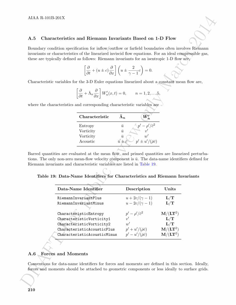
DRAFT

-For

publ

icre

view

only

Mar

ch20

14

AIAA R-101B-201X

A.5 Characteristics and Riemann Invariants Based on 1-D Flow

Boundary condition specification for inflow/outflow or farfield boundaries often involves Riemanninvariants or characteristics of the linearized inviscid flow equations. For an ideal compressible gas,these are typically defined as follows: Riemann invariants for an isentropic 1-D flow are,[

∂

∂t+ (u± c) ∂

∂x

](u± 2

γ − 1c

)= 0.

Characteristic variables for the 3-D Euler equations linearized about a constant mean flow are,[∂

∂t+ Λn

∂

∂x

]W ′n(x, t) = 0, n = 1, 2, . . . 5,

where the characteristics and corresponding characteristic variables are

Characteristic Λn W ′n

Entropy u p′ − ρ′/c2

Vorticity u v′

Vorticity u w′

Acoustic u± c p′ ± u′/(ρc)

Barred quantities are evaluated at the mean flow, and primed quantities are linearized perturba-tions. The only non-zero mean-flow velocity component is u. The data-name identifiers defined forRiemann invariants and characteristic variables are listed in Table 19.

Table 19: Data-Name Identifiers for Characteristics and Riemann Invariants


RiemannInvariantPlus u+ 2c/(γ − 1) L/TRiemannInvariantMinus u− 2c/(γ − 1) L/T

CharacteristicEntropy p′ − ρ′/c2 M/(LT2)CharacteristicVorticity1 v′ L/TCharacteristicVorticity2 w′ L/TCharacteristicAcousticPlus p′ + u′/(ρc) M/(LT2)CharacteristicAcousticMinus p′ − u′/(ρc) M/(LT2)

A.6 Forces and Moments

Conventions for data-name identifiers for forces and moments are defined in this section. Ideally,forces and moments should be attached to geometric components or less ideally to surface grids.

210

DRAFT

-For

publ

icre

view

only

Mar

ch20

14

AIAA R-101B-201X

Currently, the standard mechanism for storing forces and moments is generally through the Con-vergenceHistory_t node described in Section 12.3, either attached to the entire configuration(under CGNSBase_t, Section 6.2) or attached to a zone (under Zone_t, Section 6.3).

Given a differential force ~f (i.e., a force per unit area), the force integrated over a surface is,

~F = Fxex + Fy ey + Fz ez =∫

~f dA,

where ex, ey and ez are the unit vectors in the x, y and z directions, respectively. The momentabout a point ~r0 integrated over a surface is,

~M = Mxex +My ey +Mz ez =∫

(~r − ~r0)× ~f dA.

Lift and drag components of the integrated force are,

L = ~F · L D = ~F · D

where L and D are the unit vectors in the positive lift and drag directions, respectively.

Lift, drag and moment are often computed in auxiliary coordinate frames (e.g., wind axes orstability axes). We introduce the convention that lift, drag and moment are computed in the(ξ, η, ζ) coordinate system. Positive drag is assumed parallel to the ξ-direction (i.e., D = eξ); andpositive lift is assumed parallel to the η-direction (i.e., L = eη). Thus, forces and moments definedin this auxiliary coordinate system are,

L = ~F · eη D = ~F · eξ

~M = Mξ eξ +Mη eη +Mζ eζ =∫

(~r − ~r0)× ~f dA.

Lift, drag and moment coefficients in 3-D are defined as,

CL =L

12ρrefq

2refSref

CD =D

12ρrefq

2refSref

~CM =~M

12ρrefq

2refcrefSref

,

where 12ρrefq

2ref is a reference dynamic pressure, Sref is a reference area, and cref is a reference length.

For a wing, Sref is typically the wing area and cref is the mean aerodynamic chord. In 2-D, thesectional force coefficients are,

cl =L′

12ρrefq

2refcref

cd =D′

12ρrefq

2refcref

~cm =~M ′

12ρrefq

2refc

2ref

,

where the forces are integrated along a contour (e.g., an airfoil cross-section) rather than a surface.

The data-name identifiers and definitions provided for forces and moments and their associatedcoefficients are listed in Table 20. For coefficients, the dynamic pressure and length scales used inthe normalization are provided.

211

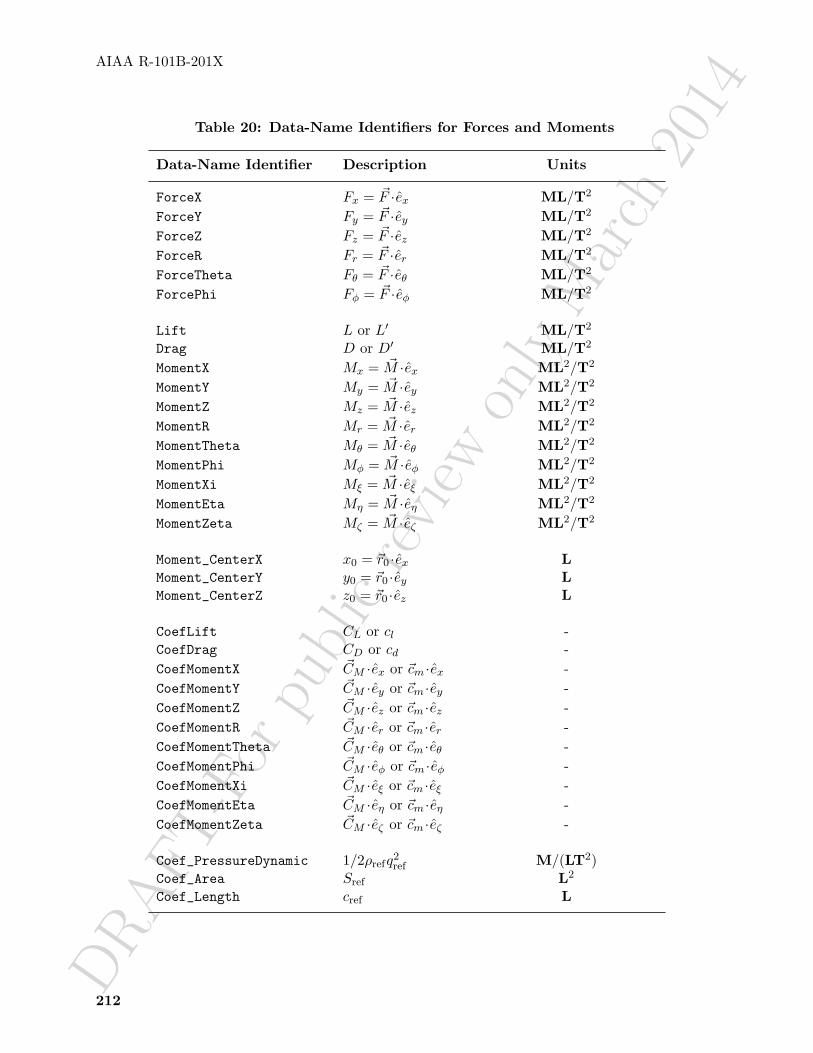
DRAFT

-For

publ

icre

view

only

Mar

ch20

14

AIAA R-101B-201X

Table 20: Data-Name Identifiers for Forces and Moments


ForceX Fx = ~F ·ex ML/T2

ForceY Fy = ~F ·ey ML/T2

ForceZ Fz = ~F ·ez ML/T2

ForceR Fr = ~F ·er ML/T2

ForceTheta Fθ = ~F ·eθ ML/T2

ForcePhi Fφ = ~F ·eφ ML/T2

Lift L or L′ ML/T2

Drag D or D′ ML/T2

MomentX Mx = ~M ·ex ML2/T2

MomentY My = ~M ·ey ML2/T2

MomentZ Mz = ~M ·ez ML2/T2

MomentR Mr = ~M ·er ML2/T2

MomentTheta Mθ = ~M ·eθ ML2/T2

MomentPhi Mφ = ~M ·eφ ML2/T2

MomentXi Mξ = ~M ·eξ ML2/T2

MomentEta Mη = ~M ·eη ML2/T2

MomentZeta Mζ = ~M ·eζ ML2/T2

Moment_CenterX x0 = ~r0 ·ex LMoment_CenterY y0 = ~r0 ·ey LMoment_CenterZ z0 = ~r0 ·ez L

CoefLift CL or cl -CoefDrag CD or cd -CoefMomentX ~CM ·ex or ~cm ·ex -CoefMomentY ~CM ·ey or ~cm ·ey -CoefMomentZ ~CM ·ez or ~cm ·ez -CoefMomentR ~CM ·er or ~cm ·er -CoefMomentTheta ~CM ·eθ or ~cm ·eθ -CoefMomentPhi ~CM ·eφ or ~cm ·eφ -CoefMomentXi ~CM ·eξ or ~cm ·eξ -CoefMomentEta ~CM ·eη or ~cm ·eη -CoefMomentZeta ~CM ·eζ or ~cm ·eζ -

Coef_PressureDynamic 1/2ρrefq2ref M/(LT2)

Coef_Area Sref L2

Coef_Length cref L

212

DRAFT

-For

publ

icre

view

only

Mar

ch20

14

AIAA R-101B-201X

A.7 Time-Dependent Flow

Data-name identifiers related to time-dependent flow include those associated with the storageof grid coordinates and flow solutions as a function of time level or iteration. Also included areidentifiers for storing information defining both rigid and arbitrary (i.e., deforming) grid motion.

Table 21: Data-Name Identifiers for Time-Dependent Flow

DataData-Name IdentifierType

Description Units

TimeValues real Time values TIterationValues int Iteration values -NumberOfZones int Number of zones used for each recorded

step-

NumberOfFamilies int Number of families used for each recordedstep

-

ZonePointers char Names of zones used for each recorded step -FamilyPointers char Names of families used for each recorded

step-

RigidGridMotionPointers char Names of RigidGridMotion structuresused for each recorded step for a zone

-

ArbitraryGridMotionPointers char Names of ArbitraryGridMotion structuresused for each recorded step for a zone

-

GridCoordinatesPointers char Names of GridCoordinates structuresused for each recorded step for a zone

-

FlowSolutionPointers char Names of FlowSolution structures usedfor each recorded step for a zone

-

OriginLocation real Physical coordinates of the origin beforeand after a rigid grid motion

L

RigidRotationAngle real Rotation angles about each axis of thetranslated coordinate system for rigid gridmotion

α

RigidVelocity real Grid velocity vector of the origintranslation for rigid grid motion

L/T

RigidRotationRate real Rotation rate vector about the axis of thetranslated coordinate system for rigid gridmotion

α/T

GridVelocityX real x-component of grid velocity L/TGridVelocityY real y-component of grid velocity L/TGridVelocityZ real z-component of grid velocity L/T


213

DRAFT

-For

publ

icre

view

only

Mar

ch20

14

AIAA R-101B-201X

Table 21: Data-Name Identifiers for Time-Dependent Flow (Continued)

DataData-Name IdentifierType

Description Units

GridVelocityR real r-component of grid velocity L/TGridVelocityTheta real θ-component of grid velocity α/TGridVelocityPhi real φ-component of grid velocity α/TGridVelocityXi real ξ-component of grid velocity L/TGridVelocityEta real η-component of grid velocity L/TGridVelocityZeta real ζ-component of grid velocity L/T

214

DRAFT

-For

publ

icre

view

only

Mar

ch20

14

AIAA R-101B-201X

B Structured Two-Zone Flat Plate Example

This section describes a complete database for a sample test case. The test case is compressibleturbulent flow past a flat plat at zero incidence. The domain is divided into two zones as shown inFigure 10. The interface between the two zones is 1-to-1.

Zone 125× 65× 3

Zone 249× 65× 3

-6

x, i

y, j

Symmetry Solid wall

Outflow Outflow

Inflow Outflow

Figure 10: Two-Zone Flat Plate Test Case

The database description includes the following:

• range of indices within each zone

• grid coordinates of vertices

• flowfield solution at cell centers including a row of ghost-cells along each boundary; theflowfield includes the conservation variables and a turbulent transport variable

• multizone interface connectivity information

• boundary condition information

• reference state

• description of the compressible Navier-Stokes equations including one-equation turbulencemodel

Each of these items is described in separate sections to make the information more readable. Thesame database is presented in each section, but only that information needed for the particularfocus is included. The overall layout of the database is presented in Section B.1.

All data for this test case is nondimensional and is normalized consistently by the following (dimen-sional) quantities: plate length L, freestream static density ρ∞, freestream static speed of sound c∞,and freestream static temperature T∞. The fact that the database is completely nondimensional isreflected in the value of the globally set data class.

B.1 Overall Layout

This section describes the overall layout of the database. Included are the cell dimension andphysical dimension of the grid, the globally set data class, the global reference state and flow-equations description, and data pertaining to each zone. Each zone contains the grid size, grid

215

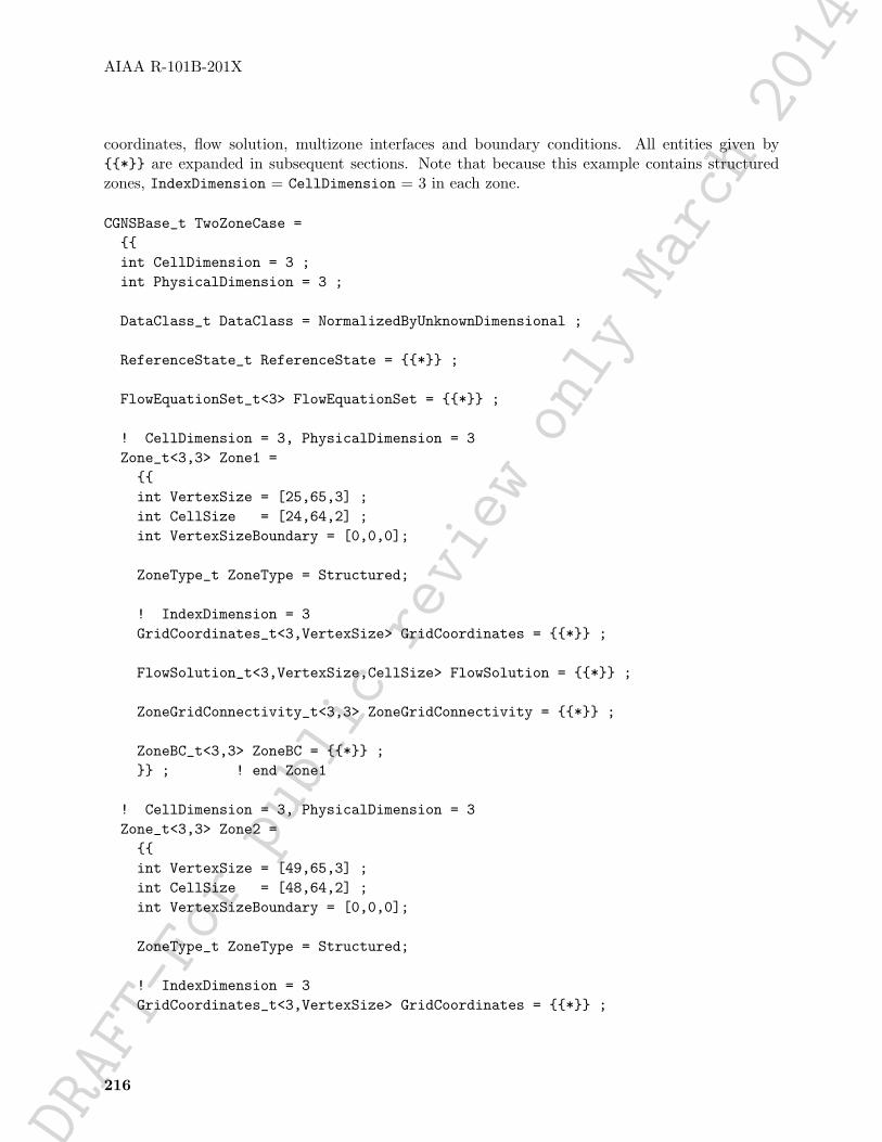
DRAFT-Forpublic

review

only


coordinates, flow solution, multizone interfaces and boundary conditions. All entities given by{{*}} are expanded in subsequent sections. Note that because this example contains structuredzones, IndexDimension = CellDimension = 3 in each zone.

CGNSBase_t TwoZoneCase ={{int CellDimension = 3 ;int PhysicalDimension = 3 ;

DataClass_t DataClass = NormalizedByUnknownDimensional ;

ReferenceState_t ReferenceState = {{*}} ;

FlowEquationSet_t<3> FlowEquationSet = {{*}} ;

! CellDimension = 3, PhysicalDimension = 3Zone_t<3,3> Zone1 ={{int VertexSize = [25,65,3] ;int CellSize = [24,64,2] ;int VertexSizeBoundary = [0,0,0];

ZoneType_t ZoneType = Structured;

! IndexDimension = 3GridCoordinates_t<3,VertexSize> GridCoordinates = {{*}} ;

FlowSolution_t<3,VertexSize,CellSize> FlowSolution = {{*}} ;

ZoneGridConnectivity_t<3,3> ZoneGridConnectivity = {{*}} ;

ZoneBC_t<3,3> ZoneBC = {{*}} ;}} ; ! end Zone1



! IndexDimension = 3GridCoordinates_t<3,VertexSize> GridCoordinates = {{*}} ;

216

DRAFT-Forpublic

review

only


FlowSolution_t<3,VertexSize,CellSize> FlowSolution = {{*}} ;

ZoneGridConnectivity_t<3,3> ZoneGridConnectivity = {{*}} ;

ZoneBC_t<3,3> ZoneBC = {{*}} ;}} ; ! end Zone2

}} ; ! end TwoZoneCase

B.2 Grid Coordinates

This section describes the grid-coordinate entities for each zone. Since the coordinates are allnondimensional, the individual DataArray_t entities do not include a data-class qualifier; instead,this information is derived from the globally set data class. The grid-coordinate entities for zone 2are abbreviated.





! IndexDimension = 3! VertexSize = [25,65,3]GridCoordinates_t<3, [25,65,3]> GridCoordinates ={{DataArray_t<real, 3, [25,65,3]> CoordinateX ={{Data(real, 3, [25,65,3]) = (((x(i,j,k), i=1,25), j=1,65), k=1,3) ;}} ;

DataArray_t<real, 3, [25,65,3]> CoordinateY ={{Data(real, 3, [25,65,3]) = (((y(i,j,k), i=1,25), j=1,65), k=1,3) ;}} ;

217

DRAFT-Forpublic

review

only


DataArray_t<real, 3, [25,65,3]> CoordinateZ ={{Data(real, 3, [25,65,3]) = (((z(i,j,k), i=1,25), j=1,65), k=1,3) ;}} ;

}} ; ! end Zone1/GridCoordinates}} ; ! end Zone1



! IndexDimension = 3! VertexSize = [49,65,3]GridCoordinates_t<3, [49,65,3]> GridCoordinates ={{DataArray_t<real, 3, [49,65,3]> CoordinateX = {{*}} ;DataArray_t<real, 3, [49,65,3]> CoordinateY = {{*}} ;DataArray_t<real, 3, [49,65,3]> CoordinateZ = {{*}} ;}} ; ! end Zone2/GridCoordinates

}} ; ! end Zone2}} ; ! end TwoZoneCase

B.3 Flowfield Solution

This section provides a description of the flowfield solution including the conservation variablesand the Spalart-Allmaras turbulent-transport quantity (ν). The flowfield solution is given at cellcenters with a single row of ghost-cell values along each boundary.

As with the case for grid coordinates, the flow solution is nondimensional, and this fact is derivedfrom the globally set data class. The normalizations for each flow variable are,

ρ′ijk =ρijkρ∞

, (ρu)′ijk =(ρu)ijkρ∞c∞

, (ρe0)′ijk =(ρe0)ijkρ∞c2

∞, ν ′ijk =

νijkc∞L

,

where primed quantities are nondimensional and all others are dimensional.

Only the Density entity for zone 1 is fully described in the following. The momentum, energy andturbulence solution are abbreviated. The entire flow-solution data for zone 2 is also abbreviated.

CGNSBase_t TwoZoneCase ={{

218

DRAFT

-For

publ

icre

view

only

Mar

ch20

14

AIAA R-101B-201X

int CellDimension = 3 ;int PhysicalDimension = 3 ;




! IndexDimension = 3! VertexSize = [25,65,3]! CellSize = [24,64,2]FlowSolution_t<3, [25,65,3], [24,64,2]> FlowSolution ={{GridLocation_t GridLocation = CellCenter ;

! IndexDimension = 3Rind_t<3> Rind ={{int[6] RindPlanes = [1,1,1,1,1,1] ;}} ;

! IndexDimension = 3! DataSize = CellSize + [2,2,2] = [26,66,4]DataArray_t<real, 3, [26,66,4]> Density ={{Data(real, 3, [26,66,4]) = (((rho(i,j,k), i=0,25), j=0,65), k=0,3) ;}} ;

DataArray_t<real, 3, [26,66,4]> MomentumX = {{*}} ;DataArray_t<real, 3, [26,66,4]> MomentumY = {{*}} ;DataArray_t<real, 3, [26,66,4]> MomentumZ = {{*}} ;DataArray_t<real, 3, [26,66,4]> EnergyStagnationDensity = {{*}} ;DataArray_t<real, 3, [26,66,4]> TurbulentSANutilde = {{*}} ;}} ; ! end Zone1/FlowSolution

}} ; ! end Zone1

Zone_t<3,3> Zone2 = {{*}} ;}} ; ! end TwoZoneCase

219

DRAFT-Forpublic

review

only


B.4 Interface Connectivity

This section describes the interface connectivity between zones 1 and 2; it also includes the k-planeperiodicity for each zone (which is essentially an interface connectivity of a zone onto itself). Eachinterface entity is repeated with the receiver and donor-zone roles reversed; this includes the periodick-plane interfaces. Since each interface is a complete zone face, the GridConnectivity1to1_tentities are named after the face.

Because of the orientation of the zones, the index transformation matrices (Transform) for allinterfaces are diagonal. This means that each matrix is its own inverse, and the value of Transformis the same for every pair of interface entities.


! ----- ZONE 1 Interfaces ------



! IndexDimension = 3, CellDimension = 3ZoneGridConnectivity_t<3,3> ZoneGridConnectivity ={{

! IndexDimension = 3GridConnectivity1to1_t<3> IMax = ! ZONE 1 IMax{{int[3] Transform = [1,2,3] ;IndexRange_t<3> PointRange ={{int[3] Begin = [25,1 ,1] ;int[3] End = [25,65,3] ;}} ;

IndexRange_t<3> PointRangeDonor ={{int[3] Begin = [1,1 ,1] ;int[3] End = [1,65,3] ;

220

DRAFT-Forpublic

review

only


}} ;Identifier(Zone_t) ZoneDonorName = Zone2 ;}} ;

GridConnectivity1to1_t<3> KMin = ! ZONE 1 KMin{{int[3] Transform = [1,2,-3] ;IndexRange_t<3> PointRange ={{int[3] Begin = [1 ,1 ,1] ;int[3] End = [25,65,1] ;}} ;

IndexRange_t<3> PointRangeDonor ={{int[3] Begin = [1 ,1 ,3] ;int[3] End = [25,65,3] ;}} ;


GridConnectivity1to1_t<3> KMax = ! ZONE 1 KMax{{int[3] Transform = [1,2,-3] ;IndexRange_t<3> PointRange ={{int[3] Begin = [1 ,1 ,3] ;int[3] End = [25,65,3] ;}} ;



}} ; ! end Zone1/ZoneGridConnectivity}} ; ! end Zone1

! ----- ZONE 2 Interfaces ------

! CellDimension = 3, PhysicalDimension = 3Zone_t<3,3> Zone2 ={{int VertexSize = [49,65,3] ;

221

DRAFT-Forpublic

review

only


int CellSize = [48,64,2] ;int VertexSizeBoundary = [0,0,0];


! IndexDimension = 3, CellDimension = 3ZoneGridConnectivity_t<3,3> ZoneGridConnectivity ={{

! IndexDimension = 3GridConnectivity1to1_t<3> IMin = ! ZONE 2 IMin{{int[3] Transform = [1,2,3] ;IndexRange_t<3> PointRange ={{int[3] Begin = [1,1 ,1] ;int[3] End = [1,65,3] ;}} ;

IndexRange_t<3> PointRangeDonor ={{int[3] Begin = [25,1 ,1] ;int[3] End = [25,65,3] ;}} ;


GridConnectivity1to1_t<3> KMin = ! ZONE 2 KMin{{int[3] Transform = [1,2,-3] ;IndexRange_t<3> PointRange ={{int[3] Begin = [1 ,1 ,1] ;int[3] End = [49,65,1] ;}} ;



GridConnectivity1to1_t<3> KMax = ! ZONE 2 KMax{{int[3] Transform = [1,2,-3] ;

222

DRAFT-Forpublic

review

only


IndexRange_t<3> PointRange ={{int[3] Begin = [1 ,1 ,3] ;int[3] End = [49,65,3] ;}} ;



}} ; ! end Zone2/ZoneGridConnectivity}} ; ! end Zone2


B.5 Boundary Conditions

Boundary conditions for the flat plate case are described in this section. The minimal informationnecessary is included in each boundary condition; this includes the boundary-condition type andBC-patch specification. The lone exception is the viscous wall, which is isothermal and has animposed temperature profile (given by the array temperatureprofile()). For all other boundaryconditions a flow solver is free to impose appropriate BC-data since none is provided in the following.The imposed BC-data for all cases should be evaluated at the globally set reference state, since noother reference states have been specified.

No boundary condition descriptions are provided for the multizone interface or for the k-planeperiodicity in each zone. All relevant information is provided for these interfaces in the GridCon-nectivity1to1_t entities of the previous section.

The practice of naming BC_t entities after the face is followed.



! ----- ZONE 1 BC’s ------

! CellDimension = 3, PhysicalDimension = 3Zone_t<3,3> Zone1 ={{int VertexSize = [25,65,3] ;int CellSize = [24,64,2] ;

223

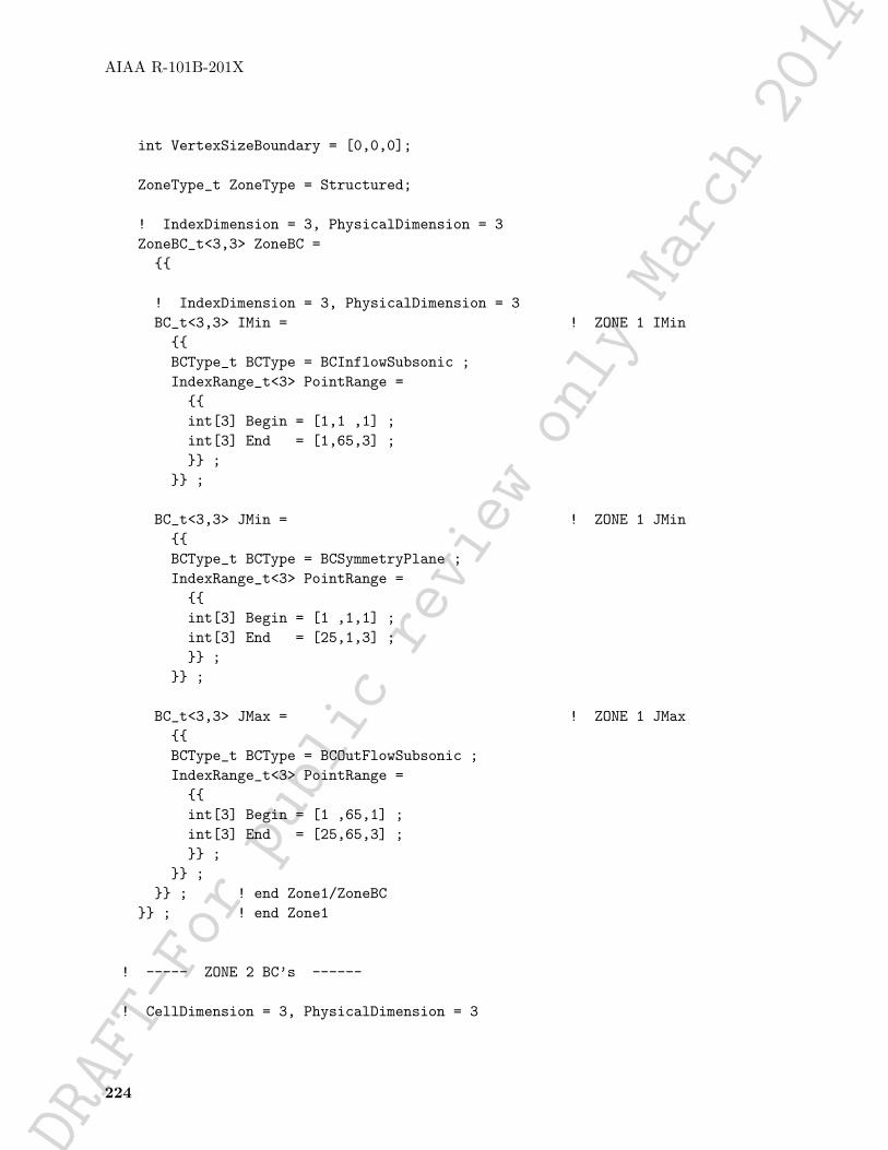
DRAFT-Forpublic

review

only


int VertexSizeBoundary = [0,0,0];


! IndexDimension = 3, PhysicalDimension = 3ZoneBC_t<3,3> ZoneBC ={{

! IndexDimension = 3, PhysicalDimension = 3BC_t<3,3> IMin = ! ZONE 1 IMin{{BCType_t BCType = BCInflowSubsonic ;IndexRange_t<3> PointRange ={{int[3] Begin = [1,1 ,1] ;int[3] End = [1,65,3] ;}} ;

}} ;

BC_t<3,3> JMin = ! ZONE 1 JMin{{BCType_t BCType = BCSymmetryPlane ;IndexRange_t<3> PointRange ={{int[3] Begin = [1 ,1,1] ;int[3] End = [25,1,3] ;}} ;

}} ;

BC_t<3,3> JMax = ! ZONE 1 JMax{{BCType_t BCType = BCOutFlowSubsonic ;IndexRange_t<3> PointRange ={{int[3] Begin = [1 ,65,1] ;int[3] End = [25,65,3] ;}} ;

}} ;}} ; ! end Zone1/ZoneBC

}} ; ! end Zone1

! ----- ZONE 2 BC’s ------

! CellDimension = 3, PhysicalDimension = 3

224

DRAFT-Forpublic

review

only


Zone_t<3,3> Zone2 ={{int VertexSize = [49,65,3] ;int CellSize = [48,64,2] ;int VertexSizeBoundary = [0,0,0];


! IndexDimension = 3, PhysicalDimension = 3ZoneBC_t<3,3> ZoneBC ={{

! IndexDimension = 3, PhysicalDimension = 3BC_t<3,3> IMax = ! ZONE 2 IMax{{BCType_t BCType = BCOutflowSubsonic ;IndexRange_t<3> PointRange ={{int[3] Begin = [49,1 ,1] ;int[3] End = [49,65,3] ;}} ;

}} ; ! end Zone2/ZoneBC/IMax

BC_t<3,3> JMin = ! ZONE 2 JMin{{BCType_t BCType = BCWallViscous ;IndexRange_t<3> PointRange ={{int[3] Begin = [1 ,1,1] ;int[3] End = [49,1,3] ;}} ;

! ListLength = 49*3 = 147BCDataSet<147> BCDataSet ={{BCTypeSimple_t BCTypeSimple = BCWallViscousIsothermal ;

! Data array length = ListLength = 147BCData_t<147> DirichletData ={{DataArray_t<real, 1, 147> Temperature ={{Data(real, 1, 147) = (temperatureprofile(n), n=1,147) ;}} ;

}} ;

225

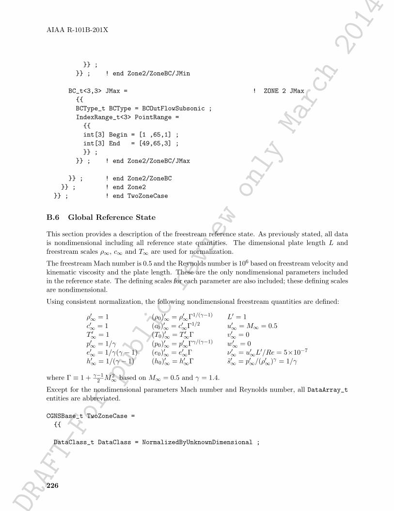
DRAFT-Forpublic

review

only


}} ;}} ; ! end Zone2/ZoneBC/JMin

BC_t<3,3> JMax = ! ZONE 2 JMax{{BCType_t BCType = BCOutFlowSubsonic ;IndexRange_t<3> PointRange ={{int[3] Begin = [1 ,65,1] ;int[3] End = [49,65,3] ;}} ;

}} ; ! end Zone2/ZoneBC/JMax

}} ; ! end Zone2/ZoneBC}} ; ! end Zone2


B.6 Global Reference State

This section provides a description of the freestream reference state. As previously stated, all datais nondimensional including all reference state quantities. The dimensional plate length L andfreestream scales ρ∞, c∞ and T∞ are used for normalization.

The freestream Mach number is 0.5 and the Reynolds number is 106 based on freestream velocity andkinematic viscosity and the plate length. These are the only nondimensional parameters includedin the reference state. The defining scales for each parameter are also included; these defining scalesare nondimensional.

Using consistent normalization, the following nondimensional freestream quantities are defined:

ρ′∞ = 1 (ρ0)′∞ = ρ′∞Γ1/(γ−1) L′ = 1c′∞ = 1 (c0)′∞ = c′∞Γ1/2 u′∞ = M∞ = 0.5T ′∞ = 1 (T0)′∞ = T ′∞Γ v′∞ = 0p′∞ = 1/γ (p0)′∞ = p′∞Γγ/(γ−1) w′∞ = 0e′∞ = 1/γ(γ − 1) (e0)′∞ = e′∞Γ ν ′∞ = u′∞L

′/Re = 5×10−7

h′∞ = 1/(γ − 1) (h0)′∞ = h′∞Γ s′∞ = p′∞/(ρ′∞)γ = 1/γ

where Γ ≡ 1 + γ−12 M2

∞ based on M∞ = 0.5 and γ = 1.4.

Except for the nondimensional parameters Mach number and Reynolds number, all DataArray_tentities are abbreviated.

CGNSBase_t TwoZoneCase ={{


226

DRAFT-Forpublic

review

only


ReferenceState_t ReferenceState ={{Descriptor_t ReferenceStateDescription ={{Data(char, 1, 10) = "Freestream" ;}} ;

DataArray_t<real, 1, 1> Mach ={{Data(real, 1, 1) = 0.5 ;DataClass_t DataClass = NondimensionalParameter ;}} ;

DataArray_t<real, 1, 1> Mach_Velocity = {{ 0.5 }} ;DataArray_t<real, 1, 1> Mach_VelocitySound = {{ 1 }} ;

DataArray_t<real, 1, 1> Reynolds ={{Data(real, 1, 1) = 1.0e+06 ;DataClass_t DataClass = NondimensionalParameter ;}} ;

DataArray_t<real, 1, 1> Reynolds_Velocity = {{ 0.5 }} ;DataArray_t<real, 1, 1> Reynolds_Length = {{ 1. }} ;DataArray_t<real, 1, 1> Reynolds_ViscosityKinematic = {{ 5.0E-07 }} ;

DataArray_t<real, 1, 1> Density = {{ 1. }} ;DataArray_t<real, 1, 1> LengthReference = {{ 1. }} ;DataArray_t<real, 1, 1> VelocitySound = {{ 1. }} ;DataArray_t<real, 1, 1> VelocityX = {{ 0.5 }} ;DataArray_t<real, 1, 1> VelocityY = {{ 0 }};DataArray_t<real, 1, 1> VelocityZ = {{ 0 }} ;DataArray_t<real, 1, 1> Pressure = {{ 0.714286 }} ;DataArray_t<real, 1, 1> Temperature = {{ 1. }} ;DataArray_t<real, 1, 1> EnergyInternal = {{ 1.785714 }} ;DataArray_t<real, 1, 1> Enthalpy = {{ 2.5 }} ;DataArray_t<real, 1, 1> EntropyApprox = {{ 0.714286 }} ;

DataArray_t<real, 1, 1> DensityStagnation = {{ 1.129726 }} ;DataArray_t<real, 1, 1> PressureStagnation = {{ 0.847295 }} ;DataArray_t<real, 1, 1> EnergyStagnation = {{ 1.875 }} ;DataArray_t<real, 1, 1> EnthalpyStagnation = {{ 2.625 }} ;DataArray_t<real, 1, 1> TemperatureStagnation = {{ 1.05 }} ;DataArray_t<real, 1, 1> VelocitySoundStagnation = {{ 1.024695 }} ;

DataArray_t<real, 1, 1> ViscosityKinematic = {{ 5.0E-07 }} ;}} ;

227

DRAFT-Forpublic

review

only



B.7 Equation Description

This section provides a description of the flow equations used to solve the problem. The flowequation set is turbulent, compressible 3-D Navier-Stokes with the Spalart-Allmaras (S-A) one-equation turbulence model. The thin-layer Navier-Stokes diffusion terms are modeled; only diffusionin the j-coordinate direction is included.

A perfect gas assumption is made with γ = 1.4; based on the normalization used in this database, thenondimensional scales defining γ are (cp)′ = 1/(γ−1) and (cv)′ = 1/γ(γ−1). The molecular viscosityis obtained from Sutherland’s Law. In order to nondimensionalize the viscosity formula, standardatmospheric conditions are assumed (i.e., T∞ = 288.15 K). A constant Prandtl number assumptionis made for the thermal conductivity coefficient; Pr = 0.72. The defining scales of Pr are evaluatedat freestream conditions; the nondimensional thermal conductivity is k′∞ = µ′∞(cp)′/Pr.

The Navier-Stokes equations are closed with an eddy viscosity assumption using the S-A model. Aturbulent Prandtl number of Prt = 0.9 is prescribed. All parameters not provided are defaulted.

Except for the nondimensional parameters γ and Pr, all DataArray_t entities are abbreviated.



! CellDimension = 3FlowEquationSet_t<3> FlowEquationSet ={{int EquationDimension = 3

! CellDimension = 3 ;GoverningEquations_t<3> GoverningEquations ={{GoverningEquationsType_t GoverningEquationsType = NSTurbulent ;



DataArray_t<real, 1, 1> SpecificHeatRatio ={{

228

DRAFT-Forpublic

review

only


Data(real, 1, 1) = 1.4 ;DataClass_t DataClass = NondimensionalParameter ;}} ;

DataArray_t<real, 1, 1> SpecificHeatRatio_Pressure = {{ 2.5 }} ;DataArray_t<real, 1, 1> SpecificHeatRatio_Volume = {{ 1.785714 }} ;}} ;

ViscosityModel_t ViscosityModel ={{ViscosityModelType_t ViscosityModelType = SutherLandLaw ;

DataArray_t<real, 1, 1> SutherLandLawConstant = {{ 0.38383 }} ;DataArray_t<real, 1, 1> TemperatureReference = {{ 1.05491 }} ;DataArray_t<real, 1, 1> ViscosityMolecularReference = {{ 5.0E-07 }} ;}} ;

ThermalConductivityModel_t ThermalConductivityModel ={{ThermalConductivityModelType_t ThermalConductivityModelType =ConstantPrandtl ;

DataArray_t<real, 1, 1> Prandtl ={{Data(real, 1, 1) = 0.72 ;DataClass_t DataClass = NondimensionalParameter ;}} ;

DataArray_t<real, 1, 1> Prandtl_ThermalConductivity = {{ 1.73611E-0.6 }} ;DataArray_t<real, 1, 1> Prandtl_ViscosityMolecular = {{ 5.0E-0.7 }} ;DataArray_t<real, 1, 1> Prandtl_SpecificHeatPressure = {{ 2.5 }} ;}} ;

TurbulenceClosure_t TurbulenceClosure ={{TurbulenceClosureType_t TurbulenceClosureType = EddyViscosity ;

DataArray<real, 1, 1> PrandtlTurbulent = {{ 0.90 }} ;}} ;

TurbulenceModel_t<3> TurbulenceModel ={{TurbulenceModelType_t TurbulenceModelType =OneEquation_SpalartAllmaras ;


229

DRAFT

-For

publ

icre

view

only

Mar

ch20

14

AIAA R-101B-201X

}} ; ! end FlowEquationSet}} ; ! TwoZoneCase

230

cgns standard interface data structures - higher...

Documents