Liquidity of the government of Canadasecurities market: stylised facts and some market microstructure

comparisons to the United States treasury market

Toni Gravelle*

Financial Markets DepartmentBank of Canada

(E–mail: tgravelle@bank-banque-canada.ca)

Abstract

The aim of this paper is to study how liquidity in the Government of Canada (GoC) securities markethas evolved over time and to determine what factors tend to influence the level of liquidity in the GoCsecurities market, especially in comparison with the US Treasury market. The principal structuraldifferences between the Canadian and US markets are: the extent of fragmentation in the GoCsecurities market is higher; activities in the interest rate futures market in Canada is significantlylower; transparency for customers in Canada is lower; and market makers in Canada are subject to amuch smaller and less heterogeneous customer base. Using data for the GoC securities market, it isshown that the outstanding amount of securities has a negative effect on bid-ask spreads and a positiveeffect on turnover ratio. This supports the hypothesis that an increase in effective supply enhancesmarket liquidity. Interest rate volatility has a positive effect on bid-ask spreads and on trading volumein the futures market. This supports the hypothesis that an increase in inventory risk of market makersleads to wider bid-ask spreads in the cash market and higher activities in the futures market forhedging purposes. Other possible factors which have improved liquidity of the GoC securities marketin recent years include a decrease of concentration in secondary markets, increases in inter-dealerbroker trades and non-resident participation.

* The author would like to acknowledge the help of Zahir Lalani who provided many invaluable comments and alsoprovided the author with a link to the government securities trading community. This study is intended to make theresults of Bank research available in preliminary form to other analyst to encourage discussion. The views expressed arethose of the author. The analysis and conclusions offered in this study do not represent the official views of the Bank ofCanada or the Department of Finance.

1

1. Introduction and motivation

In this study we examine the liquidity of the Government of Canada (GoC) securities market. In mostcountries, the government securities (GS) market is often viewed as the most important financialmarket, since GS perform several key functions that tend to enhance a country’s economic well being.The GS market is of particular interest to central banks since it is often the market in which theyperform their domestic monetary operations, where they extract information on future movements ofinterest rates and where governments raise funds, the latter of interest to central banks with fiscalagency responsibilities. Furthermore, because of their virtually riskless nature, GS function as thepricing benchmark for several other fixed-income securities and serve as collateral (or as part ofregulatory capital requirements) for various financial intermediaries, enabling them to finance theiroperations. More generally, since fixed-income markets possess most of the structural and institutionalcharacteristics as GS markets, a greater understanding of how GS markets function provides centralbanks with a better understanding of fixed-income markets. Clearly, the liquidity of GS marketsshould be important to authorities interested in maintaining or enhancing the functioning of thesemarkets and financial markets in general.

There are three distinct channels through which market liquidity has an impact on a central bank’score activities. First, market liquidity will have an impact on monetary policy formulation andimplementation activities. Central banks are keenly interested in extracting information from financialasset, since their prices reveal information on current and future monetary conditions, which can beused in the formulation and implementation of monetary policy. However, market liquidity affectshow information gets embedded in prices (i.e. it affects the price discovery process). Thus, to theextent that varying levels of market liquidity may impinge on the market’s ability to aggregateindividual investor information into prices (i.e. market efficiency),1 it effects the central bank’sconfidence in its expectational measures. Moreover, the transmission of monetary policy actions tolonger maturity fixed-income instruments may be impinged by low levels of market liquidity. Marketliquidity also has a more direct impact on monetary policy implementation in that it may affect theefficacy of a central bank’s open-market operations.

Second, under certain circumstances, market illiquidity is often a symptom, if not a cause, of systemicfinancial crises or disruptions. Depending on the level of market liquidity, stressful shocks to financialmarkets may be amplified rather than dampened. This amplification coupled, in some cases, with thepresence of “feedback trading”, can lead to liquidity or solvency problems at key financialintermediaries, which, if held unchecked, could lead to payment system disruptions and/or a collapsein credit allocation.2 Therefore, fluctuations in market liquidity may have direct impact on a centralbank’s activities both as a lender of last resort and in its supervision (or monitoring) of (prudential)financial stability. Further, in calculating the potential market risks, VaR models ignore liquidation orliquidity risks, defined as the risk of being unable to liquidate a position in a timely manner at areasonable price. Specifically, the VAR methodology assumes that prices vary in a continuousmanner, ignoring the possibility that price movements may be discontinuous (or “gap”) in anenvironment where liquidation risks are prominent. Since risk management systems at most financialintermediaries are now based on the VaR methodology, this shortcoming may cause or aggravatemarket disruptions.3

Third, in its role as fiscal agent, a central bank will share the government’s desire to minimise debtservice costs. Secondary market liquidity tends to make it easier for governments to issue largeamounts of debt at relatively low costs since investors feel more confident in their ability to purchase

1Markets are termed efficient when prices in these markets reflect all information available to market participants.Muranaga and Shimizu (1997) discuss how changes in market liquidity affect the price discovery process and marketefficiency.

2Muranaga and Shimizu (1997) have a nice discussion of how changes in market liquidity affect market stability.

3See Muranaga and Ohsawa (1997) for a broader discussion of liquidation or liquidity risks and risk models.

2

the product in the primary market and subsequently trade the product in a liquid secondary market. Incarrying out its role as fiscal agent, therefore, a central bank would work in conjunction with thegovernment to enhance the integrity and efficiency of the government securities market.

In this study, a liquid market is defined as one in which trading is immediate, and where large tradeshave little impact on current and subsequent prices or bid-ask spreads. Thus market liquidity, which isdistinct from the monetary or aggregate liquidity more familiar to central bankers trained inmacroeconomics, can be defined over four dimensions: Immediacy, depth, width (bid-ask spread), andresiliency. Immediacy refers to the speed with which a trade of a given size at a given cost iscompleted. Depth refers to the maximal size of a trade for any given bid-ask spread. Width refers tothe costs of providing liquidity. Resiliency refers to how quickly prices revert to original (or“fundamental”) levels after a large transaction. However, in the context of government securitiesmarkets, liquidity is better thought of in terms of the cost of supplying immediacy. Since most GSmarkets are multi-dealer markets, all trades are as immediate as the time it takes to agree to trade witha dealer.4 That is, market makers are providers of immediacy. The costs of this immediate trade willvary depending on the size and direction of the trade and on variations in the market makers’ costs toproviding this immediacy. This in turn implies that liquidity will vary. As this discussion makes clear,the various dimensions of liquidity interact with each other (e.g. for a given (immediate) trade, widthwill generally increase with size or, for given bid-ask spread, all transaction under a given size can beexecuted (immediately) without price or spread movement).

This study will focus on how liquidity in the GoC securities market has evolved over time and ondetermining what factors tend to influence the level of liquidity in the GoC securities market. With theuse of trading volume and bid-ask data as well as a series of stylised facts, we are able to examine howliquidity in the GoC securities market has changed over time. In order to sharpen our analysis of whichstructural or institutional factors have a significant influence on GoC market liquidity, we proceed bydrawing comparisons to a GS market that is similar in many dimension to that of the GoC securitiesmarket. By doing so, we reduce the dimensionality of our problem. That is, one can think of this studyas trying to implement a controlled experiment in which one controls for all but one (or a few) of thefactors that may have an impact on the results. Thus, by comparing two GS markets that arestructurally very similar, but with differing levels of liquidity, we can control the number of factorsthat differ across markets and that potentially have an impact on liquidity. Since they have manystructural characteristics in common, comparisons are made between the GoC securities market andthe market for U.S. Treasuries.

The study will focus on how variations in four microstructural characteristics, specific to GS markets,impact the level of liquidity in GS markets. These factors are: Debt instrument characteristics,competition and concentration, inventory management (or inventory control costs), and transparencyor information considerations. In particular, we focus on these four structural characteristics in order tounderstand how the evolution of liquidity is influenced by changes in these structural factors over timeand how differences in these structural factors may cause market liquidity to differ across countries.

The term debt instrument characteristics is used to identify a series of factors – specific to governmentfixed-income instruments – that tend to affect a debt instrument’s intrinsic tradeability (such as, thefactors affecting its (effective) supply and demand, its distribution among market participants, how itis initially issued, and its fungibility to name a few). Since liquidity in over-the-counter GS markets is,in essence, supplied by dealers, it is important to understand what influences their incentives to makemarkets and supply immediacy.5 Therefore the other three factors influence the market maker’s ability

4In contrast to most equity markets, investors (customers) in GS markets do not place limit orders – standing offers totrade at a given price – with dealers, they only place market orders with dealers, orders that are immediately executedagainst a dealers quote. Thus, from the investor’s perspective, all trades are immediate.

5Throughout this study the term dealer is often used in place of market maker. In reality, not all GS dealers can beconsidered market makers. However, in this study dealers, unless specified otherwise, are assumed to refer to marketmakers.

3

or costs to provide liquidity. Competition and concentration is a term used to encompass factorsrelated to the number of competing dealers, the level of dealer competition in the GS market, themanner in which dealers strategically interact or compete, and the size and diversity of the customerbase. Inventory management include factors affecting the market maker’s ability to provideimmediacy such as, the costs associated with hedging or re-balancing their positions. Finallytransparency and information refers to the factors pertaining to the transparency of the tradingenvironment (such as the publication of transaction prices/quantities and real-time quotations) and theinteraction of public information and private information, where public information includesmacroeconomic news releases and private (or strategic) information includes such things as a dealer’ssuperior knowledge of their own order flow and inventories.

Throughout this study, we endeavour to relate our findings and descriptions of the stylised facts to theideas developed in market microstructure literature.6 The next section provides a comparisons of themarket structures for the U.S. and Canadian GS markets. Section 3 presents a series of stylised factsdescribing the evolution of GoC securities market liquidity. Section 4 presents some more formal testsof certain market liquidity hypotheses, while Section 5 briefly summarises our findings and providesadditional remarks on how the observed stylised facts my have influenced GS market liquidity inCanada.

2. Market structure

In this section, we provide a review of the institutional structure for the Government of Canadasecurities market. Generally, the structure of the Canadian market is quite similar to the U.S. Treasurymarket in that trading in both markets takes place in a continuous, over-the-counter competitivemulti-dealer market.7 Since details on the structure of the U.S. and Canadian market are readilyavailable from various sources,8 the first part of this section will only provides a summary tablereviewing the market structures that are common to both government securities markets. The secondpart highlights the important institutional/structural differences that exist in both markets.

2.1 Similarities

The market structures that are common to both government securities markets are identified in Table 1below, where the first column identifies the common component and the second and third columnidentify the slight discrepancies that are assumed to have negligible effects on market liquidity.

6See O’Hara (1995) for a primer on the market microstructure literature.

7See Dattels (1995) for more details on the various types of continuous market structures.

8See Inoue (1999) for institutional details of the Canadian and US markets, Fleming and Remolona (1997), Sundaresan(1997), Singleton (1995) and Stigum (1990) for details of the U.S. Treasury market only, while we refer you to Harveyand Boisvert (1998), Bank of Canada Review (1996), Branion (1995) and Fettig (1994) for some details on the GoCsecurities market.

4

Table 1

Common market structures

Common Canada1 US2

Primary market

Primary Dealer (PD) System3

Securities distributed at auctions (withan active pre-auction when issuedmarket)

• Only PDs can submit bids4

• Top 10 PDs win 75% of auctionproceeds (1998 data)

• Only index-linked bonds usesingle-price auctions; all other usecompetitive bid format.

• Greater number of dealers otherthan PDs can submit bids

• PDs accounted for 72% of auctionwinnings; top 10 PD accounted for50% of that

• All fixed coupon instruments usesingle-price auctions

PDs in both countries have similaroffsetting obligations and incentives

• Two tier system

Similar minimum capital requirementsfor PD status (with commercial bankssatisfying Basel Capital Accord)

• Must be IDA registered dealers • Must be SEC registered dealers

Secondary market

OTC multiple dealer, quote drivenmarket: customers must contact dealersfor quotes and carry out transaction.Dealers can trade via customer marketor interdealer market

• Securities listed on NYSE, butvolume negligible

Primary dealers account for majority ofturnover

27 PDs; approx. 170 investmentdealers;5 5 interdealer brokers (IDBs)

32 PDs; 1,700 broker/dealers; 6 IDBs

• Interdealer trading is eitherconducted directly or via a “blind”interdealer broker system

• A little over 50% of PD trading iswith customers

Repo and Strip trading active

Book-entry clearing and settlementsystem similar

Settlement: T+2 shorter maturities; T+3longer maturities

Settlement: T+1

Tax and accounting systems verysimilar

1 Not that since the study was written, the primary dealer structure in Canada has changed. Please see the Bank of Canadaweb page (www.bank-banque-canada.ca) for details on the rules of participation in primary market. 2 Most of these stylisedfacts paper in Flaming and Remolona (1997). 3 See Goldstein and Folkerts-Landau (1994) for details of a primary dealersystem.). 4 Under the new primary dealer structure in Canada, customers may submit bids via PDS. 5 Source: InvestmentDealers Association (IDA) of Canada.

5

2.2 Differences

In this section we outline the more substantial differences in market structure that exists between theGoC and U.S. GS markets. This section provides a “snap-shot” of the GoC securities market structurerather than description of how it has evolved over time. As mentioned in the introduction, weconcentrate on the structural differences that pertain to the four broad factors that are believed to havea direct impact on market liquidity for OTC government security markets. Note that little effort ismade, in this section, to examine how the differing GS market structures impact market liquidity.Rather the structural differences are simply stated here, while their effects on liquidity are examinefurther in Sections 4 and 5.

2.2.1 Size of markets

The most obvious difference between the U.S. Treasury and Government of Canada securities marketsis their size. Table 2 presents the trading volume and amount outstanding of marketable governmentsecurities in each country. It is clear that the amount outstanding and volume of transactions (turnover)in Canada is significantly smaller than in the U.S. Indeed, the stock of marketable securities in theU.S. is 12 times that of Canada’s while trading volume in the U.S. is 14 times greater than it is inCanada.

In terms of turnover, the Canadian government securities market is vastly inferior to that of the U.S.market. On the other hand, so is Canada’s stock of government securities outstanding. Althoughaggregate turnover data is often used as a rough measure for the liquidity of a GS market, this measureis likely influenced to a certain extent by the size of the market itself and thus should be normalised insome way. A normalised measure of aggregate turnover, that attempts to controls for the size of themarket, is the turnover ratio, defined as turnover divided by the stock outstanding.9 The turnover ratiofor each country is presented in Table 2. It is clear that when using this normalised measure ofturnover, the apparent differences in trading activity (or the size of the markets) are greatly reduced,with Canada’s turnover ratio slightly less than that of the U.S.

Table 2

Size statistics for U.S. and Canadian government securities markets*

(USD billions)

Data Canada U.S.

Stock Outstanding 290.5 3,456.8

Turnover Volume 5,552.9 75,901.0

Turnover Ratio 19.1 21.9

* Source: BoJ/BIS market liquidity study based on 1997 data. An exchange rate US$1.43 CAD was used to convert intoUS dollars.

Before moving on to describe the other microstructural differences that exist between both countries,one should note that differences in the size of the markets themselves may unavoidably be a factorgenerating differences in liquidity and that differences in the microstructural factors may only have,relative to the size differences, second order effects on liquidity. Alternatively, the difference inmarket size may be the underlying cause of the structural or institutional differences that exists acrosscountries. The smaller size of the customer base for GoC securities is certainly reliant on the size of

9It is not clear, however, whether or not the turnover ratio defined in this study can be used to compare liquidity acrosscountries. We discuss this in more detail in Section 3. Note that other studies have attempted to control for the size effectsby normalising by GDP figures.

6

the GoC securities market. Thus it may be argued that by comparing the GoC securities market to theU.S. Treasury market, we are not controlling for (eliminating) the most important structural factoraffecting liquidity and that we would be better off making comparisons with a GS market of similarsize but with perhaps more divergent microstructures.10 In order to mitigate this criticism, we attemptto control for the size difference between the markets by normalising by the stock of outstanding GSwhere appropriate. Moreover, our examination of the changes in liquidity over time is not based on thecross-country differences and thus stands on its own.

2.2.2 Debt instrument characteristics: issuance patterns, fragmentation and effective supply

One of the structural differences between the two markets is bond issuing practices. First, the U.S.Treasury market issuance practice can be described as “regularised”. That is, since the mid-70’s therehas been a regular issuance of bonds with a limited set of maturities in relatively large size.11

Moreover, the maturity of new issues matches, in general, the original maturity of retiring issues. InCanada, however, it was not until 1992, that the GoC bond market took on a “regularised” pattern.12

Until that time, GoC bond issuances in terms of timing, size and maturity was influenced by marketpreferences and conditions.13 As well, some existing bond issues that had a coupon rate close to yieldsprevailing in its maturity class were sometimes reopened, but a good number of issues were notreopened, many of which became small, illiquid, “orphaned” issues. This resulted in a highlyfragmented stock of bonds. Remnants of this practice are still apparent in the current stock of bonds.For example, as of the end of 1997 there were 31 fixed- coupon bonds currently still outstanding thatwere issued with an original maturity outside the current key maturity classes of 2, 5, 10, and 30 years.These issues had original terms to maturities that ranged between 19- and 25-years. Of these, 19 issueshave an amount outstanding less then US$1 billion (CAD) and none are greater than US$3 billion(CAD), which is a fraction of the current benchmark sizes of US$7 to 10 billion (CAD).

Gravelle (1998) argues that though dealer markets are better suited than auction-agency markets tohandle multiple security market making, a (too) high degree of fragmentation does eventually have anegative impact a dealer’s market making capabilities. When market makers hold a large number ofinstruments in their inventory, this increases their financing requirements, adds to their (costly)inventory control activities (including hedging activities), and consequently hinders their ability toprovide liquidity.

Table 3 presents some statistics on the fixed-coupon instruments for the two countries. Though theU.S. stock of fixed-coupon debt outstanding is about 13 times larger than that of Canada’s, it has only2.7 times the number of issues outstanding, indicating that Canada has a proportionally much largernumber of issues outstanding. Moreover, assuming that the issuance practices and the amountoutstanding of fixed-coupon debt remains constant over time in Canada, the steady state number ofbond issues outstanding would total 34, which is more than half the number issues outstanding at the

10The U.K. GS market, has a slightly larger stock of outstanding marketable government securities and has trading volumewhich is in the same range as the GoC securities market, thus would be a better size controlled comparator. The onlycountry that comes close to the U.S. GS market in terms of outstanding stock of securities is the Japanese GS market.

11Three-year Treasury notes were recently dropped from the set of maturities issued. The Treasury over the years has alsodiscontinued the issuance of 7-year notes in 1993, 4-year notes in 1991, and 20-year bonds in 1986.

12See Branion (1995) for some further details on the change in issuance practices commencing in 1992.

13Also, the continued issuance of some bonds through syndication (until 1992), in which a higher commission was paid onissues with longer terms to maturity, tended to skew the issuance process towards longer maturity bonds. Moreover, thiscaused the stock of bonds outstanding to have irregular original maturities.

7

end of 1997. The average issue size, defined as the outstanding stock divided by the number of issues,tends to capture these facts and thus provides a rough measure of debt stock fragmentation.14

Table 3

Debt stock statistics for U.S. and Canadian bond markets(USD billions)

Canada US1

Fixed-coupon stock outstanding 204.6 2,693.4

Number of issues 77 206

Average issue size 2.6 13.1

Average benchmark or on-the-run issue size 6.42 15.6

1 Source: BoJ/ECSC market liquidity study based on 1997 data. Excludes index-linked and zero couponinstruments. 2 Excludes no-longer issued 3-year maturity.

However, as previously mentioned, in 1992 the Government of Canada adopted several initiatives thathave basically brought its issuance practices in line with that of the U.S. Treasury. These initiativesincluded a commitment to large benchmark issues, a regular and transparent issuance calendar for 2, 5,10, and 30 year bonds, and common coupon payment dates. Over the years, the target sizes of thesebenchmark issues have been increased with the aim of improving issue liquidity. The currentbenchmark sizes range between US$5 and US$7 billion (US$7-10 billion CAD).15 The recentinitiation of large bond benchmarks explains, in part, why the average issue size is approximately 2/5the size of the current benchmark in Canada while in the U.S., it is a little more than 4/5 that of thecurrent on-the-runs. This is due to the fact that the average issue size is also a weighted average ofcurrent and past issues sizes. Therefore, these ratios not only provide an indication of how fragmentedthe Canadian market is versus the U.S., they also provide an indication of how gradual the increase inthe on-the-run issue size has been in the U.S. relative to the increase in GoC bond issue size.

Though the bond issuance practices for GoC securities have adopted most of the characteristics of theU.S. Treasury’s bond issuance practices (i.e. the regular issuance of large benchmark securities), thereremains one aspect of the GoC primary market that differs. The large GoC bond sizes are achieved viasuccessive, regular reopenings after the initial auction, whereas the U.S. Treasury issues new largebenchmarks at almost every auction.16,17 This implies that a GoC bond does not achieve its so-called

14The average issue size for other countries is also available. Inoue (1999) provides data on average issue size that includesindex-linked, zero- and fixed-coupon securities. These are US$5.5, US$8.2, US$5.6 and US$14.3 billion (USD) for Italy,Japan, UK, and U.S. government securities markets respectively.

15The targeted size of the 10-year and 30-year benchmark issues increased from US$5-6, US$6-8, US$6--9, toUS$7-10 billion in 1992, 1993, 1994 and 1996 respectively. Similarly, the target size of the 5-year benchmark bond issuerose from US$4-5, US$5-7, US$6-9, to US$7-10 billion in those same years, while the target size of the 2-year bondwent from US$3, US$4, US$4-6, to US$7-10 billion.

16In the end, the number of reopenings is conditional on the number of reopening required to achieve the annuallyannounced target size, on whether or not the issue is not too far outside its “key” maturity class and on the size of theindividual auctions which are in turn dependent on the total amount of stock being issued within the (budgetary) year.Throughout most of the period since 1992, this has implied that 2-year bonds are reopened once after the initial offering,5 and 10-year bonds are reopened 3 times and 30-year bonds or reopened 3 to 5 times. Note that the 2, 5, and 10-yearbonds are auctioned quarterly (implying a new 2-year every six months and new 5- and 10-years every year) while the30-year bond is, as of 1998, auctioned semi-annually.

17The U.S. Treasury has, at times, chosen to reopen certain fixed-coupon issues (notably 10-year notes).

8

on-the-run liquidity status, as the most liquid security in its maturity class, until its accumulated sizenears that of the old benchmark (usually on its second-to-last or last reopening). This also implies thatthe transfer of the on-the-run liquidity status (and the liquidity premium attached to the security’sprice) from the old to the new benchmark is not usually as discrete for GoC bonds, as it is for U.S.coupon securities.

What effect does the practice of reopening issues have on liquidity? If the transfer of benchmark statusand in turn the transfer of the liquidity premium (in terms of price) associated with the benchmarkbond is as discrete is it is for the one time issue of new bonds (like U.S. Treasury securities), then thisissuance technique likely has little consequence on GS market liquidity. However, if this issuancepractice succeeds in creating two bonds in the same maturity class with benchmark status and liquidityfor even a short period, this may have a positive impact on market liquidity since this increases thenumber of actively traded securities. This assumes that the increase in the number of active bonds doesnot take away from the liquidity of off-the-run bonds (i.e. assumes that liquidity can be concentrated inmore than one bond or that it is not a zero sum game across the spectrum of bonds within a maturityclass). To our knowledge, there has not been any empirical or theoretical research in this area, thusleaving the effect of this issuance practice on market liquidity unresolved.

The issuance practices of the GoC treasury bills (t-bills) have changed relatively little since themid-1980s. Until late 1997, t-bills were auctioned weekly with 3, 6, and 12 month maturities, with the3-month t-bill being the largest of the three maturities to be issued. Since then t-bills have been issuedon a bi-weekly frequency. The stock of GoC marketable debt had, until recently, continuouslyincreased allowing for an ever increasing stock of t-bills. However, due to a decision to increase theproportion of the fixed-rate debt to 2/3 of the gross government debt in 1996 and the fact that theGovernment of Canada has been operating with budgetary surpluses, the stock of t-bills have been in asteady decline since 1996.

2.2.3 Inventory risks and costs: futures markets

Though large issue sizes and regular issuance calendars are institutional factors underpinning aspectsof market liquidity we term debt instrument characteristics, other important institutional differencesbetween U.S. and Canadian government securities markets fall under what we term inventory riskmanagement. Specifically, we focus on the relative state of development of interest rate futuresmarkets across the two countries, since a particularly important consideration in a dealer’s cost inmaking markets are its costs associated with hedging and financing large inventories of governmentsecurities.

The repo market also plays an integral role in hedging and financing large inventories of governmentsecurities and thus would also affect the market maker’s inventory management risks and costs and, inturn, their costs to providing immediacy. However, the sample of data available for the Canadian repomarket is relatively short (starting in 1994). (Moreover, a BIS CGFS working group is currentlystudying repo markets with the results of their research efforts being released sometime in late 1998 orearly 1999.) As such, this study will concentrate on examining the interaction between futures marketactivity and GoC securities market liquidity.

In Canada, there currently exist two actively traded domestic exchange-traded interest rate futurescontracts. Both of these are traded on the Montréal Exchange. The cash delivery three-monthCanadian Banker’s Acceptance Futures (BAX) and the physical delivery ten-year Government ofCanada Bond Futures (CGB). Recent average daily volume (number of contracts) figures for thesecontracts ranged around 31,000 for the BAX and 8,500 for the CGB.18 Though the BAX and CGB areconsidered to be successful futures contracts in terms of trading activity by Canadian standards, they

18The five-year Government of Canada Bond Futures (CGF) and one-month Canadian Banker’s Acceptance Futures(BAR) contracts are recent additions to the futures exchange and rarely average more than a few hundred contracts tradeda day. They are therefore not considered, for the purposes of this study, active.

9

generally fall considerably short of the level of activity of similar contracts traded on Australian,French, Japanese, German, UK, and U.S. exchanges. In comparison to the Canadian daily volumefigures, recent figures for the ten-year Treasury notes contract (traded on the CBoT) range from75,000 to 200,000 contracts traded, while the three-month Eurodollar contract (traded on the CME)has ranged from 550,000 to 800,000 contracts traded. Both of the instrument’s characteristics and theway they are traded are similar to the CGB and BAX contracts. In fact, these contracts were modelledoff those traded at the CME/CBoT. In absolute terms, the Canadian futures trading activity is about1/25 the size of comparable U.S. futures activity. Moreover, there is a smaller number of activeinterest rate futures traded in Canada. In the U.S., there are at least 14 interest rate futures contracts (6on CME, 8 on CBoT). This greater breath of products in the U.S. (not to mention the other U.S. dollarinterest rate futures traded on other exchanges in and outside the U.S.), coupled with the lower tradingintensity in Canada, indicates that the development of the interest rate futures market in Canada fallssignificantly short of the U.S. futures market.

Section 3, below, presents some stylised facts for the evolution of trading activity for both futurescontracts in Canada.

2.2.4 Transparency

Public access to real-time quote, price, and trade information or ex-post transaction information isoften sparse in most government securities markets, the exception being the U.S. governmentsecurities market where real time market transparency is provided by GovPX Inc.19 Inoue (1999)provides a comparison of the level of transparency provided in a group of G5 countries (includingCanada and the U.S.). The data indicates that the level of transparency provided to customers (thepublic) in Canada lies at the lower end of the spectrum in terms of transparency while the U.S. marketlies near the upper end. Specifically, customers in Canada must, in general, directly contact a seriesdealers to ascertain firm best bid and ask quotations. Moreover, historical intraday transaction pricesand quantities are not generally available to the public, though indicative quotations from a selectnumber of dealers are available intradaily (to the public) from information vendors (such asBloomberg, Reuters or Telerate). With GovPX, the customer side of the cash U.S. governmentsecurities market is much more transparent. [Note that there are currently efforts under way in Canadato develop a screen-based information system similar to GovPX (tentatively named CanPX).] In theinterdealer market, both the Canadian and American markets offer comparable levels of transparencywith both markets being served by interdealer broker system which provides dealers with realtimescreen-based firm quotation and transaction data.

2.2.5 Competition and concentration

Though both the U.S. and Canada have primary dealer systems in which primary dealers tend to alsobe market makers in the secondary government securities market, the number and size (in terms ofcapitalisation or operations) of these primary dealers differ substantially across countries. In Canada,27 primary dealers are, as is the case in the U.S. with 32 primary dealers, on one side of the majorityof government securities transaction. In Canada 10 of these primary dealers are involved in over 80%of the secondary market turnover reported by primary dealers. Unfortunately, data on the level of U.S.dealer competition is not available.

The size and diversity of the customer base faced by market makers in a GS market may also play arole in their ability to provide liquidity. Therefore, concentration in the customer base should also beconsidered when comparing market structures. Anecdotal evidence indicates that although there hasbeen a globalisation of financial markets over the years, the dealers in Canada are subject to a muchsmaller and less heterogeneous customer base for GoC securities than there exist for U.S. Treasuries.

19See Fleming and Remolona (1997) for a description of GovPX data. Note that the Italian GS market is also verytransparent (see Inoue (1999) for some details).

10

Evidence presented in Section 3 indicates that the customer base in Canada has diversified over the1990s with an increasing proportion of non-residents being included in the customer turnover data. Ofthe domestic customer base that actively trades their portfolios, it has been suggested by marketparticipants that it is proportionally smaller than the active U.S. customer base and that it is dominatedby a handful of large institutions. These large institutions tend to use their market power to force thedealers to aggressively compete for their business. Of the other smaller, relatively active domesticcustomers, there tends to be less diversity in trading strategies and market views; this is in part due tothe small number of constituent players. The U.S. GS market, on the other hand, not only attracts alarge international base of customers, due to the depth of this market and the U.S. dollar’s role as areserve currency, it also has, arguably, the largest and must heterogeneous domestic customer base.

3. Secondary market liquidity for GoC securities in the 1990s

In this section we offer some time-series measures for the liquidity of the Government of Canadasecurities market. An often used measure of market liquidity in GS markets is trading volume (orturnover), which measures the accumulated value of transactions over a fixed period. On the otherhand, a measure of market liquidity that has a strong theoretical appeal is one that would more closelyapproximate trading intensity20. Theory predicts that market makers, who provide liquidity byabsorbing short-term order imbalances that disappear once the other side of the market emerges, willbenefit from a higher level of trading intensity since they will wait a shorter period of time to takeadvantage of a rebalancing or offsetting order. Therefore, the aggregate turnover ratio, defined as totalturnover divided by the stock of securities, tends to do a better job of capturing the level of liquidityprevalent in a market than simple turnover, since it better approximates trading intensity. If turnoverincreased without a corresponding increase in the total stock of GS, this would imply, in principal, anincrease in (aggregate) trading frequency. At the end of the first subsection we discuss some of thelimitations of using aggregate turnover ratio data as an approximation for the level of liquidity in GSmarkets. Optimally, one requires data on the number of transactions as well as the size of thetransactions for each individual government security to get more precise measure of trading intensityand liquidity. However, given data availability limitations, we use aggregate turnover ratio data as aproxy for the evolution of market liquidity in Canada under the assumption that the dispersion oftrading activity across outstanding GoC securities remains relatively constant over time.

The level of trading intensity is also reflected in the dealers quoted bid-ask spread. Sinceinventory-control or rebalancing risks diminish as trading intensity increases so too does theinventory-control component of the spread. However, the spread is in many ways a better proxy forliquidity than the (aggregate) turnover ratio measure since the spread reflects not only the tradingintensity of the instrument, but other factors such as adverse selection, transparency regimes, anasset’s price volatility, dealer competition as well as the other (unobserved) factors influencing marketmaking costs. As such, we also present some evidence on the evolution of market liquidity based onquoted bid-ask spreads which are assumed to better reflect the transaction costs charged by marketmakers to investors demanding immediacy. Though spread data is available at the daily frequency forGoC t-bills, detailed high frequency data for Government of Canada bonds is not available.

Because there exists a link between the market makers’ ability to manage its inventory risks andfutures market liquidity, we also present some trading statistics for interest rate futures that trade onthe Montréal Exchange.

20Amihud and Mendelson (1986) show that in equilibrium, liquidity of an asset is correlated with its trading frequency.Datar et al. (1998) suggest that the turnover rate of an asset, defined as the number (of units) of the asset traded dividedby the stock outstanding of this asset, has several advantages over the more commonly used quoted bid-ask spreadsproxy, one of which being its direct relation to the trade frequency of the asset.

11

3.1 Government of Canada secondary market turnover over time

An overview of the evolution of the trading volume over time and across types of GoC marketparticipants is presented in what follows. We will start by discussing the time series properties of totaltrading volume as reported to the Bank of Canada by primary dealers.21 Figure 1 presents both thebond and t-bill total weekly trading volume (with the eight-week moving average depicted by the thickline). This figure indicates that the bond trading volume has been trending upward, untilapproximately the fourth quarter of 1997, where it has since plateaued. The volume of transactions inthe treasury bill market had increased from 1990 to early 1996. Since that time, the trading volume fort-bills has declined substantially to levels comparable to that in 1990.22

The implication drawn from Figure 1 for the evolution of market liquidity, at least in terms of anindicative measure such as turnover, is that the GoC bond market has since the early 1990s becomeincreasingly more liquid while the t-bill market has seen a continual decline in trading activity sincemid 1996, after an extended period of increasing liquidity.

3.1.1 Effective supply conditions

What are some of the factors that have led to this increasing trend in GoC bond turnover and the recentdecline treasury bill trading volumes. Gravelle (1998) and Miyanoya et. al. (1997) suggest that onefactor affecting the trading activity, and in turn the liquidity, of debt instruments is its effective supply.Effective supply is defined as the supply of the security in the hands of active market participants(which is equal to the total supply less the supply that is in the hands of buy- and-hold marketparticipants).23 It is argued that as the effective supply of these instruments increases, so should itstrading activity. Effective supply, in turn, tends to increase with the amount outstanding of theseinstruments. Gravelle (1998) suggests that a greater effective supply of individual benchmark bondsproduces a positive participation externality on the trading activity of these instruments.24 This impliesthat, ceteris paribus, trading activity for these instruments should increase (decrease) more quicklythan the rise (fall) in their issue size. We will denote this as the effective supply hypothesis.

As mentioned in Section 2.2, the issuing practices in the GoC bond market underwent a restructuringaimed at building up distinct benchmark bond maturities of significant size. This change in regimeprovides us with a specific event in which to gather evidence concerning the hypothesis that increasesin an issue’s size has positive effect on turnover. Similarly, on-the-run t-bill issue size has decreasedsince 1996 as the government moved to issuing a higher proportion of its debt as fixed rate (coupon)debt and as government funding requirements decreased.

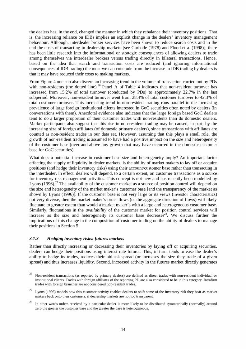
Some indication of the effects of increased GS issue size is illustrated in Figures 2 and 3. The toppanels of Figures 2 and 3 present the average weekly turnover (averaged over a month) and theamount outstanding (stock) of GoC bonds and t-bills respectively. Figure 2 indicates that the averageweekly turnover for bonds has generally trended upward in tandem with the increase in outstanding

21Each of the primary dealers submits a money market and bond market trading report that covers one-week offixed-income trading. The trading volume is segmented into several categories that include a primary distributors salesand purchases from other investment dealers, interdealer brokers, banks, other domestic market participants (customers),and non-resident market participants. The trading volume is also segmented across trading instruments such asGovernment of Canada marketable securities, provincial marketable securities, corporate fixed-income instruments andasset-backed securities to name a few.

22Note that, currently, the turnover data is available at no higher than the weekly frequency. Also, collection of weeklyGoC turnover data began in 1989.

23Effective supply may be increased by repo or securities lending transaction where securities are lent out of buy-and-holdportfolios. Symmetrically, effective supply diminishes as GS securities are stripped.

24This positive participation externality explanation is similar to the idea that a feedback loop between trading volume andmarket liquidity explains the fact that trading tends to concentrate at particular times of the day in the Admati andPfleiderer (1988) study.

12

stock and benchmark size of GoC bonds. Similarly, Figure 3 indicates that the t-bill turnover tends tobe highly correlated with the stock of these instruments. (Although there was no formal policy inplace, average on-the-run t-bill issue size did increase as a result of greater government funding needs,before 1996.).25 The bottom panels present the monthly turnover ratio, defined as the average monthlyturnover divided by the stock of the GoC securities, for both the bond and t-bill market. The rise in thebond turnover ratio is an indication that trading volume has increased more than one-for-one with theincrease in the size of the outstanding stock of bonds. Thus, the evidence presented in Figure 2 isconsistent with the effective supply hypothesis. The same can be said for t-bill trading volume. As thestock of t-bills increased from 1990 to 1995, so too did the turnover ratio (see bottom panel of Figure3). After 1995, however, the transaction volume for t-bills has decline somewhat more quickly thanthe stock supporting the hypothesis that there exist a positive issue size externality.

Aggregate turnover ratio caveat

In the above analysis, we used aggregate turnover ratio data under the assumption that these data do abetter job of capturing the level of liquidity prevalent in a market than raw turnover data. However, anincrease in the aggregate turnover ratio does not necessarily imply that each individual securityexperienced an increase in trading activity (or trading frequency). It’s possible that certain individualsecurities experienced a reduction in trade frequency, as aggregate trade frequency increased. Whatdoes this mean for market-wide liquidity? When there is no decline in trading activity for anyindividual security, an increase in aggregate turnover translates into an increase in market-wide tradingintensity and liquidity. But when certain securities experience a decline in trading activity as otherexperience an increase in trading frequency, it is not clear whether the market as a whole has becomemore liquid or whether some individual securities have become more liquid at the expense of others.Without data on the individual securities trading activity, a measure of liquidity at the disaggregatedlevel is not possible. Moreover, the effective supply hypothesis is based on the relation between theissue size and trading activity of individual instruments. Therefore, it is not clear that, without theassumption that the dispersion of trading activity across the stock of GS remains relatively constantover time, increases in the turnover ratio reflect increases in trading frequency (and, in turn, marketliquidity) arising from the effective supply consequences of larger individual benchmark issue sizes.(In Section 4 we suggest a more powerful method to test the effective supply hypothesis.)

As the preceding discussion makes clear, when using aggregated turnover data, one must makeassumptions about possible changes in the dispersion of trading activity across the stock of individualsecurities. It also implies that cross-country comparisons of market liquidity based on aggregateturnover ratio data may be biased since the dispersion of trading activity across the stock of GSinvariably differs across countries. For example, two countries with equal aggregate turnover ratiosmay in fact have significantly different (aggregate) trading intensities, when trading activity (andturnover) in one country is concentrated in a smaller number of instruments relative to the other.Moreover, as noted by Inoue (1999), the effective turnover ratio may be affected by the central bank’sor the government’s practice of holding till maturity a large proportion of the stock of marketablesecurities. Given that these practices vary across countries, this implies that the turnover ratios are notdirectly comparable across countries. However, within a country, under the assumption that thedispersion of trading activity across its stock of GS is constant or relatively persistent, aggregateturnover ratios are likely a good approximation for changes in trading intensity and liquidity (overtime), and a useful indicator for effective supply effects.

25Since there were no changes in the issuance frequency (until late 1997) of t-bills and since t-bill securities roll-overrelatively quickly, an increase in on-the-run issue size would necessarily occur in tandem with an increase in governmentfunding financed with t-bill securities.

13

3.1.2 Inventory control/rebalancing

Since the GoC market is an OTC dealer market where market makers are the predominate supplier ofliquidity, it is important to understand how dealers maintain their desired level of inventory. Do theylay off (acquire) their unwanted (wanted) inventory positions through interdealer brokers or do theytrade bilaterally with other dealers or customers? Inventory management via interdealer brokers(IDBs) has very different informational consequences than inventory management that occurs viabilateral transactions. Thus the price formation process will differ between markets with differentlevels of interdealer broking. An advantage of trading via interdealer brokers is that it gives dealers theability to rebalance there inventory position quickly. If dealers are continuously hit by customer ordersof varying size and direction, the process of rebalancing their inventory positions is shorter viainterdealer broking trades than via direct bilateral interdealer trades (or waiting for offsettingcustomers trades). Thus, in theory, the greater use of interdealer trade should increase the dealersability to absorb order flow and in turn improve the dealers ability to provide liquidity. However, asthe work of Lyons (1996) suggests, the interdealer broker market is also an avenue where dealersextract information on aggregate order flow. Therefore the increasing use of interdealer brokers mayreflect an endogenously (or exogenously) driven change in the level of aggregate order flowtransparency. This section tries to shed light on the evolution of dealers’ position control activities inthe GoC market.

The first panel in Table 4 presents the average turnover of primary dealer (PD) trading conducted withvarious types of counterparties, as a per cent of total PD trading. The percentages are averaged oversub-periods in order to provide a sense of the evolution the market. The bottom panel in Table 4presents the average percentage of total interdealer trading that occurs through interdealer brokers(IDBs) and the average percentage of non-resident trading as a proportion of total customer trading.Note also the customer figures presented in Panel A include non-resident turnover and thus thepercentages add up to a figure that is greater than 100.

Table 4

Proportion of total primary dealer trading by counterparty

1991-93 1994-96 1997-98

Panel A: Two-way trading (%)

IDBs 30.6 37.2 39.3

Other dealers directly 15.8 10.2 7.1

Non-residents 15.2 19.7 22.7

Customers 53.7 52.6 53.6

Panel B: Within category trading (%)

IDB/total interdealer 65.8 78.5 84.7

Non-resident/total customer 28.4 37.5 42.3

Figure 4 displays graphically the data summarised in Panel A of Table 4. As is evident from the tableand figure, there is a clear rapid increase in the use of interdealer brokers on the part of primarydistributors (the irregular dashed line). Most dealers suggest that the decrease in broker fees over theyears is likely the main contributing factor to the increasing use of interdealer brokers. Nonetheless,the increasing use of IDBs does imply an increasing level of anonymous trading taking place amongthe dealers. Moreover, interdealer broker trades tend to be more numerous and at pre-set sizes thandirect interdealer trading or trades with customers. The trade size in the interdealer broker market alsovaries little over time when compared to the trade size variation observed by dealers when tradingbilaterally with customers or other dealers. These two facts imply that even though the decline inbroker fees may have been the impetus for the increasing use of IDBs, this increasing use of IDBs by

14

the dealers has, in the end, changed the manner in which they rebalance their inventory positions. Thatis, the increasing reliance on IDBs implies an explicit change in the dealers’ inventory managementbehaviour. Although, interdealer broker services have been shown to reduce search costs and in theend the costs of transacting in dealership markets [see Garbade (1978) and Flood et a. (1998)], therehas been little research into the informational or strategic consequences of allowing dealers to tradeamong themselves via interdealer brokers versus trading directly in bilateral transactions. Hence,based on the idea that search and transaction costs are reduced (and ignoring informationalconsequences of IDB trading) the most we can conclude from the increase in IDB trading by dealers isthat it may have reduced their costs to making markets.

From Figure 4 one can also discern an increasing trend in the volume of transaction carried out by PDswith non-residents (the dotted line).26 Panel A of Table 4 indicates that non-resident turnover hasincreased from 15.2% of total turnover (conducted by PDs) to approximately 22.7% in the lastsubperiod. Moreover, non-resident turnover went from 28.4% of total customer turnover to 42.3% oftotal customer turnover. This increasing trend in non-resident trading runs parallel to the increasingprevalence of large foreign institutional clients interested in GoC securities often noted by dealers (inconversations with them). Anecdotal evidence also indicates that the large foreign based GoC dealerstend to do a larger proportion of their customer trades with non-residents than do domestic dealers.Market participants also suggest that this rise in non-resident trading may be caused, in part, by theincreasing size of foreign affiliates (of domestic primary dealers), since transactions with affiliates arecounted as non-resident trades in our data set. However, assuming that this plays a small role, thegrowth of non-resident trading is assumed to have had a positive impact on the size and heterogeneityof the customer base (over and above any growth that may have occurred in the domestic customerbase for GoC securities).

What does a potential increase in customer base size and heterogeneity imply? An important factoreffecting the supply of liquidity in dealer markets, is the ability of market makers to lay off or acquirepositions (and hedge their inventory risks) using their account/customer base rather than transacting inthe interdealer. In effect, dealers will depend, to a certain extent, on customer transactions as a sourcefor inventory risk management activities. This concept is not new and has recently been modelled byLyons (1996).27 The availability of the customer market as a source of position control will depend onthe size and heterogeneity of the market maker’s customer base [and the transparency of the market asshown by Lyons (1996)]. If the customer base is not very large or its views (investor characteristics)not very diverse, then the market maker’s order flows (or the aggregate direction of flows) will likelyfluctuate to greater extent than would a market maker’s with a large and heterogeneous customer base.Similarly, fluctuations in the availability of the customer market for position control services willincrease as the size and heterogeneity its customer base decreases28. We discuss further theimplications of this change in the composition of customer trading on the ability of dealers to managetheir positions in Section 5.

3.1.3 Hedging inventory risks: futures markets

Rather than directly increasing or decreasing their inventories by laying off or acquiring securities,dealers can hedge their positions using interest rate futures. This, in turn, tends to ease the dealer’sability to hedge its trades, reduces their bid-ask spread (or increases the size they trade of a givenspread) and thus increases liquidity. Second, increased activity in the futures market directly generates

26Non-resident transactions (as reported by primary dealers) are defined as direct trades with non-resident individual orinstitutional clients. Trades with foreign affiliates of the reporting PD are also considered to be in this category. Intrafirmtrades with foreign branches are not considered non-resident trades.

27Lyons (1996) models how this customer activity enables dealers to shift some of the inventory risk they bear as marketmakers back onto their customers, if dealership markets are not too transparent.

28In other words orders received by a particular dealer is more likely to be distributed symmetrically (normally) aroundzero the greater the customer base and the greater the base is heterogeneous.

15

trading volume in the cash market due to arbitrage transactions. Thus, well developed and liquidfutures markets tend to enhance the liquidity of the underlying cash GS market. In this subsection, weinvestigate the evolution of interest rate futures turnover in Canada.

Figures 5 and 6 display the average daily volume (over a month) and month-end open interest for allthe BAX and CGB contracts outstanding from January 1990 to September 1998. These figuresillustrate that the BAX contract is clearly the more active of the two interest rate futures contracts withopen interest and trading volume figures approximately 4 to 6 times greater than the CGB futures (interms of number of contracts). One of the more interesting features depicted in these figures is thetendency of these futures contracts to reach plateaus in terms of trading activity. For example, both theBAX and CGB volume remained range bound till approximately early-1997, after having increasedsubstantially from 1993 till mid-1994. After sharply increasing over a brief period in early-1997, thevolume figures for the CGB contract again remained range bound till August 1998. Therefore, theretends to be some persistence in futures trading activity. That is to say, once an increase in tradingactivity does occur, for whatever reason, the level of activity does not revert to the low levels thatpreceded the increase. This is consistent with the hypothesis that high trading activities areself-enforcing or self-sustaining.29 To elaborate, there is a persistence to the level of trading activitybecause the higher trading activity attracts market participants that previously found the market tooinactive to participant in, which in turn increases trading activity and attracts more market participantsand so on.

The growth in trading activity in both the BAX and CGB contracts in 1993-1994 and in the BAX for1997 tend to coincide with an anticipated increases in interest rates and/or with a rise in interest ratevolatility (or uncertainty). Some support for this hypothesis is presented in Figure 7 where the monthlythree-month Banker’s Acceptances and ten-year bond yields are displayed in the thicker lines whiletheir daily observations are displayed in the thinner lines. Specifically, three-month and ten-year yieldsincreased considerably during 1994 while three-month rates in Canada increased in 1997-1998.Though ten-year yields steadily decreased through most of 1997-1998, this was also a period in whichthe Asian financial crisis came to the fore, perhaps explaining in part the 1997 rise in CGB activity. Asindicated in Figures 5 and 6, the most striking increasing in trading activity for both the CGB and theBAX contracts occurred in August-September 1998. August 1998 is the month that the Canadiancurrency came under extreme pressure with the BoC raising its policy rate by a 100 basis points,where ten-year yields rose more than 50 basis points after declining for more than a year, and in whichthe Asian financial crisis took on a more global flavour as Russia devalued its currency. This cursoryanalysis implies that the increase in futures activity may be linked to an increase in hedging activity bydealers and other market participants due to rising interest rates risks or increases in interest ratevolatility. Note also that investors who expect debt instrument prices to decline (or expect interestrates to rise) would find it considerably easier to “go short” in the futures market rather than theunderlying cash market due to less onerous margin requirements. However, this discrepancy inspeculative trading activity between the futures and cash market is not as pronounced for investorswishing to “go long” based on expectations of declining interest rates. This structural asymmetry inthe ease with which a market participant can short an instrument could explain the increase in futuresactivity during periods of rising (expected) interest rates and is not necessarily related to marketparticipants’ hedging activity when faced with increased volatility.30

Boisvert and Harvey (1998) also suggest that the recent increase trading activity in BAX futures is inpart due to the decline in the supply of treasury bills that has occurred since mid-1996. (Compare theamount of t-bill’s outstanding in Figure 3 to BAX open interest levels, Figure 5, during the 1996-1998

29Pagano (1989) and Admati and Pfleiderer (1988) considers questions related to this self-sustaining or feedback aspect ofmarket liquidity.

30However, a well-developed repo market makes it easier for market participant, dealers in particular, to short the cashinstrument. This, in turn, reduces the margin-related asymmetry that exist between the cash and futures market forinvestors wishing to “go short.”

16

period.) They suggest that investors, interested in taking (speculative) positions in the money market,have increasingly tended to invest in the BAX market rather than the treasury bill market in order toavoid technical problems linked to the t-bills’ dwindling supply.

Recent conversation with dealers suggests a third explanation for the 1997-1998 rise in tradingactivity. They mentioned that the arrival of additional “locals” from Chicago and France in theMontréal trading pits may be in part responsible for the increase in BAX futures activity.31 Also, it wasnoted that the sudden increase in CGB activity was due to the arrival foreign investors (such as hedgefunds) who participate in futures markets only after the volume of transaction crosses a criticalthreshold (e.g. 10,000 contracts per day).

3.2 Competition/concentration

Increased market maker competition is generally assumed to enhance market liquidity.32 Intuitively,market makers will compete with each others for order flow for two reasons. First an increasingnumber of transaction for a given bid-ask spread will increase market making trading volume andprofits and second, the larger the market maker’s share of aggregate order flow, the more precise is themarket maker’s proprietary information on the securities’ expected price movements, the greater itsproprietary trading profits (which are distinct from its market making profits). However, as is the casein goods markets, the predominate way market makers compete for order flow is by setting the best(lowest) price, which in terms of government securities markets means the best (narrowest) bid-askspread. And, because narrower bid-ask spreads are generally a reflection of the costs of immediacy,this implies that increased competition leads to greater liquidity.

Given the above discussion, it is clear that changes in the level of dealer concentration over time maybe one of the contributing factors explaining the evolution of GoC securities market liquidity. InCanada, the government securities industry has undergone a series of mergers among domestic dealers(and Banks) since 1987. One of the ongoing concerns of the authorities has been the effects of thesemergers on the integrity of the secondary market for Canadian government securities. It is believedthat a reduction in the number of active market maker dealers has or will eventually cause a reductionin the level of market liquidity.

In the industrial organisation literature there are several measures of market concentration available. Inthis study we calculate three measures, the 6– and 10-firm concentration ratios and the Herfindahlindex. These concentration measures, presented in Table 5, are calculated in terms of each dealer’sshare of yearly secondary bond market turnover from 1993 to the second quarter of 1998.33,34 Thesedata indicate a declining trend in secondary market concentration during a period where two majormergers, among the top tier of domestic primary dealers, occurred and where four foreign baseddealers gained primary dealer status.

Specifically, on September 1994 two primary dealers, that ranked among the top 12 in terms of 1993secondary bond market turnover, merged, while on September 1996, another merger occurred betweentwo firms that ranked among the top 8 in terms of 1995 secondary bond market turnover. Further,

31Locals in futures markets act in a similar way to market makers.

32One should note, however, that it is not necessarily the case that a greater number of market makers leads to greatercompetition. Dutta and Madhavan (1997) show that collusive (non-competitive) outcomes are possible independent of thenumber of market makers.

33The firm concentration ratios measure the sum of the market share for the top 6 or 10 primary dealers in terms of theirsecondary market turnover. The Herfindahl index is defined as the sum of the squared market shares of all reportingprimary dealers. See Tirole (1988) for details.

34Dealer concentration is, perhaps, better measured in terms a dealers share of customer turnover, rather than customer plusinterdealer turnover, since this would be a cleaner measure of the actual level of competition that exists for customerorder flow.

17

three foreign based dealers gained primary dealer status on November 1995, while another gained PDstatus on October 1994.35 Note also that 6 other foreign dealers had attained PD status before 1993.While some of these dealers have subsequently dropped out of the PD ranks, two of these have seentheir share of secondary market trading activity increase to the point where they are now rank amongthe top echelon of primary dealers.

In the top panel of Table 5, the concentration statistics for 1994 and 1996 are calculated assuming thatthe merged firms remained separate trading entities for the entire year while the bottom panelcombines the firms to form one trading entity throughout the year. Because the mergers occurredtwo-thirds of the way through the year,36 actual concentration statistics should in reality lie somewherein between these figures. Thus, by weighting the top and bottom 1994 and 1996 measures by theproportion of the year that the firms reported their trading data as separate entities, we have adjustedthe estimates for the concentration statistics to better reflect this fact. These calculations are presentedin brackets.37

The data indicates that the entree of new dealers or the capture of greater market share by existingforeign based dealers has had a greater impact on concentration measures than the occurrence of twomergers among relatively large PDs during the sample period. These data also support the widelyadhered to view that gains in market share arising from mergers in the securities industry are, at best,fleeting. A combined firm’s market share is never expected to equal the simple addition of theindividual pre-merger market shares of each firm since large clients prefer to spread their businessamong several firms (in order, among other things, to better hide their trading strategies).

Table 5

Measures of concentration in secondary bond market turnover

Year 6 Firm concentration ratio 10 Firm concentration ratio Herfindhal index

1993 0.647 0.898 0.09071994 0.627 (0.638) 0.886 (0.892) 0.0878 (0.0899)1995 0.618 0.840 0.08171996 0.614 (0.626) 0.798 (0.810) 0.0787 (0.0821)1997 0.597 0.841 0.08151998 Q2 0.607 0.834 0.0817

1994* 0.660 0.905 0.09401996* 0.651 0.835 0.0889

3.3 Bid-ask spreads over time

One measure of market liquidity often utilised is some measure of bid-ask spreads. As mentioned inthe introduction, the bid-ask spread reflects the costs to the dealers in providing immediacy. Thesecosts include, inventory management costs, trading costs, and costs associated with trading with a

35Note that since dealers have to meet certain trading activity requirements to get accorded PD status, it implies that theyhad maintained a threshold level of secondary (and primary) market activity over an extended period preceding the datethey become PDs. This implies that the PD in question was likely taking away market share from existing PDs before itofficially joined the PD ranks.

36Note also that, before these firms started reporting the trading volume as one entity, there was likely a period of severalweeks for which these firms’ trading desks were already behaving cooperatively (or as one trading desk).

37Moreover, this declining trend has occurred even as the number of primary bond market distributors/ dealers declinedfrom 48 in January of 1993 to 27 in the second quarter of 1998. Nonetheless, the dealers that lost their PD statusgenerally lost it because their behaviour was not consistent with that of market makers. Specifically, their primary andsecondary market trading activity was in fact minuscule in comparison to the remaining PD.

18

better informed investor (adverse-selection costs).38 Given the discussion in the previous subsection,the spread may also be affected by the level of competition among dealers.

Recent conversations with dealers indicate that benchmark bond spreads through most of the 1990shave averaged 2 cents for the 2-year, 3 to 5 cents for the 5-year, 5 cents for the 10-year and 7-10 centsfor the 30-year for every US$100 face value. These are quoted spreads for transaction up to theUS$100 million range. (Non-benchmark or off-the-run securities are quoted with somewhat higherspreads.) Unfortunately, high frequency time series bond spread data were not available for this study.

Data at a daily frequency are available for quoted treasury bill spreads. Figure 8 presents the weeklyaverage of daily observations of the 90-day t-bill spreads in terms of yield from January 1990 toOctober 1998, while Figure 9 adds the 180 and 360-day bid-ask t-bill spreads to the 90-day spreadspresented in Figure 8. Of the three maturities, the 90-day t-bill tends to have the narrowest spread, areflection of its greater amount outstanding, its greater turnover and, thus, its greater liquidity onaverage. An examination of Figures 7 and 8 highlights the correlation between sudden increases in the3-month yields and the sudden increase in the bid-ask spreads for 90-day treasury bills. These areapparent in 1992, in the early part of 1995 and again in late 1997 early 1998. There is also a sharpincrease in spreads again in September to October of 1998. It is clear that an increase in interest ratevolatility or uncertainty has a direct impact on the market makers willingness (or costs) to providingliquidity. As 3-month interest rates increase in a sudden manner, so do the spreads. This increase in thecost of immediacy supplied by market makers is a reflection of the higher inventory risk managementcosts they face. As interest rate uncertainty/volatility increases, dealers will tend to manage theirposition more closely or, alternatively, they will reduce their position altogether. This in turn leads to areduction in their ability to supply immediacy. Second, higher interest rate volatility will tend toreduce the order flow that dealers observe which in turn reduces the dealer’s ability to manage theirpositions. This too has a negative impact on the dealer’s costs of supplying immediacy and in turn apositive impact on the bid-ask spreads they quote. In summary, market makers will widen their quotedspreads when faced with increased inventory risks as their inventory-control component of the spreadincrease. Moreover, it is unlikely that other components of the spread (adverse selection, and tradingcosts) would vary over such a brief period.

This observed increase in t-bill spreads is not unlike the intraday widening of spreads found in theU.S. Treasury market reported by Fleming and Remolona (1997). Specifically, they find that intraday,spreads will increase in reaction to sharp price changes that arise from the release of new publicinformation. The data we have is at a lower frequency than in the Fleming and Remolona study. Thisimplies that either the period of high price volatility is more persistent than the intraday pricemovements observed in Fleming and Remolona (i.e. they occur over days rather than over severalminutes) or that the spreads’ reaction to a relatively short periods (minutes) of price volatility isrelatively persistent. A review of the daily 3-month interest rate series (see Figure 7) reveals severalperiods of large, persistent inter-day yield changes (notably late 1992), which is consistent with theformer explanation. However, anecdotal evidence suggests that, though spreads widen concurrentlywith periods of increased yield volatility, and that this volatility is fairly persistent, spreads tend torevert back to their original pre-volatile (average) levels a significant time after the period ofyield-volatility has ceased, which is consistent with the latter explanation. This latter observation maybe due to a lack of aggressive competition among dealers.

Ignoring the large, sudden increase in spreads that occurred in August-September of 1998, one candiscern an increasing trend in spreads since early 1996 which may be attributed to the decline in theoutstanding supply of t-bills. Symmetrically, there seems to be a decreasing trend at the beginning ofthe sample, from 1990 to about mid-1994 (ignoring the transitory increased that occurred in late 1992)that is correlated with a rise in the supply of t-bills. Boisvert and Harvey (1998) present some evidenceon the spreads negative correlation with the supply of t-bills, which speaks to the idea that increases in

38Flood et al. (1998) argue that, aside from inventory-holding costs, order-processing or trading costs, andadverse-selection costs, there is a fourth component to the spread based on search costs.

19

the effective supply of a security and has a positive affect on its liquidity (see Subsection 3.1). Theyshow that there has been a decline in the volume of transaction accompanying the decline in thesupply of t-bills (see Figure 3). In support of their hypothesis that a decreasing supply of t-bills since1996 has had a negative effect on liquidity, they add further that the when-issued market for t-bills hasalso become less active indicating that market makers find it riskier to sell t-bills forward (ahead of theauction), while spreads between t-bills and comparable instruments (bankers’ acceptances) havewidened, reflecting the market participants inelastic demand for t-bills. It’s difficult, however, tountangle the effects of the yield volatility on bid-ask spreads from the liquidity effects arising fromsupply changes by simply examining Figures 3, 7 and 8. In Section 4, we present some empiricalevidence on this matter.

4. Some quantitative assessments

In this section we consider, in a slightly more formal setting, the hypothesis that increases in theeffective supply has a positive effect on secondary market trading activity for (cash) GoC securities aswell as a negative (narrowing) effect on bid-ask spreads and the hypothesis that interest rate volatilityor uncertainty has a positive (widening) effect on bid-ask spreads.

4.1 Bid-ask hypotheses

(a) Yield volatility hypothesis

A simple linear regression of the 90-day t-bill spread on squared daily changes in 90-day yields – arough proxy for yield volatility – plus four lags of the spread, results in a significant positivecoefficient being attached to the volatility proxy. The estimated coefficient on the volatility proxy ispresented in the first row of Table 6. The result is consistent with the hypothesis that periods ofincreased price/yield volatility has a positive impact on spreads39 .

(b) Effective supply hypothesis

We also ran a second separate regression in which the volatility proxy is replaced by the stock ofoutstanding t-bills. In this case the coefficient for the outstanding stock of t-bills is significant andnegative. The estimated coefficient on the t-bill stock is present in second row of Table 6. This isconsistent with the hypothesis that an increase in the size of the debt instrument would increase thesupply of the security in the hands of active market participants (as opposed to buy-and-holdparticipants), increasing the effective supply, and thus increasing the security’s liquidity, which isreflected in a narrowing of the spread.

Finally, a regression was carried out in which both the volatility proxy and the stock of t-bills areright-hand-side variable. The regression results, presented in Table 6, indicate that both variables aresignificant at the 5% level.

39Note that Ho and Stoll’s (1983) model of bid-ask spreads in dealership markets predict that the spread will dependpositively on the variance of the asset’s return, which is assumed to be a time invariant characteristic of the asset itself.Although these results seem consistent with the prediction of their model, it is not clear whether the Ho and Stoll modelcan be mapped into a dynamic settings where the price volatility varies over time.

20

Table 6

Linear regression results for T-bill spreads

Specification Volatilitycoefficient

Stock coefficient Adj.R2 D-W Box-pierce

1 2.465e-4*(5.168)

0.389 1.998 23.517

2 -4.31e-6*(-3.906)

0.371 1.954 23.507

3 2.742e-4*(5.838)

-5.09e-6*(-4.742)

0.417 2.006 17.869

Regression based on 456 observations of daily data averaged over a week from January 1990 to October 1998.T-statistics are in parenthesis. D-W indicates the Durbin-Watson statistic and the Box-Pierce Statistics for serialcorrelation is based on 20 autocorrelations. The 5% critical value for the Box-Pierce statistic is 31.4.

* Indicates that the estimate is significant at the 5% level. The lagged coefficients, though not presented, werestatistically significant.

A regression of the spread on the lagged spread variables only, yields an adjusted R2 measure of 0.354.This is largely a result of the t-bill spread variable’s high degree of persistence. However, both thestock of t-bills and the volatility proxy, when added as explanatory variables (row 3), tend to improvethe fit of the regression, with the R2 measure increasing to 0.417. Note that the regressions werecarried out with the same variables observed at a daily frequency. The results remained qualitativelythe same. Note also that up to 5 lags of the two independent variables were added to the regressionsand were found to be insignificant with and without the current (date t) independent variables present.

4.2 Turnover hypothesis

(a) Effective supply hypothesis: bond market

We start by considering the effective supply hypothesis where liquidity is proxied by the bondturnover ratio. A simple linear regression of the bond turnover ratio on an index of the stock ofoutstanding bonds plus 5 lags of the ratio variable, results in significant positive coefficient for thestock variable. The estimated coefficient and Adj. R2 are present in the first row of Table 7. This resulttends to support the hypothesis that an increase in the size of the benchmark issue increases itsliquidity.

(b) Effective supply hypothesis: T-Bill market

The same hypothesis is considered for t-bill turnover. By regressing the t-bill turnover ratio on anindex of the stock of t-bills plus 4 lags of the ratio variable we find that the stock coefficient to besignificant and positive which is not inconsistent with the hypothesis. The results of the regression arepresented in the t-bill row of Table 7.

21

Table 7

Linear regression results for bond and T-Bill turnover

Dependentvariable

Stock coefficient Adj.R2 D-W Box-pierceAdj.R2

No stock variable

Bond turnoverratio

0.0396*(2.953)

0.324 1.971 22.443 0.310

T-bill turnoverratio

0.0787*(3.178)

0.650 2.025 19.846 0.643

Bond regression based on 377 observations of weekly data from August 1991 to October 1998. T-bill regression based on455 observations of weekly data from February 1990 to October 1998. T-statistics are in paranthesis. D-W indicates theDurbin-Watson statistic and the Box-Pierce statistics for serial correlation is based on 20 autocorrelations. The 5% criticalvalue for the Box-Pierce statistic is 31.4.

* Indicates that the estimate is significant at the 5% level. The lagged coefficients, though not presented, were statisticallysignificant.

The results were qualitatively the same when simple turnover was used in place of turnover ratiovariable. Note that the regressions are carried out at the weekly frequency. Note also that up to 5 lagsof the independent variable were added to the regressions and were found to be insignificant with andwithout the current independent variable present.

4.3 Hedging hypothesis

In Section 3.1.3, we noted that futures trading activity tended to increase during period of heightenedinterest rate risks. In this section we consider this ocular observation in a slightly more formalframework. Specifically, we consider the hypothesis that during periods in which dealers (as well asother market participants) anticipate rising interest rate or experience a period of increased interestvolatility, they will seek to manage their inventory’s exposure to these risk by increasing their hedgingactivity and in turn their use of futures contracts. Thus, futures activity should be increasing with thelevel of interest rate risks.

Table 8 presents the regression results investigating the dependence of the daily volume of BAX andCGB contracts on yield volatility, which is calculated as the square of daily changes in the yield forthe underlying instrument of the contract. Due to the persistence of the dependent variables, the BAXregression included 10 lags of the BAX volume variable while in the CGB regression 5 lags of theCGB volume were added. The estimated yield volatility coefficient are both significant and positive,thus supporting the observations made in Section 3 and the hypothesis that futures activity increasesduring periods of heightened interest rate risk.40

40Note also that up to 10 lags of the independent variable were added to the regressions and were found to be insignificantwith and without the current independent variable present.

22

Table 8

Linear regression results for 3-month and 10-year futures

Dependentvariable

Volatilitycoefficient Adj. R2 D-W Box-pierce

Adj. R2

No. vol.variables

BAX volume3.783*(9.112)

0.682 2.082 22.861 0.645

CGB volume 5.083*(5.296)

0.349 1.950 26.285 0.330

BAX regression based on 1028 observations of daily data from January 1994 to October 1998. CGB regression basedon 1228 observations of daily data from January 1993 to October 1998. T-statistics are in parenthesis. D-W indicatesthe Durbin-Watson statistic and the Box-Pierce Statistics for serial correlation is based on 40 autocorrelations. The 5%critical value for the Box-Pierce statistic is 55.8.

* Indicates that the estimate is significant at the 5% level. The lagged coefficients, though not presented, werestatistically significant.

4.4 Caveats

Of the previous set of regression results, the bid-ask spread yield volatility regression can be viewed asbearing the strongest evidence in support of a market microstructure hypothesis. Specifically, thetendency for spreads to widen during periods of yield volatility is consistent with the inventory-controlmodels such as Ho and Stoll’s (1983) and previous empirical work by Fleming and Remolona (1997).The strength of the results comes from the fact that the other factors assumed to influence the spread(the adverse selection and trading costs components) are unlikely to have varied greatly during thesebrief periods of yield volatility.41 That is, trading costs vary slowly over time while little(payoff-relevant) asymmetric information exist in GS markets.42

The results presented in Table 8, on the other hand, can not, on their own, provide strong support ofthe inventory-control hypothesis. Rather they should be viewed jointly with the bid-ask spreads results(row 1 of Table 6), strengthening their support for the inventory-control hypothesis. In isolation,however, the evidence in Table 8 is relatively weak because there is no evidence that (cash) marketmakers did in fact increase their futures trading activity during these periods of heightened interest raterisks in reaction to increased inventory control needs. That is, the composition of the marketparticipants involved in trading futures contracts is not known. It is equally likely that there simplyoccurred an increased in speculative (short trades) activity based on an expected rise in interest rates.Without more detailed time series data on the dealers’ trading behaviour in the futures market, theresults in Section 4.3, at best, indicate that the data are not inconsistent with the idea that marketmakers, facing higher price volatility, engaged in a greater degree of inventory risk management viathe futures market.

A similar argument can be made for the effective supply regression results presented in Table 7. Theresults only indicate that the time series behaviour of GoC securities turnover is not inconsistent withthe effective supply hypothesis. As mentioned in Section 3, this is due to the fact that the effectivesupply notion is related to the liquidity of individual GS and that aggregate turnover ratio data is anoisy proxy for the trading activity of individual securities. A more powerful test of the effective

41Also, it is unlikely that the increase in spreads occurred due to a rather sudden drop in the level of competition betweendealers, since the level of competition tends to be persistent over time.

42This also assumes that any asymmetric information that arises due to the market makers private knowledge of its orderflow is not likely to persist outside of the trading day. However, this assumption remains one of the more interestingquestion to be answered in the market microstructure literature.

23

supply hypothesis would compare the liquidity of a series of different benchmark securities that wereidentical in all respects except for their amount outstanding (and, perhaps, their coupons). Forexample, econometric techniques and specifications based on panel data sets could be used to analyseturnover and issue size time series data for a cross-section of benchmark bonds that possessed thesame original maturity.43 Further, this type of empirical investigation would also need to control forother factors, such as the interest rate environment while the issue remained a benchmark, thedistribution of the issue across market participants, changes in interdealer trading behaviour, the lengthof time the bond issue remained a benchmark as well as changes in the behaviour of inter-relatedmarkets like the repo or futures markets. A factor of particular interest that we did not control for inthe effective supply hypothesis tests (for t-bills), is the frequency of new issues. In September of 1997t-bill issuance moved from a weekly to a bi-weekly schedule in order to augment the average amountissued at auction. Under the effective supply hypothesis this should have a positive effect on liquidity.However, this factor is not specified in the regression model, which may have biased our estimates.

Note that the results presented in row 2 of Table 6 supporting the effective supply hypothesis provideslightly stronger evidence in favour of this hypothesis than those based on turnover data, since theliquidity proxy used is the bid-ask spread which is a better measure of liquidity than aggregatedturnover data. (The same may not have been said if more disaggregated turnover data was available.)

Before moving on to the following section, we would like to highlight the tentative nature of theestimation techniques themselves. Specifically, it is well known that a simple linear regression does apoor job of capturing any low frequency dynamics, such as non-stationary or cointegrating dynamics,that are likely embedded in some of the variables used.44 Moreover, since market liquidity is inessence a market microstructural phenomena, it is likely that data observed at a much higher frequencywould allow for a much sharper delineation of the factors affecting liquidity [for an example of thistype of study, see Fleming and Remolona (1997) and Scalia and Vacca (1999)]. Moreover, the datautilised may in fact be a poor measure of actual changes in liquidity. For example, quoted bid-askspreads do not represent the actually firm bid-ask spreads faced by investors nor do they necessarilyreflect actual traded prices.45 Therefore, these regression results should be viewed simply as initialattempts at examining whether the data available are consistent with the proposed hypotheses. A moreformal empirical study, that employs higher frequency data and richer econometric specifications bothin terms of the times series econometric models and in terms of empirical microstructural models, liesoutside the scope of this study.46

5. Summary and concluding comments

Because market liquidity is fundamentally difficult to define let alone measure, it is often difficult todraw conclusion on what affects the level of market liquidity based on one or two proxies for liquidity.Even when detailed, high frequency transaction data is available, it is not always possible to get aprecise measure of market liquidity. In light of this, we have attempted, in this study, to assess howliquidity has varied over a long horizon (long horizon in terms of the market microstructure theory)and on a more aggregate or macro scale. We do this for two reasons. First, this type of analysis isdriven by the limitations of the data. Second, comparison across countries in the aggregate are easier

43See Greene (1993) Chapter 16 for details on these panel data econometric techniques.

44The t-bill spread, stock and turnover variables display unit root or near unit root dynamics.

45Peterson and Fialkowski (1994) show that quoted bid-ask spreads are a poor measure of actual transaction costs faced byinvestors.

46For a survey of advanced time series econometric techniques see Hamilton (1994) and Greene (1993). Campbell et al.(1997), Hasbrouck (1996), and Engle and Lange (1997) represent a small sample of the literature related to the empiricalinvestigation of market microstructural questions.

24

to carry out due to this type of data’s ready accessibility for most countries. We summarise ourfindings along two lines of investigation, the factors that affected the evolution of market liquidityover time and the factors that contribute to the differences in liquidity across countries.

5.1 How has liquidity evolved in Canada?

Generally, there are indications that liquidity in the GoC securities market has improved over time. Interms of turnover activity, liquidity has increased over time for most GoC securities, the exceptionbeing in the t-bill segment of the GoC securities market, where turnover has declined in tandem withthe sharp drop in the supply of this instrument. However, this evidence highlights the role thateffective supply has on turnover in fixed-income products such as GS securities. We showed that theturnover ratio tended to increase, both for bonds and t-bills, as the size of the (on-the-run) benchmarkGoC securities increased, supporting the hypothesis that liquidity for fixed income instruments werepositively related to their issue size. This effective supply effect is also observed when liquidity ismeasured in terms of bid-ask spreads (in the t-bill market). As the average on-the-run issue size oft-bills increased (decreased), its bid-ask spread tended to decrease (increase) over time. In Canada,liquidity tends diminish in periods of increased interest rate volatility. We found that bid-ask t-billspreads tended to increase significantly during (persistent) periods of increased interest rate risks.

Liquidity, in terms of trading activity, has improved over the years for both the 10-year bond futuresand the 3-month futures. The rise in trading activity has accelerated over the last two years, especiallyfor the 3-month futures contract. This increased liquidity should, in principal, make it easier fordealers (and investors) to manage interest rate risk associated with their cash inventory and in turnreduce their costs associated with providing immediacy/liquidity. However, futures also serve as avenue for investors to speculate on the future course of interest rates. As such, the increased activity inthe BAX contract may be the result of market participants shifting their speculative activity out of thet-bill market, as its liquidity decreases due to the dwindling supply of t-bills, into the futures market.

We also examined how microstructure factors, that tend to have an impact on the level of liquidityoffered in the market, have changed over time. First, we documented a decrease in concentrationamong primary dealers in terms of secondary trading market share since 1993. This has likelyincreased competitive pressures on bid-ask spreads over time, thus improving (or maintaining) thelevel of market liquidity available to investors. Second we show that primary dealers have increasinglyrelied on interdealer brokers when conducting transaction with other dealers. The rapid increase ininterdealer broker trading, though initiated by a decrease in broker fees, has likely made it easier fordealers to conduct their inventory rebalancing activities and improved modestly the depth of themarket, since dealers are now in a better position to take advantage of inventory risk sharing servicesoffered through interdealer trading. Third, we also documented an increase in non-residentparticipation in the GoC market. By possibly increasing the level of heterogeneity in customer tradingstrategies, this change in customer composition may have reduced the probability of dealers beingsubjected to periods of one sided order flow and in turn improved the market’s ability to withstandmarket disruptions. A more formal examination that the changes in these last three factors have onmarket liquidity has not been considered in this study and is left for future research.

5.2 What factors contribute to the differences in liquidity across countries?

We noted in Section 2 that among dealers, the level of transparency was approximately equal in bothcountries, but that customers for U.S. Treasuries benefited from a much higher degree of transparencythan GoC securities customers due to the availability of the GovPX information service. Specifically,customers in the U.S. GS market are able to observed interdealer brokered prices and (aggregate)order flow, while in Canada, customers have little or no access to interdealer transaction information.Market participants often suggests that this lack of transparency has held back the increaseparticipation of active investors in the GoC market. A greater level of transparency, would cause thecurrent set of GS customers to more actively manage their portfolios (i.e. reduce their tendency to bebuy-and-hold customers) and, more generally, attract new investors to this market. This increase

25

customer activity could in turn help shift the dealers inventory control management risk back ontotheir customer base, reducing their market making costs, and in turn increasing their ability to provideimmediacy. The idea that an increase in customer activity would accompany an increase in the level ofmarket-wide transparency is similar to that proposed in the theoretical work of Lyons (1996).47

The lack of transparency in the Canadian GS market also has more direct effect on the dealer bid-askquotations because of the fact that a customer will usually “shop around” for the best price bycontacting several dealers. This shopping around necessarily informs a series of dealers of the eminentorder flow. Moreover, the dealers that quote to the customer, being uncertain as to how many dealersthis particular customer has already contacted, may widen the quote they offer the customer in order tooffset the inventory risk arising because (part of) the dealer market is aware of the pending (large)trade. Hence, if the dealer could be certain that he was the only (and last) dealer contacted by thecustomer, the dealer would quote narrower spreads and be willing to take the other side of a (large)order, because the inventory (price) risks faced by the dealer are necessarily reduced. These argumentsparallel those put forward in defence of delayed trade reporting for large orders on the London StockExchange, discussed in O’Hara (1995, page 258-259) and Board and Sutcliffe (1995). However, inthis case, an increase in transparency (with the introduction of a GovPX type service), is advocated bythe market makers rather than a delay in reporting (reduced transparency), as is the case at the LSE.The added transparency eliminates the customer’s need to “shop around” the large order in order tofind the best price, since the best price across the IDB system is publicly available. This reduces the(inventory) risks market makers face, thus improving the price or spread the market makers are willingto offer to customers. In turn, liquidity offered to customers (in terms of bid-ask spread and depth)should, ceteris paribus, improve.

In summary, there are grounds to believe that differing levels of transparency across GS markets hasengendered significant differences in market liquidity. As previously mentioned, there are now effortsin Canada to implement an information service similar to GovPX. The implementation of this servicemay provide researchers with an discrete event with which to test many of the hypotheses that arerelated to market liquidity and market transparency.

Different issuance practices seem to have also contributed to significant differences in market liquidityacross countries. Although the Canadian authorities now favour the regular issuance of a limitednumber of large benchmark debt instruments, past issuance practices were shown to have left thestructure of outstanding stock of bonds in a highly fragmented state, when compared to the structure ofthe U.S. Treasury fixed-coupon debt. We suggested that the higher degree of bond stock fragmentationhas a negative effect on the dealer’s market making capacity an thus reduces the level of marketliquidity across the sphere of outstanding off-the-run GoC bonds relative Treasury off-the-runs. Wealso noted that large benchmark bond sizes are achieved by a series of successive reopenings, whichcontrasts the U.S. practice of issuing new benchmark securities at each auction. However, since thisarea of market microstructure research remains, to our knowledge, relatively undeveloped, it was notclear what kind of impact the practice of regularly reopening bond issues has on the instruments’liquidity.

Although activity in Canadian interest rate futures has grown substantially over the years, we indicatedthat the activity level remains substantially below exchange traded interest rate futures activity in theU.S. and other countries. In effect, since futures markets generate trading volume in the cash market(due to price arbitrage activity) and since they allow market makers to more easily hedge their cashpositions, the lack of well developed futures markets has likely restricted market liquidity, either interms of bid-ask spread or turnover, in the Canadian GS market verses the U.S. market.

47Lyons, in modelling the trading structure of the FX market, shows that customers do not transact in the second period of atwo-period model when interdealer order flow information is not available, thus not providing the dealer with beneficial(inventory) risk sharing services. His model shows that dealers endogenously prefer a transparency regime that is greaterthan zero but less than fully transparent.

26

We suggested that the smaller size of the customer base for GoC securities, relative to that forTreasury instruments, likely contributes to the discrepancy in market liquidity across these countries.First, the size of the customer base affects the degree with which dealers are able to manage theirinventory risks. Second, any factor that increases number of market participant in the GS market has aself-enforcing or self-sustain effect on market liquidity due to the feedback effects that increasing thecustomer base has on trading activity [see Pagano (1989)]. Therefore, initiatives aimed at enlarging thecustomer base are more likely to pay off, in terms of increased market liquidity, than other possiblestructural or institutional changes initiated by the authorities. We also noted that the authorities shouldnot only pursue initiative that tend to enlarge the customer base for GoC securities, but should alsopromote customer heterogeneity since a diversity of trading strategies (investment views) tends topromote trading activity. Some examples of ways to attract a larger and/or more diversified pool ofcustomers to trade GoC securities include, greater transparency, increased futures activity with theintroduction of cash-delivery bond futures or around-the-clock trading, and (possibly) electronictrading for cash and futures GoC securities. However, the size of the customer base is likely linked, insome way, to the stock of GS, or more generally to the economic size of the country (and, quite likelywhat role the country’s currency has in international transactions).48 This implies that any differencesin liquidity across GS markets may go beyond structural or institutional factors that authorities canmanipulate.

48Many market participants we interviewed suggested that the level of liquidity achieved in any fixed-income market willultimately be tied, in some way, to the stock of debt outstanding.

27

References

Admati, A R and P Pfleiderer 1988: “A Theory of Intraday Patterns: Volume and Price Variability.”Review of Financial Studies, Volume 1(1): 3-40.

Amihud, Y and H Mendelson 1986: “Asset Pricing and the Bid-Ask Spread.” Journal of FinancialEconomics, Volume 17: 223-249.

Bank of Canada 1998: “Proposed Revisions to the Rules Pertaining to Auctions of Government ofCanada Securities and the Bank of Canada’s Surveillance of the Auction Process.” Bank of CanadaDiscussion Paper 2, April 1998.

Bank of Canada 1996: “Amendments to the Administrative Arrangements Regarding the Auction ofGovernment of Canada Securities.” Bank of Canada Review (Summer): 55-60.

Board, J and C Sutcliffe 1995: “The Effects of Trade Transparency in the London Stock Exchange.”Report commissioned by the LSE.

Branion, A 1995: “The Government of Canada Bond Market Since 1980.” Bank of Canada Review(Autumn): 3-21.

Campbell, J, A Lo and A C MacKinlay 1997: The Econometrics of Financial Markets, PrincetonUniversity Press, Princeton, New Jersey.

Datar, V, N Y Naik and R Radcliffe 1998: “Liquidity and Stock Returns: An Alternative Test.”Journal of Financial Markets, Volume 1(2): 203-219.

Dattels, P 1995: “The Microstructure of Government Securities Markets.” IMF Working Paper 95/117.

Dutta, P and A Madhavan 1997: “Competition and Collusion in Dealer Markets.” The Journal ofFinance, Volume 52(1): 245-276.

Engle, Robert and Joe Lange 1997: “Measuring, Forecasting and Explaining Time Varying Liquidityin the Stock Market.” NBER Working Paper 6129.

Fettig, Kevin 1994: “The Government of Canada Treasury Bill Market and its Role in MonetaryPolicy.” Bank of Canada Review (Spring): 35-53.

Fleming, Michael and Eli Remolona. 1997: “Price Formation and Liquidity in the U.S. TreasuryMarket: Evidence From Intraday Patterns Around Announcements.” Federal Reserve Bank of NewYork Staff Reports, Number 27 July.

Flood, M, R Huisman, K G Koedijk and R Lyons 1998: “Search Costs: The Neglected SpreadComponent.” memeograph.

Garbade, K 1978: “The Effect of Interdealer Brokerage on the Transactional Characteristics of DealerMarkets.” Journal of Business, Volume 51(3): 477-498.

Goldstein, Morris and David Folkerts-Landau 1994: “International Capital Markets: Developments,Prospects, and Policy Issues.” International Monetary Fund. Washington, IMF.

Gravelle, T 1998: “Buying Back Government Bonds: Mechanics and Other Considerations.” Bank ofCanada Working Paper 98-9.

Greene, W 1993: Econometric Analysis, Second Edition, Macmillan Publishing Company, NY, NY.

Hamilton, J 1994. Time Series Analysis, Princeton University Press, Princeton, New Jersey.

Hasbrouck, Joel 1996: “Modeling Market Microstructure Time Series.” in G.S. Maddala and C.R. Rao(eds.), Handbook of Statistics 14: Statistical Methods in Finance, Elsevier North-Holland, Amsterdam.

Ho, T and H Stoll 1983: “The Dynamics of Dealer Markets Under Competition.” Journal of Finance,Volume 38(4):1053-1074.

28

Inoue, H 1999: “The Structure of Government Securities Markets in G10 Countries: Summary of theQuestionnaire Results.” Paper Prepared for BIS Committee on the Global Financial System StudyGroup on Market Liquidity.

Lyons, R 1996: “Optimal Transparency in a Dealer Market with an Application to Foreign Exchange.”Journal of Financial Intermediation, Volume 5: 225-254.

Miyanoya, A, H Inoue and H Higo 1997: “Market Liquidity of the Japanese Government SecuritiesMarket.” Bank of Japan Working Paper.

Muranaga, J and T Shimizu 1997: “Market Microstructure and Market Liquidity.” Institute forMonetary Economic Studies, Bank of Japan Working Paper.

Muranaga, J and M Ohsawa 1997: “Measurement of Liquidity Risk in the Context of Market RiskCalculation.” in a BIS volume entitled The Measurement of Aggregate Market Risk.

O’Hara, M 1995: Market Microstructure Theory, Blackwell Publishers Inc., Cambridge MA.

Pagano, Marco 1989: “Trading Volume and Asset Liquidity.” The Quarterly Journal of Economics(May): 255-274.

Peterson, M and D Fialkowski 1994: “Posted Versus Effective Spreads: Good Prices or Bad Quotes?”Journal of Financial Economics, Volume 35(3): 269-292

Scalia, A and V Vacca 1999: “Market Transparency, Liquidity and Price Discovery: A Case Study.”Paper Prepared for BIS Committee on the Global Financial System Study Group on Market Liquidity.

Singleton, Kenneth 1995: “Institutional and Regulatory Influences on Price Discovery in Cash andFutures Bond Markets.” in The Industrial Organisation and Regulation of the Securities Industry(NBER Conference Report), ed. by A. Lo, University of Chicago Press, Chicago, Il.

Stigum, Marcia 1990: The Money Market, Revised Edition, Dow-Jones Irwin, Homewood, Il.

Sundaresan, Suresh 1997: Fixed Income Markets and their Derivatives. South-Western CollegePublishing, Cincinanati, Ohio.

Tirole, Jean 1988: The Theory of Industrial Organisation, MIT Press, Cambridge, Massachusetts

29

Figure 1: Total Trading Activity as Reported by Primary Dealers

1990 1991 1992 1993 1994 1995 1996 1997 19980

20

40

60

80

100

120

140

160

180Weekly Bond Turnover (Billions C$)

1990 1991 1992 1993 1994 1995 1996 1997 19980

20

40

60

80

100

120

140

160

180Weekly T−Bill Turnover (Billions C$)

30

Figure 2: Bond Trading Activity Relative to Stock

1991 1992 1993 1994 1995 1996 1997 1998

150

200

250

300

350

400

450

500

0.10

0.15

0.20

0.25

0.30

0.35

0.40

0.45

RatioStock (Billions C$)

Bond Trading Ratio vs Stock(Ratio: Average Weekly (month) Trading Volume / Total Bond Stock)

1991 1992 1993 1994 1995 1996 1997 1998

150

200

250

300

350

400

450

500

0

20

40

60

80

100

120

140

Average Weekly Volume (Billions C$) Stock (Billions C$)

Bond Trading Volume vs Stock

31

Figure 3: T−Bill Trading Activity Relative to Stock

1990 1991 1992 1993 1994 1995 1996 1997 1998

100

150

200

250

300

350

0.20

0.25

0.30

0.35

0.40

0.45

0.50

0.55

0.60

0.65

RatioStock (Billions C$)

T−Bill Trading Ratio vs Stock(Ratio: Total Average Trading Volume / Total Bill Stock)

1990 1991 1992 1993 1994 1995 1996 1997 1998

100

150

200

250

300

350

20

30

40

50

60

70

80

90

100

110

Average Weekly Volume (Billions C$)Stock (Billions C$)

T−Bill Trading Volume vs Stock

32

1991 1992 1993 1994 1995 1996 1997 19980

10

20

30

40

50

60

70

0

10

20

30

40

50

60

70

Customer ShareInterdealer Broker ShareDirect Dealer ShareForeign

Figure 4: Share of Government of Canada Bond Trading VolumeVolume Divided by Total Volume (%)

(%

)

33

1990 1991 1992 1993 1994 1995 1996 1997 19980

50

100

150

200

250

300

350

400

450

0

10000

20000

30000

40000

50000

60000

70000

Volume: Number of Contracts TradedOpen Interest (Thousands)

Figure 5BAX 3−month Contract − Daily Average Volume

BAX 3−month Contract − Open Interest (month end)

* 1 BAX contract = $1,000,000

34

1990 1991 1992 1993 1994 1995 1996 1997 19980

10

20

30

40

50

60

70

80

90

100

0

5000

10000

15000

20000

25000

30000

35000

Volume: Number of Contracts TradedOpen Interest (Thousands)

Figure 6CGB 10−year Contract − Daily Average Volume

CGB 10−year Contract − Open Interest (month end)

* 1 CGB contract = $100,000

35

1990 1991 1992 1993 1994 1995 1996 1997 19982

4

6

8

10

12

14

16

2

4

6

8

10

12

14

16

3−Month Yield (%)10−Year Benchmark Bond Yield (%)

Figure 7: Ten−year and Three−month Yields

36

1990 1991 1992 1993 1994 1995 1996 1997 19980.0

0.5

1.0

1.5

2.0

2.5

3.0

3.5

4.0

4.5

5.0

0.0

0.5

1.0

1.5

2.0

2.5

3.0

3.5

4.0

4.5

5.0

90−day SpreadsMonthly Ave. 90−day Spreads

Figure 8: T−Bill Bid−Ask Spreads (Basis Points)

37

1990 1991 1992 1993 1994 1995 1996 1997 1998−2

0

2

4

6

8

10

12

14

16

−2

0

2

4

6

8

10

12

14

16

90−day Spreads360−day Spreads180−day Spreads

Figure 9: T−Bill Bid−Ask Spreads (Basis Points)