cfl3d version 6.4—general usage and aeroelastic analysis · april 2006 nasa/tm-2006-214301 cfl3d...
TRANSCRIPT

April 2006
NASA/TM-2006-214301
CFL3D Version 6.4—General Usage and Aeroelastic Analysis Robert E. Bartels, Christopher L. Rumsey, and Robert T. Biedron Langley Research Center, Hampton, Virginia

The NASA STI Program Office . . . in Profile
Since its founding, NASA has been dedicated to the advancement of aeronautics and space science. The NASA Scientific and Technical Information (STI) Program Office plays a key part in helping NASA maintain this important role.
The NASA STI Program Office is operated by Langley Research Center, the lead center for NASA’s scientific and technical information. The NASA STI Program Office provides access to the NASA STI Database, the largest collection of aeronautical and space science STI in the world. The Program Office is also NASA’s institutional mechanism for disseminating the results of its research and development activities. These results are published by NASA in the NASA STI Report Series, which includes the following report types:
• TECHNICAL PUBLICATION. Reports of
completed research or a major significant phase of research that present the results of NASA programs and include extensive data or theoretical analysis. Includes compilations of significant scientific and technical data and information deemed to be of continuing reference value. NASA counterpart of peer-reviewed formal professional papers, but having less stringent limitations on manuscript length and extent of graphic presentations.
• TECHNICAL MEMORANDUM. Scientific
and technical findings that are preliminary or of specialized interest, e.g., quick release reports, working papers, and bibliographies that contain minimal annotation. Does not contain extensive analysis.
• CONTRACTOR REPORT. Scientific and
technical findings by NASA-sponsored contractors and grantees.
• CONFERENCE PUBLICATION. Collected
papers from scientific and technical conferences, symposia, seminars, or other meetings sponsored or co-sponsored by NASA.
• SPECIAL PUBLICATION. Scientific,
technical, or historical information from NASA programs, projects, and missions, often concerned with subjects having substantial public interest.
• TECHNICAL TRANSLATION. English-
language translations of foreign scientific and technical material pertinent to NASA’s mission.
Specialized services that complement the STI Program Office’s diverse offerings include creating custom thesauri, building customized databases, organizing and publishing research results ... even providing videos. For more information about the NASA STI Program Office, see the following: • Access the NASA STI Program Home Page at
http://www.sti.nasa.gov • E-mail your question via the Internet to
[email protected] • Fax your question to the NASA STI Help Desk
at (301) 621-0134 • Phone the NASA STI Help Desk at
(301) 621-0390 • Write to:
NASA STI Help Desk NASA Center for AeroSpace Information 7121 Standard Drive Hanover, MD 21076-1320

National Aeronautics and Space Administration Langley Research Center Hampton, Virginia 23681-2199
April 2006
NASA/TM-2006-214301
CFL3D Version 6.4—General Usage and Aeroelastic Analysis Robert E. Bartels, Christopher L. Rumsey, and Robert T. Biedron Langley Research Center, Hampton, Virginia

Available from: NASA Center for AeroSpace Information (CASI) National Technical Information Service (NTIS) 7121 Standard Drive 5285 Port Royal Road Hanover, MD 21076-1320 Springfield, VA 22161-2171 (301) 621-0390 (703) 605-6000

1
Abstract
This document contains the course notes on the computational fluid dynamics code CFL3D version 6.4. It is intended to provide from basic to advanced users the information necessary to successfully use the code for a broad range of cases. Much of the course covers capability that has been a part of previous versions of the code, with material compiled from a CFL3D v5.0 manual and from the CFL3D v6 web site prior to the current release. This part of the material is presented to users of the code not familiar with computational fluid dynamics. There is new capability in CFL3D version 6.4 presented here that has not previously been published. There are also outdated features no longer used or recommended in recent releases of the code. The information offered here supersedes earlier manuals and updates outdated usage. Where current usage supersedes older versions, notation of that is made. These course notes also provides hints for usage, code installation and examples not found elsewhere.

2
Table of ContentsTopic Page
Introduction 5What’s New in CFL3D v6.4 7CFL3D Overview 8Getting Started 14Equations and Dimensions 20Problem Formulation and Setup 23
Grid Generation 24Multi-gridable Dimensions 32Blocking and Boundary Conditions 34
Setting Up a Steady Run 62 Input/Output Specification 63Title Line and Condition Data 65Calculation of ReUe 67Steady Solution Cycling 70Grid Sequencing 73Grid Sequencing at the Coarsest Level Only 80Ramping up dt 83Turbulence Model Input 86Miscellaneous Input 90
Setting Up an Unsteady Run 92Input for Time Advancement 92Equations for τ-TS Time Advancement 96Equations for t-TS Time Advancement 97

3
Table of Contents
Topic Page
Case Study 98Speeding Up Execution Time 99Sizing dt and Number of Sub-iterations 101Sub-iterative Output – Checking Convergence 104Multi-grid Strategies 108
User Specified Grid Motion 113User Specified Rigid Grid Motion 115Surface Motion - Deforming Mesh 127
Deforming Mesh Terminology 129Deforming Mesh Using Exponential Decay Method 130Transfinite Interpolation 132Deforming Mesh Using Finite Macro-Element Method 133Input for Deforming Mesh 135Example 1: 3D Control Surface Rotation 144Example 2: 2D Flap Rotation 155Example 3: 2D Airfoil Pitch 173Example 4: Internal Flow through a Flexible Tube 175Example 5: Transport Wing Bending 176Geometric Conservation Law 177Coupled Motion: Deforming and Rigid Motion 179

4
Table of Contents
Topic Page
Aeroelastic Analysis 191Example 1: BACT Model 192Aeroelastic Input 197Calculation of grefl 200Modal equations and input 202Method of fluid/structure integration 205Modal Surface Input 207Aeroelastic Output 210Strategy for Aeroelastic Computations 212User Specified Modal Motion 213Example: Gaussian Pulsed Modal Motion 217
Keyword Input 219Block Splitting and MPI 232Running CFL3D in MPI Mode 251Flow Visualization 256Useful CFL3D Tools 259References 263Summary 264

5
IntroductionCFL3D is a Reynolds-averaged Navier-Stokes flow solver for structured grids. The original version, developed in the 1980’s was given its name to denote its origin in the Computational Fluids Laboratory. CFL3D solves the time-dependent conservation law form of the equations using a semi-discrete finite-volume approach with upwind-biasing of the convective and pressure terms and central differencing of the shear stress and heat transfer terms. Numerous turbulence models are provided. Grids must be supplied external to the code.
The present document is an outgrowth of a course that was presented on the computational fluid dynamics code CFL3D version 6.4. Publication of this material in the present form makes it available to many more users of the code. This document should provide the information necessary to successfully use the code for a broad range of cases. The target audience ranges from basic to advanced users. New users should find useful the discussion of general features of the code and the many options that are available, code set up, creation of grids and input for steady and unsteady computations. New features that are available in CFL3D version 6.4 will also be discussed. There is a lengthy discussion of issues related to unsteady computations, moving and deforming meshes, aeroelastic simulations and parallel computing using the message passing interface (MPI). Within these discussions there are detailed instructions on input parameters, their use within the code, as well as illustrative examples.
Much of the course covers capability that has been a part of previous versions of the code, with material compiled from a CFL3D v5.0 manual and from the CFL3D v6 web site prior to the current release. This part of the material is presented to users of the code not familiar with computational fluid dynamics. There is also new capability in CFL3D v6.4 that has not previously been published. This course intends to acquaint users with this new capability. There are also outdated features no longer used or recommended in recent releases of the code. The information offered here supersedes earlier manuals and updates outdated usage. Where current usage supersedes older versions, notation of that is made. This document also provides hints for usage and code installation not found elsewhere.

6
Introduction
There is much information in the CFL3D v5.0 manual that is not presented in these notes. The use of patched, overset or embedded grids is not discussed here. Since the intention is to provide users a practical guide on code usage, there is very little discussion of the fluid dynamics equations and computational method used. This information is available in the CFL3D v5.0 manual.
The attempt is to organize this material in an intuitive way. Topics are presented in the order they would be encountered in the process of building up a real test case. The ordering of the information reflects the course instructor’s own learning experience with CFL3D. Others may order the material differently. This course is not comprehensive. Because of the vast number of ways in which CFL3D can be used there are many input options that are not discussed and none are discussed in complete detail. Those that are discussed are the more commonly used features. By the end of the course the reader should be able to perform a number of different analyses with the code. If the reader is interested in more detail also consult the CFL3D v6 web page and the CFL3D v5.0 user’s manual. These references are listed at the back of this document.

7
What’s New in CFL3D v6.4
There are new capabilities in CFL3D v6.4 presented in this document. They are:
• New mesh deformation scheme with more options available.• New aeroelastic analyses not available in previous versions of
CFL3D• 2nd order time accuracy in turbulence modeling (default)• New keywords are available
- 1st time accurate turbulence modeling (default is 2nd order)- New options in turbulence modeling- Full Navier-Stokes terms available- Option to exercise mesh deformation without full flow solver- Calculation of CFL number can be modified for axisymmetric
cases to increase convergence rate• Changes in the input for prescribed modal motion

8
CFL3D Overview
• Major features– Euler– Laminar thin-layer Navier-Stokes– Reynolds-Averaged thin-layer Navier-Stokes (RANS)– Structured grid– Single or multi-block– Dynamic memory– Parallel (MPI) capability– Moving grid and mesh deformation capability– CGNS (CFD General Notation System) capability for CFD output
• Discretization and numerical method– Conservation law form of the Euler or RANS equations– Spatial discretization is semi-discrete finite-volume approach– Upwind-Biasing is used for the convective and pressure terms– Solves either the steady or unsteady form of the equations– Time advancement is implicit with dual time stepping
and sub-iterations

9
CFL3D Overview
• Discretization and numerical method (…continued)– Approximate-Factorized (AF) numerical scheme– Explicit block boundary conditions– Multigrid– Grid sequencing
• Block structures– 1-1 blocking (preferred)– Patching– Overlapping– Embedding– Sliding patched zone interfaces– Grids must have been created prior to execution of CFL3D

10
CFL3D Overview
• Turbulence models for RANS computation– 0-equation models: Baldwin-Lomax, Baldwin-Lomax with Degani-Schiff
modification– 1-equation models: Baldwin-Barth, Spalart-Almaras, including Detached Eddy
Simulation (DES)– 2-equation models: Wilcox k-ω model, Menter’s k-ω Shear Stress Transport
(SST) model, Abid k-ω model, k-ω and k-ε Explicit Algebraic Stress Models (EASM), k-enstrophy model
• Computing modes– Sequential or single processor (single or multiple blocks)– Parallel processing
• Message Passing Interface (MPI)– Requires multi-block structure– May be run on distributed memory machines. (PC clusters or parallel
supercomputer)

11
CFL3D Overview
• Computing modes (…continued)– Complex computation
• Allows computation of sensitivity derivatives due to static and dynamic variables (e.g. dCL/dα)
• Requires compiling of the complex executable for static and dynamic sensitivity calculations
• Dynamic sensitivity calculations require additional keyword input• Code developers and points of contact:
– Many developers have contributed to CFL3D– Most recent primary NASA LaRC developers (POC’s) are:
Dr. Robert T. Biedron (757-864-2156, [email protected]) general flow solver, multiblock, MPIDr. Christopher Rumsey (757-864-2165,[email protected]) – turbulence models Dr. Bob Bartels (757-864-2813, [email protected]) –aeroelastic modules and deforming mesh

12
CFL3D Overview
• Online and printable documentation: http://cfl3d.larc.nasa.gov/Cfl3dv6/cfl3dv6.html– Recommend printing the Version 5.0 manual for reference (found as a link at the web site
above)
• Acquiring the code:– Version 6 is currently available for general distribution to U.S. citizens within the United States.
The code cannot be released outside of the United States. If you would like a copy of the code, please follow the request procedure below:
– Send e-mail or FAX (757-864-8816) to one of the POC’s requesting CFL3D Version 6, along with a brief description of your planned usage of the code, your phone number, and FAX number.
– Your request will be forwarded internally to a NASA Software Releasing Authority (SRA). The SRA will determine whether or not the code may be released to you; if so, the SRA will e-mail or FAX a Usage Agreement to you to fill out, sign and return to the SRA.

13
CFL3D Overview
• After the SRA has granted permission, the code will be provided to you electronically. In addition, you will be added to the Version 6 user list, and will receive any updates and/or corrections that occur.
• Note: even if you are a registered Version 5 user you must still follow the formal request procedure for Version 6.
• Conditions of use:– Do not distribute any part of the code outside of your working group – Report any bugs you may find – CFL3D is restricted to use within the United States – Abide by any additional conditions in the usage agreement
14
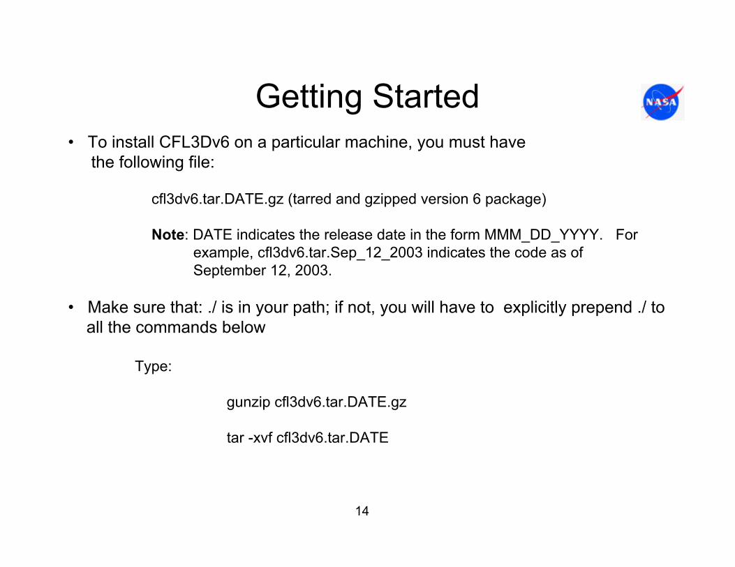
Getting Started• To install CFL3Dv6 on a particular machine, you must have
the following file:
cfl3dv6.tar.DATE.gz (tarred and gzipped version 6 package)
Note: DATE indicates the release date in the form MMM_DD_YYYY. Forexample, cfl3dv6.tar.Sep_12_2003 indicates the code as of September 12, 2003.
• Make sure that: ./ is in your path; if not, you will have to explicitly prepend ./ to all the commands below
Type:
gunzip cfl3dv6.tar.DATE.gz
tar -xvf cfl3dv6.tar.DATE

15
You should end up with the following directory structure:
CFL3DV6
SOURCE BUILD HEADER
Within the source directory:SOURCE
CFL3D PRECFL3D RONNIE MAGGIE SPLITTER TOOLS
DIST LIBS
Getting Started
16
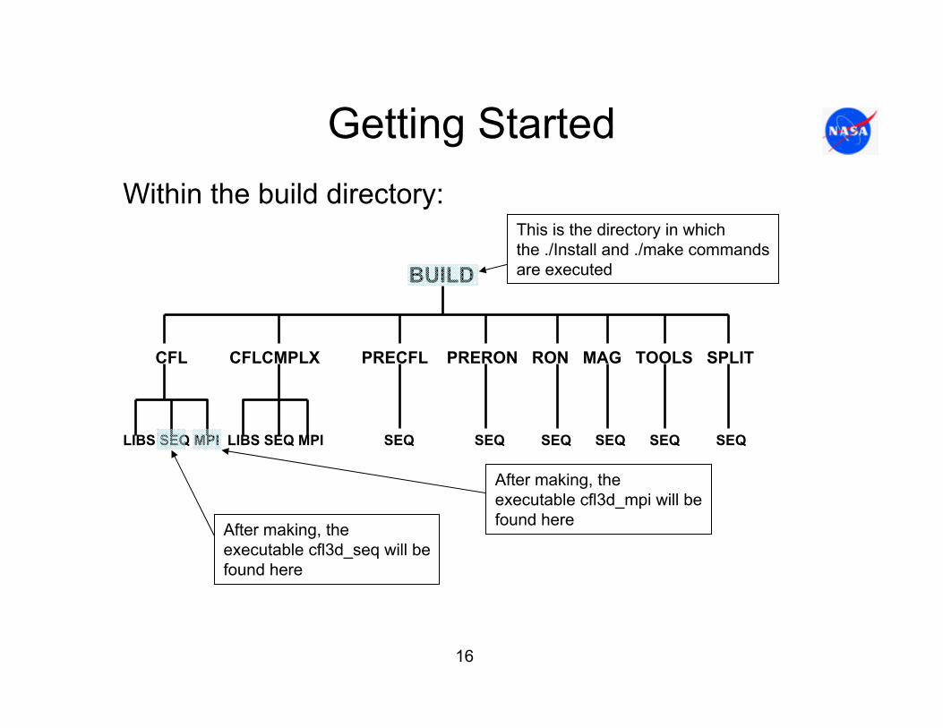
Getting StartedWithin the build directory:
BUILD
CFL CFLCMPLX PRECFL PRERON RON MAG TOOLS SPLIT
LIBS SEQ MPI LIBS SEQ MPI SEQ SEQ SEQ SEQ SEQ SEQ
This is the directory in whichthe ./Install and ./make commandsare executed
After making, the executable cfl3d_seq will befound here
After making, theexecutable cfl3d_mpi will befound here

17
Getting Started
– In the subdirectory build, type:
Install [options] or ./Install [options]
Where [options] may be blank or one or more of the following:
-no_opt• create executables with little optimization but fast compilation
-single • create single precision executables
-noredirect• disallow redirected input file; needed only for SP2 and sometimes on Linux with MPI
-mpichdir=dir1• use MPICH on a workstation cluster; dir1 is the directory where mpich is located - not used on MPP
machines -linux_compiler_flags=flag• sets up to compile using special compiler flags for use on Linux operating systems only; flag is
currently Intel, PG, Lahey, or Alpha (Intel is currently the default) Example: To use the Portland Group compiler MUST install with: ./Install -linux_compiler_flags=PG
-help • print out the Install options

18
Getting Started– Note: the directory paths for either the mpichdir or cgnsdir options
should be either absolute paths or paths relative to the installation directory; the use of ~ to denote a home directory is not allowed.
– If -no_opt is not specified, various compiler optimization levels are usedto speed execution but results in slower compilation.
– If -mpichdir=dir1 is not used, then it is assumed "native" MPI is available, and will use a default location for the necessary MPI libraries.
– If -single is not used, then double precision executables will be created at the make [ ] command.
– Once installation is complete, a makefile will automatically be created for the machine platform on which the code is installed.
– Go to the build directory. – By typing “make” you will see all the make options available.
19
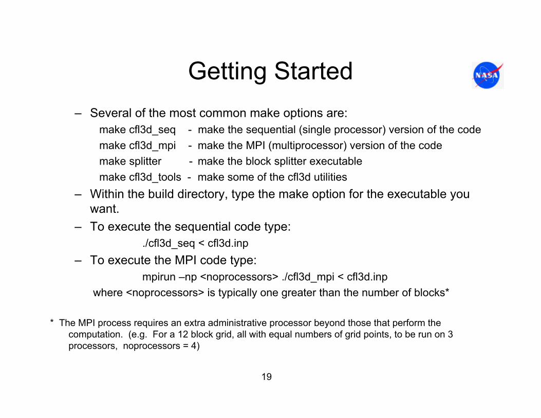
Getting Started– Several of the most common make options are:
make cfl3d_seq - make the sequential (single processor) version of the codemake cfl3d_mpi - make the MPI (multiprocessor) version of the codemake splitter - make the block splitter executablemake cfl3d_tools - make some of the cfl3d utilities
– Within the build directory, type the make option for the executable you want.
– To execute the sequential code type:./cfl3d_seq < cfl3d.inp
– To execute the MPI code type:mpirun –np <noprocessors> ./cfl3d_mpi < cfl3d.inp
where <noprocessors> is typically one greater than the number of blocks*
* The MPI process requires an extra administrative processor beyond those that perform the computation. (e.g. For a 12 block grid, all with equal numbers of grid points, to be run on 3 processors, noprocessors = 4)

20
Equations and DimensionsReference parameters
• The governing equations are the Euler or Navier-Stokes equations combined with a turbulence model for RANS computation
• The governing equations are non-dimensionalized based on the following parameters:
−−−−
∞
∞
∞
µ
ρ
~~~
~
a
LR Reference length used by the code (dimensional)
Free-stream density, mass/unit length cubed
Free-stream speed of sound, length/time
Free-stream molecular viscosity, mass/length-time

21
Equations and Dimensions
• Since there is no standard system of units for CFD models the non-dimensionalization in CFL3D removes the necessity of converting grids into units compatible with the code. The way in which the non-dimensionalization is accomplished will be presented later in this document.
• Note that the term free-stream is used in the non-dimensionalization. CFL3D was developed primarily asan external flow solver. It has the capability to perform computations for internal flows as well. Therefore a more general term reference state should probably be used, butthe term free-stream is used throughout the documentation.

22
Equations and DimensionsNon-dimensional variables
In CFL3D the non-dimensionalizations are performed as follows:
∞∞∞∞
∞
====
====
aww
avv
auu
Latt
Lzz
Lyy
Lxx
RRRR
~~
~~
~~
~~
~~~
~~
~~
~~
ρρρ
Velocities nondim-ensionalized by speed of sound
Time nondim-ensionalized by speed of soundand ref length
Non-dimensionalizing by speed of sound makes transonic the natural flow regime for CFL3D,although low speed and hypersonic flows can be computed, with modified input, as well.

23
Problem Formulation and SetupOverview
• There are five steps in problem formulation and setup for steady and unsteady computation:
- Condition definition- Grid generation- Block splitting (if necessary)- Blocking and boundary conditions- Input development
• Parameters that define a condition are:
- Mach number- Reynolds number- Ambient temperature- Grid orientation (angle of attack, side slip, etc…)
Input for these parameters will be discussed later. For the moment several ofthese parameters are required for the proper construction of the grid…

24
Problem Formulation and SetupGrid generation
Considerations that are important for generation of a grid:
• Reynolds number sets permissible ∆y+ at the surface.• For most turbulent computations typically want a y+ ~ 1
for first grid off the surface• For turbulent computations with wall function, typically want a
y+ ~ 50-100 for first grid off the surface• Setting ∆y+ requires an estimate of the wall shear stress prior to
computing
Note that:
where y is normal distance to surface, is wall shear stress, is densityand v is kinematic viscosity.
ρτ
νwyy =+
wτ ρ

25
Problem Formulation and SetupGrid generation
• After the first converged successful run with a coarse grid, y+ of the first grid can be checked. This value is found at the end of the cfl3d.out file. (See Y+ MAX, Y+ MIN and Y+AVG below)
YPLUS STATISTICS (endpts not included) - BLOCK 1 (GRID 1)
K=1 SURFACE:Y+ MAX JLOC ILOC Y+ MIN JLOC ILOC
0.535E+00 151 1 0.261E-01 217 1DN MAX JLOC ILOC DN MIN JLOC ILOC
0.152E-05 228 1 0.149E-05 219 1Y+ AVG Y+ STD DEV NY+ > 5 NPTS
0.264E+00 0.373E+00 0 199
YPLUS STATISTICS (endpts not included) - ALL GLOBAL BLOCKSY+ MAX ILOC JLOC KLOC BLOCK GRID
0.535E+00 1 151 1 1 1Y+ MIN ILOC JLOC KLOC BLOCK GRID
0.261E-01 1 217 1 1 1
etc…
26
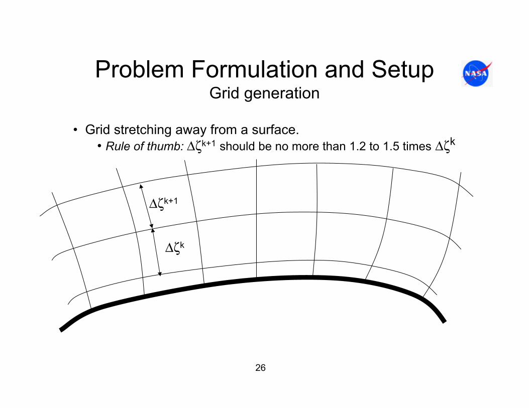
Problem Formulation and SetupGrid generation
• Grid stretching away from a surface. • Rule of thumb: ∆ζk+1 should be no more than 1.2 to 1.5 times ∆ζk
∆ζk+1
∆ζk

27
Problem Formulation and SetupGrid generation
• Outer extent of grid• Rule of thumb: The outer boundary of the grid should be at least
15 body lengths away (3D) and at least 20 body lengths away (2D). This is not a hard and fast rule and there are some notable exceptions. Note that the grid below would not be considered a fully acceptable grid.

28
Problem Formulation and SetupGrid generation
• Grid quality• Grid metric smoothness. CFL3D assesses the size of local
variations in grid metrics. Warnings are printed to the cfl3d.out file. Any messages of the following form indicate a problem with the grid:
FATAL si grid normal direction change near j,k,i,i+1= 23 5 164 165... suspect bad grid
FATAL sj grid normal direction change near j,k,i,i+1= 23 5 164 165... suspect bad grid
Etc… Or
WARNING: Dramatic si grid norm direction change (>120deg) WARNING: Dramatic sj grid norm direction change (>120deg)
Etc…

29
Problem Formulation and SetupGrid generation
• Grid quality (...continued)• Negative grid volumes. CFL3D checks whether there are
negative volumes in the grid. Under normal operating proceduresthe code will exit with an error message in the cfl3d.error file.*
• Grid clustering to resolve flow gradients• Resolving a wake. Although angle of attack is specified in the
input, it does result in the possibility of flow separation and wing stall and resulting wake. The wake may need grid clustering.
• Resolving a shock or curvature effect. Mach number effects such as a shock or surface curvature may result in gradients that require resolving.
• These steps must be performed prior to running CFL3D.
* There is a keyword option that allows computing to continue with negative volumes. This option will be discussed later in the course under “Keyword Input”.

30
Problem Formulation and SetupGrid generation
• Grid file format• The grid file format must be unformatted• Two grid data formats are possible, plot3d and cfl3d. These
formats are presented in the CFL3D version 5.0 manual.• If CFL3D is compiled in double precision, the grid file must be
written as double precision real• Example of multi-platform issue: If a Linux compiler is used to
compile CFL3D to read an SGI unformatted grid file, the grid file must be generated with the same compile options
Example: Suppose the code ‘hygrid’ is used to generate the unformatted grid file. On a Linux based PC platform using the Portland Groupcompiler, the compile option –byteswapio swaps bytes from big-endian to little-endian for input compatibility with a Sun or SGI system. This compiler option will allow CFL3D to read the grid file created either on the PC cluster or on an SGI machine.

31
Problem Formulation and SetupGrid generation
CFL3D requires that the right-hand rule be observed in both the x,y,z orientation and the i,j,k index directions. Also, i,j and k do not have to be in the x,y and z directions. Any permutation is valid as long as the right-hand rule is upheld. Caveat: When using turbulence models there are direction preferences as will be discussed.
k
ij
k
i
j
32
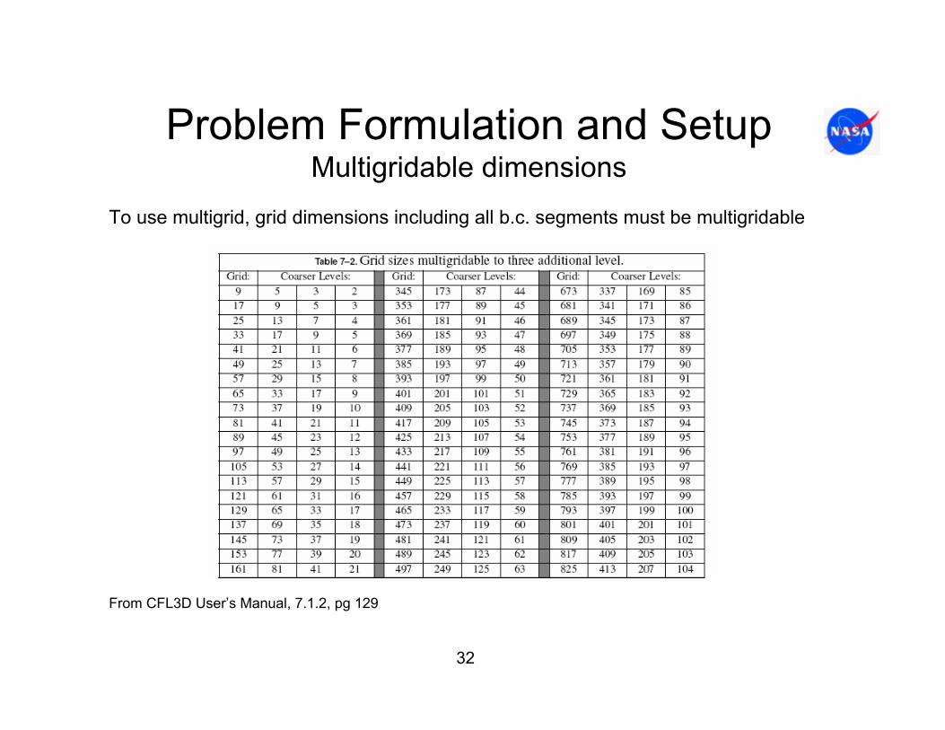
Problem Formulation and SetupMultigridable dimensions
From CFL3D User’s Manual, 7.1.2, pg 129
To use multigrid, grid dimensions including all b.c. segments must be multigridable
33
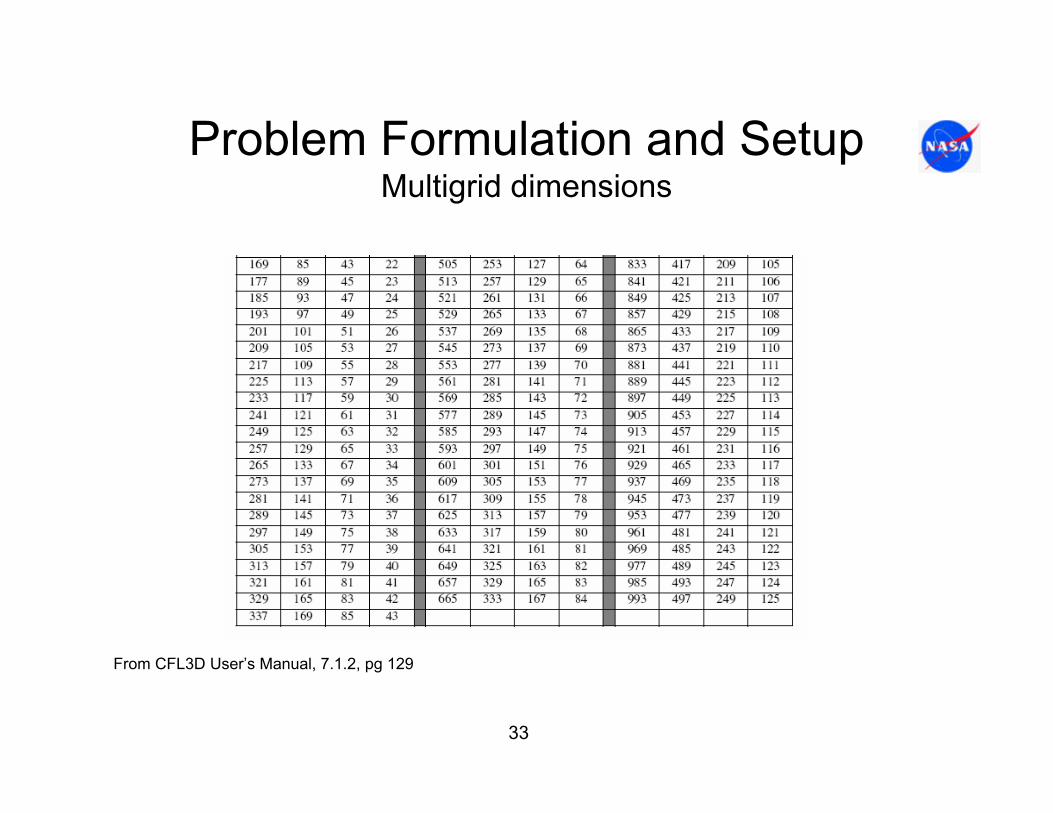
Problem Formulation and SetupMultigrid dimensions
From CFL3D User’s Manual, 7.1.2, pg 129

34
Problem Formulation and SetupBlocking and boundary conditions
Blocking and boundary conditions are specified at the following boundaries:
i0 (i=1) and idimj0 (j=1) and jdimk0 (k=1) and kdim
where idim, jdim and kdim are the block dimensions in the ijk-directions. Blocking and boundary condition data can be composed of multiplesegments but the combined segments must span each of the six block faces. Note that to perform multigrid computations, the boundary and blocking segments must be multigridable integers.

35
Problem Formulation and SetupBlocking and boundary conditions
Example of possible blocking or boundary condition segments on the k0 face. Suppose that part of the k0 face below represents the surface of a wing.
i=1 i=5
j=1
j=4
Blockingsegment
Solid surface boundarycondition segment
36
Problem Formulation and SetupBlocking and boundary conditions
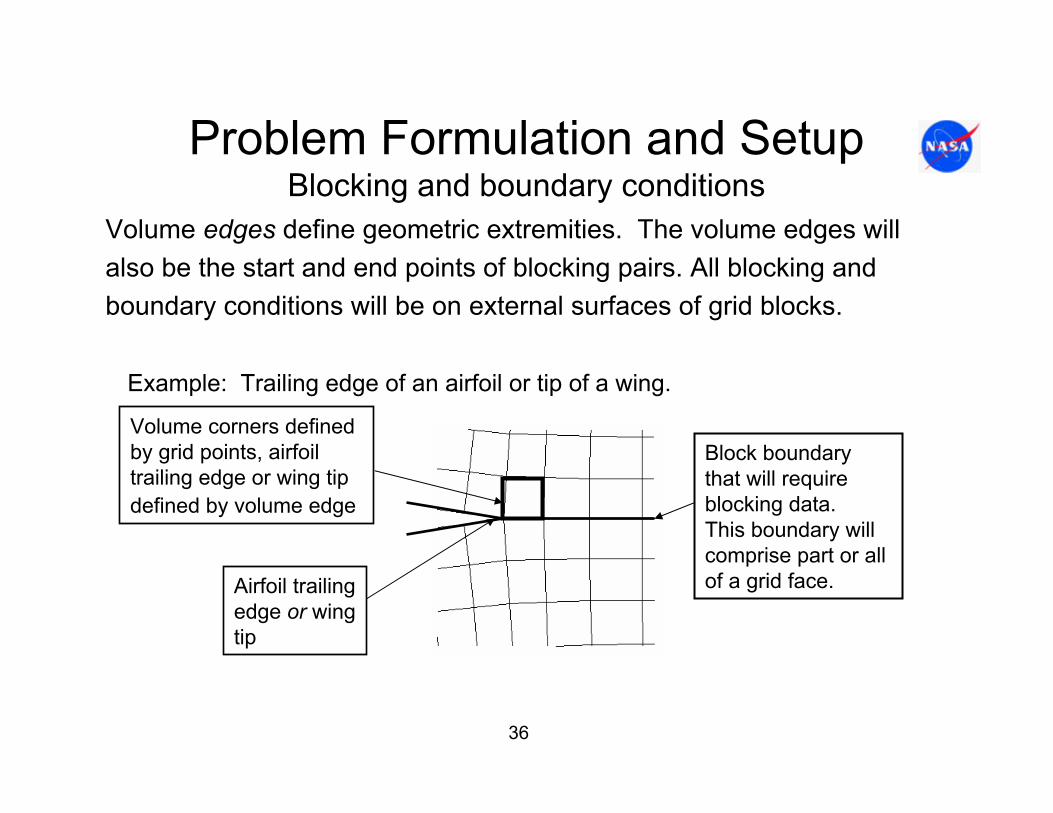
Volume edges define geometric extremities. The volume edges will also be the start and end points of blocking pairs. All blocking and boundary conditions will be on external surfaces of grid blocks.
Example: Trailing edge of an airfoil or tip of a wing.
Volume corners defined by grid points, airfoil trailing edge or wing tipdefined by volume edge
Airfoil trailingedge or wingtip
Block boundarythat will requireblocking data. This boundary willcomprise part or all of a grid face.

37
Problem Formulation and SetupBlocking and boundary conditions
Blocking defines the start and ending indices of 1-1 interfaces between one or more corresponding grid blocks.
Consider the example of a 2D airfoil using a single block C-grid with dimension 2x273x93. CFL3D is a finite volume code and therefore requires 2 grid points in the span-wise direction (always i-dir for a 2D grid). Note that the arrows in the right hand figurebelow denotes the end of a blocking segment. The meaning of this statement will be made clear in the following pages.
j=1j=37(t.e.)
j=237(t.e.) j=273
j=1
j=273
k=1
k=93
38
Problem Formulation and SetupBlocking and boundary conditions
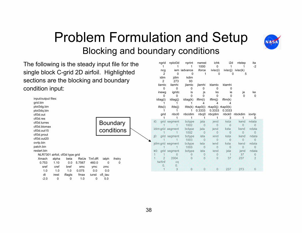
The following is the steady input file for the single block C-grid 2D airfoil. Highlighted sections are the blocking and boundary condition input:
input/output files:grid.binplot3dg.binplot3dq.bincfl3d.outcfl3d.rescfl3d.turrescfl3d.blomaxcfl3d.out15cfl3d.proutcfl3d.out20ovrlp.binpatch.binrestart.bin
NLR7301 airfoil, cfl3d type gridXmach alpha beta ReUe Tinf,dR ialph ihstry
0.753 1.10 0.0 5.7567 460.0 0 0sref cref bref xmc ymc zmc1.0 1.0 1.0 0.075 0.0 0.0dt irest iflagts fmax iunst cfl_tau
-2.0 0 0 1.0 0 5.0
ngrid nplot3d nprint nwrest ichk i2d ntstep ita1 1 1 1000 0 1 1 -2
ncg iem iadvance iforce ivisc(i) ivisc(j) ivisc(k)2 0 0 1 0 0 5
idim jdim kdim2 273 93
ilamlo ilamhi jlamlo jlamhi klamlo klamhi0 0 0 0 0 0
inewg igridc is js ks ie je ke0 0 0 0 0 0 0 0
idiag(i) idiag(j) idiag(k) iflim(i) iflim(j) iflim(k)1 1 1 4 4 4
ifds(i) ifds(j) ifds(k) rkap0(i) rkap0(j) rkap0(k)1 1 1 0.3333 0.3333 0.3333
grid nbci0 nbcidim nbcj0 nbcjdim nbck0 nbckdim iovrlp1 1 1 1 1 3 1 0
i0: grid segment bctype jsta jend ksta kend ndata1 1 1002 0 0 0 0 0
idim:grid segment bctype jsta jend ksta kend ndata1 1 1002 0 0 0 0 0
j0: grid segment bctype ista iend ksta kend ndata1 1 1003 0 0 0 0 0
jdim:grid segment bctype ista iend ksta kend ndata1 1 1003 0 0 0 0 0
k0: grid segment bctype ista iend jsta jend ndata1 1 0 0 0 0 1 37 01 2 2004 0 0 0 37 237 2
tw/tinf cq0. 0.1 3 0 0 0 237 273 0
Boundary conditions

39
Problem Formulation and SetupBlocking and boundary conditions
kdim:grid segment bctype ista iend jsta jend ndata1 1 1003 0 0 0 0 0
mseq mgflag iconsf mtt ngam1 1 0 0 2
issc epsssc(1) epsssc(2) epsssc(3) issr epsssr(1) epsssr(2) epsssr(3)0 0.3 0.3 0.3 0 0.3 0.3 0.3
ncyc mglevg nemgl nitfo2000 3 0 0
mit1 mit2 mit3 mit4 mit5 ... 1 1 1
1-1 blocking data:nbli
1number grid ista jsta ksta iend jend kend isva1 isva2
1 1 1 1 1 2 37 1 1 2number grid ista jsta ksta iend jend kend isva1 isva2
1 1 1 273 1 2 237 1 1 2patch interface data:
ninter0
plot3d output:grid iptyp ista iend iinc jsta jend jinc ksta kend kinc
1 0 1 1 1 1 999 1 1 999 1movie
0print out:
grid iptyp ista iend iinc jsta jend jinc ksta kend kinc1 0 1 1 1 1 999 1 1 999 1
control surfacesncs
0grid ista iend jsta jend ksta kend iwall inorm
Blockingdata

40
Problem Formulation and SetupBlocking and boundary conditions
For this example, format of the blocking data in the input file:
1-1 blocking data:nbli
1number grid ista jsta ksta iend jend kend isva1 isva2
1 1 1 1 1 2 37 1 1 2number grid ista jsta ksta iend jend kend isva1 isva2
1 1 1 273 1 2 237 1 1 2
Number of the blocking data line
Number of the block (in the present example there is only 1 block)
Number of lines of blocking dataNo. of linesin each datamust equal nbli
Note: The text cards must be present, but the text within those linesis arbitrary, and is for user information only. All lines with data are in free field format throughout the input file.
41
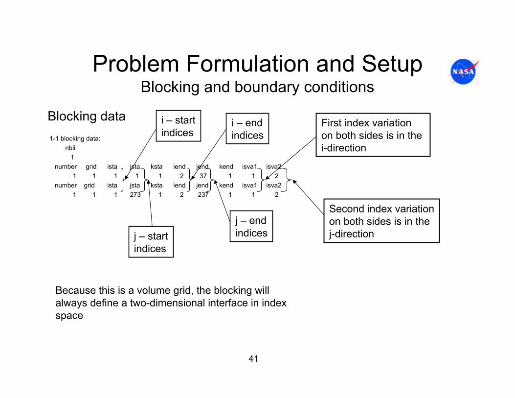
Problem Formulation and SetupBlocking and boundary conditions
Blocking data1-1 blocking data:
nbli1
number grid ista jsta ksta iend jend kend isva1 isva21 1 1 1 1 2 37 1 1 2
number grid ista jsta ksta iend jend kend isva1 isva21 1 1 273 1 2 237 1 1 2
j – startindices
j – endindices
i – startindices
i – endindices
Because this is a volume grid, the blocking will always define a two-dimensional interface in index space
First index variationon both sides is in the i-direction
Second index variationon both sides is in the j-direction

42
Problem Formulation and SetupBlocking and boundary conditions
Consider a second example of a 2D airfoil using two blocks to compose aC-grid. Block 1 has dimensions 2x93x5. Block 2 has dimensions 2x269x93.Note again that the arrows in the right hand figure below denotes the end of a blocking segment. This fact is made clear by the following page.
j=1j=33(t.e.)
j=233(t.e.)
j=269
Block boundaryk=1k=5
j=265
j=265
Block 1
Block 2

43
Problem Formulation and SetupBlocking and boundary conditions
Blocking data
1-1 blocking data:
nbli3
number grid ista jsta ksta iend jend kend isva1 isva21 1 1 1 1 2 1 5 1 32 2 1 1 1 2 33 1 1 23 1 1 1 1 2 97 1 1 2
number grid ista jsta ksta iend jend kend isva1 isva21 2 1 269 1 2 265 1 1 22 2 1 265 1 2 233 1 1 23 2 1 1 1 2 1 97 1 3
3 blocking datasets now
k-index of block 1 nowvaries with the j-index ofblock 2
A new blocking boundary appears that previously didnot exist
44
Problem Formulation and SetupBlocking and boundary conditions
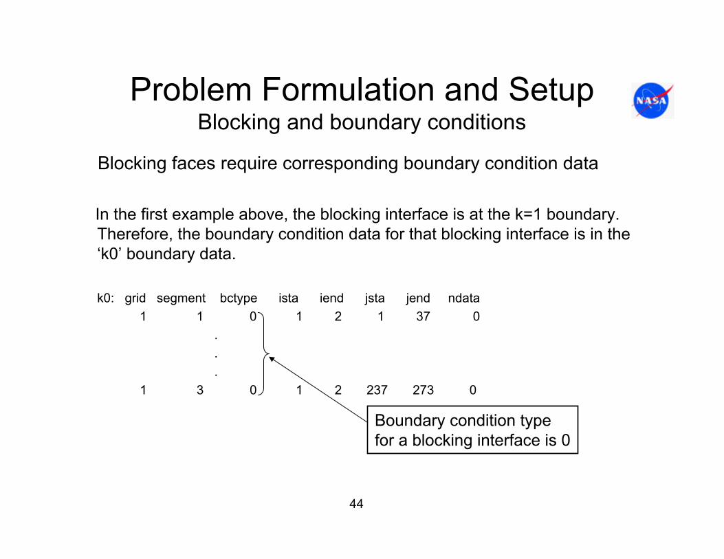
Blocking faces require corresponding boundary condition data
In the first example above, the blocking interface is at the k=1 boundary. Therefore, the boundary condition data for that blocking interface is in the ‘k0’ boundary data.
k0: grid segment bctype ista iend jsta jend ndata1 1 0 1 2 1 37 0
.
.
.1 3 0 1 2 237 273 0
Boundary condition typefor a blocking interface is 0

45
Problem Formulation and SetupBlocking and boundary conditions
CFL3D will stop if the number of grid points across a blocking interfaces does not match.
Suppose the following blocking data had been specified for example 1 above:
number grid ista jsta ksta iend jend kend isva1 isva21 1 1 1 1 2 35 1 1 2
number grid ista jsta ksta iend jend kend isva1 isva21 1 1 273 1 2 237 1 1 2
Execution will terminate with the following error message at the end of the file ‘precfl3d.out’:
.
.the limits of ind2 are not the same for both sides for 1:1 plane 1
Erroneousjend value

46
Problem Formulation and SetupBlocking and boundary conditions
CFL3D also checks the input connection data by computing the geometric mismatch between both sides of the interface. A true 1-1 interface will have zero (machine zero) mismatch. Any mismatches larger than ε (where ε is the larger of 10-9 or 10x(machine zero)) will cause a warning message.
Example of the output in ‘cfl3d.out’:
j= 1 1-1 blocking type 0 i= 1, 31 k=137, 69connects to j = 1 of block 2blocking check....geometric mismatch = 0.2166272E-03

47
Problem Formulation and SetupBlocking and boundary conditions
Example of possible boundary condition segments on the k0 face. Suppose that the k0 face below represents the surface of a wing.
i=1 i=5j=1
j=4

48
Problem Formulation and SetupBlocking and boundary conditions
At the unshaded cells, it is desired to apply a heated wall boundary condition, while at the shaded cells it is desired to apply an adiabatic wall boundary condition. One way to accomplish this objective is to divide the boundary into the segments shown. The CFL3D input file would have input that looks like this:
k0: grid segment bctype ista iend jsta jend ndata1 1 2004 1 5 1 2 2
tw/tinf cq1.60000 0.00000
1 2 2004 1 3 2 4 2tw/tinf cq
1.60000 0.00000 1 3 2004 3 5 2 4 2
tw/tinf cq0.00000 0.00000
Note that for segment 1, for instance, the grid points i = 1 to 5, j = 1 to 2 define the boundary of the cells at which the condition type is to be applied.
j=1
j=4
i=1 i=5
Segment 1
Segment 2 Segment 3

49
Problem Formulation and SetupBlocking and boundary conditions
Setting ista = iend = 0 and/or jsta = jend = 0 is a shorthand way of specifying the entire range. In other words, an alternate boundary condition input with identical outcome is:
k0: grid segment bctype ista iend jsta jend ndata1 1 2004 0 0 1 2 2
tw/tinf cq1.60000 0.00000
1 2 2004 1 3 2 4 2tw/tinf cq
1.60000 0.00000 1 3 2004 3 5 2 4 2
tw/tinf cq0.00000 0.00000
j=1
j=4
i=1 i=5
Segment 1
Segment 2 Segment 3

50
Problem Formulation and SetupBlocking and boundary conditions
The following 1000 series boundary conditions are available:
bctype boundary condition1000 free stream1001 general symmetry plane1002 extrapolation1003 inflow/outflow1005 inviscid surface1006 inviscid surface (using normal momentum)1008 tunnel inflow1011 singular axis – half-plane symmetry1012 singular axis – full plane1013 singular axis – partial plane
Refer to the Version 5.0 Manual and Version 6.0 web page for more information on theseboundary conditions

51
Problem Formulation and SetupBlocking and boundary conditions
The following 2000 series boundary conditions are available:
bctype boundary condition2002 specified pressure ratio2003 inflow with specified total conditions2004 no-slip wall2005 periodic in space2006 set pressure to satisfy the radial equilibrium equation2007 set all primitive variables
Refer to the Version 5.0 Manual and Version 6.0 web page for more information on theseboundary conditions

52
Problem Formulation and SetupBlocking and boundary conditions
The following 2000 series boundary conditions are available:
bctype boundary condition2008 user specifies density and velocity components,
pressure extrapolated from interior2009 sets total pressure and total temperature. Inflow pressure
extrapolated from interior2014 user specifies transpiration through the boundary2018 user specifies temperature and momentum components,
pressure extrapolated from interior2028 user specifies frequency and maximum momentum
components, density and pressure extrapolated 2102 pressure ratio specified as a sinusoidal function of time
Refer to the Version 5.0 Manual and Version 6.0 web page for more information on theseboundary conditions

53
Problem Formulation and SetupBlocking and boundary conditions
Boundary condition 1000 - Free stream. Extrapolation points just outside the boundary are set to initial free stream values, which are:
where is density, u,v,w are the x,y,z components of velocity, p is pressure, a is speed of sound and is ratio of specific heats. M is Mach number, is the angleof attack and is the side slip angle.
γρβα
ββα
ρ
/
cossinsin
coscos0.1
2initialinitialinitial
initial
initial
initial
initial
ap
MwMv
Mu
=
=−=
==
∞
∞
∞
ργ
βα

54
Problem Formulation and SetupBlocking and boundary conditions
Boundary condition 1001 - General symmetry plane. Suppose we wish to simulate a 3D wing using the half wing shown. If only one type of maneuver isperformed (i.e. with aircraft maneuver symmetry in the x-y plane, x-z plane ory-z plane only) the symmetry plane boundary condition can be used.
General symmetry plane
55
Problem Formulation and SetupBlocking and boundary conditions
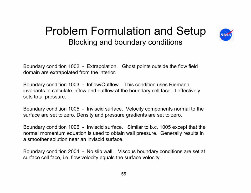
Boundary condition 1002 - Extrapolation. Ghost points outside the flow field domain are extrapolated from the interior.
Boundary condition 1003 - Inflow/Outflow. This condition uses Riemann invariants to calculate inflow and outflow at the boundary cell face. It effectivelysets total pressure.
Boundary condition 1005 - Inviscid surface. Velocity components normal to the surface are set to zero. Density and pressure gradients are set to zero.
Boundary condition 1006 - Inviscid surface. Similar to b.c. 1005 except that the normal momentum equation is used to obtain wall pressure. Generally results in a smoother solution near an inviscid surface.
Boundary condition 2004 - No slip wall. Viscous boundary conditions are set at surface cell face, i.e. flow velocity equals the surface velocity.
56
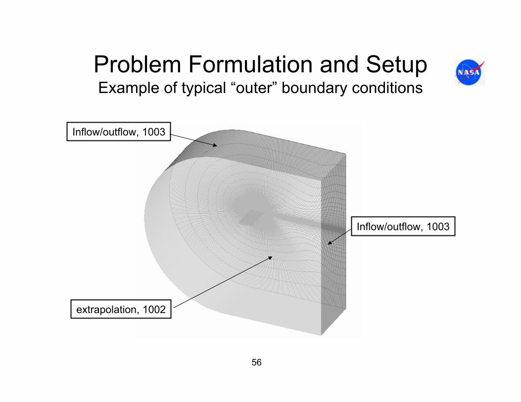
Problem Formulation and SetupExample of typical “outer” boundary conditions
Inflow/outflow, 1003
Inflow/outflow, 1003
extrapolation, 1002
57
Problem Formulation and SetupBlocking and boundary conditions
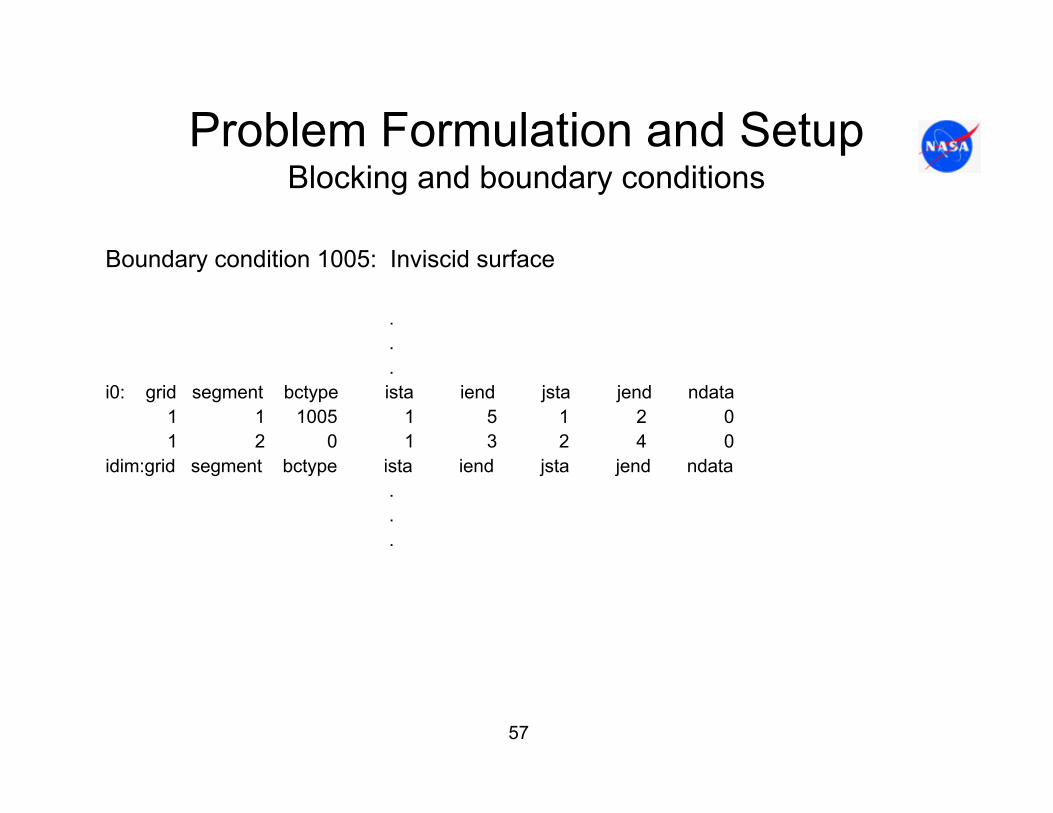
Boundary condition 1005: Inviscid surface
.
.
.i0: grid segment bctype ista iend jsta jend ndata
1 1 1005 1 5 1 2 01 2 0 1 3 2 4 0
idim:grid segment bctype ista iend jsta jend ndata...

58
Problem Formulation and SetupBlocking and boundary conditions
Note that the b.c. 1005 has no auxiliary data, while the b.c. 2004 has two additional lines
.
.k0: grid segment bctype ista iend jsta jend ndata
1 1 1005 1 5 1 2 0..
…versus…..
k0: grid segment bctype ista iend jsta jend ndata1 1 2004 1 5 1 2 2
tw/tinf cq
1.60000 0.00000
Specifies noadditional data entries
Specifies twoadditional auxiliarydata entries

59
Problem Formulation and SetupBlocking and boundary conditions
• Series 1000 boundary conditions require no auxiliary data• Number of auxiliary data entries for series 2000 boundary conditions
are shown below
b.c. type No. of auxiliarydata
2002 12003 52004 22005 52006 42007 5*2008 4*2009 4*2014 32016 72018 4*2028 4*2102 4
* Means turbulence data can also be specified, adding either 1 or 2 additional aux. data inputs
See the CFL3D version 5.0 manual and CFL3D Version 6 web page for discussion of these boundary conditions

60
Problem Formulation and SetupBlocking and boundary conditions
Example of a boundary condition with 5 auxiliary data entries: 2003 -“Engine inflow”, inflow with specified total conditions:
.
.k0: grid segment bctype ista iend jsta jend ndata
1 1 2003 1 5 1 2 5Mach Pt/Pinf Tt/Tinf Alphae Betae0.30 4.000 1.1755 0.0 0.0
.
.

61
Problem Formulation and SetupBlocking and boundary conditions
.
.
.grid nbci0 nbcidim nbcj0 nbcjdim nbck0 nbckdim iovrlp
1 1 1 1 1 3 1 0i0: grid segment bctype jsta jend ksta kend ndata
1 1 1002 0 0 0 0 0idim: grid segment bctype jsta jend ksta kend ndata
1 1 1002 0 0 0 0 0j0: grid segment bctype ista iend ksta kend ndata
1 1 1003 0 0 0 0 0jdim: grid segment bctype ista iend ksta kend ndata
1 1 1003 0 0 0 0 0k0: grid segment bctype ista iend jsta jend ndata
1 1 0 0 0 1 37 01 2 2004 0 0 37 237 2
tw/tinf cq0. 0. 1 3 0 0 0 237 273 0
kdim: grid segment bctype ista iend jsta jend ndata1 1 1003 0 0 0 0 0
.
.
.1-1 blocking data:
nbli1
number grid ista jsta ksta iend jend kend isva1 isva21 1 1 1 1 2 37 1 1 2
number grid ista jsta ksta iend jend kend isva1 isva21 1 1 273 1 2 237 1 1 2
.
.
Boundary conditiondata
Blocking data
Input data so far for the 2D airfoil using a single block C-grid
i-boundary data
j-boundary data
k-boundary data
Number of k0 segments
62
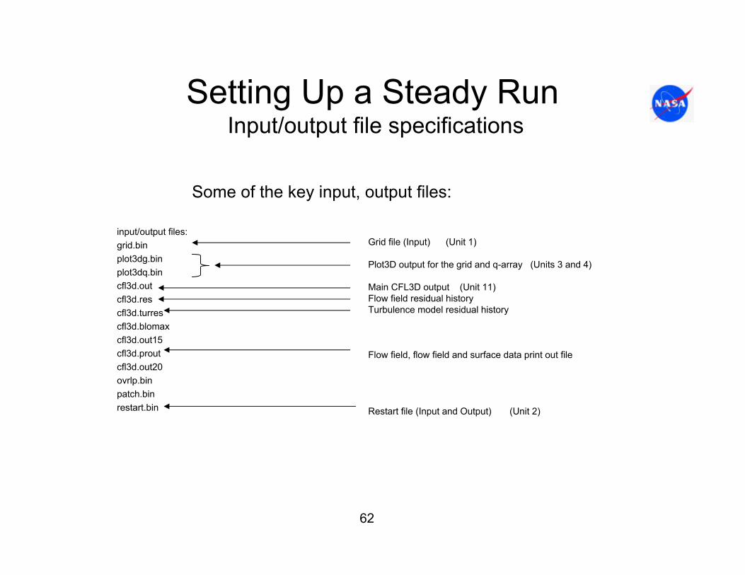
Setting Up a Steady RunInput/output file specifications
input/output files:grid.binplot3dg.binplot3dq.bincfl3d.outcfl3d.rescfl3d.turrescfl3d.blomaxcfl3d.out15cfl3d.proutcfl3d.out20ovrlp.binpatch.binrestart.bin
Grid file (Input) (Unit 1)
Plot3D output for the grid and q-array (Units 3 and 4)
Main CFL3D output (Unit 11)Flow field residual historyTurbulence model residual history
Flow field, flow field and surface data print out file
Restart file (Input and Output) (Unit 2)
Some of the key input, output files:

63
Setting Up a Steady RunInput/output file specifications
• These names can be changed by the user. • Input/output redirects are permitted. (e.g. ../../grid.bin or
./cflout/cfl3d.out)• Additional files are printed out not contained in this list. (e.g.
precfl3d.out, precfl3d.error, cfl3d.error, cfl3d.subit_res and cfl3d.subit_turres) These files cannot be renamed or redirected
• The restart file name that is read at the start of the computation is the same name used for output at the end. Scripting that saves restart files to another name will be required if the user wishes to save the input restart.
64
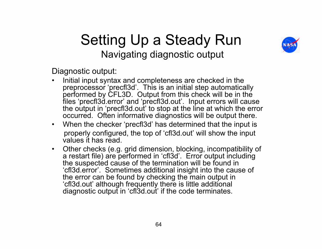
Setting Up a Steady RunNavigating diagnostic output
Diagnostic output:• Initial input syntax and completeness are checked in the
preprocessor ‘precfl3d’. This is an initial step automatically performed by CFL3D. Output from this check will be in the files ‘precfl3d.error’ and ‘precfl3d.out’. Input errors will cause the output in ‘precfl3d.out’ to stop at the line at which the error occurred. Often informative diagnostics will be output there.
• When the checker ‘precfl3d’ has determined that the input isproperly configured, the top of ‘cfl3d.out’ will show the input values it has read.
• Other checks (e.g. grid dimension, blocking, incompatibility of a restart file) are performed in ‘cfl3d’. Error output including the suspected cause of the termination will be found in ‘cfl3d.error’. Sometimes additional insight into the cause of the error can be found by checking the main output in ‘cfl3d.out’ although frequently there is little additional diagnostic output in ‘cfl3d.out’ if the code terminates.
65
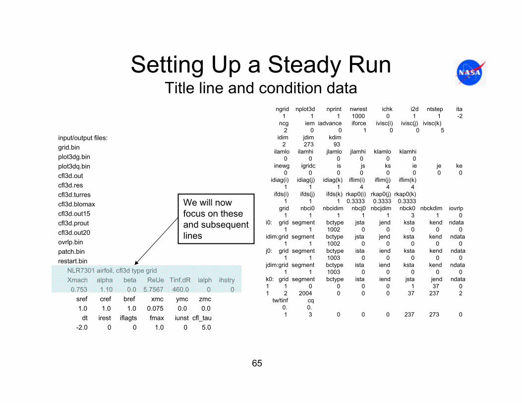
Setting Up a Steady RunTitle line and condition data
input/output files:grid.binplot3dg.binplot3dq.bincfl3d.outcfl3d.rescfl3d.turrescfl3d.blomaxcfl3d.out15cfl3d.proutcfl3d.out20ovrlp.binpatch.binrestart.bin
NLR7301 airfoil, cfl3d type gridXmach alpha beta ReUe Tinf,dR ialph ihstry0.753 1.10 0.0 5.7567 460.0 0 0
sref cref bref xmc ymc zmc1.0 1.0 1.0 0.075 0.0 0.0
dt irest iflagts fmax iunst cfl_tau-2.0 0 0 1.0 0 5.0
ngrid nplot3d nprint nwrest ichk i2d ntstep ita1 1 1 1000 0 1 1 -2
ncg iem iadvance iforce ivisc(i) ivisc(j) ivisc(k)2 0 0 1 0 0 5
idim jdim kdim2 273 93
ilamlo ilamhi jlamlo jlamhi klamlo klamhi0 0 0 0 0 0
inewg igridc is js ks ie je ke0 0 0 0 0 0 0 0
idiag(i) idiag(j) idiag(k) iflim(i) iflim(j) iflim(k)1 1 1 4 4 4
ifds(i) ifds(j) ifds(k) rkap0(i) rkap0(j) rkap0(k)1 1 1 0.3333 0.3333 0.3333
grid nbci0 nbcidim nbcj0 nbcjdim nbck0 nbckdim iovrlp1 1 1 1 1 3 1 0
i0: grid segment bctype jsta jend ksta kend ndata1 1 1002 0 0 0 0 0
idim:grid segment bctype jsta jend ksta kend ndata1 1 1002 0 0 0 0 0
j0: grid segment bctype ista iend ksta kend ndata1 1 1003 0 0 0 0 0
jdim:grid segment bctype ista iend ksta kend ndata1 1 1003 0 0 0 0 0
k0: grid segment bctype ista iend jsta jend ndata1 1 0 0 0 0 1 37 01 2 2004 0 0 0 37 237 2
tw/tinf cq0. 0.1 3 0 0 0 237 273 0
We will nowfocus on theseand subsequentlines

66
Setting Up a Steady RunTitle line and condition data
NLR7301 airfoil, cfl3d type C-gridXmach alpha beta ReUe Tinf,dR ialph ihstry0.753 1.10 0.0 5.7567 460.0 0 0
Condition title line
Condition dataline
Free-stream temperature, degrees Rankine
ialph – indicator to determine whether angle of attack is measured in the x-z plane or the x-y plane
ihstry – determines which variables are to be tracked for convergence history. Default is Cl, Cd, Cy (or Cz), Cm.
Input of ReUe (Reynolds number) requires some additional explanation….
Angle of attack, Deg.
Sideslip, Deg.

67
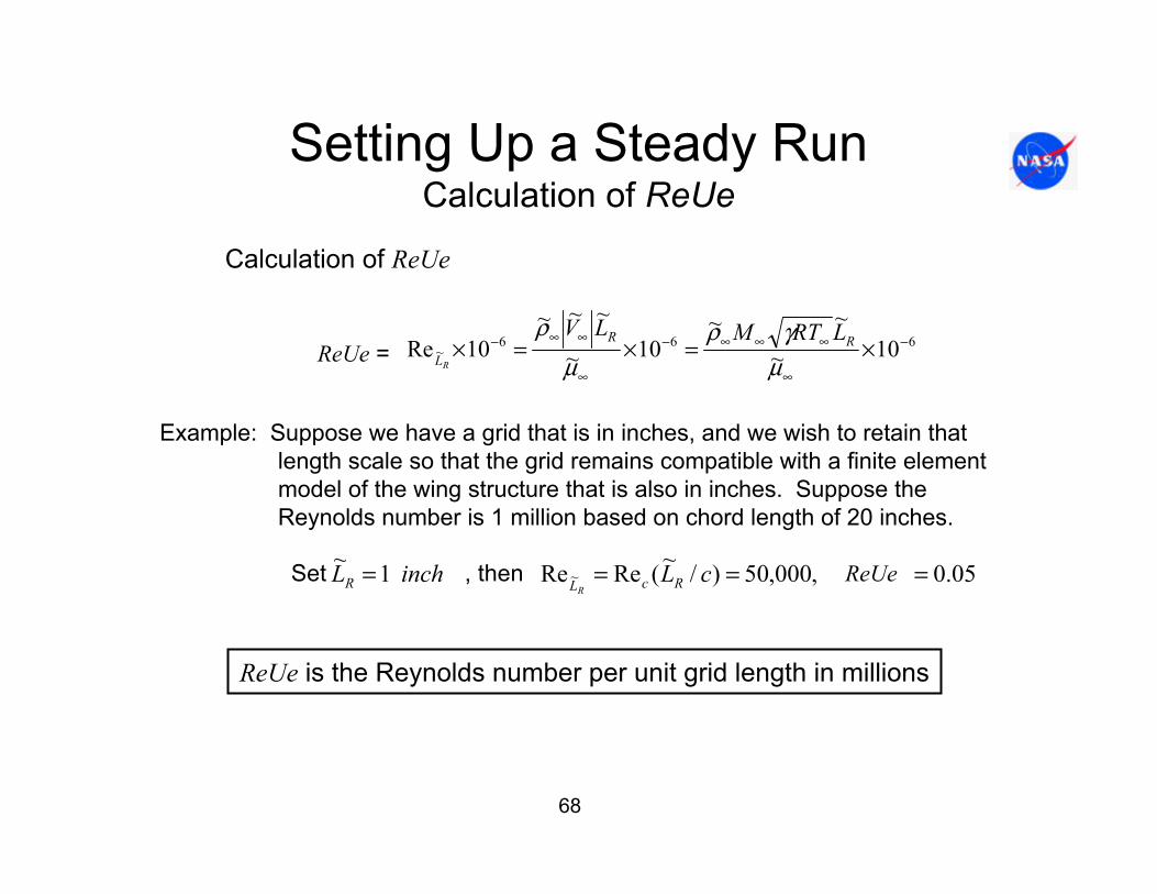
Setting Up a Steady RunCalculation of ReUe
Recall the nondimensionalizations:
∞∞∞∞
∞
====
====
aww
avv
auu
Latt
Lzz
Lyy
Lxx
RRRR
~~
~~
~~
~~
~~~
~~
~~
~~
ρρρ
Reference length
Reynolds number based on reference length:
∞
∞∞=µ
ρ~
~~~Re ~
R
L
LVR
68
Setting Up a Steady RunCalculation of ReUe
Calculation of ReUe
ReUe =
Example: Suppose we have a grid that is in inches, and we wish to retain that length scale so that the grid remains compatible with a finite elementmodel of the wing structure that is also in inches. Suppose the Reynolds number is 1 million based on chord length of 20 inches.
Set , then ReUe
ReUe is the Reynolds number per unit grid length in millions
05.0,000,50)/~(ReRe1~~ ==== cLinchL RcLR R
666~ 10~
~~10~
~~~10Re −
∞
∞∞∞−
∞
∞∞− ×=×=×µ
γρµ
ρRR
L
LRTMLVR
69
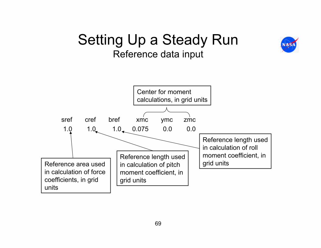
Setting Up a Steady RunReference data input
sref cref bref xmc ymc zmc1.0 1.0 1.0 0.075 0.0 0.0
Reference area usedin calculation of force coefficients, in grid units
Reference length usedin calculation of pitchmoment coefficient, in grid units
Reference length usedin calculation of rollmoment coefficient, in grid units
Center for momentcalculations, in grid units

70
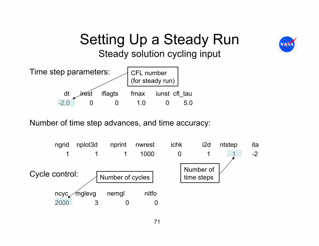
Setting Up a Steady RunSteady solution cycling input
input/output files:grid.binplot3dg.binplot3dq.bincfl3d.outcfl3d.rescfl3d.turrescfl3d.blomaxcfl3d.out15cfl3d.proutcfl3d.out20ovrlp.binpatch.binrestart.bin
NLR7301 airfoil, cfl3d type gridXmach alpha beta ReUe Tinf,dR ialph ihstry
0.753 1.10 0.0 5.7567 460.0 0 0sref cref bref xmc ymc zmc1.0 1.0 1.0 0.075 0.0 0.0dt irest iflagts fmax iunst cfl_tau
-2.0 0 0 1.0 0 5.0
ngrid nplot3d nprint nwrest ichk i2d ntstep ita1 1 1 1000 0 1 1 -2
ncg iem iadvance iforce ivisc(i) ivisc(j) ivisc(k)2 0 0 1 0 0 5
idim jdim kdim2 273 93
ilamlo ilamhi jlamlo jlamhi klamlo klamhi0 0 0 0 0 0
inewg igridc is js ks ie je ke0 0 0 0 0 0 0 0
idiag(i) idiag(j) idiag(k) iflim(i) iflim(j) iflim(k)1 1 1 4 4 4
ifds(i) ifds(j) ifds(k) rkap0(i) rkap0(j) rkap0(k)1 1 1 0.3333 0.3333 0.3333
.
.
.
mseq mgflag iconsf mtt ngam1 1 0 0 2
issc epsssc(1) epsssc(2) epsssc(3) issr epsssr(1) epsssr(2) epsssr(3)0 0.3 0.3 0.3 0 0.3 0.3 0.3
ncyc mglevg nemgl nitfo2000 3 0 0mit1 mit2 mit3 mit4 mit5 ...
1 1 1
We will now want to focus on these three lines
71
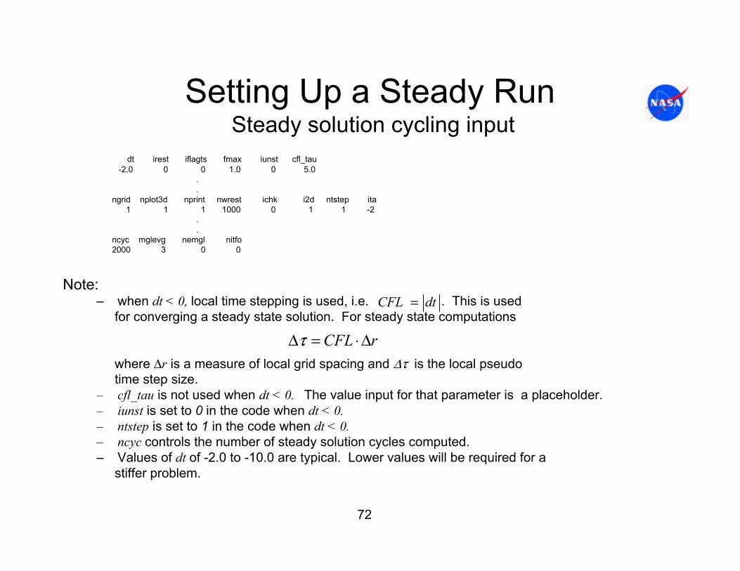
Setting Up a Steady RunSteady solution cycling input
Time step parameters:
dt irest iflagts fmax iunst cfl_tau-2.0 0 0 1.0 0 5.0
Number of time step advances, and time accuracy:
ngrid nplot3d nprint nwrest ichk i2d ntstep ita1 1 1 1000 0 1 1 -2
Cycle control:
ncyc mglevg nemgl nitfo2000 3 0 0
CFL number(for steady run)
Number of time stepsNumber of cycles
72
Setting Up a Steady RunSteady solution cycling input
dt irest iflagts fmax iunst cfl_tau-2.0 0 0 1.0 0 5.0
.
.ngrid nplot3d nprint nwrest ichk i2d ntstep ita
1 1 1 1000 0 1 1 -2..
ncyc mglevg nemgl nitfo2000 3 0 0
Note: – when dt < 0, local time stepping is used, i.e. . This is used
for converging a steady state solution. For steady state computations
where ∆r is a measure of local grid spacing and ∆τ is the local pseudo time step size.
– cfl_tau is not used when dt < 0. The value input for that parameter is a placeholder. – iunst is set to 0 in the code when dt < 0. – ntstep is set to 1 in the code when dt < 0. – ncyc controls the number of steady solution cycles computed.– Values of dt of -2.0 to -10.0 are typical. Lower values will be required for a
stiffer problem.
dtCFL =
rCFL ∆⋅=∆τ

73
Setting Up a Steady RunGrid sequencing
Grid sequencing can and should be used to accelerate convergence to asteady state solution. The following input sequences through three grid levels.
.
.ncg iem iadvance iforce ivisc(i) ivisc(j) ivisc(k)
2 0 0 1 0 0 5
.
.
.mseq mgflag iconsf mtt ngam
3 1 0 0 2issc epsssc(1) epsssc(2) epsssc(3) issr epsssr(1) epsssr(2) epsssr(3)
0 0.3 0.3 0.3 0 0.3 0.3 0.3ncyc mglevg nemgl nitfo2000 1 0 01000 2 0 0500 3 0 0mit1 mit2 mit3 mit4 mit5 ...
1 1 1 1 1 1
.
.
.
Sequencing from coarsestto finest grid level, mseqlines required
Number of sequence levels
mseq lines required
Number of coarser levels to be created
74
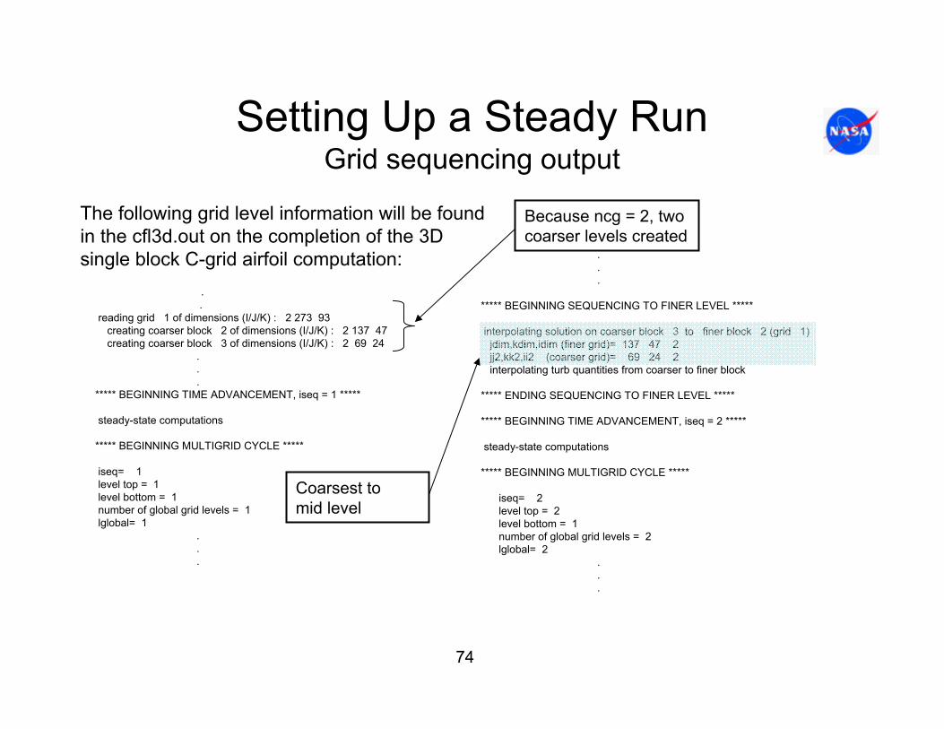
Setting Up a Steady RunGrid sequencing output
The following grid level information will be found in the cfl3d.out on the completion of the 3D single block C-grid airfoil computation:
..
reading grid 1 of dimensions (I/J/K) : 2 273 93creating coarser block 2 of dimensions (I/J/K) : 2 137 47creating coarser block 3 of dimensions (I/J/K) : 2 69 24
.
.
.***** BEGINNING TIME ADVANCEMENT, iseq = 1 *****
steady-state computations
***** BEGINNING MULTIGRID CYCLE *****
iseq= 1level top = 1level bottom = 1number of global grid levels = 1lglobal= 1
.
.
.
.
.
.
***** BEGINNING SEQUENCING TO FINER LEVEL *****
interpolating solution on coarser block 3 to finer block 2 (grid 1)jdim,kdim,idim (finer grid)= 137 47 2jj2,kk2,ii2 (coarser grid)= 69 24 2interpolating turb quantities from coarser to finer block
***** ENDING SEQUENCING TO FINER LEVEL *****
***** BEGINNING TIME ADVANCEMENT, iseq = 2 *****
steady-state computations
***** BEGINNING MULTIGRID CYCLE *****
iseq= 2level top = 2level bottom = 1number of global grid levels = 2lglobal= 2
.
.
.
Coarsest tomid level
Because ncg = 2, two coarser levels created

75
Setting Up a Steady RunGrid sequencing output
.
.
.
***** BEGINNING SEQUENCING TO FINER LEVEL *****
interpolating solution on coarser block 2 to finer block 1 (grid 1)jdim,kdim,idim (finer grid)= 273 93 2jj2,kk2,ii2 (coarser grid)= 137 47 2interpolating turb quantities from coarser to finer block
***** ENDING SEQUENCING TO FINER LEVEL *****
***** BEGINNING TIME ADVANCEMENT, iseq = 3 *****
steady-state computations
***** BEGINNING MULTIGRID CYCLE *****
iseq= 3level top = 3level bottom = 1number of global grid levels = 3lglobal= 3
Mid to finest level

76
Setting Up a Steady RunGrid sequencing
ncg iem iadvance iforce ivisc(i) ivisc(j) ivisc(k)2 0 0 1 0 0 5
.
.idim jdim kdim
2 273 93..
.mseq mgflag iconsf mtt ngam
3 1 0 0 2issc epsssc(1) epsssc(2) epsssc(3) issr epsssr(1) epsssr(2) epsssr(3)
0 0.3 0.3 0.3 0 0.3 0.3 0.3ncyc mglevg nemgl nitfo
2000 1 0 01000 2 0 0
500 3 0 0mit1 mit2 mit3 mit4 mit5 ...
1 1 1 1 1 1
Note:– The number of grid levels that will have been created are the coarser levels (ncg) plus the
finest level. Therefore, mseq must be equal to or less than ncg + 1. Setting mseq higher than this will result in a termination and an error message in precfl3d.out.
– The permissible value of ncg will depend on the dimensions of the grid. It is usually good to have three to four possible levels of multi-grid. For example, since four levels of multi-gridare possible with this grid, we could have set ncg = 3.
These dimensions support up tofour multigrid levels. See version 5.0manual for a table of multigridabledimensions. Note that idim is notmultigridded for a 2D grid.
77
Setting Up a Steady RunGrid sequencing
Note:– Many more cycles will be done at the coarser levels. The
computing required for a 3D grid will be a factor of 8 cheaper at each coarser level. For the present problem, the coarsest levelwould be 64 times cheaper than the finest level if a 3D grid hadbeen used. Since it is a 2D grid it will be 16 times cheaper.
– It is usually good to completely converge the coarser levels before proceeding to the finer level. However, some problems will not compute well at a coarse level, but will compute at a finer level.
– Mglevg is always starting from the finest level … as the following example will show…
78
Setting Up a Steady RunGrid sequencing
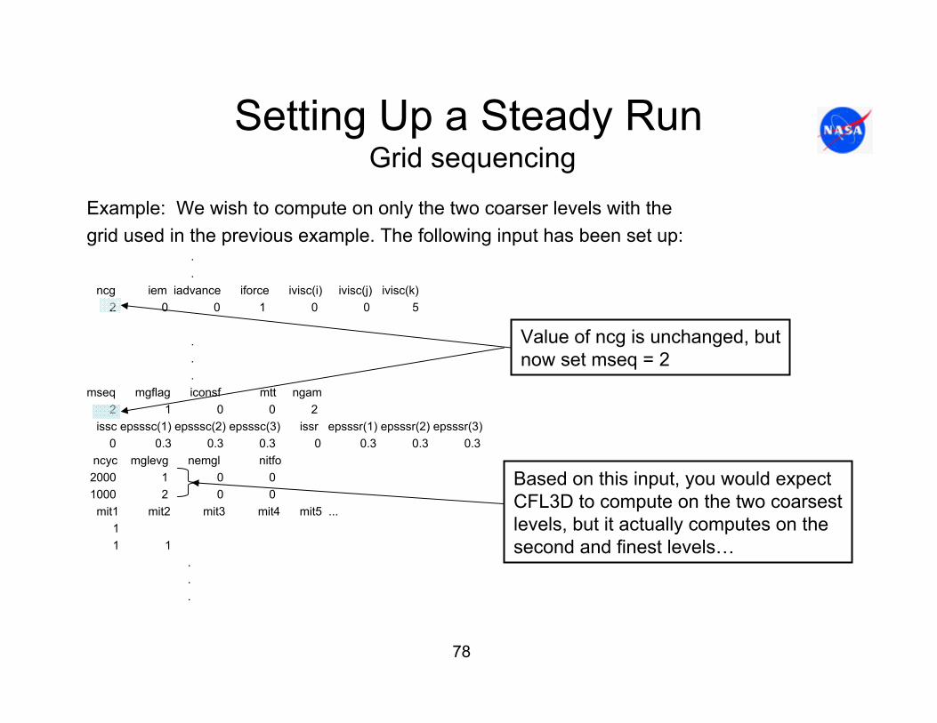
Example: We wish to compute on only the two coarser levels with the grid used in the previous example. The following input has been set up:
.
.ncg iem iadvance iforce ivisc(i) ivisc(j) ivisc(k)
2 0 0 1 0 0 5
.
.
.mseq mgflag iconsf mtt ngam
2 1 0 0 2issc epsssc(1) epsssc(2) epsssc(3) issr epsssr(1) epsssr(2) epsssr(3)
0 0.3 0.3 0.3 0 0.3 0.3 0.3ncyc mglevg nemgl nitfo2000 1 0 01000 2 0 0mit1 mit2 mit3 mit4 mit5 ...
1 1 1
.
.
.
Value of ncg is unchanged, butnow set mseq = 2
Based on this input, you would expect CFL3D to compute on the two coarsestlevels, but it actually computes on the second and finest levels…

79
Setting Up a Steady RunGrid sequencing
…Here is what is actually output in cfl3d.out:
***** BEGINNING TIME ADVANCEMENT, iseq = 1 *****
steady-state computations
***** BEGINNING MULTIGRID CYCLE *****
iseq= 1level top = 2level bottom = 2number of global grid levels = 1lglobal= 2
.
.
.
***** BEGINNING SEQUENCING TO FINER LEVEL *****
interpolating solution on coarser block 2 to finer block 1 (grid 1)jdim,kdim,idim (finer grid)= 273 93 2jj2,kk2,ii2 (coarser grid)= 137 47 2interpolating turb quantities from coarser to finer block
***** ENDING SEQUENCING TO FINER LEVEL *****
***** BEGINNING TIME ADVANCEMENT, iseq = 2 *****
steady-state computations
***** BEGINNING MULTIGRID CYCLE *****
iseq= 2level top = 3level bottom = 2number of global grid levels = 2lglobal= 3
Computations performed on the middle and finest grids

80
Setting Up a Steady RunGrid sequencing at coarsest levels only
Here is how to compute only on the two coarsest levels:..
ncg iem iadvance iforce ivisc(i) ivisc(j) ivisc(k)2 0 0 1 0 0 5
.
.
.mseq mgflag iconsf mtt ngam
3 1 0 0 2issc epsssc(1) epsssc(2) epsssc(3) issr epsssr(1) epsssr(2) epsssr(3)
0 0.3 0.3 0.3 0 0.3 0.3 0.3ncyc mglevg nemgl nitfo2000 1 0 01000 2 0 0
0 3 0 0mit1 mit2 mit3 mit4 mit5 ...
1 1 1 1 1 1
.
.
.
The finest level is included but withzero cycles
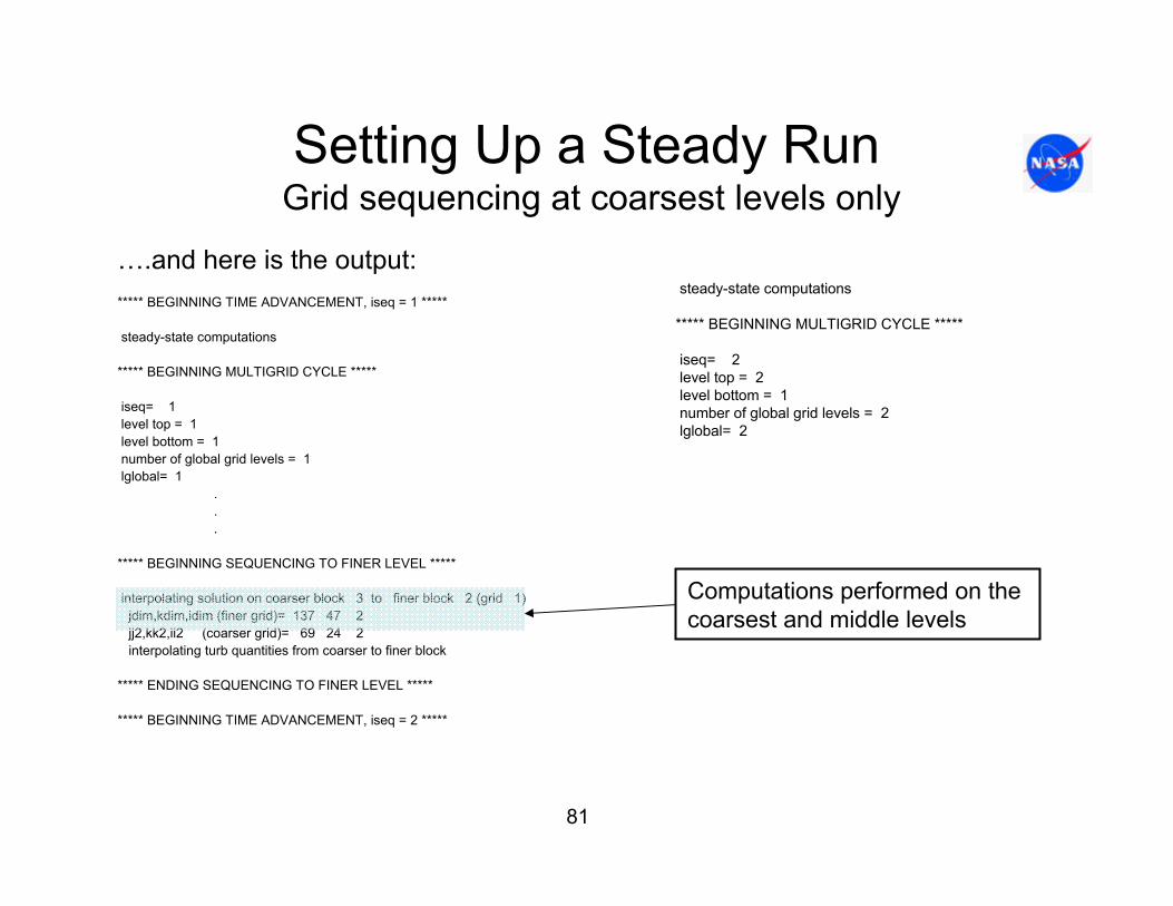
81
Setting Up a Steady RunGrid sequencing at coarsest levels only
….and here is the output:***** BEGINNING TIME ADVANCEMENT, iseq = 1 *****
steady-state computations
***** BEGINNING MULTIGRID CYCLE *****
iseq= 1level top = 1level bottom = 1number of global grid levels = 1lglobal= 1
.
.
.
***** BEGINNING SEQUENCING TO FINER LEVEL *****
interpolating solution on coarser block 3 to finer block 2 (grid 1)jdim,kdim,idim (finer grid)= 137 47 2jj2,kk2,ii2 (coarser grid)= 69 24 2interpolating turb quantities from coarser to finer block
***** ENDING SEQUENCING TO FINER LEVEL *****
***** BEGINNING TIME ADVANCEMENT, iseq = 2 *****
steady-state computations
***** BEGINNING MULTIGRID CYCLE *****
iseq= 2level top = 2level bottom = 1number of global grid levels = 2lglobal= 2
Computations performed on the coarsest and middle levels

82
Setting Up a Steady RunGrid sequencing at coarsest levels only
Why is it sometimes valuable to compute on the coarser levels only?
– Cost effectiveness of coarser levels– Sometimes it is not possible to converge the finest level– Many times you will want to compute unsteady solutions on
coarser levels only, especially when debugging. Computingunsteady solutions on coarser levels only requires the steady starting point be on a coarser level.

83
Setting Up a Steady RunRamping up dt
Sometimes it is useful for stiff problems to ramp up the time step size. Ramping up the time step size is accomplished with the following input:
dt irest iflagts fmax iunst cfl_tau-2.0 0 1000 5.0 0 5.0
dtending = fmax * dtinitial
dtinitial
In this example, the final CFL value of 10 is obtained after 1000 cycles. Notethat this counter is reset with each restart. Therefore, dtinitial will have to be reset to the dtending of the previous run.
No. of cycles over which time step ramping occurs
84
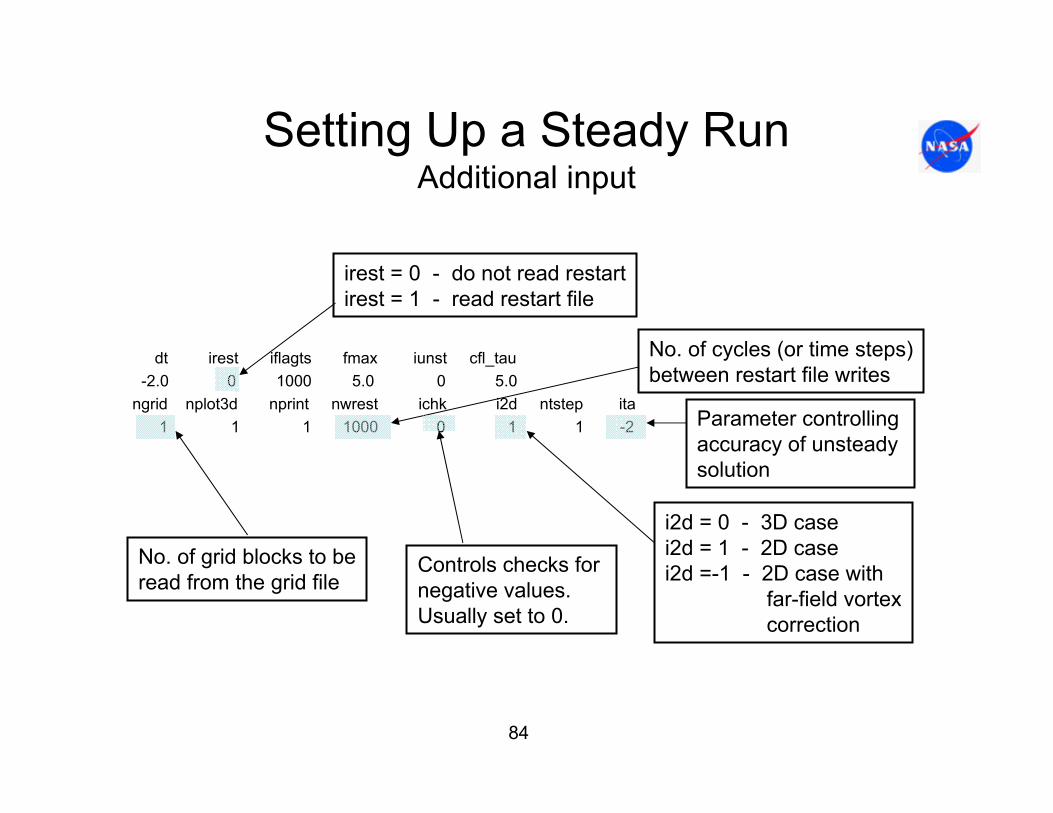
Setting Up a Steady RunAdditional input
dt irest iflagts fmax iunst cfl_tau-2.0 0 1000 5.0 0 5.0
ngrid nplot3d nprint nwrest ichk i2d ntstep ita1 1 1 1000 0 1 1 -2
irest = 0 - do not read restartirest = 1 - read restart file
No. of cycles (or time steps)between restart file writes
No. of grid blocks to beread from the grid file
Controls checks for negative values.Usually set to 0.
i2d = 0 - 3D casei2d = 1 - 2D casei2d =-1 - 2D case with
far-field vortexcorrection
Parameter controllingaccuracy of unsteady solution

85
Setting Up a Steady RunAdditional input
ncg iem iadvance iforce ivisc(i) ivisc(j) ivisc(k)2 0 0 1 0 0 5
idim jdim kdim2 273 93
This card repeated ngrid times
This card repeated ngrid times
Parameters controllinglevel of turbulence modelingin the i, j, k directions
Flag for residual/updateusually set to 0
Flag controlling force computations on blockFaces. Format is IJK, e.g. 100 calculates forceOn solid i=1 surfaces, 10 calculates force on solidj=1 surfaces, etc…. See version 5 manual for more
Embedded meshflag, usually 0

86
Setting Up a Steady RunTurbulence model input
There are more than 13 turbulence models available, but the following are the most common turbulence models and the corresponding parameter input values:
0 - inviscid1 - laminar3 - turbulent, Baldwin-Lomax with Degani-Schiff
option (not recommended)5 - turbulent, Spalart-Allmaras model6 - turbulent, Wilcox k-ω7 - turbulent, k-ω SST (Menter’s version)
13 - nonlinear EASM k-ε model14 - nonlinear EASM k-ω model
See the CFL3D Version 5.0 manual (Appendix H) and the CFL3D Version 6 web page (under `New Features’) for descriptions of these and other models. See also under the ‘Keywords’ discussion in these notes for parameters that turn turbulence model features on.

87
Setting Up a Steady RunTurbulence model
Several key notes on turbulence models:
1. If ivisc(m) < 0, a wall function is employed2. Thin-layer viscous terms (laminar or turbulent) can be included in the i,j or k
directions separately or combined. Cross-derivatives are not included. For the Baldwin-Lomax model, terms are allowed simultaneously in two directions only,either j-k or i-k.
3. Using the Baldwin-Lomax model with multi-zonal grids, wall distances are calculated only within a given zone.
4. It is preferable to let k be the primary viscous direction and i be secondary viscous direction.
5. The minimum distance function smin is computed from viscous walls only, not inviscid walls.

88
Setting Up a Steady RunTurbulence model
6. Note that the field equation turbulence models may or may not transition to turbulent flow. Whether they transition will largely be determined by the free stream value of turbulence. Free stream turbulence level can be set in the key word input.
7. There are several places in which the turbulence level can be checked– There is an option allows the output of turbulence quantities in the
plot3d file.– The file ‘cfl3d.prout’ contains the value of the turbulent viscosity. This is
shown in the next slide.
See the CFL3D User’s Manual, Version 5.0, Section 3.7 for more complete discussion

89
Setting Up a Steady RunTurbulence model output
The top of the ‘cfl3d.prout’ file is shown here:
NASA Langley BACT Model: NACA 0012 af, AR=1.5 wing,.75TE FlapMach alpha beta ReUe Tinf,dR time
0.82000 0.00000 0.00000 0.236E+07 486.00000 0.03839
BLOCK 1 (GRID 1) IDIM,JDIM,KDIM= 73 345 73NOTE: endpts may not be reliable
I J K X Y Z U/Uinf V/Vinf W/Winf P/Pinf T/Tinf MACH cp tur. vis.1 1 1 0.70000E+01 0.00000E+00 0.18698E-09 0.10000E+01 -0.38013E-18 0.72322E-13 0.10000E+01 0.10000E+01 0.82000E+00 0.50654E-07 0.90000E-021 2 1 0.68895E+01 0.00000E+00 0.18866E-09 0.10000E+01 -0.16458E-16 -0.14259E-15 0.10000E+01 0.10000E+01 0.82000E+00 0.50654E-07 0.90000E-02
.
.
Data lines will be printed out for all flow field points specified by the user in the ‘print out’ portion of the input file.
Turbulent viscosity

90
Setting Up a Steady RunMiscellaneous input
ilamlo ilamhi jlamlo jlamhi klamlo klamhi0 0 0 0 0 0
inewg igridc is js ks ie je ke0 0 0 0 0 0 0 0
Lower and upper i,j,k indices of laminarregion
This card repeated ngrid times
This card repeated ngrid times
Embedded mesh specifications. Zero ifno embedded mesh. See version 5.0 manual for more information

91
Setting Up a Steady RunMiscellaneous input
idiag(i) idiag(j) idiag(k) iflim(i) iflim(j) iflim(k)1 1 1 4 4 4
ifds(i) ifds(j) ifds(k) rkap0(i) rkap0(j) rkap0(k)1 1 1 0.3333 0.3333 0.3333
This card repeated ngrid times
This card repeated ngrid times
Spatial differencing in the i,j,k directions.ifds = 1 – flux-difference
splitting (Roe’s)(recommended)
Spatial differencing parameter for Euler fluxes in the i,j,k directions. rkap0 = 1/3 - upwind-biased third order (recommended)
Flux limiter flag in the i,j,k directions.iflim = 3 was recommended in Version 5.0iflim = 4 is recommended in Version 6.0

92
Setting Up an Unsteady RunInput for time advancement
input/output files:grid.binplot3dg.binplot3dq.bincfl3d.outcfl3d.rescfl3d.turrescfl3d.blomaxcfl3d.out15cfl3d.proutcfl3d.out20ovrlp.binpatch.binrestart.bin
NLR7301 airfoil, cfl3d type gridXmach alpha beta ReUe Tinf,dR ialph ihstry
0.753 1.10 0.0 5.7567 460.0 0 0sref cref bref xmc ymc zmc1.0 1.0 1.0 0.075 0.0 0.0dt irest iflagts fmax iunst cfl_tau
.05 1 0 1.0 0 5.0
ngrid nplot3d nprint nwrest ichk i2d ntstep ita1 1 1 1000 0 1 1 -2
ncg iem iadvance iforce ivisc(i) ivisc(j) ivisc(k)2 0 0 1 0 0 5
idim jdim kdim2 273 93
ilamlo ilamhi jlamlo jlamhi klamlo klamhi0 0 0 0 0 0
inewg igridc is js ks ie je ke0 0 0 0 0 0 0 0
idiag(i) idiag(j) idiag(k) iflim(i) iflim(j) iflim(k)1 1 1 4 4 4
ifds(i) ifds(j) ifds(k) rkap0(i) rkap0(j) rkap0(k)1 1 1 0.3333 0.3333 0.3333
.
.
.
mseq mgflag iconsf mtt ngam1 1 0 0 2
issc epsssc(1) epsssc(2) epsssc(3) issr epsssr(1) epsssr(2) epsssr(3)0 0.3 0.3 0.3 0 0.3 0.3 0.3
ncyc mglevg nemgl nitfo4 3 0 0
mit1 mit2 mit3 mit4 mit5 ... 1 1 1
We will again focus on these three lines

93
Setting Up an Unsteady RunInput for time advancement
Time step parameters:
dt irest iflagts fmax iunst cfl_tau.05 1 0 1.0 0 5.0
Number of time step advances, and time accuracy:
ngrid nplot3d nprint nwrest ichk i2d ntstep ita1 1 1 1000 0 1 100 -2
Iterative control:
ncyc mglevg nemgl nitfo4 3 0 0
Non-dimensional time step size
Number of time steps
Number of sub-iterations
Parameter controlling timeaccuracy and dual time stepping

94
Setting Up an Unsteady RunInput for time advancement
Order of time-accuracy, dual time scheme flag (ita)
ita = +1 First order accurate in time; physical time term only(t-TS) method
ita = +2 Second order accurate in time; physical time term only (t-TS) method
ita = -1 First order accurate in time; physical time and pseudo time term (τ-TS) method
ita = -2 Second order accurate in time; physical time and pseudo time term (τ-TS) method

95
Setting Up an Unsteady RunInput for time advancement
Note:
• The approximate factorization scheme used to advance the solution in time introduces first order errors in time. Furthermore, if the diagonal version is utilized (idiag = 1), additional errors of order ∆τ are introduced. Sub-iterations can be used to drive these factorization errors to zero. Therefore, if a formally second-order (in time) solution is desired, sub-iterations must be used.
• The inclusion of a pseudo time term increases (often dramatically) the maximum allowable time step one can take for a particular problem. However, sub-iterations (ncyc > 1) are therefore mandatory and multi-grid is highly recommended.
• Larger time steps imply greater error, therefore second order is recommended.• You will almost never want to use the t-TS method of time stepping.
96
Setting Up an Unsteady RunEquations for τ-TS time advancement
)())(1(
11
11m
nmnm
m
QRtJ
QQtJ
QJQ
QCBAItJJ
+∆
−+−∆
∆+∆
∆′
=∆⎥⎦
⎤⎢⎣
⎡ +++⎟⎠⎞
⎜⎝⎛
∆++
∆′+
−− φφτ
φ
δδδφτφ
ζηξ
Sub-iteration index
Current time step index
Non-dimensionaltime step increment
Pseudo time step increment

97
Setting Up an Unsteady RunEquations for t-TS time advancement
)())(1(
1
1m
nmn
m
QRtJ
QQtJ
Q
QCBAItJ
+∆
−+−∆
∆
=∆⎥⎦
⎤⎢⎣
⎡ +++⎟⎠⎞
⎜⎝⎛
∆+
− φφ
δδδφζηξ
Non-dimensional time step increment
The pseudo time terms are omitted for t-TS timeadvancement:
98
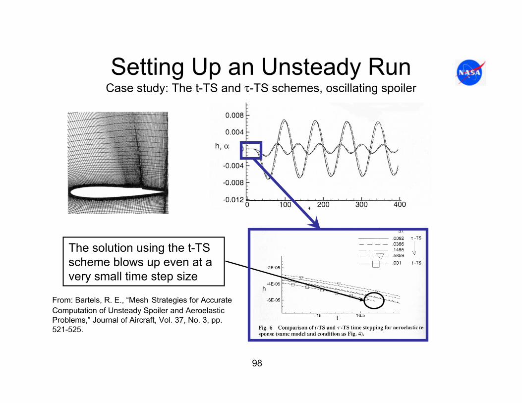
Setting Up an Unsteady RunCase study: The t-TS and τ-TS schemes, oscillating spoiler
The solution using the t-TS scheme blows up even at a very small time step size
From: Bartels, R. E., “Mesh Strategies for Accurate Computation of Unsteady Spoiler and AeroelasticProblems,” Journal of Aircraft, Vol. 37, No. 3, pp. 521-525.

99
Setting Up an Unsteady RunSpeeding up execution time
idiag(i) idiag(j) idiag(k) iflim(i) iflim(j) iflim(k)1 1 1 4 4 4
ifds(i) ifds(j) ifds(k) rkap0(i) rkap0(j) rkap0(k)1 1 1 0.3333 0.3333 0.3333
Parameters controlling the formof the Jacobian matrices used on the left hand side of the equations
Setting idiag(i), idiag(j), idiag(k) to 1 results in a very efficient trigiagonalinversion of the left hand side of the equations in the i, j and k directions.However, be aware of the implications of setting this …..
100
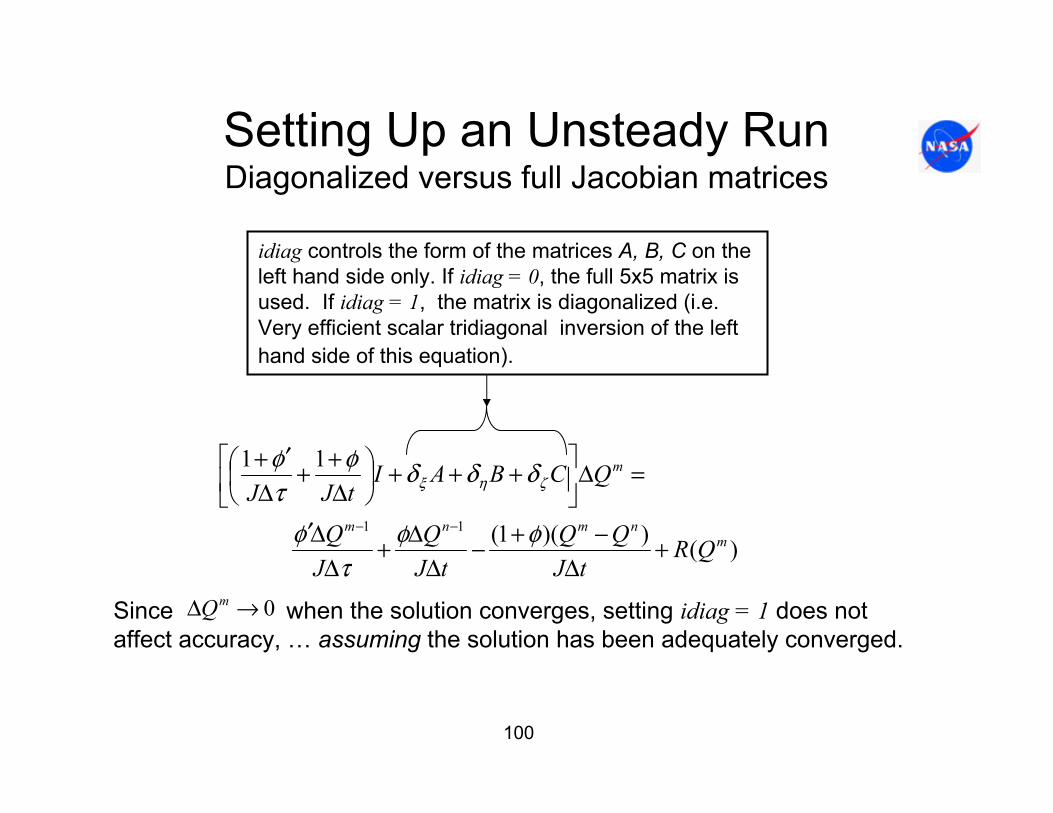
Setting Up an Unsteady RunDiagonalized versus full Jacobian matrices
)())(1(
11
11m
nmnm
m
QRtJ
QQtJ
QJQ
QCBAItJJ
+∆
−+−∆
∆+∆
∆′
=∆⎥⎦
⎤⎢⎣
⎡ +++⎟⎠⎞
⎜⎝⎛
∆++
∆′+
−− φφτ
φ
δδδφτφ
ζηξ
idiag controls the form of the matrices A, B, C on the left hand side only. If idiag = 0, the full 5x5 matrix is used. If idiag = 1, the matrix is diagonalized (i.e. Very efficient scalar tridiagonal inversion of the left hand side of this equation).
Since when the solution converges, setting idiag = 1 does not affect accuracy, … assuming the solution has been adequately converged.
0→∆ mQ
101
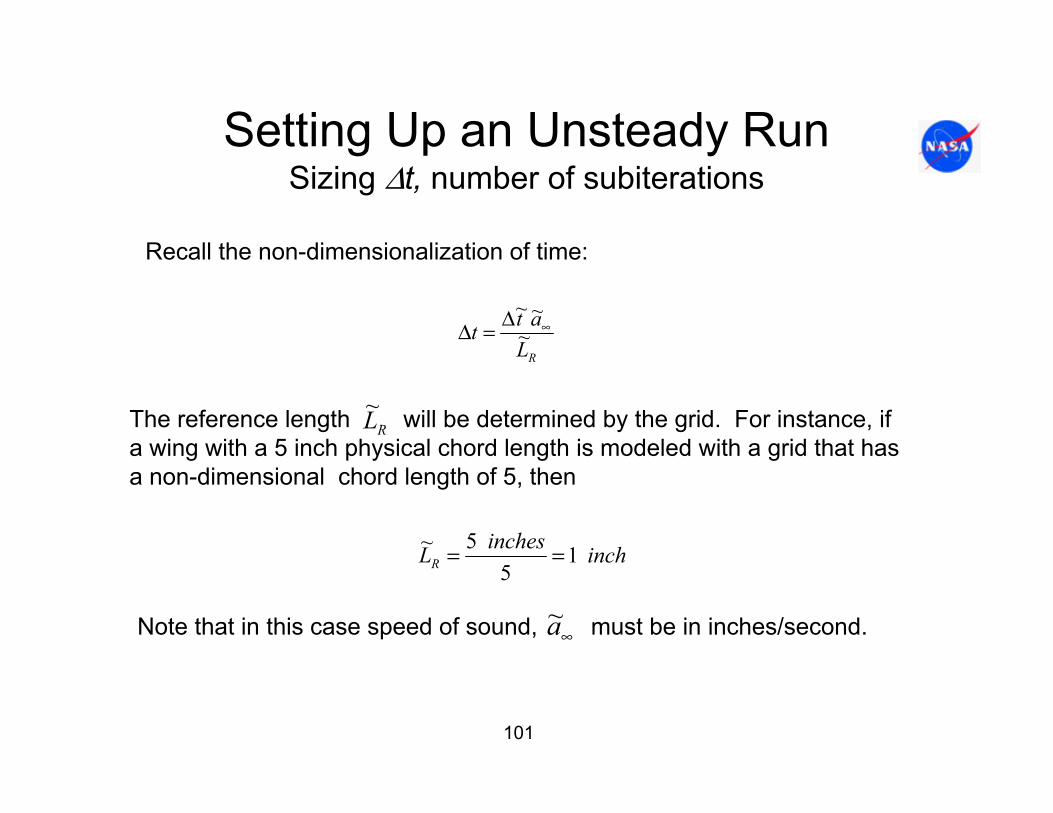
The reference length will be determined by the grid. For instance, ifa wing with a 5 inch physical chord length is modeled with a grid that has a non-dimensional chord length of 5, then
Setting Up an Unsteady RunSizing ∆t, number of subiterations
RL~
inchinchesLR 15
5~ ==
Note that in this case speed of sound, must be in inches/second.∞a~
Recall the non-dimensionalization of time:
RLatt ~~~
∞∆=∆

102
Setting Up an Unsteady RunSizing ∆t, number of subiterations
• One criteria for time step sizing is the time scale required to resolve a phenomenon at some frequency. Another is the number of time stepsfor a flow field particle to pass over a chord length. Consider 100 time steps per cycle or 100 time steps to pass over a chord length as the absolute minimum, which ever is smaller.
• The time step size and the number of sub-iterations may have to be set lower/higher respectively by either accuracy or robustness requirements. Short test runs should be performed to ensureadequate convergence.

103
Setting Up an Unsteady RunSizing ∆t, number of subiterations
• Indicators that the time step size is too large:• The solution converges very slowly or does not converge at all.• The solution simply blows up. • There are large numbers of negative turbulence parameter values
in the file ‘cfl3d.subit_turres’ the number of which is not converging towardzero at the end of each time step.
• Indicator that the number of sub-iterations is too small:• The force coefficients have not leveled out to an acceptable
convergence level.• The residuals have dropped only by an insufficient magnitude. This
can also be a sign that the time step is too large.• The solution has been converging, but eventually blows up or
starts to gradually diverge.• Note that these symptoms can also be due to problems with the grid,
boundary conditions or turbulence model, so first ensure these issues are settled.
104
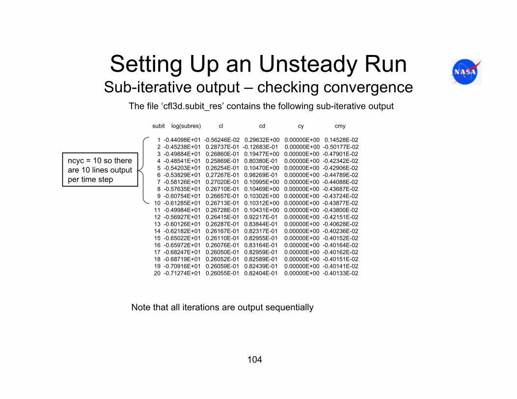
Setting Up an Unsteady RunSub-iterative output – checking convergence
The file ‘cfl3d.subit_res’ contains the following sub-iterative output
subit log(subres) cl cd cy cmy
1 -0.44098E+01 -0.56246E-02 0.29632E+00 0.00000E+00 0.14528E-022 -0.45238E+01 0.28737E-01 -0.12683E-01 0.00000E+00 -0.50177E-023 -0.49884E+01 0.26860E-01 0.19477E+00 0.00000E+00 -0.47901E-024 -0.48541E+01 0.25869E-01 0.80380E-01 0.00000E+00 -0.42342E-025 -0.54203E+01 0.26254E-01 0.10470E+00 0.00000E+00 -0.42906E-026 -0.53829E+01 0.27267E-01 0.98269E-01 0.00000E+00 -0.44789E-027 -0.58126E+01 0.27020E-01 0.10995E+00 0.00000E+00 -0.44088E-028 -0.57635E+01 0.26710E-01 0.10469E+00 0.00000E+00 -0.43687E-029 -0.60754E+01 0.26657E-01 0.10302E+00 0.00000E+00 -0.43724E-02
10 -0.61285E+01 0.26713E-01 0.10312E+00 0.00000E+00 -0.43877E-0211 -0.49984E+01 0.26728E-01 0.10431E+00 0.00000E+00 -0.43800E-0212 -0.56927E+01 0.26415E-01 0.92217E-01 0.00000E+00 -0.42151E-0213 -0.60126E+01 0.26287E-01 0.83844E-01 0.00000E+00 -0.40628E-0214 -0.62182E+01 0.26167E-01 0.82317E-01 0.00000E+00 -0.40236E-0215 -0.65022E+01 0.26110E-01 0.82955E-01 0.00000E+00 -0.40152E-0216 -0.65972E+01 0.26076E-01 0.83164E-01 0.00000E+00 -0.40164E-0217 -0.68247E+01 0.26050E-01 0.82959E-01 0.00000E+00 -0.40162E-0218 -0.68719E+01 0.26052E-01 0.82589E-01 0.00000E+00 -0.40151E-0219 -0.70916E+01 0.26059E-01 0.82439E-01 0.00000E+00 -0.40141E-0220 -0.71274E+01 0.26055E-01 0.82404E-01 0.00000E+00 -0.40133E-02
Note that all iterations are output sequentially
ncyc = 10 so there are 10 lines outputper time step
105
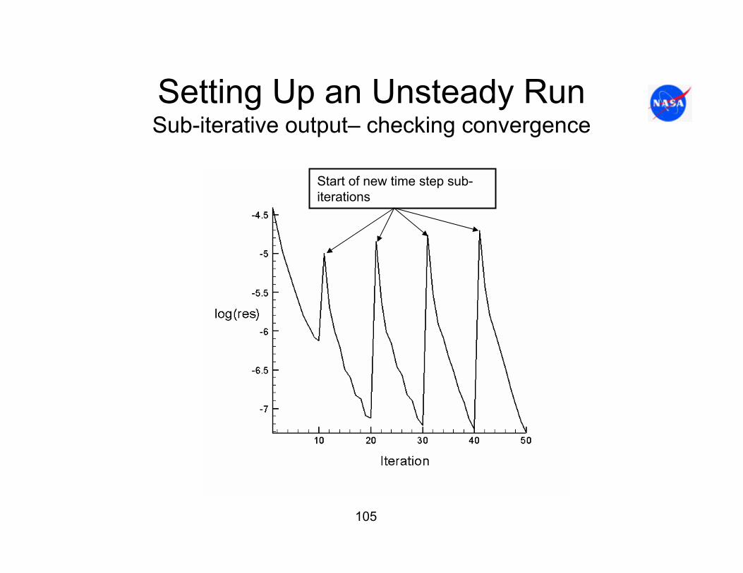
Setting Up an Unsteady RunSub-iterative output– checking convergence
Start of new time step sub-iterations
106
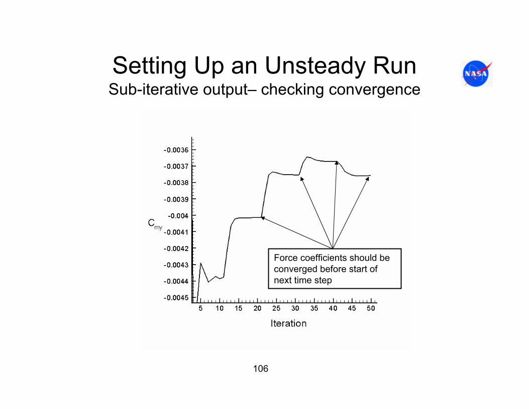
Setting Up an Unsteady RunSub-iterative output– checking convergence
Force coefficients should beconverged before start of next time step

107
Setting Up an Unsteady RunSub-iterative turbulence output
subit log(turres1) log(turres2) nneg1 nneg21 -0.73658E+01 -0.92553E+01 0 7102 -0.74563E+01 -0.91092E+01 0 823 -0.76424E+01 -0.90767E+01 0 24 -0.80379E+01 -0.90899E+01 0 05 -0.82466E+01 -0.93470E+01 0 86 -0.84600E+01 -0.93751E+01 0 307 -0.86186E+01 -0.95757E+01 0 588 -0.88672E+01 -0.97150E+01 0 569 -0.89497E+01 -0.98376E+01 0 48
10 -0.91579E+01 -0.99516E+01 0 38....
51 -0.95921E+01 -0.88827E+01 2498 214952 -0.95925E+01 -0.90172E+01 2340 269353 -0.95509E+01 -0.91643E+01 2124 260354 -0.99381E+01 -0.90386E+01 1959 119355 -0.98511E+01 -0.91025E+01 2244 125256 -0.99244E+01 -0.92361E+01 3529 139357 -0.10161E+02 -0.91691E+01 2373 148658 -0.10217E+02 -0.91525E+01 1395 136059 -0.10304E+02 -0.92210E+01 1266 146060 -0.10377E+02 -0.93327E+01 1109 1218
Note that there are a few grid points that have negative valuesof k and ω initially…
…however, large numbers of negative values of turbulencemodel parameters indicate a potential problem
In this case ncyc = 10 so there are 10 turbulence model iterations per time step.
Even though the turbulence model appears to be converging well, a large number of negative values may mean that the time step size is too large for the turbulence model. Usually reducing time step size will fix this problem.
The file ‘cfl3d.subit_turres’ contains the following sub-iterative outputfor Menter’s shear stress transport (SST) k-w turbulence model:

108
Setting Up an Unsteady RunMultigrid strategies
• Multigrid is a must for unsteady computations. The following input section establishes four multigrid sub-iterations each on three levels, the third being the finest:
mseq mgflag iconsf mtt ngam1 1 0 0 2
issc epsssc(1) epsssc(2) epsssc(3) issr epsssr(1) epsssr(2) epsssr(3)0 0.3 0.3 0.3 0 0.3 0.3 0.3
ncyc mglevg nemgl nitfo4 3 0 0
mit1 mit2 mit3 mit4 mit5 ... 1 1 1
Correction and residualsmoothing, typicallynot used (issc=issr=0)
Mesh sequencing andmultigrid parameters
Multigrid cyclingparameters
Number of iterations for each level, mitL = 1 recommended

109
Setting Up an Unsteady RunMultigrid strategies
mseq mgflag iconsf mtt ngam1 1 0 0 2
issc epsssc(1) epsssc(2) epsssc(3) issr epsssr(1) epsssr(2) epsssr(3)0 0.3 0.3 0.3 0 0.3 0.3 0.3
ncyc mglevg nemgl nitfo4 3 0 0
mit1 mit2 mit3 mit4 mit5 ... 1 1 1
Note:• iconsf is a parameter for setting conservative flux treatment for embedded grids. For
most computations it is set to zero.• mtt is a flag for additional iterations on the up portion of the multigrid. Recommend
setting to zero.• ngam is the multigrid cycle flag. ngam = 1 sets V-cycle, ngam = 2 sets a W-cycle. The
W-cycle is not recommended for overlapped grids.• mglevg is the number of grids to use in multigrid cycling. E.g. mglevg = 1 sets the finest
grid level only, mglevg = 2 sets two grid levels, etc…• nemgl is set to zero when there are no embedded grids.• nitfo1 is the number of first order iterations. Zero is recommended.

110
Setting Up an Unsteady RunMultigrid strategies
What if you want to compute an unsteady solution using multigrid on coarser levels only? Assume that the steady starting solution has been performed on coarser levels only, as we previously discussed. The following input will allow you to perform the unsteady run:
mseq mgflag iconsf mtt ngam2 1 0 0 2
issc epsssc(1) epsssc(2) epsssc(3) issr epsssr(1) epsssr(2) epsssr(3)0 0.3 0.3 0.3 0 0.3 0.3 0.3
ncyc mglevg nemgl nitfo4 2 0 00 3 0 0
mit1 mit2 mit3 mit4 mit5 ... 1 11 1 1
Note that a line with 0 sub-iterationsis included for a 3 level multigrid

111
Setting Up an Unsteady RunMultigrid strategies
….and here is the output:..
reading grid 1 of dimensions (I/J/K) : 2 273 93creating coarser block 2 of dimensions (I/J/K) : 2 137 47creating coarser block 3 of dimensions (I/J/K) : 2 69 24
.
.
.reading restart file for block 2 (grid 1)reading vist3d data from restart file, block 2reading field eqn turb quantities from restart file, block 2
.
.
. ***** BEGINNING MULTIGRID CYCLE *****
iseq= 1level top = 2level bottom = 1number of global grid levels = 2lglobal= 2
The full grid is read, and twocoarser levels created
This level is the finest on which computations are performed
Restart data is read for coarser block 2 only
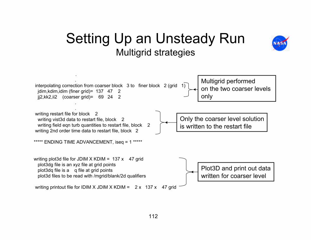
112
Setting Up an Unsteady RunMultigrid strategies
..
interpolating correction from coarser block 3 to finer block 2 (grid 1)jdim,kdim,idim (finer grid)= 137 47 2 jj2,kk2,ii2 (coarser grid)= 69 24 2
.
.writing restart file for block 2
writing vist3d data to restart file, block 2writing field eqn turb quantities to restart file, block 2
writing 2nd order time data to restart file, block 2
***** ENDING TIME ADVANCEMENT, iseq = 1 *****
writing plot3d file for JDIM X KDIM = 137 x 47 gridplot3dg file is an xyz file at grid pointsplot3dq file is a q file at grid pointsplot3d files to be read with /mgrid/blank/2d qualifiers
writing printout file for IDIM X JDIM X KDIM = 2 x 137 x 47 grid
Only the coarser level solutionis written to the restart file
Multigrid performed on the two coarser levels only
Plot3D and print out datawritten for coarser level

113
User Specified Grid MotionOverview
CFL3D has the capability to perform computations for prescribed surface motion in two ways
1. Prescribed, or user specified rigid grid motion. In this mode, the entire grid or set of grids translates or rotates in a manner prescribed by user input.
2. Prescribed surface motion with deforming mesh. In this mode, the surface(s) prescribed by the user translate or rotate and the meshdeforms accordingly.
These types of motion are only available when the code is running in unsteady mode.
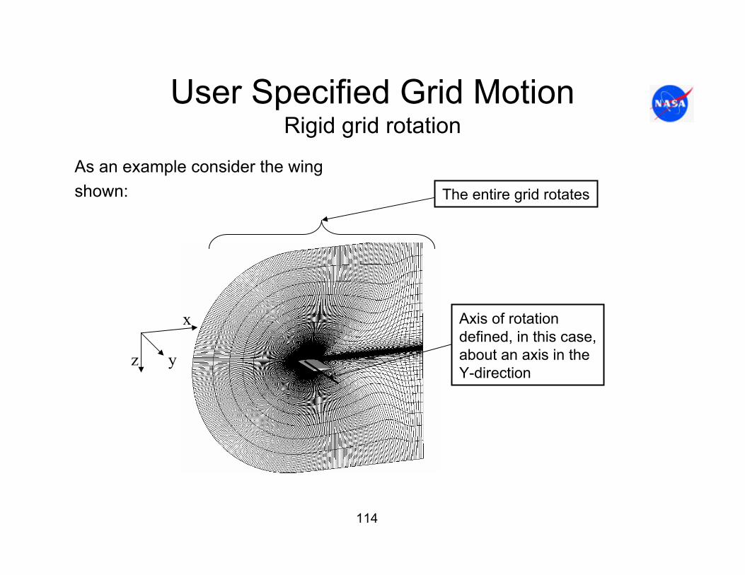
114
User Specified Grid MotionRigid grid rotation
As an example consider the wing shown:
x
z y
Axis of rotationdefined, in this case,about an axis in theY-direction
The entire grid rotates

115
User Specified Rigid Grid MotionRigid grid rotation
The following unsteady input file performs rotation about the axis shown:input/output files:
wbgrid.cflplot3dg.bin plot3dq.bin cfl3d.out cfl3d.rescfl3d.turres cfl3d.blomaxcfl3d.out15 cfl3d.prout cfl3d.out20 ovrlp.binpatch.binrestart.bin
NASA Langley BACT Model: NACA 0012 af, AR=1.5 wing,.75TE FlapMach alpha beta ReUe Tinf,dR ialph ihstry
0.82000 0.00000 0.00000 0.236E+07 486.00 1 0sref cref bref xmc ymc zmc
1.000 1.00000 1.00000 0.25000 0.00000 0.00000dt irest iflagts fmax iunst cfl_tau
0.04000 0 3000 1.00000 1 2.00000ngrid nplot3d nprint nwrest ichk i2d ntstep ita
1 1 1 1000 0 0 1 -2
Note that iunst = 1 for rigidtranslation or rotation
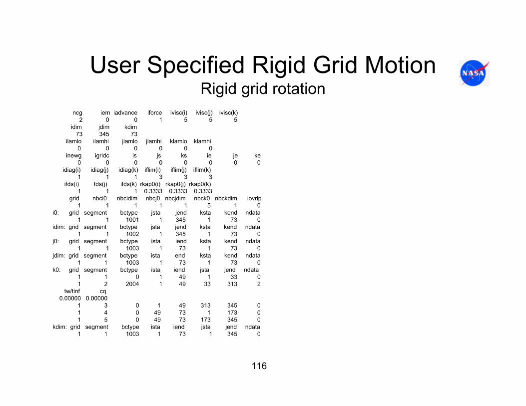
116
User Specified Rigid Grid MotionRigid grid rotation
ncg iem iadvance iforce ivisc(i) ivisc(j) ivisc(k)2 0 0 1 5 5 5
idim jdim kdim73 345 73
ilamlo ilamhi jlamlo jlamhi klamlo klamhi0 0 0 0 0 0
inewg igridc is js ks ie je ke0 0 0 0 0 0 0 0
idiag(i) idiag(j) idiag(k) iflim(i) iflim(j) iflim(k)1 1 1 3 3 3
ifds(i) fds(j) ifds(k) rkap0(i) rkap0(j) rkap0(k)1 1 1 0.3333 0.3333 0.3333
grid nbci0 nbcidim nbcj0 nbcjdim nbck0 nbckdim iovrlp1 1 1 1 1 5 1 0
i0: grid segment bctype jsta jend ksta kend ndata1 1 1001 1 345 1 73 0
idim: grid segment bctype jsta jend ksta kend ndata1 1 1002 1 345 1 73 0
j0: grid segment bctype ista iend ksta kend ndata1 1 1003 1 73 1 73 0
jdim: grid segment bctype ista end ksta kend ndata1 1 1003 1 73 1 73 0
k0: grid segment bctype ista iend jsta jend ndata1 1 0 1 49 1 33 01 2 2004 1 49 33 313 2
tw/tinf cq0.00000 0.00000
1 3 0 1 49 313 345 01 4 0 49 73 1 173 01 5 0 49 73 173 345 0
kdim: grid segment bctype ista iend jsta jend ndata 1 1 1003 1 73 1 345 0
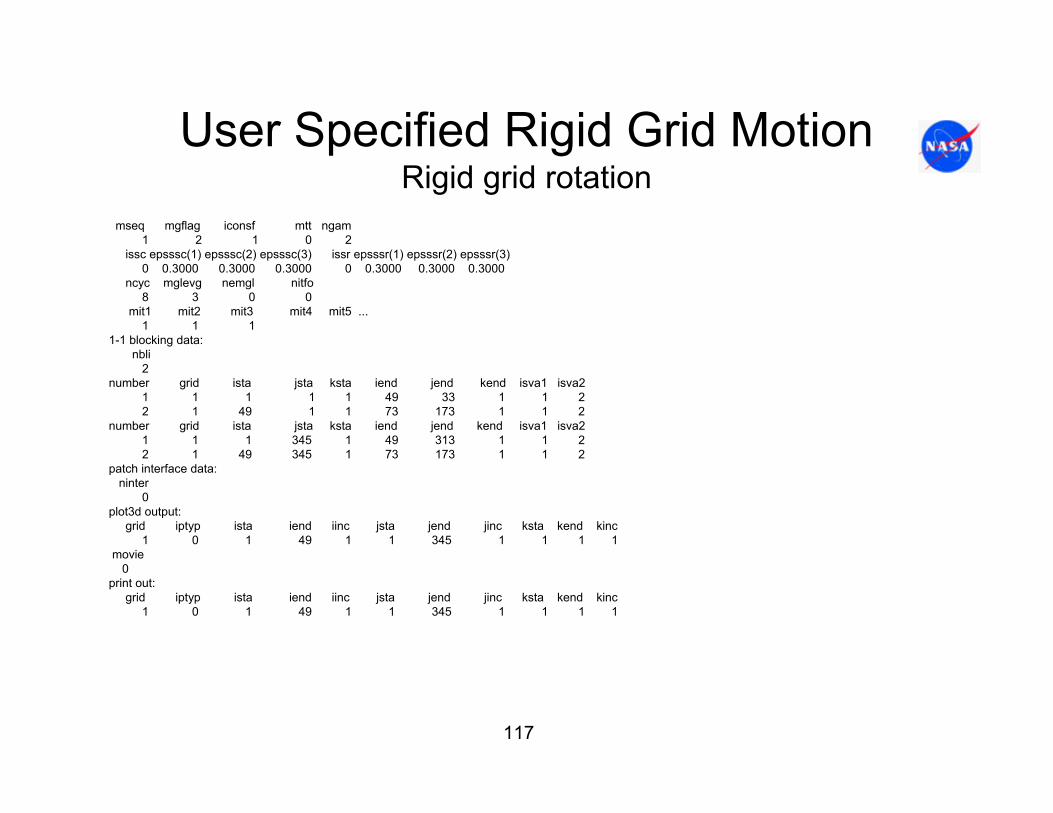
117
User Specified Rigid Grid MotionRigid grid rotation
mseq mgflag iconsf mtt ngam1 2 1 0 2
issc epsssc(1) epsssc(2) epsssc(3) issr epsssr(1) epsssr(2) epsssr(3)0 0.3000 0.3000 0.3000 0 0.3000 0.3000 0.3000
ncyc mglevg nemgl nitfo8 3 0 0
mit1 mit2 mit3 mit4 mit5 ...1 1 1
1-1 blocking data:nbli
2number grid ista jsta ksta iend jend kend isva1 isva2
1 1 1 1 1 49 33 1 1 22 1 49 1 1 73 173 1 1 2
number grid ista jsta ksta iend jend kend isva1 isva21 1 1 345 1 49 313 1 1 2 2 1 49 345 1 73 173 1 1 2
patch interface data:ninter
0plot3d output:
grid iptyp ista iend iinc jsta jend jinc ksta kend kinc1 0 1 49 1 1 345 1 1 1 1
movie0
print out:grid iptyp ista iend iinc jsta jend jinc ksta kend kinc
1 0 1 49 1 1 345 1 1 1 1

118
User Specified Rigid Grid MotionRigid grid rotation input
control surfaces:ncs
0grid ista iend jsta jend ksta kend iwall inorm
moving grid data - rigid translation (forced motion):ntrans
0 lref
grid itrans rfreq utrans vtrans wtransgrid dxmax dymax dzmax
moving grid data - rigid rotation (forced motion):nrotat
1lref1.0
grid irotat rfreq omegax omegay omegaz xorig yorig zorig1 2 0.05 0.00 5.00 0.00 0.25 0.00 0.00
grid dthxmx dthymx dthzmx1 10. 10. 10.
Patched data:ninter2
0
Rigid translation input. Note that ntrans = 0, so that only remaining header lines are included.
Rigid rotation input
The following lines mustbe included when iunst = 1

119
User Specified Rigid Grid MotionRigid grid rotation input
Focusing attention on the rigid rotation input:
moving grid data - rigid rotation (forced motion):nrotat
1lref1.0
grid irotat rfreq omegax omegay omegaz xorig yorig zorig1 2 0.05 0.00 5.00 0.00 0.25 0.00 0.00
grid dthxmx dthymx dthzmx1 10. 10. 10.
Number of grid blocks to be rotated
Line repeated nrotat times
Line repeated nrotat times
Reference length for reduced frequency

120
User Specified Rigid Grid MotionRigid grid rotation input
Focusing on the last two lines of input on the last slide:..
grid irotat rfreq omegax omegay omegaz xorig yorig zorig1 2 0.05 0.00 5.00 0.00 0.25 0.00 0.00
grid dthxmx dthymx dthzmx1 10. 10. 10.
.
.
grid - Grid block to be rotatedirotat - Type of rotation
= 0 - no rotation= 1 - rotation with constant angular speed= 2 - sinusoidal variation of angular displacement= 3 - smooth increase in displacement,
asymptotically reaching a maximum anglerfreq - reduced frequency when irotat = 2; growth rate to maximum angular displacement when
irotat = 3

121
User Specified Rigid Grid MotionRigid grid rotation input
.
.grid irotat rfreq omegax omegay omegaz xorig yorig zorig
1 2 0.05 0.00 5.00 0.00 0.25 0.00 0.00grid dthxmx dthymx dthzmx
1 10. 10. 10...
omegax, omegay, omegaz - x,y,z components of rotational velocity when irotat = 1; maximum angular displacements about x,y,z-axes when irotat > 1
xorig, yorig, zorig - x,y,z coordinate of origin of the rotational axis
dthymx, dthymx,dthzmx - maximum (absolute) rotational displacement about the x,y,z-axes to be allowed for this grid (set dthxmx,dthymx, dthzmx = 0 if no restriction is required)

122
User Specified Rigid Grid MotionRigid grid rotation input
Example of sinusoidal rotational motion irotat = 2. The following terms are defined:
The rotational displacement (radians) within the code is governed by
Based on these equations of sinusoidal motion,
where N is the desired number of time steps per cycle. Consult Chapter 4 of the Version 5.0 User’s Manual pp. 55-62 for details on all types of motion.
.deg,~,.deg,~,.deg,~,
max,max,max, zyx
refr
omegazomegayomegax
Llrefkrfreq
θθθ ===
==
)2sin(180
~
)2sin(180
~,)2sin(180
~
max,
max,max,
refrzz
refryy
refrxx
Ltk
Ltk
Ltk
ππθθ
ππθθππθθ
=
==
NkL
tr
ref=∆

123
User Specified Rigid Grid MotionRigid grid rotation
The following diagnostic information on the rotation of the surface(s) will be printed in ‘cfl3d.out’:
.
.
.rotating block 1 to new position creating coarser block 2 of dimensions (I/J/K) : 37 173 37restricting grid speeds from finer block 1 to coarser block 2
creating coarser block 3 of dimensions (I/J/K) : 19 87 19restricting grid speeds from finer block 2 to coarser block 3
.
.
.writing restart file for block 1
writing vist3d data to restart file, block 1writing field eqn turb quantities to restart file, block 1
writing 2nd order time data to restart file, block 1writing dynamic mesh data to restart file, block 1
.
.
.
Note that new dynamic mesh datahas been written to the restart file
Grid speed information computedfor moving grid

124
User Specified Rigid Grid MotionRigid grid translation input
.
.control surfaces:
ncs0
grid ista iend jsta jend ksta kend iwall inormmoving grid data - rigid translation (forced motion):
ntrans1
lref1.0
grid itrans rfreq utrans vtrans wtrans1 2 0.05 0.00 0.00 5.00
grid dxmax dymax dzmax1 10. 10. 10.
moving grid data - rigid rotation (forced motion):nrotat
0lref
grid irotat rfreq omegax omegay omegaz xorig yorig zoriggrid dthxmx dthymx dthzmxPatched data:ninter2
0
Rigid rotation input. Note that nrotat = 0, so that only remaining header lines are included.
Rigid translation input
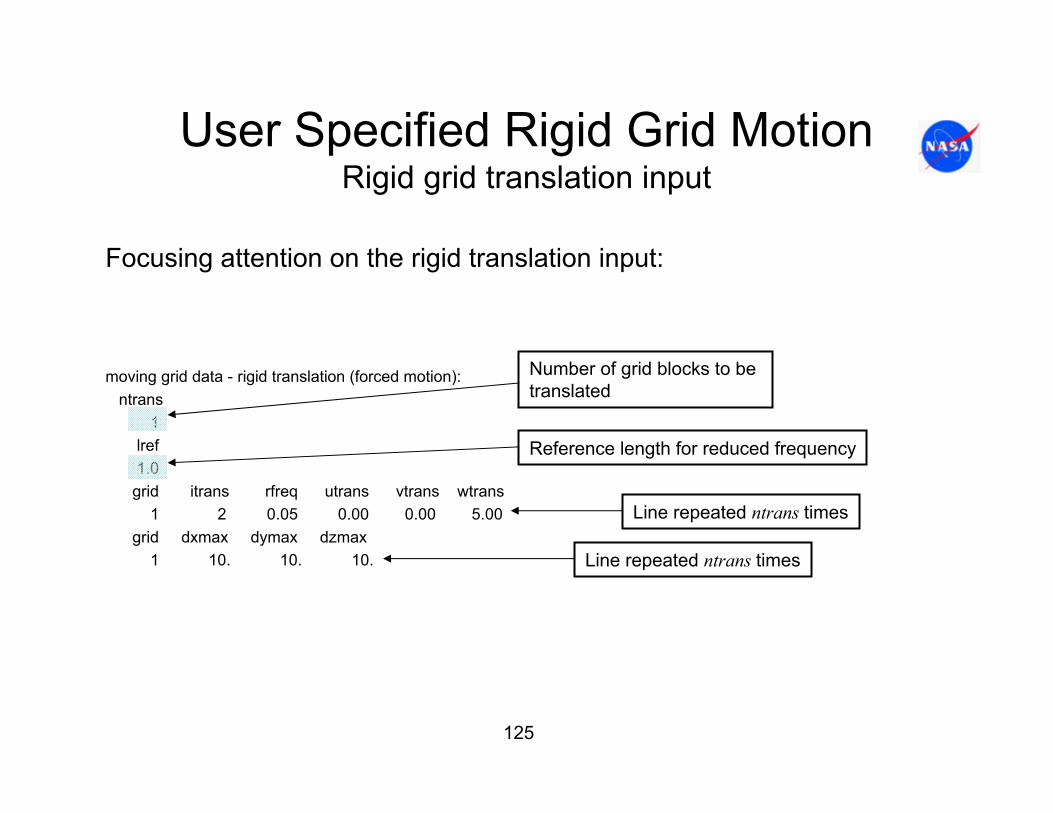
125
User Specified Rigid Grid MotionRigid grid translation input
Focusing attention on the rigid translation input:
moving grid data - rigid translation (forced motion):ntrans
1 lref1.0
grid itrans rfreq utrans vtrans wtrans1 2 0.05 0.00 0.00 5.00
grid dxmax dymax dzmax1 10. 10. 10.
Number of grid blocks to be translated
Line repeated ntrans times
Line repeated ntrans times
Reference length for reduced frequency
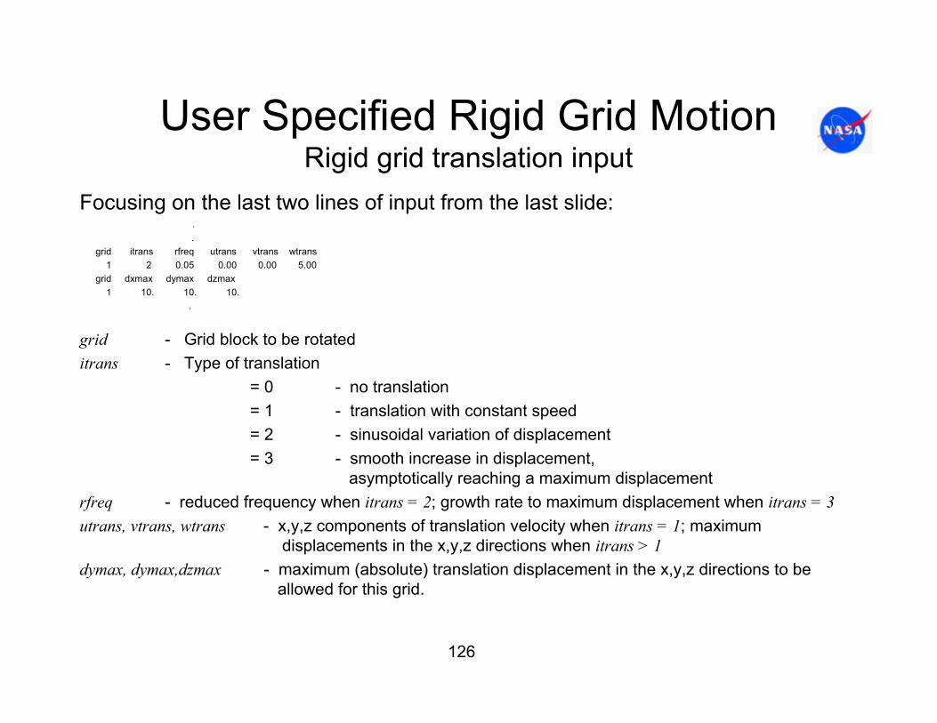
126
User Specified Rigid Grid MotionRigid grid translation input
Focusing on the last two lines of input from the last slide:..
grid itrans rfreq utrans vtrans wtrans1 2 0.05 0.00 0.00 5.00
grid dxmax dymax dzmax1 10. 10. 10.
.
grid - Grid block to be rotateditrans - Type of translation
= 0 - no translation= 1 - translation with constant speed= 2 - sinusoidal variation of displacement= 3 - smooth increase in displacement,
asymptotically reaching a maximum displacementrfreq - reduced frequency when itrans = 2; growth rate to maximum displacement when itrans = 3utrans, vtrans, wtrans - x,y,z components of translation velocity when itrans = 1; maximum
displacements in the x,y,z directions when itrans > 1dymax, dymax,dzmax - maximum (absolute) translation displacement in the x,y,z directions to be
allowed for this grid.
127
Surface Motion - Deforming MeshOverview
• CFL3D can perform several types of user specified surface motionby deforming the mesh, i.e. surface rotation and/or translation of all or partial segments of the solid surfaces as well as modal motion of surfaces.
• Aeroelastic, user defined deforming mesh surface and user defined rigid grid motion can be performed in any combination.
• There are two methods of deforming the mesh.– Exponential decay combined with Trans-Finite Interpolation (TFI) of
interior mesh points.– Finite macro-element deformation combined with TFI.
• Note that deforming surface motion can only be performed with the code running in unsteady mode.
128
Surface Motion - Deforming MeshOverview
• In the first mesh movement option (exponential decay method) deformation is performed in two steps.
– The first step is exponential decay of control points away from the moving surface. The rate of the exponential decay is controlled by user input.
– The second step is a TFI of mesh points interior to the control points. • Advantage of the exponential decay method is that it is computationally efficient• In the second mesh movement option (finite macro-element method) deformation is
also performed in two steps. – The first step is a finite element solution of macro-element points. The resulting solution
transmits surface motion to the element node points. The element stiffness varies with distance from the surface. User specified input controls the rate at which the element stiffness decays away from surfaces.
– The second step is a TFI of mesh points interior to the element node (or control) points. – See Bartels, R. E., “Finite Macro-Element Mesh Deformation in a Structured Multi-Block
Navier-Stokes Code,” NASA/TM-2005-213789, July 2005.• Advantage of the finite macro-element method is that it maintains mesh quality, but is
significantly more computationally time consuming.

129
Surface Motion - Deforming MeshDeforming mesh terminology
Control point, also called node point - member of a sub-grid set of mesh points
An exteriorface of theflow fieldblock
Deforminggrid surface, e.g.wing surface
Sub-grid surfacepoint
CFDmeshpoints

130
Surface Motion - Deforming MeshDeforming mesh using exponential decay method
)/(
],1min[
)(
2max2
11
αβ −∆∆=
=
−=−
−
++
rrAand
eDwhere
rrDrr
sc
Asc
ns
nssc
nc
nc
r
rrrr
Nearestsurface sub-grid point, s
Controlpoint, c
∆rsc
The movement of surface points is transmitted into the flow field sub-grid through an exponential decay function Dsc . The rate of decay is controlledby the parameters β2 and α2.

131
Surface Motion - Deforming MeshDeforming mesh with exponential decay method
Note several potential draw backs to this approach:
• Too rapid a rate of decay (β2 too large, α2 too small) results in the possibility of the surface points moving through nearby control points.
• Too low a rate of decay (β2 too small, α2 too large) results in the possibility of surface deformation being transmitted too far into the flow field with possible penetration of opposing surfaces.
• Typical values for decay parameters are:
β2 = 1 - 10 , α2 = 0.005 – 0.05

132
Surface Motion - Deforming MeshTrans-Finite Interpolation (TFI) of interior points
Mesh points interior to the sub-block face are inter-polated using deflection of four corner control points
The final step is a volume TFI ofinterior grid points based on locationsof mesh points on the sub-block faces
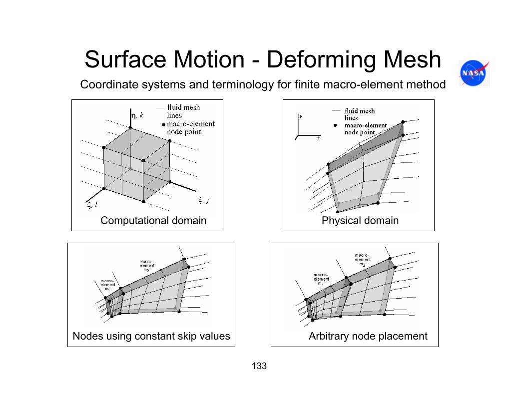
133
Surface Motion - Deforming MeshCoordinate systems and terminology for finite macro-element method
Computational domain Physical domain
Nodes using constant skip values Arbitrary node placement

134
Surface Motion - Deforming MeshFinite macro-element method
mmm C εσ rr =
⎥⎥⎥⎥⎥⎥⎥⎥
⎦
⎤
⎢⎢⎢⎢⎢⎢⎢⎢
⎣
⎡
=
⎥⎥⎥⎥⎥⎥⎥⎥
⎦
⎤
⎢⎢⎢⎢⎢⎢⎢⎢
⎣
⎡
=
⎥⎥⎥⎥⎥⎥⎥⎥
⎦
⎤
⎢⎢⎢⎢⎢⎢⎢⎢
⎣
⎡
=
m
m
m
m
m
m
m
mxz
yz
xy
zz
yy
xx
m
mxz
yz
xy
zz
yy
xx
m
GG
GE
EE
C
000000000000000000000000000000
,,
εεεεεε
ε
σσσσσσ
σ rr
where
The equations of elasticity are solved using Hooke’s law for element m
mmmm fGGfEE 00 , ==)/exp(1
1
max1 rrf
mm ∆∆−−
=β
2,
2,
2, )()()( mcsmcsmcsm zyxr ∆+∆+∆=∆
∆rm is computed as
The user controls the rate of decay of material properties by the parameter β1. Typical values of β1 are in the range of 1 – 2.

135
Surface Motion - Deforming MeshInput for deforming mesh
.
.Moving grid data – data for field/multiblock mesh movementnskip isktyp beta1 alpha1 beta2 alpha2 nsprgit
4 -1 2.0 1.1 10.0 0.01 0grid iskip jskip kskip
1 4 4 2Moving grid data – multi-motion couplingncoupl
0Slave master xorig yorig zorig
nskip - number of blocks for which skip value data is input. If nskip = 0 the code computes default skip values (isktyp = -1,1) or control point index values(isktyp = -2,2).
isktyp - Parameter defining the mesh deformation approach= - 2 = - 1 = 1 = 2
exponential decay method
finite macro-element method
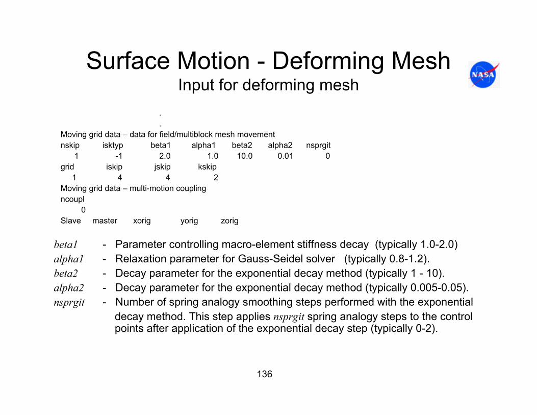
136
Surface Motion - Deforming MeshInput for deforming mesh
.
.Moving grid data – data for field/multiblock mesh movementnskip isktyp beta1 alpha1 beta2 alpha2 nsprgit
1 -1 2.0 1.0 10.0 0.01 0grid iskip jskip kskip
1 4 4 2Moving grid data – multi-motion couplingncoupl
0Slave master xorig yorig zorig
beta1 - Parameter controlling macro-element stiffness decay (typically 1.0-2.0)alpha1 - Relaxation parameter for Gauss-Seidel solver (typically 0.8-1.2).beta2 - Decay parameter for the exponential decay method (typically 1 - 10).alpha2 - Decay parameter for the exponential decay method (typically 0.005-0.05).nsprgit - Number of spring analogy smoothing steps performed with the exponential
decay method. This step applies nsprgit spring analogy steps to the control points after application of the exponential decay step (typically 0-2).

137
Surface Motion - Deforming MeshInput for deforming mesh
• There are 4 options for the construction of control points.– Option 1: Code generated minimum number of control points.– Option 2: Code generated default skip values.– Option 3: User input of i,j,k skip values for each block. – Option 4: User defined input of control point i,j,k indices for each block.
• These options depend on the value of nskip and the value of isktyp– Option 1: isktyp = -2, 2 and nskip = 0– Option 2: isktyp = -1, 1 and nskip = 0 – Option 3: isktyp = -1, 1 and nskip = ngrid (Note: ngrid = number of grid blocks)– Option 4: isktyp = -2, 2 and nskip = ngrid
• Option 1 creates the minimum number of control points (at non-constant intervals) by placing control point points only at each boundary segment extremity. This is the preferred method.
• Options 2 creates skip values that result in control points at constant intervals through out each of the grids, with control points at each boundary segment extremity. Sometimes this is more robust than option 1, but can create many more control points.
preferredmethod
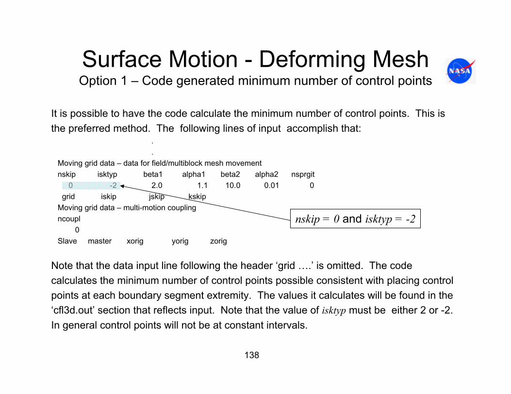
138
Surface Motion - Deforming MeshOption 1 – Code generated minimum number of control points
It is possible to have the code calculate the minimum number of control points. This is the preferred method. The following lines of input accomplish that:
.
.Moving grid data – data for field/multiblock mesh movementnskip isktyp beta1 alpha1 beta2 alpha2 nsprgit
0 -2 2.0 1.1 10.0 0.01 0grid iskip jskip kskip
Moving grid data – multi-motion couplingncoupl
0Slave master xorig yorig zorig
Note that the data input line following the header ‘grid ….’ is omitted. The code calculates the minimum number of control points possible consistent with placing control points at each boundary segment extremity. The values it calculates will be found in the ‘cfl3d.out’ section that reflects input. Note that the value of isktyp must be either 2 or -2.In general control points will not be at constant intervals.
nskip = 0 and isktyp = -2

139
Surface Motion - Deforming MeshOption 2 – Code generated skip values
It is possible to have the code calculate default skip values. The following lines of input accomplish that:
.
.Moving grid data – data for field/multiblock mesh movementnskip isktyp beta1 alpha1 beta2 alpha2 nsprgit
0 -1 2.0 1.1 10.0 0.01 0grid iskip jskip kskip
Moving grid data – multi-motion couplingncoupl
0Slave master xorig yorig zorig
Note that the data input line following the header ‘grid ….’ is omitted. The code calculates the largest values of iskip, jskip, kskip possible. The values it calculates will be found in the ‘cfl3d.out’ section that reflects input. Note that the value of isktyp must be either 1 or -1.
nskip = 0 and isktyp = -1
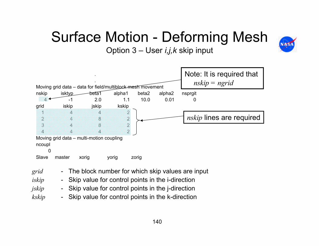
140
Surface Motion - Deforming MeshOption 3 – User i,j,k skip input
.
.Moving grid data – data for field/multiblock mesh movementnskip isktyp beta1 alpha1 beta2 alpha2 nsprgit
4 -1 2.0 1.1 10.0 0.01 0grid iskip jskip kskip
1 4 4 22 4 8 23 4 8 24 4 4 2
Moving grid data – multi-motion couplingncoupl
0Slave master xorig yorig zorig
grid - The block number for which skip values are inputiskip - Skip value for control points in the i-direction jskip - Skip value for control points in the j-directionkskip - Skip value for control points in the k-direction
nskip lines are required
Note: It is required that nskip = ngrid
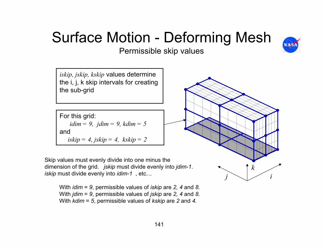
141
kj i
Surface Motion - Deforming MeshPermissible skip values
For this grid: idim = 9, jdim = 9, kdim = 5
andiskip = 4, jskip = 4, kskip = 2
iskip, jskip, kskip values determinethe i, j, k skip intervals for creating the sub-grid
Skip values must evenly divide into one minus the dimension of the grid. jskip must divide evenly into jdim-1. iskip must divide evenly into idim-1 , etc…
With idim = 9, permissible values of iskip are 2, 4 and 8.With jdim = 9, permissible values of jskip are 2, 4 and 8.With kdim = 5, permissible values of kskip are 2 and 4.
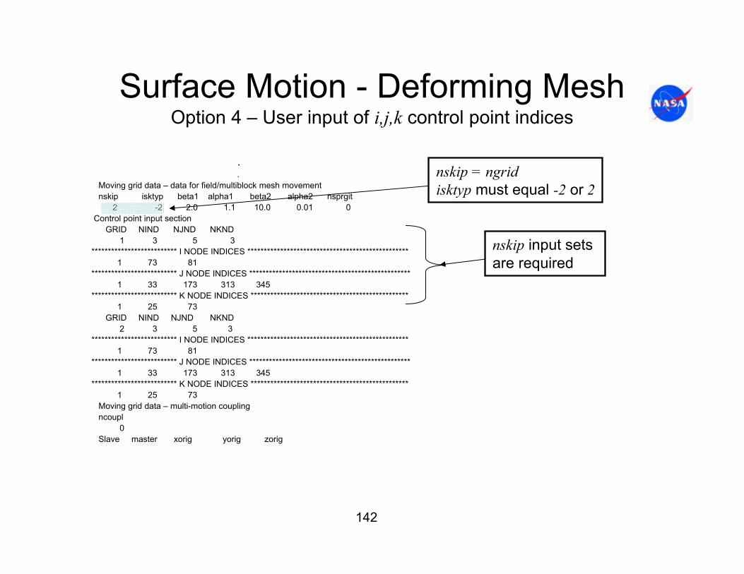
142
Surface Motion - Deforming MeshOption 4 – User input of i,j,k control point indices
.
.Moving grid data – data for field/multiblock mesh movementnskip isktyp beta1 alpha1 beta2 alpha2 nsprgit
2 -2 2.0 1.1 10.0 0.01 0Control point input section
GRID NIND NJND NKND1 3 5 3
************************** I NODE INDICES *************************************************1 73 81
************************** J NODE INDICES *************************************************1 33 173 313 345
************************** K NODE INDICES ************************************************1 25 73
GRID NIND NJND NKND2 3 5 3
************************** I NODE INDICES *************************************************1 73 81
************************** J NODE INDICES *************************************************1 33 173 313 345
************************** K NODE INDICES ************************************************1 25 73
Moving grid data – multi-motion couplingncoupl
0Slave master xorig yorig zorig
nskip input sets are required
nskip = ngridisktyp must equal -2 or 2

143
Surface Motion - Deforming MeshOption 4 – User input of i,j,k control point indices
• This option is used when there are problem areas in the surface motion that require customized control point placement. e.g. significant surface motion restricted to a small portion of the entire surface area or if the finite macro-elementmethod is used and added control points are needed to define affine element shapes.
• Note that a control point must be placed at the extremities of all boundary condition segments, 1-1 blocking segments and all block corners.
• The code will do a check at 1-1 blocking segments to see if the control points youhave selected result in continuity in control placement between 1-1 blocking boundaries. It will add points as necessary to maintain control point continuity. Thisis a very powerful feature that can be very useful when adding control points.
• The code will not tell you if a b.c. segment extremity or block corner does not have a control point assigned to it. It will simply cause the grid motion to be messed up and produce negative volumes!

144
Surface Motion - Deforming MeshExample 1: 3D Control surface rotation with exponential decay method
x
z y
Trailing edge controlsurface
As an example consider the wing shown undergoing control surface rotation:

145
Surface Motion - Deforming MeshExample 1: 3D Control surface rotation with exponential decay method
The following unsteady input file performs the control surface rotation about the hinge point:input/output files:
wbgrid.cflplot3dg.bin plot3dq.bin cfl3d.out cfl3d.rescfl3d.turres cfl3d.blomaxcfl3d.out15 cfl3d.prout cfl3d.out20 ovrlp.binpatch.binrestart.bin
NASA Langley BACT Model: NACA 0012 af, AR=1.5 wing,.75TE FlapMach alpha beta ReUe Tinf,dR ialph ihstry
0.82000 0.00000 0.00000 0.236E+07 486.00 1 0sref cref bref xmc ymc zmc
1.000 1.00000 1.00000 0.25000 0.00000 0.00000dt irest iflagts fmax iunst cfl_tau
0.04000 0 3000 1.00000 2 2.00000ngrid nplot3d nprint nwrest ichk i2d ntstep ita
1 1 1 1000 0 0 1 -2
Note that iunst = 2 for deforming mesh

146
Surface Motion - Deforming MeshExample 1: 3D Control surface rotation with exponential decay method
ncg iem iadvance iforce ivisc(i) ivisc(j) ivisc(k)2 0 0 1 5 5 5
idim jdim kdim81 345 73
ilamlo ilamhi jlamlo jlamhi klamlo klamhi0 0 0 0 0 0
inewg igridc is js ks ie je ke0 0 0 0 0 0 0 0
idiag(i) idiag(j) idiag(k) iflim(i) iflim(j) iflim(k)1 1 1 4 4 4
ifds(i) fds(j) ifds(k) rkap0(i) rkap0(j) rkap0(k)1 1 1 0.3333 0.3333 0.3333
grid nbci0 nbcidim nbcj0 nbcjdim nbck0 nbckdim iovrlp1 1 1 1 1 5 1 0
i0: grid segment bctype jsta jend ksta kend ndata1 1 1005 1 345 1 73 0
idim: grid segment bctype jsta jend ksta kend ndata1 1 1002 1 345 1 73 0
j0: grid segment bctype ista iend ksta kend ndata1 1 1003 1 81 1 73 0
jdim: grid segment bctype ista end ksta kend ndata1 1 1003 1 81 1 73 0
k0: grid segment bctype ista iend jsta jend ndata1 1 0 1 73 1 33 01 2 2004 1 73 33 313 2
tw/tinf cq0.00000 0.00000
1 3 0 1 73 313 345 01 4 0 73 81 1 173 01 5 0 73 81 173 345 0
kdim: grid segment bctype ista iend jsta jend ndata 1 1 1003 1 81 1 345 0
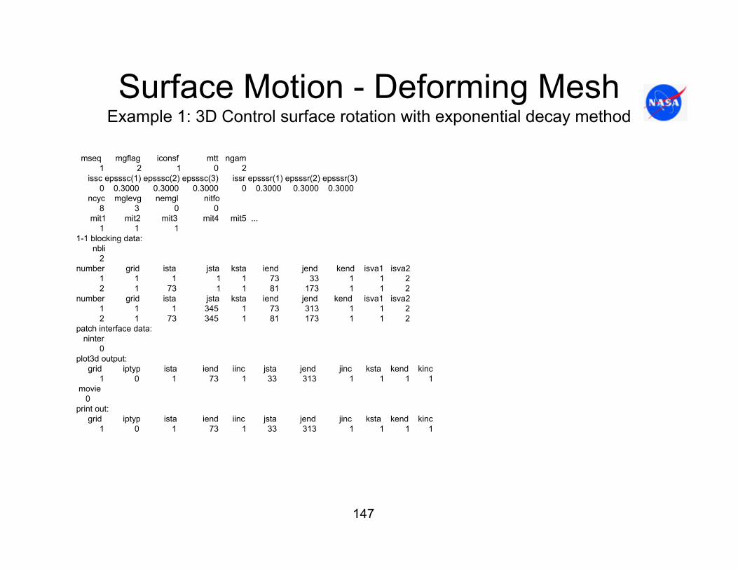
147
Surface Motion - Deforming MeshExample 1: 3D Control surface rotation with exponential decay method
mseq mgflag iconsf mtt ngam1 2 1 0 2
issc epsssc(1) epsssc(2) epsssc(3) issr epsssr(1) epsssr(2) epsssr(3)0 0.3000 0.3000 0.3000 0 0.3000 0.3000 0.3000
ncyc mglevg nemgl nitfo8 3 0 0
mit1 mit2 mit3 mit4 mit5 ...1 1 1
1-1 blocking data:nbli
2number grid ista jsta ksta iend jend kend isva1 isva2
1 1 1 1 1 73 33 1 1 22 1 73 1 1 81 173 1 1 2
number grid ista jsta ksta iend jend kend isva1 isva21 1 1 345 1 73 313 1 1 2 2 1 73 345 1 81 173 1 1 2
patch interface data:ninter
0plot3d output:
grid iptyp ista iend iinc jsta jend jinc ksta kend kinc1 0 1 73 1 33 313 1 1 1 1
movie0
print out:grid iptyp ista iend iinc jsta jend jinc ksta kend kinc
1 0 1 73 1 33 313 1 1 1 1

148
Surface Motion - Deforming MeshExample 1: 3D Control surface rotation with exponential decay method
Control Surfaces:ncs0
Grid ista iend jsta jend ksta kend iwall inormMoving grid data – deforming surface (forced motion):ndefrm
2lref1.0
Grid idefrm rfreq u/omegax v/omegay w/omegaz xorig yorig zorig1 2 0.05 0.00 5.00 0.00 0.75 0.00 0.001 2 0.05 0.00 5.00 0.00 0.75 0.00 0.00
Grid icsi icsf jcsi jcsf kcsi kcsf1 29 53 33 72 1 1 1 29 53 274 313 1 1
Moving grid data – aeroelastic surface (aeroelastic motion):naesrf
0Iaesrf ngrid grefl uinf qinf nmodes iskyhookFreq gmass damp x0(2n-1) xo(2n) gf0(2n)
Moddfl amp freq t0Grid iaei iaef jaei jaef kaei kaef
Moving grid data – data for field/multiblock mesh movementnskip isktyp beta1 alpha1 beta2 alpha2 nsprgit
0 -2 1.0 1.1 1.0 0.005 0Control point index input
Moving grid data – multi-motion couplingncoupl
0Slave master xorig yorig zorig
The following lines mustbe included when iunst = 2
User specified surfacemotion input
Aeroelasticity input. Notethat only header cards are input when naesrf = 0
Mesh deformation input

149
.
.Moving grid data – deforming surface (forced motion):ndefrm
2lref1.0
Grid idefrm rfreq u/omegax v/omegay w/omegaz xorig yorig zorig1 2 0.05 0.00 5.00 0.00 0.75 0.00 0.001 2 0.05 0.00 5.00 0.00 0.75 0.00 0.00
Grid icsi icsf jcsi jcsf kcsi kcsf1 29 53 33 72 1 1 1 29 53 274 313 1 1
.
.
Grid - grid block containing the moving surfaceidefrm - type of surface motion
= 1 - translation= 2 - rotation
rfreq - reduced frequency of the surface motion
u/omegax, v/omegay, w/omegaz - x,y,z-components of surface translational velocity if idefrm = 1- x,y,z-components of surface rotational velocity if idefrm = 2
xorig, yorig, zorig - x,y,z coordinates of the origin of the rotation axis (note: value must be input even when idefrm = 1)
Surface Motion - Deforming MeshExample 1: 3D Control surface rotation with exponential decay method
ndefrm lines required
ndefrm lines required
Note that ndefrm = 2 because the trailing edge control surface is defined by an upper wing surface segment and a lower wing surface segment
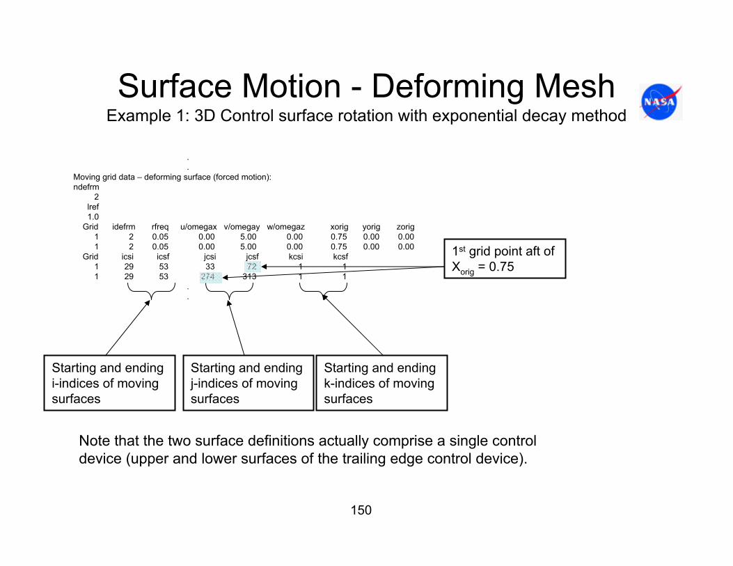
150
Surface Motion - Deforming MeshExample 1: 3D Control surface rotation with exponential decay method
.
.Moving grid data – deforming surface (forced motion):ndefrm
2lref1.0
Grid idefrm rfreq u/omegax v/omegay w/omegaz xorig yorig zorig1 2 0.05 0.00 5.00 0.00 0.75 0.00 0.001 2 0.05 0.00 5.00 0.00 0.75 0.00 0.00
Grid icsi icsf jcsi jcsf kcsi kcsf1 29 53 33 72 1 1 1 29 53 274 313 1 1
.
.
Starting and ending i-indices of moving surfaces
Starting and ending j-indices of moving surfaces
Starting and ending k-indices of moving surfaces
Note that the two surface definitions actually comprise a single control device (upper and lower surfaces of the trailing edge control device).
1st grid point aft of Xorig = 0.75
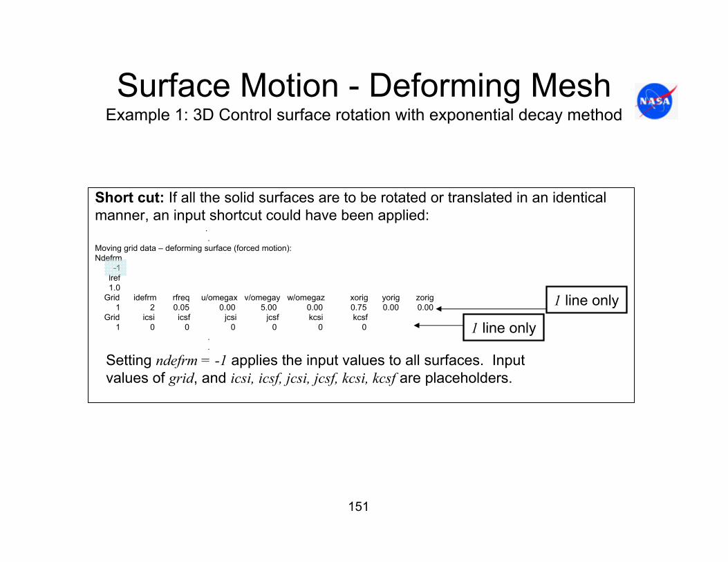
151
Surface Motion - Deforming MeshExample 1: 3D Control surface rotation with exponential decay method
Short cut: If all the solid surfaces are to be rotated or translated in an identical manner, an input shortcut could have been applied:
..
Moving grid data – deforming surface (forced motion):Ndefrm
-1lref1.0
Grid idefrm rfreq u/omegax v/omegay w/omegaz xorig yorig zorig1 2 0.05 0.00 5.00 0.00 0.75 0.00 0.00
Grid icsi icsf jcsi jcsf kcsi kcsf1 0 0 0 0 0 0
.
.
1 line only
1 line only
Setting ndefrm = -1 applies the input values to all surfaces. Inputvalues of grid, and icsi, icsf, jcsi, jcsf, kcsi, kcsf are placeholders.

152
Surface Motion - Deforming MeshExample 1: 3D Control surface rotation with exponential decay method
Moving grid data – data for field/multiblock mesh movementnskip isktyp beta1 alpha1 beta2 alpha2 nsprgit
0 -2 1.0 1.1 1.0 0.005 0Control point index input
Note that α2 * ∆ rmax is the distance to whichsurface motion is transmitted unabated intothe flow field
β2 - rate at which surface motion decaysaway from a moving surface (outside of inner region controlled by α2)
Control point index input using Exponential Decay Method (isktyp < 0)
nskip = 0 forces automatic generation of the minimum number of control points (with isktyp = -2,2) at all segment and block extremities, while maintaining continuity at all blocking boundaries

153
Surface Motion - Deforming MeshExample 1: 3D Control surface rotation with exponential decay method
Moving grid data – data for field/multiblock mesh movementnskip isktyp beta1 alpha1 beta2 alpha2 nsprgit
0 -2 2.0 1.1 1.0 0.005 0Control point index input
Moving grid data – multi-motion couplingncoupl
0Slave master xorig yorig zorig
• This input option automatically creates the following control points: (This format is how it would look if you were to input these control points by hand (i.e. using Option 4))
• Note that i node indices, j node indices, k node indices span the entire block. (i.e. idim = 81, jdim = 345, kdim = 73)
• Boundary segments have a control point. The trailing edge at j = 33 and 313has control points assigned. The wing tip at i = 73 has a control point assigned.
• Other control points have been assigned at discontinuities in the surface movement.(e.g. at i = 28, 29 and 53, 54 and j = 72, 73 and 273, 274) See the next slide.
GRID NIND NJND NKND1 7 8 2
************************** I NODE INDICES *************************************************1 28 29 53 54 73 81
************************** J NODE INDICES *************************************************1 33 72 73 273 274 313 345
************************** K NODE INDICES ************************************************1 73
Control point option 1 is used here

154
Surface Motion - Deforming MeshExample 1: 3D Control surface rotation with exponential decay method
Upper surface control point locations
GRID NIND NJND NKND1 7 8 3
************************** I NODE INDICES *************************************************1 28 29 53 54 73 81
************************** J NODE INDICES *************************************************1 33 72 73 273 274 313 345
************************** K NODE INDICES ************************************************1 25 73
Control points selectedCenter of rotation
Discontinuous grid motion
Control surface definition
Control pointslocated at allgrid motiondiscontinuities
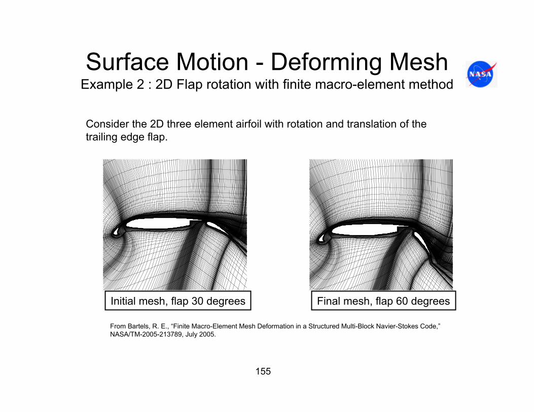
155
Surface Motion - Deforming MeshExample 2 : 2D Flap rotation with finite macro-element method
Consider the 2D three element airfoil with rotation and translation of the trailing edge flap.
Final mesh, flap 60 degrees
From Bartels, R. E., “Finite Macro-Element Mesh Deformation in a Structured Multi-Block Navier-Stokes Code,”NASA/TM-2005-213789, July 2005.
Initial mesh, flap 30 degrees

156
Surface Motion - Deforming MeshExample 2 : 2D Flap rotation with finite macro-element method
.
.MOVING GRID DATA - DEFORMING SURFACE (FORCED MOTION):NDEFRM
1LREF
1.0GRID IDEFRM RFREQ U/OMEGAX V/OMEGAY W/OMEGAZ XORIG YORIG ZORIG
3 2 0.05 0.00 25.00 0.00 0.80 0.00 0.00GRID ICSI ICSF JCSI JCSF KCSI KCSF
3 1 2 49 217 1 1MOVING GRID DATA - AEROELASTIC SURFACE (AEROELASTIC MOTION):NAESRF
0IAESRF NGRID GREFL UINF QINF NMODES ISKYHOKFREQ GMASS DAMP X0(2N-1) X0(2N) GF0(2N)
MODDFL AMP FREQ T0GRID IAEI IAEF JAEI JAEF KAEI KAEF
MOVING GRID DATA - DATA FOR FIELD/MULTIBLOCK MESH MOVEMENTNSKIP ISKTYP BETA1 ALPHA1 BETA2 ALPHA2 ISPRNIT
4 2 1.000 1.000 20.000 0.005 0CONTROL POINT INDEX INPUT
GRID NIND NJND NKND1 2 33 2
********************************************* I NODE INDICES **************************************************1 2
Number of meshblocks
This section definesthe rotation of thetrailing edge flap
Finite Macro-ElementMethod with user inputof control point indices
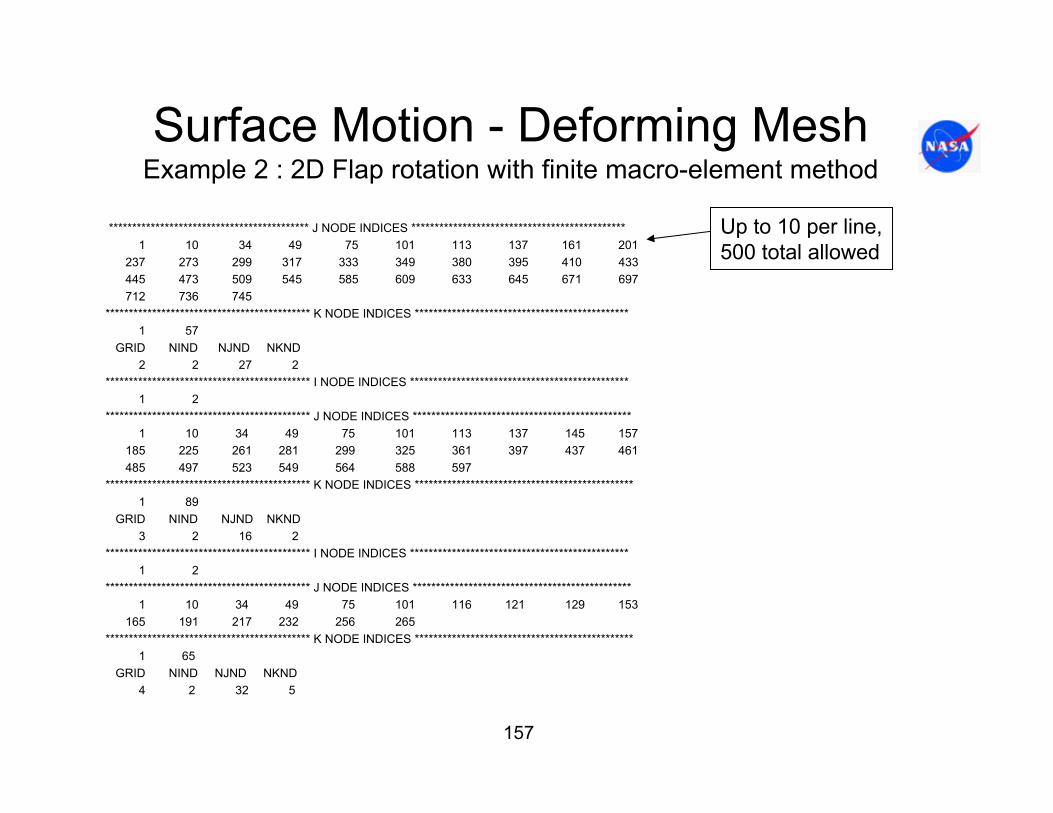
157
Surface Motion - Deforming MeshExample 2 : 2D Flap rotation with finite macro-element method
******************************************* J NODE INDICES **********************************************1 10 34 49 75 101 113 137 161 201
237 273 299 317 333 349 380 395 410 433445 473 509 545 585 609 633 645 671 697712 736 745
******************************************** K NODE INDICES **********************************************1 57
GRID NIND NJND NKND2 2 27 2
******************************************** I NODE INDICES ***********************************************1 2
******************************************** J NODE INDICES ***********************************************1 10 34 49 75 101 113 137 145 157
185 225 261 281 299 325 361 397 437 461485 497 523 549 564 588 597
******************************************** K NODE INDICES ***********************************************1 89
GRID NIND NJND NKND3 2 16 2
******************************************** I NODE INDICES ***********************************************1 2
******************************************** J NODE INDICES ***********************************************1 10 34 49 75 101 116 121 129 153
165 191 217 232 256 265******************************************** K NODE INDICES ***********************************************
1 65GRID NIND NJND NKND
4 2 32 5
Up to 10 per line,500 total allowed

158
Surface Motion - Deforming MeshExample 2 : 2D Flap rotation with finite macro-element method
******************************************* I NODE INDICES *********************************************1 2
******************************************* J NODE INDICES *********************************************1 10 34 49 75 101 116 121 133 161
201 237 257 273 289 320 335 350 373 385413 449 485 525 549 573 585 611 637 652676 685
******************************************* K NODE INDICES *********************************************1 10 17 24 33
MOVING GRID DATA - MULTI-MOTION COUPLINGNCOUPL
0SLAVE MASTER XORIG YORIG ZORIG
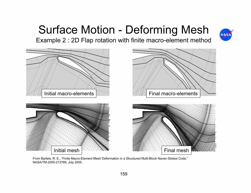
159
Surface Motion - Deforming MeshExample 2 : 2D Flap rotation with finite macro-element method
From Bartels, R. E., “Finite Macro-Element Mesh Deformation in a Structured Multi-Block Navier-Stokes Code,”NASA/TM-2005-213789, July 2005.
Initial macro-elements Final macro-elements
Initial mesh Final mesh
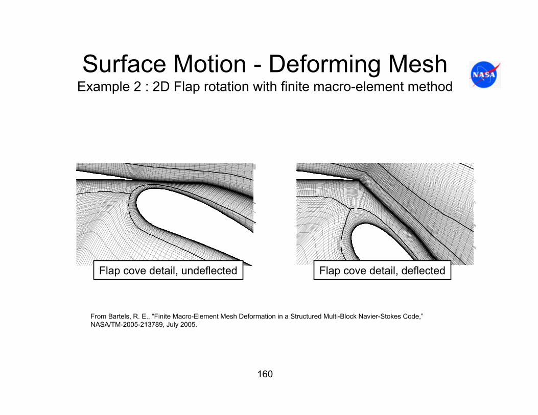
160
Surface Motion - Deforming MeshExample 2 : 2D Flap rotation with finite macro-element method
From Bartels, R. E., “Finite Macro-Element Mesh Deformation in a Structured Multi-Block Navier-Stokes Code,”NASA/TM-2005-213789, July 2005.
Flap cove detail, undeflected Flap cove detail, deflected

161
Surface Motion - Deforming MeshExample 2 : 2D Flap rotation – 1-1 block point checking
Control points without 1-1 point blocking check
Control points with 1-1 point blocking check
Control point orientation after flap is deflected
Block boundariesseparate due to high strain rates in coveregion.
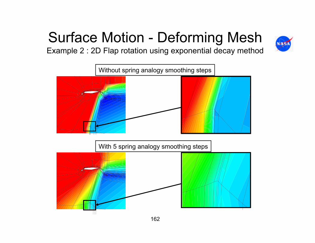
162
Surface Motion - Deforming MeshExample 2 : 2D Flap rotation using exponential decay method
Without spring analogy smoothing steps
With 5 spring analogy smoothing steps

163
Surface Motion - Deforming MeshExample 2 : 2D Flap rotation using exponential decay method
.
.MOVING GRID DATA - DATA FOR FIELD/MULTIBLOCK MESH MOVEMENT
NSKIP ISKTYP BETA1 ALPHA1 BETA2 ALPHA2 ISPRNIT0 -2 1.000 1.100 2.000 0.05 2
CONTROL POINT INDEX INPUTMOVING GRID DATA - MULTI-MOTION COUPLINGNCOUPL
0SLAVE MASTER XORIG YORIG ZORIG
An alternate approach is to allow automatic creation of the minimum numberof control points. (Option 1) The input below accomplishes that by setting nskip = 0. Note that the exponential decay method is used (isktyp < 0).
These parameters define thecontrol point motion with the Exponential Decay Method

164
Surface Motion - Deforming MeshExample 2 : 2D Flap rotation using exponential decay method
.
.moving grid data - data for field/multiblock mesh movement
nskip isktyp beta1 alpha1 beta2 alpha2 nsprngit4 -2 1.000000 1.100000 2.000000 0.050000 2
ng nipt njpt nkpt1 2 11 2
control point i-indices for grid levels 1 2 31 1 12 1 1
control point j-indices for grid levels 1 2 31 1 1
49 25 1350 25 13
137 69 35273 137 69317 159 80473 237 119609 305 153696 348 174697 349 175745 373 187
control point k-indices for grid levels 1 2 31 1 1
57 29 15
The control points that are code selected appear in the ‘cfl3d.out’ file:
ng nipt njpt nkpt2 2 11 2
control point i-indices for grid levels 4 5 61 1 1 2 1 1
control point j-indices for grid levels 4 5 61 1 1
49 25 1350 25 13
137 69 35145 73 37281 141 71325 163 82461 231 116548 274 137549 275 138597 299 150
control point k-indices for grid levels 4 5 61 1 1
89 45 23...
The resulting mesh movement is shown in the next slide.
Control pointsat finest grid level
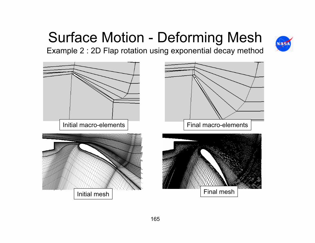
165
Surface Motion - Deforming MeshExample 2 : 2D Flap rotation using exponential decay method
Initial macro-elements Final macro-elements
Initial mesh Final mesh

166
Surface Motion - Deforming MeshExample 2 : 2D Flap rotation
• The mesh movement shown in the previous slides is robust (no negative volumes) through the entire range of motion shown, however mesh quality aft of the flap is somewhat degraded afterdeflection.
• If β2 is set to 1.0 or if the finite macro-element method is used with the code selected minimum number of control points (as was shown), negative volumes are the result.
• There is a simple way to fix this problem, demonstrated next. In the process an option for running the code will be demonstrated in which only the mesh motion and mesh calculations (e.g. metric and volume calculations) are performed in the code. This option greatly speeds up the code when the mesh motion is being debugged.
• The ‘Mesh only’ run option is invoked by using the keyword input, meshdef 1 . Keyword input will be discussed in detail later in the course. Note spelling and capitalization are important.
• The input to accomplish this is as follows:..
cfl3d.out20 ovrlp.binpatch.binrestart.bin
>meshdef 1negvol 1<3 Element Airfoil case
Mach alpha beta ReUe Tinf,dR ialph ihstry..
Keyword input

167
Surface Motion - Deforming MeshExample 2 : 2D Flap rotation
• Setting the keyword meshdef to 1 also causes the control points to be output in a Tecplot file in point wise data format. Other auxiliary data are also printed out in other files.
• If one processor is used all block control points are output into the file Tecplot datafile ‘fort.4000’. Data included in this file are x,y,z locations of control points, x,y,zdeflections per time step, node number, and node number of the nearest surface point.
• If multiple processors are used, the control points from the blocks processed on each processor are put in the successive files ‘fort.4001, fort.4002, …’
• Note that if the option movie = inc is used, the control points at every inc time steps will be output. If movie = 0, only control points at the final time step will be output.
• Once the control points are plotted it is possible to better visualize where added control points need to be placed.
• This is the option that was used to create the plots of control points shown in this presentation.

168
Surface Motion - Deforming MeshExample 2 : 2D Flap rotation
• Returning to the flap rotation example above, say we want to run it using control pointoption 1 (nskip = 0, isktyp = -2,2) but now using the finite macro-element method(isktyp = 2)
• The input parameters used are: β1 = 1.0, α1 = 0.9.• Keywords ‘meshdef 1’ and ‘negvol 1’ are set. When the keyword ‘negvol 1’ is used,
the code continues executing and prints a diagnostic message in ‘cfl3d.out’ indicating where the negative volume occurred.
• The code encounters negative volumes, with the following messages appearing in the ‘cfl3d.out’ file:
.
.WARNING ... negative volume at i,j,k= 1 514 2 block 1 not stopping!WARNING ... negative volume at i,j,k= 1 515 2 block 1 not stopping!
.
.• The majority of negative volumes appear to be in block 1. By plotting the control point
output it is clear that elements around the leading edge slat are not well defined, and probably causing poorly defined (singular) macro-elements in that region.

169
Surface Motion - Deforming MeshExample 2 : 2D Flap rotation
• The first step in solving this problem is to observe that the file ‘meshdef.inp’has been created.
• This file contains the control points that were created by the code.
• Contents of this file can be pasted into the input and customized as needed.
• Since negative volumes occurred in block 1 we will add to the control points in that block.
GRID NIND NJND NKND1 2 11 2
******************************* I NODE INDICES ************************************1 2
******************************* J NODE INDICES ***********************************1 49 50 137 273 317 473 609 696 697
745******************************* K NODE INDICES ***********************************
1 57GRID NIND NJND NKND
2 2 11 2******************************* I NODE INDICES ************************************
1 2******************************* J NODE INDICES ************************************
1 49 50 137 145 281 325 461 548 549597
******************************* K NODE INDICES ***********************************1 89
GRID NIND NJND NKND3 2 8 2
******************************* I NODE INDICES ***********************************1 2
******************************* J NODE INDICES **********************************1 49 50 121 129 216 217 265
******************************* K NODE INDICES *********** ***********************1 65
GRID NIND NJND NKND4 2 10 2
******************************* I NODE INDICES ***********************************1 2
******************************* J NODE INDICES **********************************1 49 50 121 257 413 549 636 637 685
******************************* K NODE INDICES **********************************1 33
Contents of ‘meshdef.inp’:

170
Surface Motion - Deforming MeshExample 2 : 2D Flap rotation
• These additional points have been chosen simply to fill in gaps in the control point distribution.
• This customized input is pasted into the input file, and nskip set to 4.
GRID NIND NJND NKND1 2 18 2
******************************* I NODE INDICES ************************************1 2
******************************* J NODE INDICES ***********************************1 49 50 103 137 173 223 273 297 317
373 423 473 543 609 696 697 745******************************* K NODE INDICES ***********************************
1 57GRID NIND NJND NKND
2 2 11 2******************************* I NODE INDICES ************************************
1 2******************************* J NODE INDICES ************************************
1 49 50 137 145 281 325 461 548 549597
******************************* K NODE INDICES ***********************************1 89
GRID NIND NJND NKND3 2 12 2
******************************* I NODE INDICES ***********************************1 2
******************************* J NODE INDICES **********************************1 49 50 73 101 121 129 137 157 216
217 265******************************* K NODE INDICES *********** ***********************
1 65GRID NIND NJND NKND
4 2 10 4******************************* I NODE INDICES ***********************************
1 2******************************* J NODE INDICES **********************************
1 49 50 121 257 413 549 636 637 685******************************* K NODE INDICES **********************************
1 10 17 33
Contents of ‘meshdef.inp’ customized:
Points added that remove the negative volumes in block 1
Points added to better definethe flap region

171
GRID NIND NJND NKND1 2 26 2
********************************** I NODE INDICES ************************************ 1 2
********************************** J NODE INDICES ************************************1 49 50 103 109 129 137 173 203 223
273 297 317 373 423 473 523 543 573 609617 637 643 696 697 745
********************************** K NODE INDICES ************************************1 57
GRID NIND NJND NKND....
GRID NIND NJND NKND3 2 13 2
********************************** I NODE INDICES *************************************1 2
********************************** J NODE INDICES *************************************1 49 50 73 101 121 129 137 157 163
216 217 265********************************** K NODE INDICES ************************************
1 65GRID NIND NJND NKND
4 2 20 4********************************** I NODE INDICES ************************************
1 2********************************** J NODE INDICES ************************************
1 49 50 73 101 121 257 313 363 413463 483 513 549 557 577 583 636 637 685
********************************** K NODE INDICES ************************************1 10 17 33
Surface Motion - Deforming MeshExample 2 : 2D Flap rotation
This is the data output into the new file ‘meshdef.inp’ after the code is rerun. This file is printed out because new points have been added by the codein addition to points added by the user.
Control points added by user
Control points added by the code to maintain 1-1 blocking interfacecontinuity
Control point indices the code actually uses:

172
Surface Motion - Deforming MeshExample 2 : 2D Flap rotation
Control point lines added by the user
Control point indices the code actually uses:
With these new control points, the code runs robustly with no negativevolumes for both the exponential decay and finite macro-element methodsfor a range of parameter values. Note that the region just aft of the flap retains grid quality better using the finite macro-element method than did the original.
Control point lines addedby the code to maintaincontinuity at 1-1 blockinginterfaces

173
Surface Motion - Deforming MeshExample 3 : 2D airfoil rotation with finite macro-element method
From Bartels, R. E., “Finite Macro-Element Mesh Deformation in a Structured Multi-Block Navier-Stokes Code,”NASA/TM-2005-213789, July 2005.
Initial macro-element orientation Finite macro-element orientationafter pitch up
Trailing edge detail of macro-element Orientation – note orthogonality
Trailing edge detail of mesh orientation
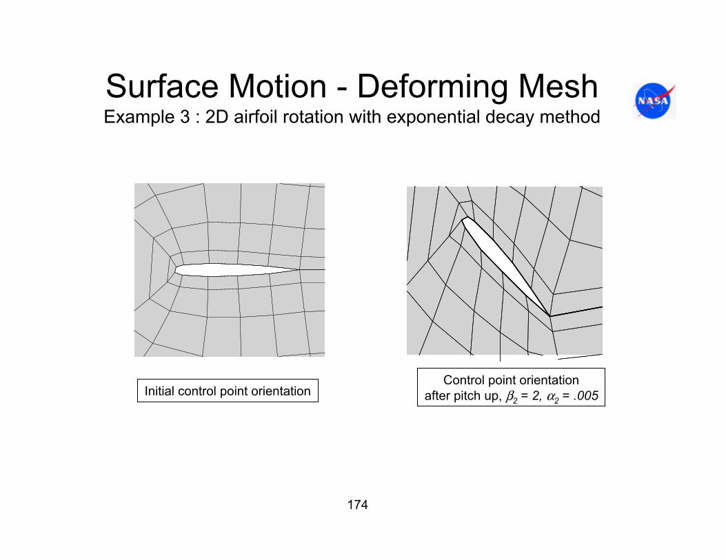
174
Surface Motion - Deforming MeshExample 3 : 2D airfoil rotation with exponential decay method
Initial control point orientationControl point orientation
after pitch up, β2 = 2, α2 = .005
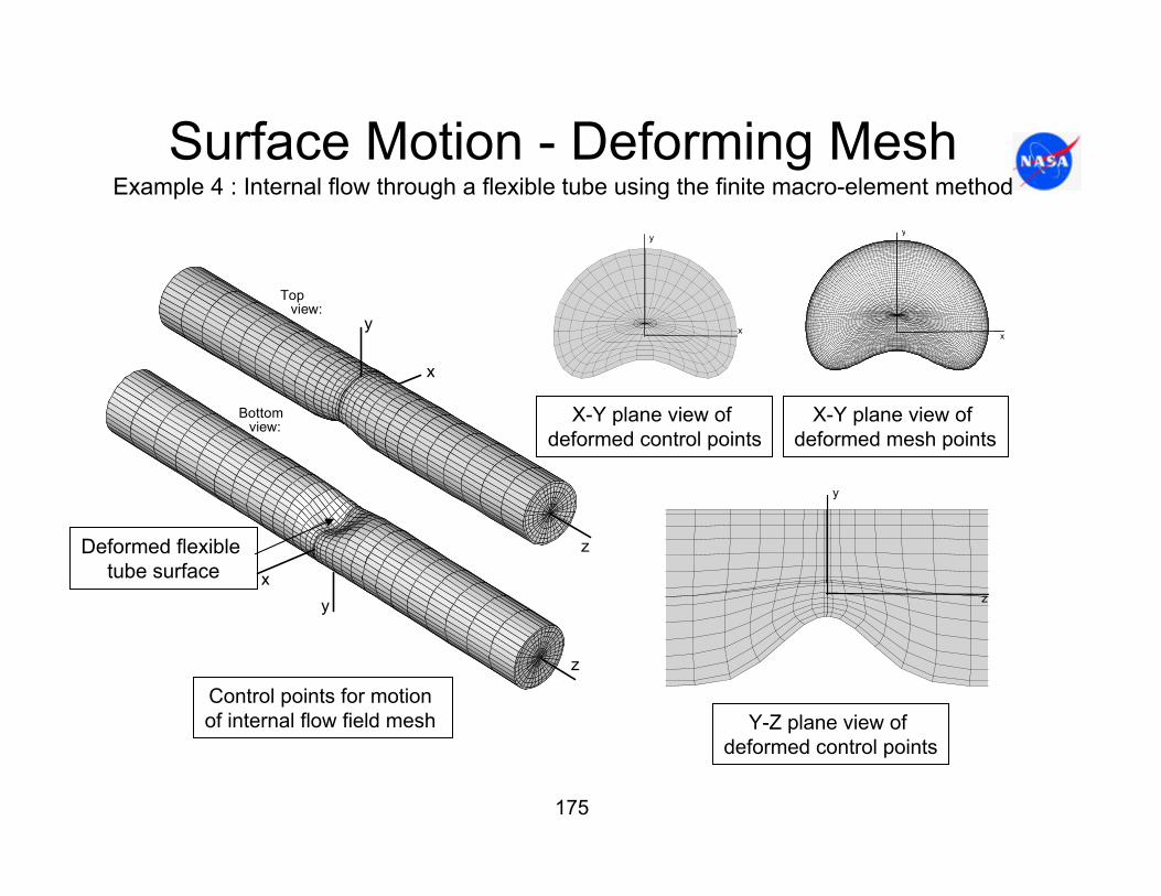
175
Surface Motion - Deforming MeshExample 4 : Internal flow through a flexible tube using the finite macro-element method
y
x
z
xy
z
Topview:
Bottomview:
y
x
y
z
y
x
X-Y plane view of deformed control points
X-Y plane view of deformed mesh points
Y-Z plane view of deformed control points
Control points for motion of internal flow field mesh
Deformed flexible tube surface

176
Surface Motion - Deforming MeshExample 5 : Transport wing bending using the Exponential Decay Method
Deformed mesh
Initial and deformed geometry
This example used mesh movement Option 2 (isktyp = -1, nskip = 0)
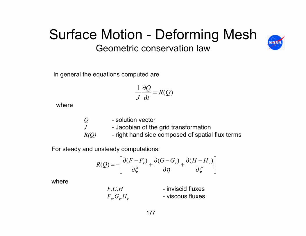
177
Surface Motion - Deforming MeshGeometric conservation law
In general the equations computed are
)(1 QRtQ
J=
∂∂
where
Q - solution vectorJ - Jacobian of the grid transformationR(Q) - right hand side composed of spatial flux terms
For steady and unsteady computations:
⎥⎦
⎤⎢⎣
⎡∂−∂+
∂−∂+
∂−∂−=
ζηξ)()()()( vvv HHGGFFQR
whereF,G,H - inviscid fluxesFv,Gv,Hv - viscous fluxes

178
Surface Motion - Deforming MeshGeometric conservation law
For unsteady deforming mesh computations there is an additional term:
⎥⎦
⎤⎢⎣
⎡⎟⎠⎞
⎜⎝⎛
∂∂+⎟
⎠⎞
⎜⎝⎛
∂∂+⎟
⎠⎞
⎜⎝⎛
∂∂+⎟
⎠⎞
⎜⎝⎛
∂∂+
⎥⎦
⎤⎢⎣
⎡∂−∂+
∂−∂+
∂−∂−=
JJJJtQ
HHGGFFQR
ttt
vvv
ζζ
ηη
ξξ
ζηξ
1
)()()()(
Geometric Conservation Law (GCL), due to grid volumechange
The implication of this is that a computation using rigid grid motion mayperform somewhat differently than a deforming grid solution with the same time step size, number of sub-iterations and CFL number. However, the two fully converged solutions will be the same. See Bartels, R. E., “Mesh and Solution Strategies and the Accurate Computation of Unsteady Spoiler and Aeroelastic Problems,” Journal of Aircraft, Vol. 37, No. 3, May 2000, pp. 521-529.

179
Surface Motion - Deforming MeshMultiple types of coupled motion
Consider the example of wing plunge combined with control surface rotation. Since the control surface rotation is about a point fixed on the larger moving wing surface, coupling of the two motions will be required. There are two ways to perform this coupled motion:
1. Coupling control surface rotation and wing translation combined using mesh deformation.
2. Coupling control surface rotation using mesh deformation with rigid grid translation.
Although these two approaches result in identical wing surface motion, off body grid motion will be much different.

180
Surface Motion - Deforming MeshExample: Control surface rotation plus wing plunging
x
z y
Trailing edge controlsurface
As an example consider the wing shown having both wing plunge pluscontrol surface rotation:

181
Surface Motion - Deforming MeshExample: Multi-motion using deforming mesh
The following unsteady input file performs the wing plunging with control surface rotation using deforming mesh:
input/output files: wbgrid.cflplot3dg.bin plot3dq.bin cfl3d.out cfl3d.rescfl3d.turres cfl3d.blomaxcfl3d.out15 cfl3d.prout cfl3d.out20 ovrlp.binpatch.binrestart.bin
NASA Langley BACT Model: NACA 0012 af, AR=1.5 wing,.75TE FlapMach alpha beta ReUe Tinf,dR ialph ihstry
0.82000 0.00000 0.00000 0.236E+07 486.00 1 0sref cref bref xmc ymc zmc
1.000 1.00000 1.00000 0.25000 0.00000 0.00000dt irest iflagts fmax iunst cfl_tau
0.04000 0 3000 1.00000 2 2.00000ngrid nplot3d nprint nwrest ichk i2d ntstep ita
1 1 1 1000 0 0 1 -2
Note that iunst = 2 since deforming mesh is used

182
Surface Motion - Deforming MeshExample: Multi-motion using deforming mesh
ncg iem iadvance iforce ivisc(i) ivisc(j) ivisc(k)2 0 0 1 5 5 5
idim jdim kdim73 345 73
ilamlo ilamhi jlamlo jlamhi klamlo klamhi0 0 0 0 0 0
inewg igridc is js ks ie je ke0 0 0 0 0 0 0 0
idiag(i) idiag(j) idiag(k) iflim(i) iflim(j) iflim(k)1 1 1 3 3 3
ifds(i) fds(j) ifds(k) rkap0(i) rkap0(j) rkap0(k)1 1 1 0.3333 0.3333 0.3333
grid nbci0 nbcidim nbcj0 nbcjdim nbck0 nbckdim iovrlp1 1 1 1 1 5 1 0
i0: grid segment bctype jsta jend ksta kend ndata1 1 1001 1 345 1 73 0
idim: grid segment bctype jsta jend ksta kend ndata1 1 1002 1 345 1 73 0
j0: grid segment bctype ista iend ksta kend ndata1 1 1003 1 73 1 73 0
jdim: grid segment bctype ista end ksta kend ndata1 1 1003 1 73 1 73 0
k0: grid segment bctype ista iend jsta jend ndata1 1 0 1 49 1 33 01 2 2004 1 49 33 313 2
tw/tinf cq0.00000 0.00000
1 3 0 1 49 313 345 01 4 0 49 73 1 173 01 5 0 49 73 173 345 0
kdim: grid segment bctype ista iend jsta jend ndata 1 1 1003 1 73 1 345 0

183
Surface Motion - Deforming MeshExample: Multi-motion using deforming mesh
mseq mgflag iconsf mtt ngam1 2 1 0 2
issc epsssc(1) epsssc(2) epsssc(3) issr epsssr(1) epsssr(2) epsssr(3)0 0.3000 0.3000 0.3000 0 0.3000 0.3000 0.3000
ncyc mglevg nemgl nitfo8 3 0 0
mit1 mit2 mit3 mit4 mit5 ...1 1 1
1-1 blocking data:nbli
2number grid ista jsta ksta iend jend kend isva1 isva2
1 1 1 1 1 49 33 1 1 22 1 49 1 1 73 173 1 1 2
number grid ista jsta ksta iend jend kend isva1 isva21 1 1 345 1 49 313 1 1 2 2 1 49 345 1 73 173 1 1 2
patch interface data:ninter
0plot3d output:
grid iptyp ista iend iinc jsta jend jinc ksta kend kinc1 0 1 49 1 1 345 1 1 1 1
movie0
print out:grid iptyp ista iend iinc jsta jend jinc ksta kend kinc
1 0 1 49 1 1 345 1 1 1 1

184
Surface Motion - Deforming MeshExample: Multi-motion using deforming mesh
Control Surfaces:ncs0
Grid ista iend jsta jend ksta kend iwall inormMoving grid data – deforming surface (forced motion):ndefrm
3lref1.0
Grid idefrm rfreq u/omegax v/omegay w/omegaz xorig yorig zorig1 1 0.10 0.00 0.00 0.20 0.00 0.00 0.001 2 0.05 0.00 10.00 0.00 0.75 0.00 0.001 2 0.05 0.00 10.00 0.00 0.75 0.00 0.00
Grid icsi icsf jcsi jcsf kcsi kcsf1 1 49 33 313 1 11 25 37 33 65 1 1 1 25 37 281 313 1 1
Moving grid data – aeroelastic surface (aeroelastic motion):naesrf
0Iaesrf ngrid grefl uinf qinf nmodes iskyhookFreq gmass damp x0(2n-1) xo(2n) gf0(2n)
Moddfl amp freq t0Grid iaei iaef jaei jaef kaei kaef
Moving grid data – data for field/multiblock mesh movementnskip isktyp beta1 alpha1 beta2 alpha2 nsprgit
0 -2 1.0 1.1 1.0 0.005 0Control point index input
Moving grid data – multi-motion couplingncoupl
1Slave master xorig yorig zorig
1 1 0.75 0.00 0.00
User specified surface motion data now includes both trans-lation and rotation
Multi-motion coupling data now included

185
Surface Motion - Deforming MeshExample: Multi-motion using deforming mesh
Focusing on the user specified motion input:..
Moving grid data – deforming surface (forced motion):ndefrm
3lref1.0
Grid idefrm rfreq u/omegax v/omegay w/omegaz xorig yorig zorig1 1 0.10 0.00 0.00 0.20 0.00 0.00 0.001 2 0.05 0.00 10.00 0.00 0.75 0.00 0.001 2 0.05 0.00 10.00 0.00 0.75 0.00 0.00
Grid icsi icsf jcsi jcsf kcsi kcsf1 1 49 33 313 1 11 25 37 33 65 1 1 1 25 37 281 313 1 1
.
.
The new lines prescribethe motion of the wingsurface
Note that idefrm = 1, which corresponds to translational motion.
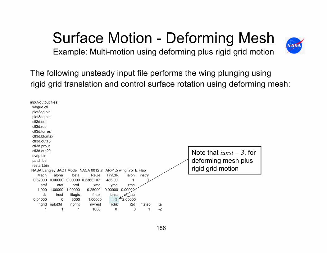
186
Surface Motion - Deforming MeshExample: Multi-motion using deforming plus rigid grid motion
The following unsteady input file performs the wing plunging using rigid grid translation and control surface rotation using deforming mesh:
input/output files: wbgrid.cflplot3dg.bin plot3dq.bin cfl3d.out cfl3d.rescfl3d.turres cfl3d.blomaxcfl3d.out15 cfl3d.prout cfl3d.out20 ovrlp.binpatch.binrestart.bin
NASA Langley BACT Model: NACA 0012 af, AR=1.5 wing,.75TE FlapMach alpha beta ReUe Tinf,dR ialph ihstry
0.82000 0.00000 0.00000 0.236E+07 486.00 1 0sref cref bref xmc ymc zmc
1.000 1.00000 1.00000 0.25000 0.00000 0.00000dt irest iflagts fmax iunst cfl_tau
0.04000 0 3000 1.00000 3 2.00000ngrid nplot3d nprint nwrest ichk i2d ntstep ita
1 1 1 1000 0 0 1 -2
Note that iunst = 3, for deforming mesh plusrigid grid motion

187
Surface Motion - Deforming MeshExample: Multi-motion using deforming plus rigid grid motion
ncg iem iadvance iforce ivisc(i) ivisc(j) ivisc(k)2 0 0 1 5 5 5
idim jdim kdim73 345 73
ilamlo ilamhi jlamlo jlamhi klamlo klamhi0 0 0 0 0 0
inewg igridc is js ks ie je ke0 0 0 0 0 0 0 0
idiag(i) idiag(j) idiag(k) iflim(i) iflim(j) iflim(k)1 1 1 3 3 3
ifds(i) fds(j) ifds(k) rkap0(i) rkap0(j) rkap0(k)1 1 1 0.3333 0.3333 0.3333
grid nbci0 nbcidim nbcj0 nbcjdim nbck0 nbckdim iovrlp1 1 1 1 1 5 1 0
i0: grid segment bctype jsta jend ksta kend ndata1 1 1001 1 345 1 73 0
idim: grid segment bctype jsta jend ksta kend ndata1 1 1002 1 345 1 73 0
j0: grid segment bctype ista iend ksta kend ndata1 1 1003 1 73 1 73 0
jdim: grid segment bctype ista end ksta kend ndata1 1 1003 1 73 1 73 0
k0: grid segment bctype ista iend jsta jend ndata1 1 0 1 49 1 33 01 2 2004 1 49 33 313 2
tw/tinf cq0.00000 0.00000
1 3 0 1 49 313 345 01 4 0 49 73 1 173 01 5 0 49 73 173 345 0
kdim: grid segment bctype ista iend jsta jend ndata 1 1 1003 1 73 1 345 0
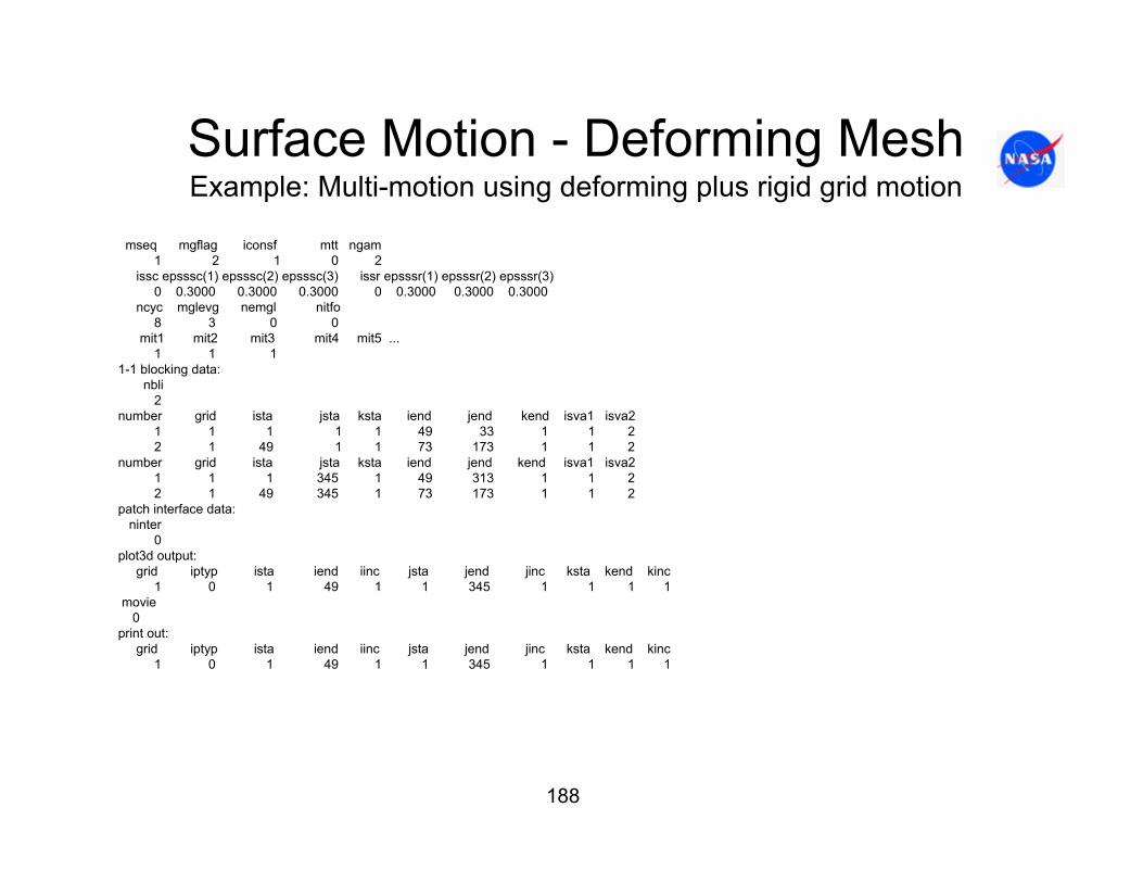
188
Surface Motion - Deforming MeshExample: Multi-motion using deforming plus rigid grid motion
mseq mgflag iconsf mtt ngam1 2 1 0 2
issc epsssc(1) epsssc(2) epsssc(3) issr epsssr(1) epsssr(2) epsssr(3)0 0.3000 0.3000 0.3000 0 0.3000 0.3000 0.3000
ncyc mglevg nemgl nitfo8 3 0 0
mit1 mit2 mit3 mit4 mit5 ...1 1 1
1-1 blocking data:nbli
2number grid ista jsta ksta iend jend kend isva1 isva2
1 1 1 1 1 49 33 1 1 22 1 49 1 1 73 173 1 1 2
number grid ista jsta ksta iend jend kend isva1 isva21 1 1 345 1 49 313 1 1 2 2 1 49 345 1 73 173 1 1 2
patch interface data:ninter
0plot3d output:
grid iptyp ista iend iinc jsta jend jinc ksta kend kinc1 0 1 49 1 1 345 1 1 1 1
movie0
print out:grid iptyp ista iend iinc jsta jend jinc ksta kend kinc
1 0 1 49 1 1 345 1 1 1 1

189
Surface Motion - Deforming MeshExample: Multi-motion using deforming plus rigid grid motion
Control Surfaces:ncs0
Grid ista iend jsta jend ksta kend iwall inormmoving grid data - rigid translation (forced motion):
ntrans1
lref1.0grid itrans rfreq utrans vtrans wtrans
1 2 0.10 0.00 0.00 5.00 grid dxmax dymax dzmax
1 10. 10. 10.moving grid data - rigid rotation (forced motion):
nrotat0
lrefgrid irotat rfreq omegax omegay omegaz xorig yorig zoriggrid dthxmx dthymx dthzmxMoving grid data – deforming surface (forced motion):ndefrm
2lref1.0
Grid idefrm rfreq u/omegax v/omegay w/omegaz xorig yorig zorig1 2 0.05 0.00 10.00 0.00 0.75 0.00 0.001 2 0.05 0.00 10.00 0.00 0.75 0.00 0.00
Grid icsi icsf jcsi jcsf kcsi kcsf1 25 37 33 65 1 1 1 25 37 281 313 1 1
Rigid grid motioninput
Surface motioninput

190
Surface Motion - Deforming MeshExample: Multi-motion using deforming plus rigid grid motion
Moving grid data – aeroelastic surface (aeroelastic motion):naesrf
0Iaesrf ngrid grefl uinf qinf nmodes iskyhookFreq gmass damp x0(2n-1) xo(2n) gf0(2n)
Moddfl amp freq t0Grid iaei iaef jaei jaef kaei kaef
Moving grid data – data for field/multiblock mesh movementnskip isktyp beta1 alpha1 beta2 alpha2 nsprgit
0 -2 1.0 1.1 1.0 0.005 0Control point index inputMoving grid data – multi-motion couplingncoupl
1Slave master xorig yorig zorig
1 1 0.75 0.00 0.00
Note: CFL3D does not allow initiating new kinds of motion upon restarts. Therefore if an initial deforming mesh computation is performed to reach an equilibrium before initiating a combined rigid and moving (deforming) control surface computation, the option iunst = 3 must be used from the start (that is after an initial steady state computation with dt < 0), with control surface motion set to zero.
Multi-motion coupling data included
Aeroelastic header linesincluded
Deforming mesh input

191
Aeroelastic AnalysisOverview
• CFL3D has the capability to perform both static and dynamic aeroelastic analysis. In this analysis the fluid and structure interact through a time marching simulation (e.g. flutter analysis, etc…)
• All aeroelastic and modal analyses are performed by running the code in unsteady mode
• CFL3D performs aeroelastic analysis for a linear structure modally and a linear and nonlinear structure when loosely coupled with either NASTRANor ABAQUS finite element analyses.
• For modal analysis, the equations of structural dynamics must be decoupled modally– Eigenvalue analysis is required prior to running CFD to obtain frequencies, generalized
masses and mode shapes. – A preprocessing step projecting the mode shapes onto the CFD surface grids is required.– The code reads the modal data projected onto the CFD surfaces in the file ‘aesurf.dat’. This
file must be contained in the directory in which the executable resides.• CFL3D also has the capability to perform unsteady deforming body analysis using
mode shapes. In this mode the user specifies modal motion (e.g. control surface rotation, wing plunge oscillation, etc…) in the aeroelastic input section

192
Aeroelastic AnalysisExample of an aeroelastic model
Consider the Benchmark Active Controls Technology (BACT) aeroelastic model shown. The model has pitch and plunge aeroelastic degrees of freedom. The model parameters are:
MT = 5.966 slugsSα = 0.01420 slug-ftIα = 2.8017 slug-ft2Kh = 2659 lb/ftKa = 2897 lb-ft/rad
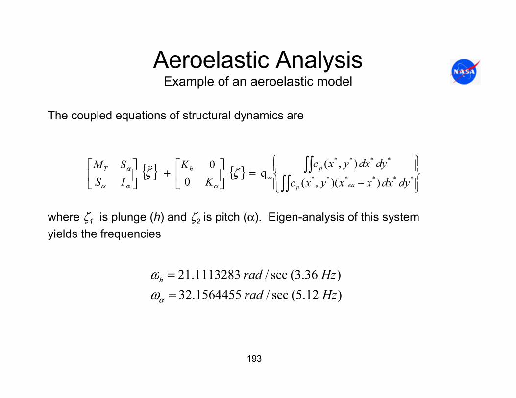
193
Aeroelastic AnalysisExample of an aeroelastic model
The coupled equations of structural dynamics are
where ζ1 is plunge (h) and ζ2 is pitch (α). Eigen-analysis of this system yields the frequencies
{ } { }⎪⎭
⎪⎬⎫
⎪⎩
⎪⎨⎧
−=⎥
⎦
⎤⎢⎣
⎡+⎥
⎦
⎤⎢⎣
⎡
∫∫∫∫
∞ ******
****
))(,(
),(q
00
dydxxxyxc
dydxyxcK
KISSM
eap
phT ζζααα
α &&
)12.5(sec/1564455.32)36.3(sec/1113283.21
HzradHzradh
==
αωω

194
Aeroelastic AnalysisExample of an aeroelastic model
Using the eigenvectors
the generalized masses are obtained
5974345042.0001571926.0
0024991919.0409404775.0
2221
1211⎥⎦
⎤⎢⎣
⎡−
=⎥⎦
⎤⎢⎣
⎡=
ϕϕϕϕ
φ
000000000.1000000000.1
2
1
==
mm

195
Aeroelastic AnalysisExample of an aeroelastic model
… and the decoupled equations of structural dynamics
where
Carrying through the multiplication on the right-hand side, we have
{ } { }⎪⎭
⎪⎬⎫
⎪⎩
⎪⎨⎧
−=⎥
⎦
⎤⎢⎣
⎡+⎥
⎦
⎤⎢⎣
⎡
∫∫∫∫
∞ ******
****T1-
22
21
))(,(
),(qM
00
1001
dydxxxyxc
dydxyxcqq
eap
pφω
ω&&
⎥⎦
⎤⎢⎣
⎡=
2
1
00
mm
M
{ } { }⎪⎭
⎪⎬⎫
⎪⎩
⎪⎨⎧
−+
−+=⎥
⎦
⎤⎢⎣
⎡+⎥
⎦
⎤⎢⎣
⎡
∫∫∫∫
∞ ****2212
**
****2111
**1-
22
21
)}(){,(
)}({),(qM
00
1001
dydxxxyxc
dydxxxyxcqq
eap
eap
ϕϕϕϕ
ωω
&&
qφζ = φφω
ωα⎥⎦
⎤⎢⎣
⎡=⎥
⎦
⎤⎢⎣
⎡K
Km
m hT
00
00
222
211
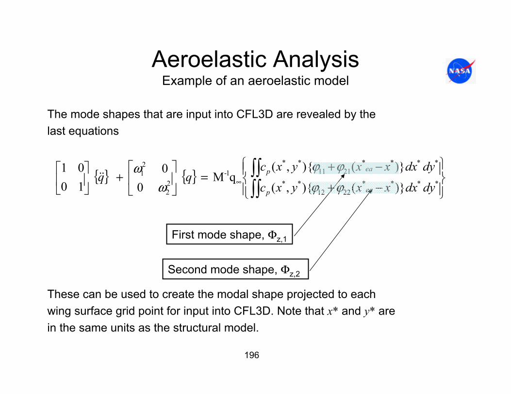
196
Aeroelastic AnalysisExample of an aeroelastic model
The mode shapes that are input into CFL3D are revealed by the last equations
These can be used to create the modal shape projected to each wing surface grid point for input into CFL3D. Note that x* and y* are in the same units as the structural model.
{ } { }⎪⎭
⎪⎬⎫
⎪⎩
⎪⎨⎧
−+
−+=⎥
⎦
⎤⎢⎣
⎡+⎥
⎦
⎤⎢⎣
⎡
∫∫∫∫
∞ ****2212
**
****2111
**1-
22
21
)}(){,(
)}({),(qM
00
1001
dydxxxyxc
dydxxxyxcqq
eap
eap
ϕϕϕϕ
ωω
&&
First mode shape, Φz,1
Second mode shape, Φz,2
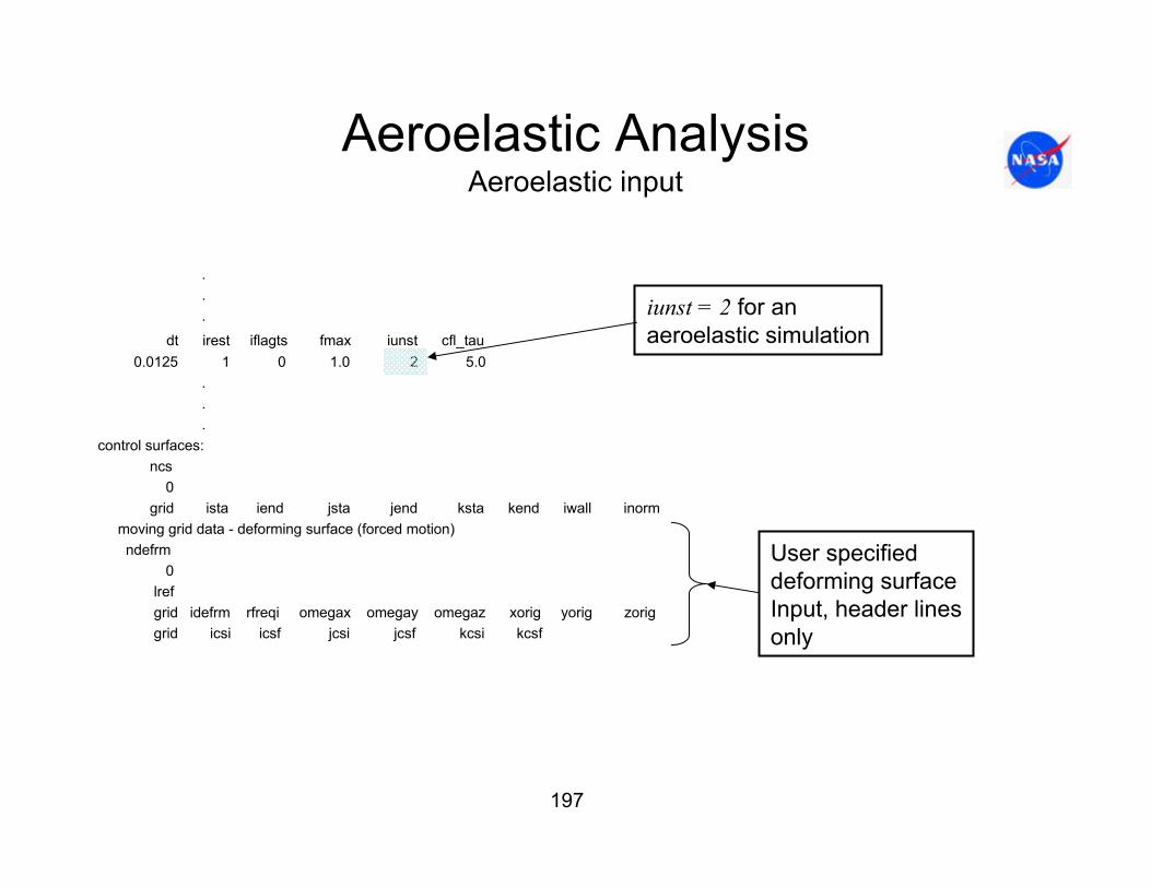
197
Aeroelastic AnalysisAeroelastic input
.
.
.
dt irest iflagts fmax iunst cfl_tau0.0125 1 0 1.0 2 5.0
.
.
.control surfaces:
ncs0
grid ista iend jsta jend ksta kend iwall inormmoving grid data - deforming surface (forced motion)ndefrm
0lrefgrid idefrm rfreqi omegax omegay omegaz xorig yorig zoriggrid icsi icsf jcsi jcsf kcsi kcsf
iunst = 2 for an aeroelastic simulation
User specifieddeforming surfaceInput, header linesonly
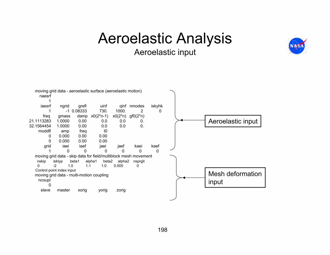
198
Aeroelastic AnalysisAeroelastic input
moving grid data - aeroelastic surface (aeroelastic motion)naesrf
1 iaesrf ngrid grefl uinf qinf nmodes iskyhk
1 -1 0.08333 730. 1000. 2 0 freq gmass damp x0(2*n-1) x0(2*n) gf0(2*n)
21.1113283 1.0000 0.00 0.0 0.0 0.32.1564454 1.0000 0.00 0.0 0.0 0.
moddfl amp freq t00 0.000 0.00 0.000 0.000 0.00 0.00
grid iaei iaef jaei jaef kaei kaef1 0 0 0 0 0 0
moving grid data - skip data for field/multiblock mesh movementnskip isktyp beta1 alpha1 beta2 alpha2 nsprgit0 -2 1.0 1.1 1.0 0.005 0
Control point index inputmoving grid data - multi-motion coupling
ncoupl0
slave master xorig yorig zorig
Aeroelastic input
Mesh deformationinput

199
Aeroelastic AnalysisAeroelastic input
Focusing on the aeroelastic input section:
moving grid data - aeroelastic surface (aeroelastic motion)naesrf
1 iaesrf ngrid grefl uinf qinf nmodes iskyhk
1 -1 0.08333 730. 1000. 2 0 freq gmass damp x0(2*n-1) x0(2*n) gf0(2*n)
21.1113283 1.0000 0.00 0.0 0.0 0.32.1564454 1.0000 0.00 0.0 0.0 0.
moddfl amp freq t00 0.000 0.00 0.000 0.000 0.00 0.00
grid iaei iaef jaei jaef kaei kaef1 0 0 0 0 0 0
iaesrf - Identifier of the aeroelastic surface for which data is being suppliedngrid - Number of surface segments that make up this aeroelastic surfacenmodes - Number of modes to be modeled in CFL3Diskyhk - Not currently used, any value will serve as a placeholderuinf - Free-stream velocity, in the same units as the equations of structural dynamicsqinf - Dynamic pressure, in the same units as the equations of structural dynamicsgrefl - Conversion from CFD grid units to structural equation units.
Number of aeroelasticsurfaces
naesrf lines
nmodes lines
one line only whenngrid = -1 (Currently this Is the only option)

200
Aeroelastic AnalysisAeroelastic input
Regarding the input parameter grefl, consider the equations of structural dynamics for thepitch/plunge example:
The actual equations solved in CFL3D are:
{ } { }⎪⎭
⎪⎬⎫
⎪⎩
⎪⎨⎧
Φ
Φ=⎥
⎦
⎤⎢⎣
⎡+⎥
⎦
⎤⎢⎣
⎡
∫∫∫∫
∞ **2,
**
**1,
**1-
22
21
),(
),(qM
00
1001
dydxyxc
dydxyxcqq
zp
zp
ωω
&&
{ } { }⎪⎭
⎪⎬⎫
⎪⎩
⎪⎨⎧
Φ
Φ=⎥
⎦
⎤⎢⎣
⎡+⎥
⎦
⎤⎢⎣
⎡
∫∫∫∫
∞ dydxyxc
dydxyxcqq
zp
zp
1,
1,1-222
21
),(
),(qMgrefl
00
1001
ωω
&&
Lengths in CFDgrid units
Lengths in structuralmodel units
CFDAE SSgrefl /=By definition:

201
Aeroelastic AnalysisAeroelastic input
In the present example the structural equations are in units of feet, while the CFD grid is in units of inches. Note that the aspect ratios of the original and rescaled model must be identical. Conversion for the present example can be obtained from
This is the grefl parameter that would be entered in the aeroelastic input section.
unitgridftSSgrefl CFDAE /08333.0144
1/ ≈==

202
Aeroelastic AnalysisModal form of the equations
Consider the decoupled equations of structural dynamics for N (or nmodes in theinput) modes
where q is the modal variable vector and Q is the generalized force vector, each oflength N. ω1 ,…, ωN are the natural frequencies of each structural mode in radians, and m1 ,…, mN are the generalized masses.
{ } { } { }
{ }Qm000000m
00
0000
200
00002
10000001
1-N
1-1
2
2111
⎥⎥⎥
⎦
⎤
⎢⎢⎢
⎣
⎡
=
⎥⎥⎥
⎦
⎤
⎢⎢⎢
⎣
⎡
+⎥⎥⎥
⎦
⎤
⎢⎢⎢
⎣
⎡+
⎥⎥⎥
⎦
⎤
⎢⎢⎢
⎣
⎡
O
O&O&&O qqq
NNN ω
ω
ζω
ζω

203
Aeroelastic AnalysisModal form of the equations
CFL3D input definitions as they relate to the modal equations of structural dynamics are as follows:
Units for frequency is radians/time (usually time scale is secondsfor the structural dynamics equations).
initNinit
initNinit
initNinit
N
N
N
QNgfQgf
qNxqx
qNxqxNdampingdampingNfreqfreq
mNgmassmgmass
==
==
=−=======
)*2(0,,)2(0
)*2(0,,)2(0
)1*2(0,,)1(0)(,,)1()(,,)1()(,,)1(
1
1
1
1
1
1
L
&L&
L
L
L
L
ζζωω

204
• x0(2*n-1) is the initial generalized displacement of the mode; will override the value in the restart file (if restarting) when x0(2*n-1) is nonzero. Otherwise, it will not override the restart value. This allows the mode to be perturbed for excitation of aeroelastic dynamic response after a static aeroelastic starting solution has been performed.
• x0(2*n) is the initial generalized velocity of the mode; will override the value in the restart file (if restarting) when x0(2*n) is nonzero. Otherwise, it will not override the restart value. This allows the mode to be perturbed for excitation of aeroelastic dynamic response after a static aeroelastic starting solution has been performed.
• gf0(2*n) is the generalized force offset to include for the mode. This value is included in CFL3D computation of generalized force in the following way for mode n = 1 to nmodes:
Aeroelastic AnalysisAeroelastic input
{ } )*2(02 ngfsdcgreflqQ npn −⋅Φ= ∫∫∞rr
Value from input

205
Aeroelastic AnalysisMethod of integrating the fluid/structure coupling based
on the state transition matrix solution
n -1 n n + 1
F lu id
S tru c tu re
( )1211 3~ −+ −Θ+Θ= nn
inn QQxx
( )nni
nn QQxx +Θ+Θ= ++ 1211
1~ +nx
The structural dynamic equations are written in state space form and solvedusing the state transition matrix solution and a predictor/corrector scheme. The fluid/structure cycling is shown below:
1+nQ
Predictor step:
After the predictor step, the structure surface is moved using the predicted modal solution , the flow field is converged to the solution at time step n+1, and the new generalized force is computed.
Corrector step:

206
The parameter is the state transition matrix. The parameter is the discrete integration of the state input, and is the state vector containing the generalized aerodynamic force at time step n. The solution and generalizedforce state vectors are
The value is the intermediate state solution used to update the mesh.
This method uses a second order backward differencing of the fluid/structure coupling. Combined with second order backward differenced fluid dynamics solver and the second order backward differencing of the mesh time metrics, the overall scheme is second order accurate. For the original method see: Edwards, J. W., Bennett, R. M., Whitlow Jr., W., Seidel, D. A.,“Time-Marching Transonic Flutter Solutions Including Angle-of-Attack Effects,” Journal of Aircraft, 20 (1983), pg. 899-906.
Aeroelastic AnalysisMethod of integration and fluid/structure coupling
Θ iΘnQ
⎪⎪⎪
⎭
⎪⎪⎪
⎬
⎫
⎪⎪⎪
⎩
⎪⎪⎪
⎨
⎧
=
⎪⎪⎪
⎭
⎪⎪⎪
⎬
⎫
⎪⎪⎪
⎩
⎪⎪⎪
⎨
⎧
=
NN
N
Q
x0
0
,11
1
M
&
M
&
x~

207
Aeroelastic AnalysisModal surface input
• Currently CFL3D assumes that the aeroelastic surface comprises all boundary segments with the boundary condition types 1005, 1006, 2004, 2014 or 2016.
• Note that the boundary condition 1001 is not considered an aeroelastic surface. Therefore, if a symmetry plane is required to deform with a pitching wing, it must be treated as an inviscid wall boundary (1005 or 1006)
• The modal input file aesurf.dat must have modal data for a given surface point in free field ascii format (no commas) with Φx,n, Φy,n, Φz,n modal deflections at each surface point for each mode n.

208
Aeroelastic AnalysisFormat of the modal surface input
The following ordering is required:
j = 1 surface:Φx,n(i,j,k) Φy,n(i,j,k) Φz,n(i,j,k) ,k = ksta to kend , i = ista to iend , repeat nseg times
j = jdim surface:Φx,n(i,j,k) Φy,n(i,j,k) Φz,n(i,j,k) ,k = ksta to kend , i = ista to iend , repeat nseg times
k = 1 surface:Φx,n(i,j,k) Φy,n(i,j,k) Φz,n(i,j,k) , j = jsta to jend , i = ista to iend , repeat nseg times
k = kdim surface:Φx,n(i,j,k) Φy,n(i,j,k) Φz,n(i,j,k) , j = jsta to jend , i = ista to iend , repeat nseg times
i = 1 surface:Φx,n(i,j,k) Φy,n(i,j,k) Φz,n(i,j,k) , j = jsta to jend , k = ksta to kend , repeat nseg times
i = idim surface:Φx,n(i,j,k) Φy,n(i,j,k) Φz,n(i,j,k) , j = jsta to jend, k = ksta to kend , repeat nseg times,
Repeat all of the above input for n = 1 to nmodes, repeat ngrid times, repeat naesrf times.
Segment limits defined inboundary condition input

209
Aeroelastic AnalysisFormat of the modal surface input
• The ordering of the aeroelastic surface points must correspond to the order of the points in the CFD grid file read by CFL3D.
• Aeroelastic segments must be input in the same block order as the grid file, and segments must be input in order of ascending indices.
• When creating a multi zonal grid using the utility ‘splitter’, be aware that the final ordering will generally not correspond to the ordering of the unsplit grid. Ordering of the split grid zones can be found in the ‘splitter.out’ file, from which can be found the required order of the surface grid points for the ‘aesurf.dat’ file.
Example: Consider a block face that has dimensions kdim = 49, idim = 49 with several aeroelastic segments. If segment 1 has indices k = 33 to 49, i = 13 to 33, and segment 2 has indices k = 1 to 33, i = 1 to 33, then segment 2 must be input first.

210
Aeroelastic AnalysisAeroelastic output
• Aeroelastic time history output is in the file ‘genforce.dat’. • This file is generated if iunst = 2 and aeroelastic surfaces
are defined in the input file (naesrf≠0).• After header information, modal response data for each
mode is written sequentially. • Unlike output data in the ‘cfl3d.subit_res’ file, a complete
time history of this data for the entire simulation is retained and written/read to/from restart files and subsequently output to the ‘genforce.dat’ file.

211
Aeroelastic AnalysisAeroelastic output
Consider the example output contained in the ‘genforce.dat’ file:
NASA Langley BACT Model: NACA 0012 af, AR=1.5 wing,.75TE FlapMach= 0.7700E+00, alpha= 0.0000E+00, ReUe= 0.3860E+07Number of aeroelastic surfaces = 1Data for aeroelastic surface 1mode number 1
it time xs(2*n-1) xs(2*n) gforcn(2*n)1 0.3125000E-01 0.0000000E+00 0.0000000E+00 -0.3471162E-052 0.6250000E-01 0.0000000E+00 0.0000000E+00 -0.3214494E-053 0.9375000E-01 0.0000000E+00 0.0000000E+00 -0.2996337E-054 0.1250000E+00 0.0000000E+00 0.0000000E+00 -0.2789857E-05
mode number 2it time xs(2*n-1) xs(2*n) gforcn(2*n)1 0.3125000E-01 0.2980232E-09 0.3442899E-09 0.6291896E-052 0.6250000E-01 0.3089730E-09 0.3565678E-09 0.6644112E-053 0.9375000E-01 0.3203131E-09 0.3692693E-09 0.6907312E-054 0.1250000E+00 0.3320569E-09 0.3824084E-09 0.7143990E-05
Time - Non-dimensional time (CFL3D non-dimensionalization)xs(2*n-1) - Modal or generalized variable outputxs(2*n) - Modal velocity outputgforcn(2*n) - Modal or generalized force output
Title line from the input file
Data from the input file
Mode 1 time historyfrom starting run
Mode 2 time historyfrom starting run

212
Aeroelastic AnalysisStrategy for aeroelastic computations
The following strategies may be used for performing static or dynamic aeroelastic simulations
• Static aeroelastic computations can be performed by:– Start either from scratch (irest = 0), or restart, after a steady state computation (in
which dt < 0, iunst = 0). Starting from scratch is not recommended.– Set iunst = 2 , dt > 0 and damp = .99999… and perform the computation in a time
marching manner to convergence.
• Flutter onset computations can be performed by:– Converging a static solution as outlined above.– Setting damp to the correct value for the elastic system being modeled.– Setting an initial perturbation x0(2*n) or x0(2*n-1) in the desired mode.*
* If a restart in the middle of a flutter computation is performed, the initial perturbation values from the previous run must be reset to zero at the restart of the new run.
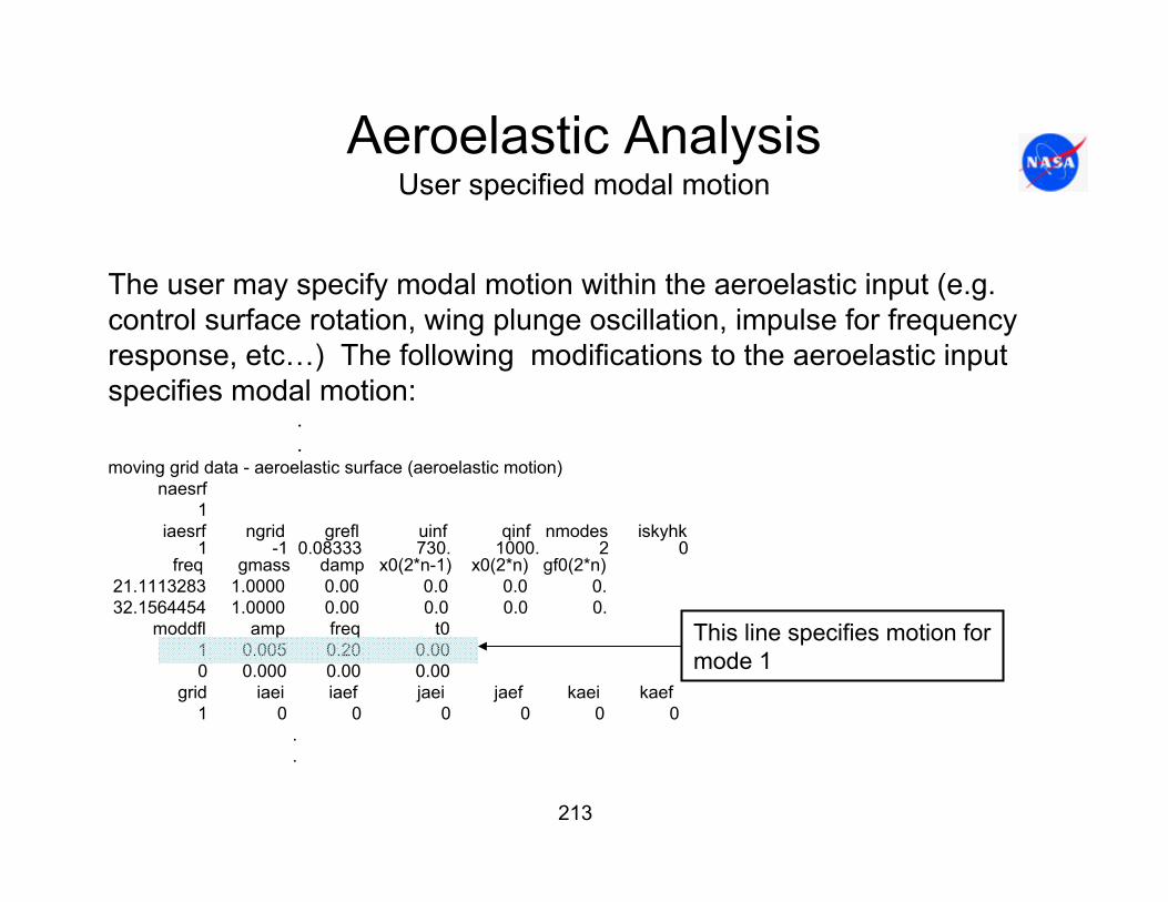
213
Aeroelastic AnalysisUser specified modal motion
The user may specify modal motion within the aeroelastic input (e.g. control surface rotation, wing plunge oscillation, impulse for frequency response, etc…) The following modifications to the aeroelastic input specifies modal motion:
.
.moving grid data - aeroelastic surface (aeroelastic motion)
naesrf1
iaesrf ngrid grefl uinf qinf nmodes iskyhk1 -1 0.08333 730. 1000. 2 0
freq gmass damp x0(2*n-1) x0(2*n) gf0(2*n)21.1113283 1.0000 0.00 0.0 0.0 0.32.1564454 1.0000 0.00 0.0 0.0 0.
moddfl amp freq t01 0.005 0.20 0.000 0.000 0.00 0.00
grid iaei iaef jaei jaef kaei kaef1 0 0 0 0 0 0
.
.
This line specifies motion formode 1

214
Aeroelastic AnalysisUser specified modal motion
moddfltype of time-varying modal perturbation desired: < 0, mode displacement and velocity set to zero= 0, no perturbation (solution via the dynamic modal equations) = 1, harmonic (sinusoidal) perturbation = 2, Gaussian pulse = 3, step pulse
A (amp)amplitude of modal perturbation.
ωr (freq)reduced frequency of modal perturbation if moddfl = 1 half-width of Gaussian pulse if moddfl = 2 use any value as a placeholder for moddfl = 0
t0 (t0)time about which Gaussian pulse is centered if moddfl = 2 time of the step pulse if moddfl = 3 use any value as a placeholder for moddfl = 0

215
Aeroelastic AnalysisUser specified modal motion
For harmonic perturbation the modal displacement and velocities for mode nare computed in the following way:
where A = amp, ωr = freq in radians per dimensional time, and t* is dimensional time,
(uinf) is in the aeroelastic input section and is from the main aerodynamic input section. t is CFL3D non-dimensional time.
For a Gaussian pulse the displacement and velocity for mode n are computed with
)cos(,)sin( ** tAkqtAq rrnrn ωω == &
[ ] [ ]2/)2log(
2,2
0*2
0*
r
ttCn
ttCn
Cwhere
CAeqAeq
ω=
−== −−−− &
∞∞∞∞ == MUaagrefltt /,/*
∞U ∞M

216
Aeroelastic AnalysisUser specified modal motion
For step pulse the modal displacement and velocities for mode nare computed in the following way:
0,2
,22
0,02
0
*
0*
*
*
0*
*
0
0
*
0*
==∆+>
∆==∆+<<∆−
==∆−<
nn
nn
nn
qAqthenttttif
tAqAqthentttttif
qqthenttttif
&
&
&

217
For this example:
Recommend sizing time step so that there are an absolute minimum of 25 time steps within the half life of the pulse (∆t = kr/25). In this case we would have ∆t = 0.004.
0 0.25 0.5 0.75 10
0.1
0.2
0.3
0.4
0.5
0.6
0.7
0.8
0.9
1
q
t
Aeroelastic AnalysisExample: Gaussian modal pulse and time step sizing
Time to reach half height
20
/)2log(
/5.0,1.0,0.1
r
r
C
agrefltkA
ω=
=== ∞
greflat /0 ∞
1.0/ == ∞agreflk rr ω
∞∞∞∞ == MUaagrefltt /,/*
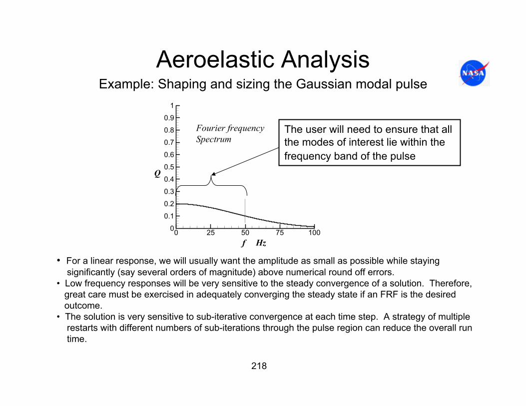
218
Aeroelastic AnalysisExample: Shaping and sizing the Gaussian modal pulse
0 25 50 75 1000
0.1
0.2
0.3
0.4
0.5
0.6
0.7
0.8
0.9
1
Q
f Hz
The user will need to ensure that all the modes of interest lie within the frequency band of the pulse
Fourier frequencySpectrum
• For a linear response, we will usually want the amplitude as small as possible while staying significantly (say several orders of magnitude) above numerical round off errors.
• Low frequency responses will be very sensitive to the steady convergence of a solution. Therefore, great care must be exercised in adequately converging the steady state if an FRF is the desired outcome.
• The solution is very sensitive to sub-iterative convergence at each time step. A strategy of multiplerestarts with different numbers of sub-iterations through the pulse region can reduce the overall run time.
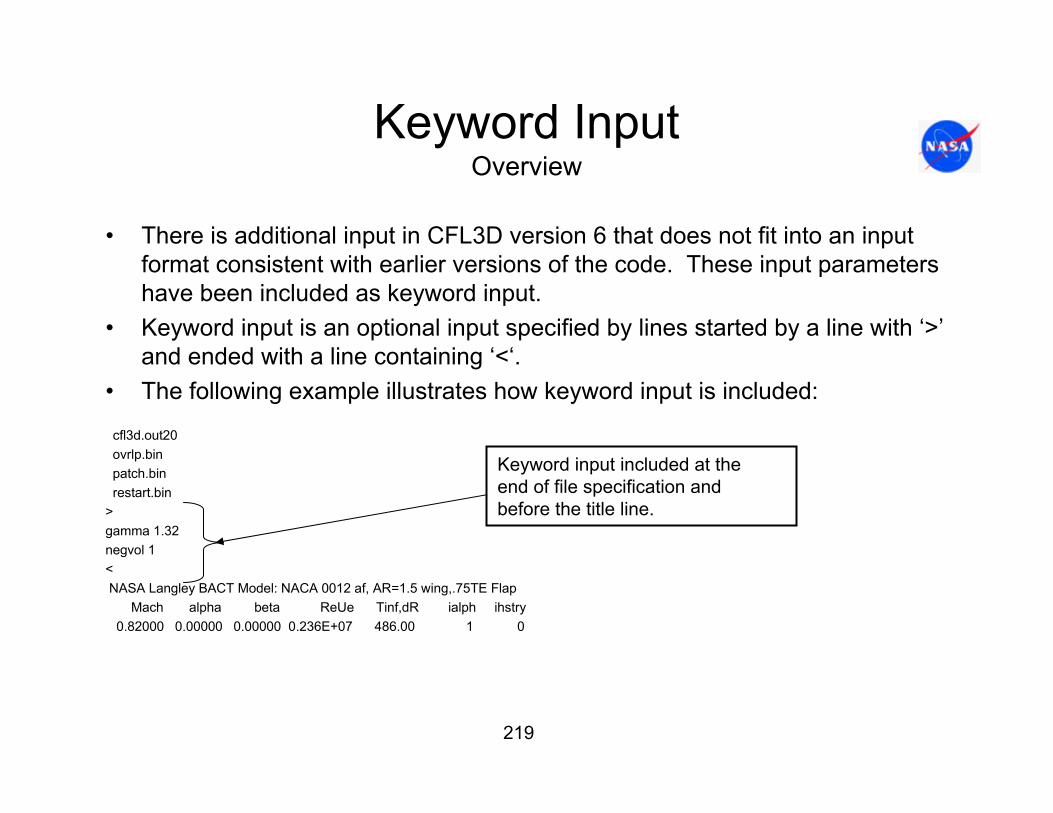
219
Keyword InputOverview
• There is additional input in CFL3D version 6 that does not fit into an input format consistent with earlier versions of the code. These input parameters have been included as keyword input.
• Keyword input is an optional input specified by lines started by a line with ‘>’and ended with a line containing ‘<‘.
• The following example illustrates how keyword input is included:
cfl3d.out20 ovrlp.binpatch.binrestart.bin
>gamma 1.32negvol 1<NASA Langley BACT Model: NACA 0012 af, AR=1.5 wing,.75TE Flap
Mach alpha beta ReUe Tinf,dR ialph ihstry0.82000 0.00000 0.00000 0.236E+07 486.00 1 0
Keyword input included at theend of file specification and before the title line.

220
Keyword InputValid Keywords
Name Description Default Value
cbar Ref. temp. for Sutherland Law 198.6
gamma Ratio of specific heats 1.4
pr Prandtl number 0.72
prt Turbulent Prandtl number 0.90
Physical Properties
Name Description Default Value
atol Tolerance for detecting singular lines 10-7
epsa_r Eigenvalue limiter (entropy fix for high Mach flows) 0.0
Limiters

221
Keyword InputValid Keywords
Name Description Default Value
avn Factor multiplying uref for preconditioning 1.0
cprec Relative amount of preconditioning 0.0
uref Limiting velocity for preconditioning xmach
Preconditioning
Name Description Default Value
cltarg Target Cl 99999.
dalim Limit of alpha change (deg) per update 0.2
icycupdt Number of cycles between alpha updates (if > 0; if < 0, alpha is never updated)
1
rlxalph Relaxation factor used to update angle of attack 1.0
Specified CL

222
Keyword InputValid Keywords
Name Description Default Value
cflturb Cfl no. for turbl eqns. = cflturb x abs(dt) If cflturb > 0 0(model dependent default)
edvislim Limiter for eddy viscosity in 2-equationturb models; eddy viscosity limited to edvislim times the
laminar viscosity
100000.
ibeta8kzeta flag (0/1) to set beta8 term when using k-enstrophyturbulence model (ivisc=15); 0 = use beta8=0.0 (helps avoid
numerical problems); 1 = use beta8=2.3 (available afterV6.3)
0
ides flag (0/1) to perform DES with turbulence model (1) or not (0)
0
cdes constant associated with DES 0.65
ieasmcc2d flag (0/1) to turn on 2-D curvature correction when using EASM models (ivisc=8,9,11,12,13,14) (1) or not (0)
(available after V6.3)
0
isarc2d flag (0/1) to turn on 2-D curvature correction when using SA model (ivisc=5) (1) or not (0) (available after V6.3)
0
Turbulence models

223
Keyword InputValid Keywords
Name Description Default Value
sarccr3 value of cr3 parameter in SARC model (available after V6.3) 0.6
ikoprod flag: 0=use approximate (vorticity-based) turb production term (-2*mut*WijWji) for turb models 6, 7, 10, or 15; 1=use strain-rate based term (2*mut*SijSij); 2=use full production
term (ivisc=15 only) (available after V6.3)
0(vorticity-based
production)
isstdenom flag (0/1): 0=use vorticity term in denominator of eddyviscosity in SST model (#7); 1=use strain term
(available after V6.3)
0(vorticity term)
itaturb flag (0/1) to control time accuracy of turb. model; 0 for 1st order in time regardless of parameter "ita" for the mean flow;
1 for same order as set by ita
1(turb. Time accuracy
same as mean flow, set via ita)
iturbord flag controls whether turbulence model advection terms are 1st or 2nd order upwind on RHS (1=1st, 2=2nd) (note: LHS
uses 1st order in both cases) (available after V6.3)
1(1st order)
Turbulence models
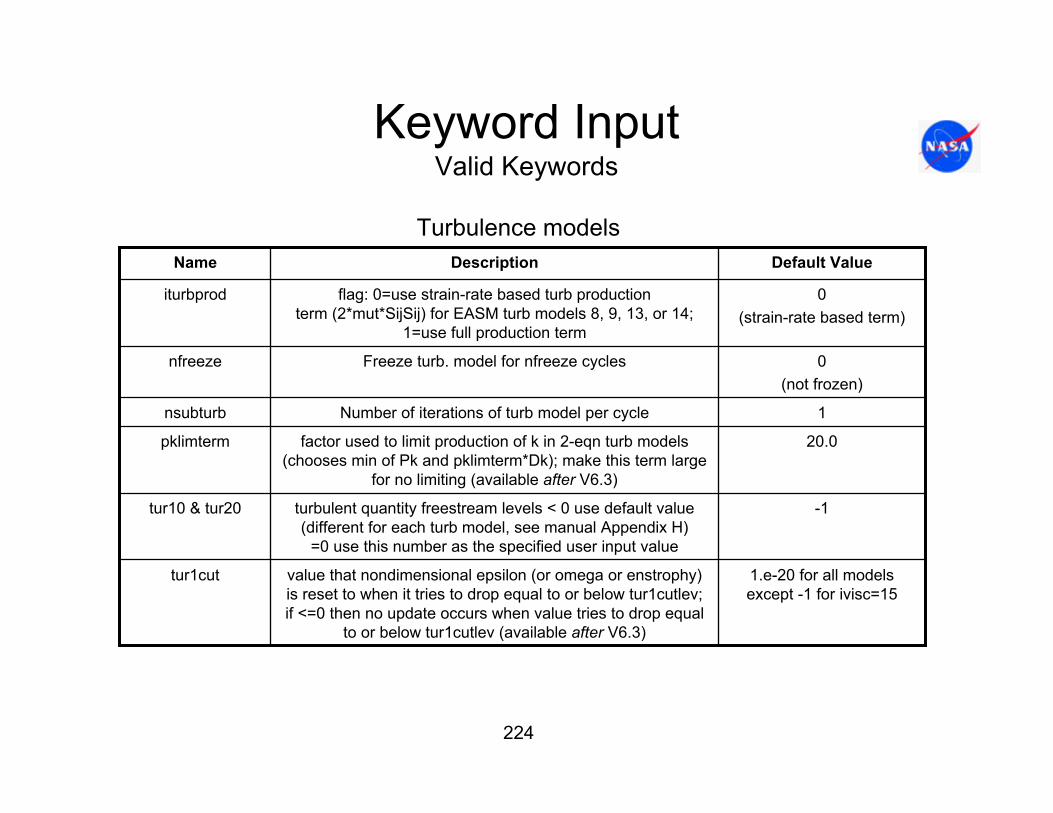
224
Keyword InputValid Keywords
Name Description Default Value
iturbprod flag: 0=use strain-rate based turb productionterm (2*mut*SijSij) for EASM turb models 8, 9, 13, or 14;
1=use full production term
0(strain-rate based term)
nfreeze Freeze turb. model for nfreeze cycles 0(not frozen)
nsubturb Number of iterations of turb model per cycle 1
pklimterm factor used to limit production of k in 2-eqn turb models (chooses min of Pk and pklimterm*Dk); make this term large
for no limiting (available after V6.3)
20.0
tur10 & tur20 turbulent quantity freestream levels < 0 use default value (different for each turb model, see manual Appendix H)
=0 use this number as the specified user input value
-1
tur1cut value that nondimensional epsilon (or omega or enstrophy) is reset to when it tries to drop equal to or below tur1cutlev; if <=0 then no update occurs when value tries to drop equal
to or below tur1cutlev (available after V6.3)
1.e-20 for all models except -1 for ivisc=15
Turbulence models

225
Keyword InputValid Keywords
Name Description Default Value
tur2cut value that nondimensional k is reset to when it tries to drop equal to or below tur2cutlev; if <=0 then no update occurs
when value tries to drop equal to or below tur2cutlev(available after V6.3)
1.e-20
tur1cutlev & tur2cutlev
lower levels of nondimensional epsilon (or omega or enstrophy)
and k which, when reached, cause the turb quantities to be reset to tur1cut or tur2cut (available after V6.3)
0
Turbulence models

226
Keyword InputValid Keywords
Name Description Default Value
idef_ss flag (0/1) to deform volume grid to surface in file newsurf.p3d
0(don’t deform)
meshdef flag (0/1) to bypass flow solution while still computing grid operations such as metrics and volumes; 0 = normal
operation; 1 = bypass flow solution (available after V6.3)
0
negvol flag (0/1) to enable/disable stop if neg. volumes/bad metrics are detected
0(stop for negative volumes)
Deformation/grid motion
Name Description Default Value
ibin flag (0/1) for formatted/unformatted output plot3d files
1 (unformatted)
iblnk flag (0/1) for un-iblanked/iblanked output plot3d files
1 (iblanked)
Input/output control

227
Keyword InputValid Keywords
Name Description Default Value
iblnkfr flag (0/1) for un-iblanked/iblanked fringe points in plot3d files (overset grids only)
1(iblanked)
icgns flag (0/1) to not use/use CGNS files* 0 (don’t use CGNS files)
ip3dgrad flag (0/1) for solution/derivative data output to plot3d q file (complex code only)
0(solution to q file)
irghost flag to read ghost-cell data from restart file (1) or not (0); V5 restart files and Beta V6 restart files do not contain ghost-cell data; newer V6 restart files
do
1(read ghost-cell data)
iwghost flag to write ghost-cell data to restart file (1) or not (0); V5 restart files and Beta V6 restart files do not contain ghost-cell data; newer V6 restart files do
1(write ghost-cell data)
Input/output control

228
Keyword InputValid Keywords
Name Description Default Value
itime2read flag (0/1) to skip/read 2nd order (in time)turbulence terms and dt in restart file: need to skip if using an older time-accurate-with-2nd-order-time
restart file
1(read 2nd order time
turbulence terms and dt)
iteravg flag to store iteration-averaged conserved variables in PLOT3D files: 0 = no averaging or
storage 1 = start averaging now2 = continue averaging from previous run
0
Input/output control
Name Description Default Value
memadd additional memory (in words) added to work array(in case sizer underestimates)
0(no addition to work)
memaddi additional memory (in words) added to iwork array(in case sizer underestimates)
0 (no addition to iwork)
Memory management

229
Keyword InputValid Keywords
Name Description Default Value
noninflag flag (0/1) to indicate whether to use inertial (0) or noninertial (1) reference frame for governing
equations; noninertial frames allow for steady state solutions if the rotation rate is constant
0(inertial reference frame)
xcentrot rotation center x-coordinate for non-inertial reference frame (also used for roll-angle input)
0.0
ycentrot rotation center y-coordinate for non-inertial reference frame (also used for roll-angle input)
0.0
xrotate rotation rate about x-axis for non-inertial reference frame (non-dimensionalized the same way as
omegax for rotating grids - see manual)
0.0
yrotate rotation rate about y-axis for non-inertial reference frame (non-dimensionalized the same way as
omegay for rotating grids - see manual)
0.0
zcentrot rotation center z-coordinate for non-inertial reference frame (also used for roll-angle input)
0.0
zrotate rotation rate about z-axis for non-inertial reference frame (non-dimensionalized the same way as
omegaz for rotating grids - see manual)
0.0
Reference frame

230
Keyword InputValid Keywords
Name Description Default Value
xrotrate_img complex perturbation to rotation rate about x-axis for non-inertial reference frame, for computing rate
derivatives
0.0
yrotrate_img complex perturbation to rotation rate about y-axis for non-inertial reference frame, for computing rate
derivatives
0.0
zrotrate_img complex perturbation to rotation rate about z-axis for non-inertial reference frame, for computing rate
derivatives
0.0
Reference frame
Name Description Default Value
alpha_img Imaginary perturbation to alpha 0.0
beta_img Imaginary perturbation to beta 0.0
geom_img Imaginary perturbation to grid 0.0
Other

231
Keyword InputValid Keywords
Name Description Default Value
reue_img Imaginary perturbation to unit Re 0.0
surf_img Imaginary perturbation to surface grid 0.0
ifullns flag (0/1) to specify inclusion of cross-derivative terms; 0 = thin-layer N-S; 1 = full N-S (available
after V6.3)
0
ivolint flag (0/1) to use approximate/exact one-to-oneboundary volumes (0 emulates V5.0)
1 (exact volumes)
tinf_img Imaginary perturbation to Tinf 0.0
xmach_img Imaginary perturbation to Mach no. 0.0
iaxi2plane flag for use with particular axisymmetric cases (for which i2d=0 and idim=2); if iaxi2plane = 1, the time step based on CFL number is modified so it does not depend on the i-direction metrics (available
after V6.3)
0(no mods to time step)
roll_angle x-axis roll angle (deg) "+" is clockwise viewed from "- x" (left roll to pilot) (grid is rotated to this angle)
0.0
Other

232
Block Splitting and MPIOverview
• Message Passing Interface (MPI) protocol is used for parallelization of CFL3D
• MPI parallelizes by parceling out grid blocks to different processors• For MPI to be useful, at least two or more blocks and at least three
processors will be required.• Often grids will arrive as multiple block grids. However, there are several
reasons that additional block splitting will be required:– If the original mesh is not split into a sufficient number of blocks to efficiently use
the processors available.– If the blocks are of disparate sizes, so that load balancing will be difficult.

233
Block Splitting and MPIOverview
• Note, however, that there is a limit on the number of blocks for a given overall grid size for which efficient parallelization can take place.
– Problem of growing communications between processors compared toprocessing per block (communication time).
– Because CFL3D treats block boundaries explicitly, splitting into an ever increasing number of blocks amounts to making the code explicit. An increasingnumber of blocks means that an increasing number of sub-iterations will be required.
• The following illustrates the increasing communications with decreasing block sizes….

234
Block Splitting and MPIProblem of the humming bird versus the elephant
0 25 50 75 100
0.1
0.2
0.3
0.4
0.5
0.6
0.7
0.8
0.9
1
R
idim
Consider the ratio of number of surface points to the total number of grid points as grid size diminishes. These results are based on a grid having equal idim, jdim, kdim dimensions.
volumeareasurfaceR =
At an average dimension of 10x10x10, boundary data takes a third ofthe total memory. (Whichis not a problem for MPI, but…communication becomesa growing percentage ofthe computation time.)
235
Block Splitting and MPIOverview
With the issues clearly in mind, there are times when splitting is useful…
• The tool ‘splitter’ is available with CFL3D for use in splitting blocks. • It is created by performing the following command in the ‘build’ directory:
make splitter
• The executable will be in the directory ‘~/cfl3dv6/build/split/seq/’.• An example input can be found in the CFL3D version 6 web page.

236
Block Splitting and MPIExample: Splitting a single C-H grid
Lets consider again the BACT wing we have looked at previously. This grid has i,j,k dimensions 73 (spanwise) x 345 (streamwise) x 73 (normal to wing).
Suppose a 32 processor PC clusteris available for this problem. It wouldbe useful to split this block into at least24 blocks. However consideration must also be given to how many times each dimension can be split and still retain the proper dimensionsto perform multi-grid computations.

237
Block Splitting and MPIExample: Splitting a single C-H grid
An acceptable block split can be obtained by requiring M, the number of split blocks, in the following computation
be an integer. D is the overall dimension of the un-split grid, and d is the proposed dimension of the split grid. For the current example, the j-dimension can be split with blocks having dimension of 9, 87 or 173.
11
−−=
dDM
211731345,4
1871345,43
191345 =
−−==
−−==
−−= MMM

238
Block Splitting and MPIExample: Splitting a single C-H grid
Note that block dimensions of 87 or 173 will allow only 3 levels of multigrid, a dimension of 9 allows 4. We will chose a dimension of 87.
Similar computations for the idim = 73 and kdim = 73 lead us to chose 6 blocks in those directions with dimension of 13. This will result in a total of 144 blocks. This number of blocks will allow us to use 4, 24, 48 or 144 processors efficiently.
These computations result in 3 splits in the j-direction, 5 splits in the i-direction and 5 splits in the k-direction for a total of 13 splits. The input that performs these splits is shown in the next slide.
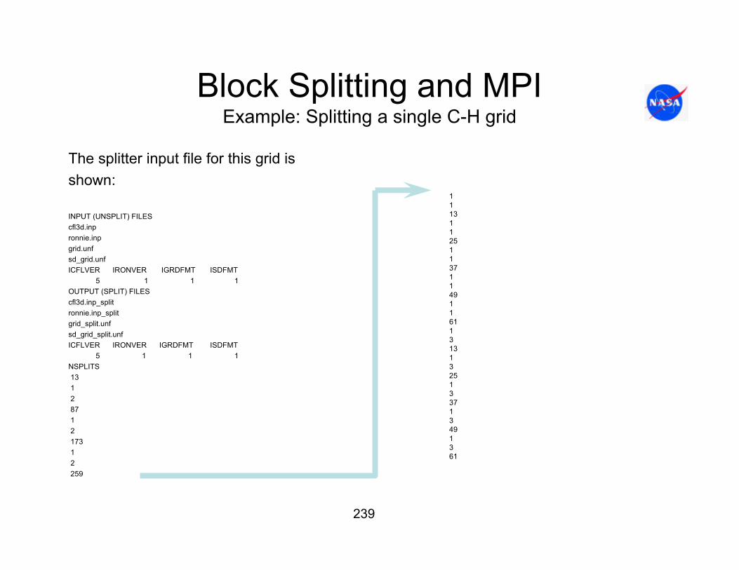
239
Block Splitting and MPIExample: Splitting a single C-H grid
The splitter input file for this grid is shown:
INPUT (UNSPLIT) FILES cfl3d.inp ronnie.inpgrid.unfsd_grid.unfICFLVER IRONVER IGRDFMT ISDFMT
5 1 1 1 OUTPUT (SPLIT) FILES cfl3d.inp_split ronnie.inp_splitgrid_split.unfsd_grid_split.unfICFLVER IRONVER IGRDFMT ISDFMT
5 1 1 1 NSPLITS 1312 87 12 173 12259
1113112511371149116113131325133713491361
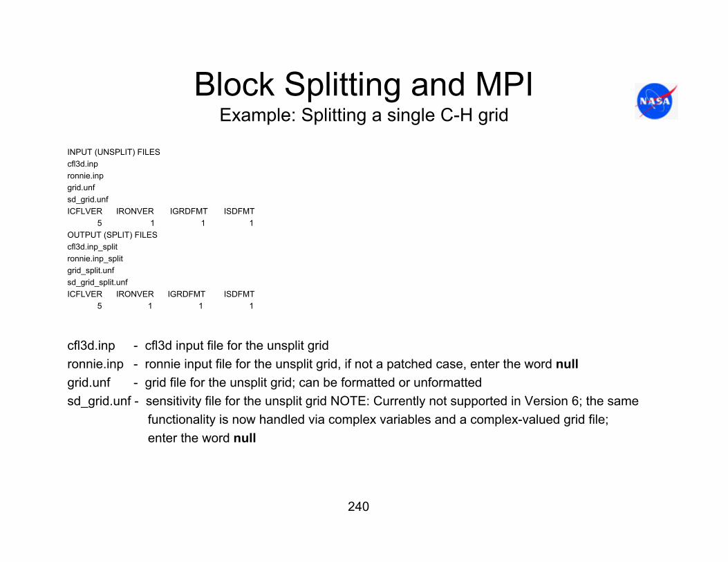
240
Block Splitting and MPIExample: Splitting a single C-H grid
INPUT (UNSPLIT) FILES cfl3d.inp ronnie.inpgrid.unfsd_grid.unfICFLVER IRONVER IGRDFMT ISDFMT
5 1 1 1 OUTPUT (SPLIT) FILES cfl3d.inp_split ronnie.inp_splitgrid_split.unfsd_grid_split.unfICFLVER IRONVER IGRDFMT ISDFMT
5 1 1 1
cfl3d.inp - cfl3d input file for the unsplit grid ronnie.inp - ronnie input file for the unsplit grid, if not a patched case, enter the word null grid.unf - grid file for the unsplit grid; can be formatted or unformatted sd_grid.unf - sensitivity file for the unsplit grid NOTE: Currently not supported in Version 6; the same
functionality is now handled via complex variables and a complex-valued grid file; enter the word null
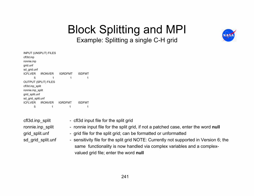
241
Block Splitting and MPIExample: Splitting a single C-H grid
INPUT (UNSPLIT) FILES cfl3d.inp ronnie.inpgrid.unfsd_grid.unfICFLVER IRONVER IGRDFMT ISDFMT
5 1 1 1 OUTPUT (SPLIT) FILES cfl3d.inp_split ronnie.inp_splitgrid_split.unfsd_grid_split.unfICFLVER IRONVER IGRDFMT ISDFMT
5 1 1 1
cfl3d.inp_split - cfl3d input file for the split grid ronnie.inp_split - ronnie input file for the split grid, if not a patched case, enter the word nullgrid_split.unf - grid file for the split grid; can be formatted or unformatted sd_grid_split.unf - sensitivity file for the split grid NOTE: Currently not supported in Version 6; the
same functionality is now handled via complex variables and a complex-valued grid file; enter the word null

242
Block Splitting and MPIExample: Splitting a single C-H grid
INPUT (UNSPLIT) FILES cfl3d.inp ronnie.inpgrid.unfsd_grid.unfICFLVER IRONVER IGRDFMT ISDFMT
5 1 1 1 OUTPUT (SPLIT) FILES cfl3d.inp_split ronnie.inp_splitgrid_split.unfsd_grid_split.unfICFLVER IRONVER IGRDFMT ISDFMT
5 1 1 1
icflver= 4 the cfl3d input file is a version 4.1 type = -4 the cfl3d input file is a version 4.1hp type = 5 the cfl3d input file is a version 5/6 type
ironver= 0 ronnie input file is the old style, with all "from" blocks listed on one line = 1 ronnie input file is the new style, with each "from" block having it's own line NOTE: a value for ironver must always be entered, even if the case does not involve patched grids.
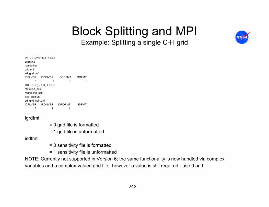
243
Block Splitting and MPIExample: Splitting a single C-H grid
INPUT (UNSPLIT) FILES cfl3d.inp ronnie.inpgrid.unfsd_grid.unfICFLVER IRONVER IGRDFMT ISDFMT
5 1 1 1 OUTPUT (SPLIT) FILES cfl3d.inp_split ronnie.inp_splitgrid_split.unfsd_grid_split.unfICFLVER IRONVER IGRDFMT ISDFMT
5 1 1 1
igrdfmt= 0 grid file is formatted = 1 grid file is unformatted
isdfmt= 0 sensitivity file is formatted = 1 sensitivity file is unformatted
NOTE: Currently not supported in Version 6; the same functionality is now handled via complex variables and a complex-valued grid file; however a value is still required - use 0 or 1

244
Block Splitting and MPIExample: Splitting a single C-H grid
.
.NSPLITS 1312 87 12 173 12259
.
.
nsplits - number of grid splits to perform (can be 0 in order to convert grid from formatted to unformatted or vice versa). Following the value of nsplits, nsplits triplets of integers must appear, one integer of the triplet per line….
nsplits

245
Block Splitting and MPIExample: Splitting a single C-H grid
..
NSPLITS 1312 87 12 173 12259
.
.
iblk - block number of the block to be split. NOTE: iblk always refers to the original, unsplitblock number
ldir= 1 split in the i-direction = 2 split in the j-direction = 3 split in the k-direction
index - split the block in the ldir direction at this value of the index
iblk
ldir
index
Same triplet repeated 13 times

246
Block Splitting and MPIExample: Splitter output
* * * * * * * * * * * * * * * * * * * * * * * * * * * * * * * * * * * * * * * * * * * * * * * * * * * ** * SPLITTER - CFL3D BLOCK AND INPUT FILE SPLITTER * ** * * ** * VERSION 6.X : Computational Fluids Lab, Mail Stop 128, * ** * NASA Langley Research Center, Hampton, VA * ** * Release Date: MMM DD, YYYY. * ** * * *
* * * * * * * * * * * * * * * * * * * * * * * * * * * * * * * * * * * * * * * * * * * * * * * * * * * * * * * * * * * * * * * * * * * * * * * * * * * * * * * * * * * * * * * * * * * * * * * *
memory allocation: 431.046108 Mbytes, double precision
input (unsplit) filescfl3d.inpnullwbgrid.cflnull
icflver ironver igrdfmt isdfmt5 1 1 1
output (split) filescfl3d.inp_splitnullwbgrid_split.cflnull
icflver ironver igrdfmt isdfmt5 1 1 1

247
Block Splitting and MPIExample: Splitter output
converting unsplit cfl3d input file to tlns3d map file
checking dimensions...
reading grid...grid: wbgrid.cfl
block # 1: il= 73, jl= 345, kl= 73
number of splits = 13split block coord index
1 1 J 872 1 J 1733 1 J 2594 1 I 135 1 I 256 1 I 377 1 I 498 1 I 619 1 K 13
10 1 K 2511 1 K 3712 1 K 4913 1 K 61
new block old block i0 i1 j0 j1 k0 k11 1 1 13 1 87 61 732 1 1 13 87 173 61 733 1 1 13 173 259 61 734 1 1 13 259 345 61 735 1 13 25 259 345 61 736 1 13 25 173 259 61 737 1 13 25 87 173 61 738 1 13 25 1 87 61 739 1 25 37 1 87 61 7310 1 25 37 87 173 61 7311 1 25 37 173 259 61 7312 1 25 37 259 345 61 7313 1 37 49 259 345 61 7314 1 37 49 173 259 61 7315 1 37 49 87 173 61 7316 1 37 49 1 87 61 7317 1 49 61 1 87 61 7318 1 49 61 87 173 61 7319 1 49 61 173 259 61 7320 1 49 61 259 345 61 7321 1 61 73 259 345 61 7322 1 61 73 173 259 61 7323 1 61 73 87 173 61 7324 1 61 73 1 87 61 7325 1 61 73 1 87 49 6126 1 61 73 87 173 49 6127 1 61 73 173 259 49 6128 1 61 73 259 345 49 61

248
Block Splitting and MPIExample: Splitter output
29 1 49 61 259 345 49 6130 1 49 61 173 259 49 6131 1 49 61 87 173 49 6132 1 49 61 1 87 49 6133 1 37 49 1 87 49 6134 1 37 49 87 173 49 6135 1 37 49 173 259 49 6136 1 37 49 259 345 49 6137 1 25 37 259 345 49 6138 1 25 37 173 259 49 6139 1 25 37 87 173 49 6140 1 25 37 1 87 49 6141 1 13 25 1 87 49 6142 1 13 25 87 173 49 6143 1 13 25 173 259 49 6144 1 13 25 259 345 49 6145 1 1 13 259 345 49 6146 1 1 13 173 259 49 6147 1 1 13 87 173 49 6148 1 1 13 1 87 49 61
.
.
.
.
.
.121 1 61 73 1 87 1 13122 1 61 73 87 173 1 13123 1 61 73 173 259 1 13124 1 61 73 259 345 1 13125 1 49 61 259 345 1 13126 1 49 61 173 259 1 13127 1 49 61 87 173 1 13128 1 49 61 1 87 1 13129 1 37 49 1 87 1 13130 1 37 49 87 173 1 13131 1 37 49 173 259 1 13132 1 37 49 259 345 1 13133 1 25 37 259 345 1 13134 1 25 37 173 259 1 13135 1 25 37 87 173 1 13136 1 25 37 1 87 1 13137 1 13 25 1 87 1 13138 1 13 25 87 173 1 13139 1 13 25 173 259 1 13140 1 13 25 259 345 1 13141 1 1 13 259 345 1 13142 1 1 13 173 259 1 13143 1 1 13 87 173 1 13144 1 1 13 1 87 1 13
split-grid basic dimensions are multigridable to ncg = 1
Input points: 1838505Ouput points: 2117232

249
Block Splitting and MPI
Notes regarding use:
• IF A LIMITER IS DESIRED, USE IFLIM=4. This will allow for consistent results with block splitting; iflim=3 is not recommended - iflim=4 is basically a correct implementation of iflim=3 for multiple blocks, and should now be viewed as the recommended limiter for any case that needs one.
• Also, for exact consistency between split and unsplit grids, version 5 emulation (i.e. "Install -v5) should not be used. Version 5 (and earlier versions) made anapproximation for cell volumes at 1-1 block interfaces that has been eliminated in version 6 in favor of the exact treatment.
• The input file part of the splitter works by first converting the unsplit CFL3D input file to a TLNS3D map file, splitting the TLNS3D map file, then converting the split TLNS3D map file back to a CFL3D input file.
250
Block Splitting and MPI
Notes (...continued):
• Caveats: The conversions from the CFL3D input file to a TLNS3D map file are not perfect! The user is urged check the resulting split CFL3D input (and patch) files.
– A useful check before actually splitting the files is to run this splitter with the number of splittings = 0, and the output grid file as null. Running splitter in this way will cause to code to go through the translations, but the "split" files will have the same numbers of blocks, and the "split" grid will not be output.
– A "diff" or "gdiff" will point to translation-induced differences that should be easier to sort out than when coupled with true splitting. Note that the 2-step process almost always results in a *reordering* of some boundary condition segments.

251
Running CFL3D in MPI mode
• MPI requires one processor for overhead. For example if a 32 processor cluster is employed, and there are 28 blocks to be computed on 28 processors, then the command line will read:
mpirun –np 29 cfl3d_mpi < cfl3d.inp &
• You may want to verify the correct procedure for running mpi code on your platform (e.g. some mpp's use -n instead of -np)
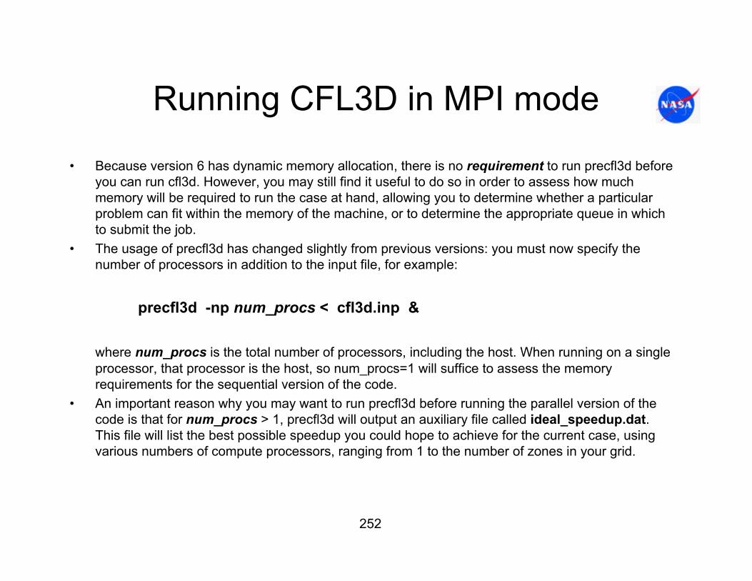
252
Running CFL3D in MPI mode
• Because version 6 has dynamic memory allocation, there is no requirement to run precfl3d before you can run cfl3d. However, you may still find it useful to do so in order to assess how much memory will be required to run the case at hand, allowing you to determine whether a particular problem can fit within the memory of the machine, or to determine the appropriate queue in which to submit the job.
• The usage of precfl3d has changed slightly from previous versions: you must now specify the number of processors in addition to the input file, for example:
precfl3d -np num_procs < cfl3d.inp &
where num_procs is the total number of processors, including the host. When running on a single processor, that processor is the host, so num_procs=1 will suffice to assess the memory requirements for the sequential version of the code.
• An important reason why you may want to run precfl3d before running the parallel version of the code is that for num_procs > 1, precfl3d will output an auxiliary file called ideal_speedup.dat. This file will list the best possible speedup you could hope to achieve for the current case, using various numbers of compute processors, ranging from 1 to the number of zones in your grid.
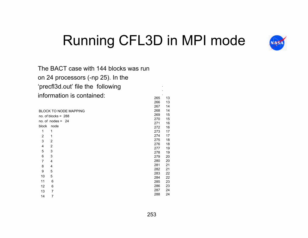
253
Running CFL3D in MPI mode
The BACT case with 144 blocks was run on 24 processors (-np 25). In the ‘precfl3d.out’ file the following information is contained:
BLOCK TO NODE MAPPINGno. of blocks = 288no. of nodes = 24block node
1 12 13 24 25 36 37 48 49 5
10 511 612 613 714 7
.
.
.265 13266 13267 14268 14269 15270 15271 16272 16273 17274 17275 18276 18277 19278 19279 20280 20281 21282 21283 22284 22285 23286 23287 24288 24

254
Running CFL3D in MPI mode..
**************************************************************
SUMMARY OF STORAGE REQUIREMENTS - W + WK ARRAYS
sequential version:
permanent array w requires 131825665 (words)temporary array wk requires 2681342 (words)temporary array iwk requires 187820 (words)
parallel version, per node:
permanent array w requires 5506908 (words)temporary array wk requires 1500235 (words)temporary array iwk requires 187820 (words)
>>> Estimate for mwork (sequential) = 134507007 <<<
>>> Estimate for mworki (sequential) = 187820 <<<
>>> Estimate for mwork (per node, parallel) = 7007143 <<<
>>> Estimate for mworki (per node, parallel) = 187820 <<<
>>> Parallel code sized for 24 nodes, min. (+host) <<<
**************************************************************
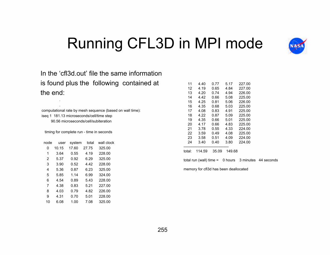
255
Running CFL3D in MPI mode
In the ‘cfl3d.out’ file the same information is found plus the following contained at the end:
.
.computational rate by mesh sequence (based on wall time):iseq 1 181.13 microseconds/cell/time step
90.56 microseconds/cell/subiteration
timing for complete run - time in seconds
node user system total wall clock0 10.15 17.60 27.75 325.00 1 3.64 0.55 4.19 228.002 5.37 0.92 6.29 325.003 3.90 0.52 4.42 228.00 4 5.36 0.87 6.23 325.00 5 5.85 1.14 6.99 324.00 6 4.54 0.89 5.43 228.00 7 4.38 0.83 5.21 227.008 4.03 0.79 4.82 226.009 4.31 0.70 5.01 228.00
10 6.08 1.00 7.08 325.00
11 4.40 0.77 5.17 227.0012 4.19 0.65 4.84 227.0013 4.20 0.74 4.94 226.00 14 4.42 0.66 5.08 225.00 15 4.25 0.81 5.06 226.00 16 4.35 0.68 5.03 225.00 17 4.08 0.83 4.91 225.00 18 4.22 0.87 5.09 225.0019 4.35 0.66 5.01 225.0020 4.17 0.66 4.83 225.00 21 3.78 0.55 4.33 224.0022 3.59 0.49 4.08 225.0023 3.58 0.51 4.09 224.0024 3.40 0.40 3.80 224.00
------------------------------------total: 114.59 35.09 149.68
total run (wall) time = 0 hours 3 minutes 44 seconds
memory for cfl3d has been deallocated

256
Flow Field VisualizationPlot3D output
CFL3D is capable of creating Plot3D files of the grid and flow field. Specification of the region of the flow field for output is found in the following input lines:
.
.dt irest iflagts fmax iunst cfl_tau
-2.0 0 0 1.0 0 5.0ngrid nplot3d nprint nwrest ichk i2d ntstep ita
1 1 1 1000 0 1 1 -2ncg iem iadvance iforce ivisc(i) ivisc(j) ivisc(k)
2 0 0 1 0 0 5..
plot3d output:grid iptyp ista iend iinc jsta jend jinc ksta kend kinc
1 0 1 1 1 1 999 1 1 999 1movie
0
nplot3d specifies the numberof blocks to output
Input nplot3dlines
If nplot3d < 0, then the Plot3D files are automatically set to include all solid Surfaces (no field points) for 3D cases or all field points for 2D cases

257
Flow Field VisualizationPlot3D output
..
plot3d output:grid iptyp ista iend iinc jsta jend jinc ksta kend kinc
1 0 1 1 1 1 999 1 1 999 1movie
0
Grid - Designated grid number to be outputiptyp = 0 - grid point type – grid file and Q file output
= 1 - cell center type – grid file and Q file output= 2 - cell center type - grid file and turbulence file output (ivisc > 1 only)> 2 - cell center type – grid file and function file output (iptype = 3 – minimum distance to
nearest viscous wall or directed distance (ivisc > 1 only), iptype = 4 – eddy viscosity (ivisc > 1 only)
ista, jsta, ksta - starting indices in the i,j,k directionsiend,jend,kend - ending indices in the i,j,k directions (note that if these values are set higher than
idim, jdim,kdim, the code will reset them to the block dimensions)iinc,jinc,kinc - increment in the i,j,k directions
Note: Setting ista = iend = iinc = 0, etc… is a short hand way of specifying the entire range.

258
Flow Field VisualizationMovie output
.
.plot3d output:
grid iptyp ista iend iinc jsta jend jinc ksta kend kinc1 0 1 1 1 1 999 1 1 999 1
movie10
Note that one gird file and one solutions file are generated.
Movie = 0 no output of intermediate solutions (if nplot3d > 0), then a single solution is written at the end of the run.Movie > 0 output of additional solutions every movie iterations (time steps)Movie < 0 output of the initial flow field at the beginning of the run and output of additional solutions every movie
iterations (time steps)
Caution: Use with care. Plot3D file will get very large very quickly.
The tool ‘moovmaker’ will read the plot3D solution and grid file and create a movie for a 2D flow field in which the 3rd
dimension will be time. The grid output by ‘moovmaker will be called ‘g.bin’ and the solution file will be called ‘q.bin’. Creating these files will allow animating the 3rd dimension (time) to produce a movie of the flow field.
Flag to append Plot3D solution outputevery 10 time steps
259
Useful CFL3D Tools
• Get_FD.F– This program reads two CFL3D restart files and calculate finite differences of force and
moment coefficients; it is used to validate complex-variable approach for determining solution derivatives.
• INGRID_to_p3d.F – This program converts PEGSUS 4.x INGRID file to a PLOT3D file that can be used in
CFL3D. Note that the INGRID file must correspond to grid points rather than "augmented" cell centers.
• XINTOUT_to_ovrlp.F– This program converts the XINTOUT overset grid interpolation file from PEGSUS to the
ovrlp.bin file used by CFL3D. • cfl3d_to_pegbc.F
– This program creates a peg.bc.raw file for use with PEGSUS 5.x. • cgns_to_cfl3dinput.F
– This program reads a CGNS file and creates a PLOT3D-type grid as well as a best-guess for a CFL3D input file.

260
Useful CFL3D Tools
• everyother_xyz.F– This program reads a grid and creates an every-other-point grid. This can be useful in
combination with the program v6inpdoubhalf.F, in order to reduce the required CFL3D run-time memory when you are only running on a coarser-level grid (and not taking it up to the finer level(s).
• grid_perturb.F– This program generates a real-valued grid (PLOT3D multiblock form) by reading in a real-
valued grid (PLOT3D multiblock form) and a corresponding real-valued matrix of grid-sensitivity derivatives (PLOT3D multiblock function file form, with 3*ndv variables for the x,y,zcomponents of the ndv design variables). The code Get_FD.F may be used with the two restart files to determine d(Cl)/d(DV), d(Cd)/d(DV), etc.
• grid_perturb_cmplx.F– This program generates a complex-valued grid (PLOT3D multiblock form) by reading in a
real-valued grid (PLOT3D multiblock form) and a corresponding real-valued matrix of grid-sensitivity derivatives (PLOT3D multiblock function file form, with 3*ndv variables for the x,y,zcomponents of the ndv design variables). The output grid may be read into the complexversion of CFL3D (cfl3dcmplx_mpi or cfl3dcmplx_seq) to determine the solution derivatives with respect to the chosen design variable.

261
Useful CFL3D Tools
• initialize_field.F– This program creates a restart.bin restart file in which you can specify specific initial
conditions, region by region. This can be useful when "freestream everywhere" is not a desirable initial condition.
• moovmaker.F– This program reads the PLOT3D files output by CFL3D when the MOVIE parameter is used
for 2-D datasets (or 3-D datasets surface-only), and creates new PLOT3D files with time as the third (k) direction.
• p3d_to_INGRID.F – This program converts either PLOT3D or CFL3D type grids into either INGRID type grids that
can be used with PEGSUS 4.x, or PLOT3D type grids that can be used with PEGSUS 5.x. The converted grids can contain either the grid points as given in the input grids, or "augmented" cell centers of the input grids.
• p3d_to_cfl3drst.F – This program reads PLOT3D files and creates an approximate restart.bin restart file. This
can be useful if: (1) you are given a PLOT3D Q-file from another code, and you wish to use it as a basis for starting CFL3D, or (2) you have lost the CFL3D restart file, but you still have the PLOT3D Q-file.

262
Useful CFL3D Tools
• plot3dg_to_cgns.F – This program reads a PLOT3D grid file and a CFL3D input file and creates a CGNS file (with
grid, BC, and 1-to-1 connectivity information in it). • v6_restart_mod.F
– This program reads a restart.bin restart file and manipulates it. It can switch between unformatted and formatted (which is useful if you need to transfer the restart file to a machine of different architecture). It can also write out the restart file either the same size, half the size, or double the size. Going to half size is useful if one wishes to restart from a fine grid solution and run on a coarser level. User can choose to coarsen/refine only particular index directions, if desired. The program cannot both coarsen and refine different directions simultaneously.
• v6inpdoubhalf.F – This program reads a CFL3D input file and creates a new input file appropriate for a grid of
either half or double the size. This can be useful in combination with the program everyother_xyz.F when running on coarser grid levels, and you wish to reduce the run-time memory required.

263
References
Edwards, J. W., Bennett, R. M., Whitlow Jr., W., Seidel, D. A., “Time-Marching Transonic Flutter Solutions Including Angle-of-Attack Effects,”Journal of Aircraft, 20 (1983), pp. 899-906.
Lee-Rausch, E. M., Batina, J. T., “Wing flutter boundary prediction using unsteady Euler method,” Journal of Aircraft, 32 (1995), pp. 416-422.
Krist, S. L., “CFL3D User’s Manual (Version 5.0),” NASA/TM-1998-208444, June 1998.
Bartels, R. E., “Mesh Strategies for Accurate Computation of Unsteady Spoiler and Aeroelastic Problems,” Journal of Aircraft, 37 (2000), pp. 521-525.
CFL3D version 6.0 web site: http://cfl3d.larc.nasa.gov/Cfl3dv6/cfl3dv6.html.Bartels, R. E., “Finite Macro-Element Mesh Deformation in a Structured
Multi-Block Navier-Stokes Code,” NASA/TM-2005-213789, July 2005.

264
Summary
• CFL3D is a general purpose production-level CFD code for fluid dynamics, with many capabilities and options.
• This tutorial has summarized many of the newest features of the code, and also has explained in detail how to set up and run it for general cases.
• Particular focus has been given to CFL3D’s upgraded deforming mesh and aeroelastic analysis capabilities.

REPORT DOCUMENTATION PAGE Form ApprovedOMB No. 0704-0188
2. REPORT TYPE Technical Memorandum
4. TITLE AND SUBTITLE
CFL3D Version 6.4—General Usage and Aeroelastic Analysis5a. CONTRACT NUMBER
6. AUTHOR(S)
Bartels, Robert E.; Rumsey, Christopher L; and Biedron, Robert T.
7. PERFORMING ORGANIZATION NAME(S) AND ADDRESS(ES)
NASA Langley Research CenterHampton, VA 23681-2199
9. SPONSORING/MONITORING AGENCY NAME(S) AND ADDRESS(ES)
National Aeronautics and Space AdministrationWashington, DC 20546-0001
8. PERFORMING ORGANIZATION REPORT NUMBER
L-19247
10. SPONSOR/MONITOR'S ACRONYM(S)
NASA
13. SUPPLEMENTARY NOTESAn electronic version can be found at http://ntrs.nasa.gov
12. DISTRIBUTION/AVAILABILITY STATEMENTUnclassified - UnlimitedSubject Category 01Availability: NASA CASI (301) 621-0390
19a. NAME OF RESPONSIBLE PERSON
STI Help Desk (email: [email protected])
14. ABSTRACT
This document contains the course notes on the computational fluid dynamics code CFL3D version 6.4. It is intended toprovide from basic to advanced users the information necessary to successfully use the code for a broad range of cases.Much of the course covers capability that has been a part of previous versions of the code, with material compiled from aCFL3D v5.0 manual and from the CFL3D v6 web site prior to the current release. This part of the material is presentedto users of the code not familiar with computational fluid dynamics. There is new capability in CFL3D version 6.4presented here that has not previously been published. There are also outdated features no longer used orrecommended in recent releases of the code. The information offered here supersedes earlier manuals and updatesoutdated usage. Where current usage supersedes older versions, notation of that is made. These course notes alsoprovides hints for usage, code installation and examples not found elsewhere.15. SUBJECT TERMSAeroelastic analysis; CFL3D; CFL3D version 6.4; Computational fluid dynamics code
18. NUMBER OF PAGES
26919b. TELEPHONE NUMBER (Include area code)
(301) 621-0390
a. REPORT
U
c. THIS PAGE
U
b. ABSTRACT
U
17. LIMITATION OF ABSTRACT
UU
Prescribed by ANSI Std. Z39.18Standard Form 298 (Rev. 8-98)
3. DATES COVERED (From - To)
5b. GRANT NUMBER
5c. PROGRAM ELEMENT NUMBER
5d. PROJECT NUMBER
5e. TASK NUMBER
5f. WORK UNIT NUMBER
984754
11. SPONSOR/MONITOR'S REPORT NUMBER(S)
NASA/TM-2006-214301
16. SECURITY CLASSIFICATION OF:
The public reporting burden for this collection of information is estimated to average 1 hour per response, including the time for reviewing instructions, searching existing data sources, gathering and maintaining the data needed, and completing and reviewing the collection of information. Send comments regarding this burden estimate or any other aspect of this collection of information, including suggestions for reducing this burden, to Department of Defense, Washington Headquarters Services, Directorate for Information Operations and Reports (0704-0188), 1215 Jefferson Davis Highway, Suite 1204, Arlington, VA 22202-4302. Respondents should be aware that notwithstanding any other provision of law, no person shall be subject to any penalty for failing to comply with a collection of information if it does not display a currently valid OMB control number.PLEASE DO NOT RETURN YOUR FORM TO THE ABOVE ADDRESS.
1. REPORT DATE (DD-MM-YYYY)
04 - 200601-