cfire cfire 08-03 - wistrans · cfire 08-03 9. performing ... one rigid frame bridge and two short...

CFIRE

Wisconsin Study on the Impact of OSOW Vehicles on Complex Bridges

CFIRE 08-03 March 2016

National Center for Freight & Infrastructure Research & Education Department of Civil and Environmental Engineering College of Engineering University of Wisconsin–Madison

Authors: Jaime Yanez-Rojas, Jin Yu, and Professor Michael Oliva University of Wisconsin–Madison

Principal Investigator: Professor Michael Oliva University of Wisconsin–Madison

Co-Principal Investigator: Professor Teresa M. Adams University of Wisconsin–Madison

This page intentionally left blank.

Technical Report Documentation 1. Report No. CFIRE 08-03 2. Government Accession No. 3. Recipient’s Catalog No.

CFDA 20.701

4. Title and Subtitle

Wisconsin Study on the Impact of OSOW Vehicles on Complex Bridges

5. Report Date

March 2016

6. Performing Organization Code

7. Author/s

Jaime Yanez-Rojas, Jin Yu, and Michael Oliva

8. Performing Organization Report No.

CFIRE 08-03

9. Performing Organization Name and Address

National Center for Freight and Infrastructure Research and Education (CFIRE) University of Wisconsin-Madison 1415 Engineering Drive, 2205 EH Madison, WI 53706

10. Work Unit No. (TRAIS)

11. Contract or Grant No.

0092-13-11

12. Sponsoring Organization Name and Address

Wisconsin Department of Transportation Research and Library Services Section Division of Business Management 4802 Sheboygan Ave., Room 104 Madison, WI 53705

13. Type of Report and Period Covered

Final Report 08/08/2013 – 10/07/2015

14. Sponsoring Agency Code

15. Supplementary Notes

Project completed by CFIRE with support from the Wisconsin Department of Transportation.

16. Abstract

Special purpose freight vehicles, which may weigh six times the normal legal limit, request special government permits for travel along selected highway routes. It is difficult for transportation agencies to determine the effects of these vehicles on some unique complex bridge structures. Errors in issuing travel permits may impact public safety or impede commerce through long detours. The goal of this study was to identify how complex bridges, unlike normal girder span bridges, respond to normal and oversize truck loading and then to develop methods that might be used for simply evaluating the impact of overweight trucks on bridges as part of the permit issuing process. Some of these results may also be useful in the bridge rating processes. Three long span arch bridges, one rigid frame bridge and two short span opening bascule bridges were examined in detail analytically to investigate their behavior; three of the bridges were also load tested to provide proof of the accuracy of the analytic methods used.

17. Key Words

Freight Vehicles, Travel Permits, Bridges, Oversize Trucks, Overweight Trucks, OSOW

18. Distribution Statement

No restrictions. This report is available to the public through the National Transportation Library Digital Repository.

19. Security Classification (of this report)

Unclassified

20. Security Classification (of this page)

Unclassified

21. No. of Pages

22. Price

-0-

Form DOT F 1700.7 (8-72) Reproduction of form and completed page is authorized.

DISCLAIMER

This research was funded by the National Center for Freight and Infrastructure Research and Education. The contents of this report reflect the views of the authors, who are responsible for the facts and the accuracy of the information presented herein. This document is disseminated under the sponsorship of the US Department of Transportation, University Transportation Centers Program, in the interest of information exchange. The US Government assumes no liability for the contents or use thereof. The contents do not necessarily reflect the official views of the National Center for Freight and Infrastructure Research and Education, the University of Wisconsin–Madison, or the US DOT’s RITA at the time of publication.

The United States Government assumes no liability for its contents or use thereof. This report does not constitute a standard, specification, or regulation.

The United States Government does not endorse products or manufacturers. Trade and manufacturers names appear in this report only because they are considered essential to the object of the document.

i

Wisconsin Study on the Impact of OSOW

Vehicles on Complex Bridges

Professor Michael Oliva,

Jaime Yanez‐Rojas,

Jin Yu,

Professor Teresa Adams

March 31, 2016

Funding provided by the Wisconsin Department of Transportation

National Center for Freight & Infrastructure Research & Education

College of Engineering

Department of Civil and Environmental Engineering

University of Wisconsin, Madison

ii

SUMMARY

Objective:

Special purpose freight vehicles, which may weigh 6 times the normal legal limit, request special

government permits for travel along selected highway routes. It is difficult for transportation agencies

to determine the effects of these vehicles on some unique complex bridge structures. Errors in issuing

travel permits may impact public safety or impede commerce through long detours.

The goal of this study was to identify how complex bridges, unlike normal girder span bridges,

respond to normal and oversize truck loading and then to develop methods that might be used for

simply evaluating the impact of overweight trucks on bridges as part of the permit issuing process. Some

of these results may also be useful in the bridge rating processes.

Three long span arch bridges, one rigid frame bridge and two short span opening bascule

bridges were examined in detail analytically to investigate their behavior; three of the bridges were also

load tested to provide proof of the accuracy of the analytic methods used.

Critical Observations:

Very large overload vehicles, with total gross weights nearly seven times the weight of the truck

used for bridge design, can be allowed to pass over most of the complex bridges examined. This may be

particularly important for the long span arch bridges, such as the La Crosse Cameron Avenue tied arch.

The Leo Frigo Memorial bridge over the Fox River in Green Bay was found to be slightly less robust, but

even its truck capacity was not limited by the main structural elements: the arch and the tie beam.

There were no cases, of the set of bridges examined, where vehicles with gross weight of up to

500,000lbs caused the arches, tie girders or hangers of these bridges to be overloaded.

As a general conclusion it appears that the bridge stringers, which support the concrete deck,

and the floor beams, which support the stringers, are the critical components that need to be closely

examined when an overload vehicle is crossing a complex bridge. The stringer force capacity limited the

bridge load capacity in three of the five bridges that were closely examined. The floor beam force

capacity controlled in one.

A close analytical examination of two complex parts of the bascule bridge, the midspan joint

between leafs and the tail beam that prevents the bascule leafs from tipping downward, was not

possible within the scope of this project. An indirect method of tail beam analysis, based on the

empirical data from a Marinette bascule bridge load test combined with force predictions from analysis,

did indicate that it is highly likely that the tail beam or tail lock could be severely overloaded (to nearly

twice the yield stress) under both full factored HL‐93 design truck loading and the oversize/overweight

iii

(OSOW) special truck loading. The tail lock beam is an essential resisting element in a bascule bridge

and needs to be guarded. It appears critical that further investigation of the tail beams on an array of

bascule bridges be undertaken. Special care should be dedicated to the tail lock beam during annual

bascule bridge inspections.

Two bascule bridges were examined analytically, one was load tested. Under the HL‐93 design

truck loading, the bridge capacity was found to be limited by the stringer strength in one case and the

floor beam strength in the second case. When the large overweight vehicles pass over these bridges,

however, the capacity is limited by the strength of the two main bascule girders that support the entire

bridge.

Simplified Analysis Methods:

A general simplified method for estimating forces in stringers and floor beams was not

satisfactorily achieved for all loadings. The portion of truck wheel loads carried by a stringer can be

estimated by using an AASHTO defined distribution factor (from the AASHTO Standard Specifications)

and the stringer moments calculated for HL‐93 design truck loading will be acceptable for most bridges

with standard proportions. When the span to spacing ratio of the stringers exceeds 4, as in the Frigo

bridge, then use of the AASHTO factor may produce results that are 25% conservative.

Stringer moments are not successfully predicted for the heavy OSOW trucks using the same

AASHTO distribution for the trucks examined. It is unlikely that the AASHTO factor would work with any

vehicle that has wheel spacing on an axle substantially different from the AASHTO assumed 6ft. spacing.

When OSOW trucks were on the bridges examined, the stringer moments could be conservatively

predicted using an alternate method that overestimated by 16% to 124%. The alternate method

estimates wheel loading on a stringer by considering the bridge deck to act as short simply supported

spans between stringers. Calculated reactions from the deck on the stringers, due to wheel loads, are

used to calculate the stringer moments. This method conservatively estimated stringer moments in all

cases.

Floor beam forces were more difficult to predict than the stringer forces when using a simplified

method. One of the primary difficulties is in accounting for the restraint applied to a floor beam by the

supporting girders. In cases where the joint was by web connection only, the floor beam could be

considered pin ended. When the floor beams were rigidly connected to the girders the assumed

support condition was dubious. A fixed end assumption produced a calculation of negative end

moments much larger than actually existed, and of course smaller positive moments. A pin ended

assumption over‐estimated the magnitude of the positive moments. The calculation process is further

complicated by the assumption made regarding the wheel load distribution to the stringers as discussed

above. Results for floor beam moment calculations in the bridges examined were acceptable with HL‐93

loading present, except in the case of the Chippewa arch bridge. With OSOW vehicle loading the

iv

moments were over estimated by 9% to 43% (except with the Chippewa bridge), a conservative result

that may be acceptable for judging capacity.

A simple method for estimating moments in the main girders of bascule bridges was identified

and provided very accurate results for HL‐93 truck loading but was 20% to 30% conservative for the

special OSOW trucks. Existence of an initial small gap in the midspan joint between leaves of a bascule

bridge was found to have little effect on peak forces and stress. With a gap of 0.125in. in the

Winneconne bridge, the resulting peak stresses change by only 8%. In bridges with well‐maintained

joints the effect of an initial gap on the member forces can be ignored.

Methodology:

Eight key steps were used in defining the effects of special oversize/overweight vehicles on

unusual complex bridges. The main tool employed in the process was a specialized software program

capable of refined 3‐dimensional modelling of the complete bridge structures and moving various

vehicles across the model bridges while tracking the impact of the vehicle on individual structural

members. The steps in using this tool are as follow.

1. Four unique oversized/overweight (OSOW) vehicles were are identified, with advice from

the WisDOT load permitting office and specialized freight shipping companies, that would

serve as test load when solving for the bridge response.

2. Five critical highway routes through the State of Wisconsin were identified that frequently

see requests for special load moving permits. Complex bridges along those routes were

selected for in‐depth study.

3. Amongst the identified complex bridges, three were selected to have load tests run. The test

results would be compared to the analytic predictions to verify the capability of the

modelling and software to provide accurate estimates of structural member loads.

4. Analytic models of the bridges for load testing were built based on available plan

information. Trucks were run over the models, and critical locations in the bridges where

structural members were highly loaded were defined. Those locations were places that

were then chosen for placement of gages to be monitored during the load testing.

5. Three bridges were field inspected and load tests were conducted with strain and

deflection data obtained to document the bridge performance.

6. The analytic models were compared with visual field inspections of the bridges and

modifications to the models were made based on a better understanding of the as‐built

structural systems. Predicted member strain values from the models were compared with

the collected strain data from test to validate the accuracy of the prediction method.

7. All of the selected critical complex bridges were modelled and loaded with the selected

OSOW trucks in addition to the normal truck used in design. The results of the model

analyses were used to find the most highly loaded structural members compared to their

v

load capacities. These members would usually control the size and type of loading that

could be applied to the bridges.

8. Various simple methods, compared to the 3‐D complex finite element analysis used in prior

steps, were tested to see if they could approximate estimates of the forces likely to be

experienced during future OSOW loading of the bridges. These are methods that the

highway freight permitting authorities might use in judging the impact of a truck on a bridge

and in issuing load permits for vehicles to cross specific bridges.

vi

CONTENTS

1. Introduction 1

1.1 Background ..................................................................................................................... 1

1.2 Purpose, Objectives, Scope ............................................................................................. 2

1.3 Literature Review ............................................................................................................ 4

2. Methodology 5

2.1 Procedure ........................................................................................................................ 5

Analytic Modeling .................................................................................................... 5 Field Test Instrumentation Plan ............................................................................... 5 Analysis Verification ................................................................................................. 5 OSOW Vehicle Analysis ............................................................................................ 6 Simplified Analysis Method ...................................................................................... 9

2.2 Assumptions .................................................................................................................... 9

Material ................................................................................................................... 9

3D‐Modeling ............................................................................................................ 10

2.3 Delimitations ................................................................................................................... 10

2.4 Limitations ...................................................................................................................... 10

3. Mirror Lake Frame Bridge 11

3.1 Mirror Lake: Introduction and Structural Components .................................................. 11

Structural Components ............................................................................................ 13

3.2 Mirror Lake: Field LoadTesting ....................................................................................... 17

Selection of Test Location ........................................................................................ 17

Loading Regime........................................................................................................ 19

Gage Installation ...................................................................................................... 20

Data Collection Scheme and Results ........................................................................ 21

Strain Data ............................................................................................................... 23

3.3 Mirror Lake: Development of Three Dimensional Finite Element Model ...................... 25

Initial Model Development ....................................................................................... 25

Comparison with Field Measurements .................................................................... 27

Adjustment to the Model Based on Closer Examination of Design Details ............. 28

vii

4. Marinette Bascule Bridge 32

4.1 Marinette: Introduction and Structural Components .................................................... 32


4.2 Marinette: Field Load Testing ......................................................................................... 38


Loading Regime........................................................................................................ 41


Data Collection Scheme and results ......................................................................... 44

Strain Data ............................................................................................................... 45

Deflection Data ........................................................................................................ 50

4.3 Marinette: Development of Three Dimensional Finite Element Model ......................... 51




4.4 Marinette: Impact of OSOW Vehicles ............................................................................. 59

5. Winneconne Bridge 64

5.1 Winneconne: Introduction and Structural Components ................................................ 64


5.2 Winneconne: Development of Three Dimensional Finite Element Model ..................... 68

Model Development ................................................................................................. 68

5.3 Winneconne: Impact of OSOW Vehicles ......................................................................... 70

Summary of Results for Closed and Open Mid Joint – Winneconne’s 3D FEM ........ 74

6. Cameron Avenue Bridge 76

6.1 Cameron Avenue: Introduction and Structural Components ......................................... 76


6.2 Cameron Avenue: Field Load Testing.............................................................................. 81


Loading Regime........................................................................................................ 82


Data Collection Scheme and Results ........................................................................ 86

6.3 Cameron Avenue: Development of Three Dimensional Finite Element Model ............. 86




viii

6.4 Cameron Avenue: Impact of OSOW Vehicles ................................................................. 95

7. Chippewa River Memorial Bridge 98

7.1 Chippewa : Introduction and Structural Components .................................................... 98


7.2 Chippewa: Development of Three Dimensional Finite Element Model ......................... 103

Model Development ................................................................................................. 103

7.3 Chippewa: Impact of OSOW Vehicles ............................................................................. 106

8. Leo Frigo Memorial Bridge 109

8.1 Frigo: Introduction and Structural Components ............................................................. 109


8.2 Frigo: Development of Three Dimensional Finite Element Model ................................. 113

8.3 Frigo: Impact of OSOW Vehicles ..................................................................................... 114

9. Simplified Analysis Methods for Members in Complex Bridges 117

9.1 Critical Elements in Arch and Bascule Bridges ................................................................ 117

9.2 Marinette Bascule Bridge – Simplified 2D Methods ....................................................... 118

Stringer Analysis ....................................................................................................... 119

Floor Beam Analysis ................................................................................................. 121

Girder Analysis ......................................................................................................... 124

9.3 Winneconne Bascule Bridge – Simplified 2D Methods ................................................... 125



Girder Analysis ......................................................................................................... 129

9.4 Cameron Avenue – Simplified 2D Methods .................................................................... 130



9.5 Chippewa Arch Bridge – Simplified 2D Methods ............................................................ 134



9.6 Leo Frigo Memorial Bridge – Simplified 2D Methods ..................................................... 138



9.7 Simplified Analysis for Stringer Moments ....................................................................... 141

ix

9.8 Simplified Analysis for Floor Beam Moments ................................................................. 144

9.9 Simplified Analysis for Bascule Girder Moments ............................................................ 146

9.10 Recommended Simplified OSOW Analysis Techniques ................................................ 147

Stringers ................................................................................................................... 147

Floor Beams ............................................................................................................. 147

Bascule Girder Moments .......................................................................................... 148

10. Summary ...................................................................................................................................... 149

References ......................................................................................................................................... 151

Appendix: critical bridge member locations..................................................................................... 152

1.1 Backg

Sp

evolves a

turbines,

interstate

assumed

weight of

design tru

vehicles. P

B

capacity

operating

complex

analysis m

Departme

vehicles fo

In

and Educa

OSOW ve

focuses o

ground

pecial overloa

nd large item

electrical tra

e legal limit o

in bridge des

f these trucks

uck load. Con

Permit appro

ecause of the

may involve

g limits. This i

bridges an

may be an u

ent of Transp

or those case

n a previous

ation (CFIRE),

hicles on nor

n analysis me

ad vehicles, o

ms must be sh

ansformers a

of 80 thousa

sign. A vehicle

s, as seen in

nsequently, tr

val entails ch

Figure 1.1‐

e unusual axl

an analysis

s usually a di

extraordinary

unreasonable

portation (Wi

es.

project spon

, working wit

mal girder sp

ethods for un

1. INT

over legal lim

hipped. Trans

nd military e

and pounds

e with a milli

the load of F

ransportation

ecking capac

1. OSOW spe

le configurati

to insure th

irect process

y time‐consu

e demand in

isDOT) seeks

sored by the

h WisDOT, a s

pan bridge sys

usual or com

1

TRODUCTIO

its in size or

port of these

equipment, o

(80 kips). Th

on pound loa

Figure 1.1‐2,

n agencies are

ity of bridges

ecial vehicle. R

ions and exce

hat forces in

for bridges w

uming analys

the special

simplified m

National Cen

simplified ana

stems was su

plex bascule,

ON

weight, need

e large items,

often impose

hey may be s

ad is shown in

may weigh m

e asked to pr

s along the int

Reprinted fro

essive loadin

n bridge com

with common

sis may be r

case of com

methods in ev

nter for Freig

alysis method

ccessfully dev

, arch and rigi

d to travel hig

such as pres

loads that e

substantially

n Figure 1.1‐1

more than fiv

rovide special

tended route

om Perkins ST

g of these tr

mponents do

n configuratio

required. Co

mplex bridges

valuating the

ght and Infras

d to predict t

veloped in 20

id frame brid

ghways as ind

ssure vessels,

exceed the n

larger than

1. In fact the

ve to six time

l permits for

e.

TC.

ucks, checkin

not exceed

ons. For unus

onducting suc

s. The Wisc

e impact of O

structure Res

he effects of

009 [1]. This r

ges.

dustry

, wind

ormal

loads

gross

es the

these

ng the

their

ual or

ch an

consin

OSOW

search

these

report

2

1.2 Purpose, Objectives and Scope

The research objective of this project is to simplify the overload permitting process executed by

WisDOT engineers for complex bascule, arch and rigid frame bridges subjected to OSOW vehicles

located on critical freight routes in Wisconsin. The effects of vehicles on bridges are usually found by

evaluating the forces that the loading causes in individual members of the bridge. The American

Association of State Highway and Transportation Officials (AASHTO) in their LRFD Bridge Design

Specifications [2] provide factors to predict the portion of load from a bridge lane that will be resisted by

a single girder in normal short girder span bridges. However, those factors are not intended for use with

unusual complex bridges. Thus, this research project focuses on developing means to predict the force

effects caused by OSOW vehicles on complex bridges to provide reliability in permit issuance and to

ensure safety of crossing for OSOW freight vehicles on bridge structures.

Though it would be valuable to have simple methods of analysis that could apply to all complex

bridges, the substantial differences in behavior of different bridge configurations would require an in

depth study of a multitude of bridges to develop general guidelines. The scope of this project was

limited to examine a small set of critical Wisconsin complex bridges. Simple methods for analysis will be

explored but the small sample size will make generalizations speculative. The primary aim will be to

provide WisDOT with tools to evaluate the most critical bridges.

Four critical routes in the State of Wisconsin and a fifth one along the Mississippi River were

selected as target pathways with complex bridges. The critical routes were selected by examining

WisDOT’s historical permit issuing records for locations where overload permit applications most

frequently occurred. As might be expected, these routes connected the large metropolitan cities:

Minneapolis – St. Paul, Milwaukee, Marinette‐Green Bay and Madison with other out‐of‐state

destinations. Figure 1.2‐1 shows these critical routes in a Wisconsin highway map.

In

for OSOW

i)

ii)

iii

iv

v)

vi

vi

n cooperation

W loading and

Twin rigid f

routes 1&2

) Tied arch b

i) Tied arch b

critical rout

v) Tied arch b

Mississippi

) Steel truss

Mississippi

i) Double‐lea

Marinette‐M

ii) Double‐lea

Winneconn

Figure 1.2‐1.

n with WisDO

force analysi

frame bridges

,

ridge over the

bridge on ST

te,

bridge on US

critical route

bridge on U

critical route

af bascule br

Menominee n

af bascule br

ne, Winnebag

Critical route

OT, seven com

is:

s on I‐90/I‐94

e Fox River o

H64 and Brid

14/16/61 ov

,

USH 14/61/1

,

ridge on Ogd

near critical r

ridge on STH

o County nea

3

es for OSOW t

mplex bridges

4 over Mirror

n IH 43 in Gre

dge St. over

ver the Missis

6 over the M

den St. over

oute 3, and

H116 and ma

ar critical rout

truck permitt

s, most on th

r Lake in Sau

een Bay (B‐05

the Chippew

ssippi in La C

Mississippi (B

r the Menom

ain St. over W

te 4.

ting in Wiscon

e critical rou

k County (B‐5

5‐158‐0010) o

wa River (B‐0

Crosse (B‐32‐0

B‐32‐300) in

minee River

Wolf River (

nsin.

tes, were sel

56‐0048) on

on critical rou

09‐0087) not

0202‐0002) o

La Crosse o

(B‐38‐16‐000

B‐70‐913‐000

ected

critical

ute 3,

on a

on the

n the

03) in

02) in

4

1.3 Literature Review

This study is focused on analyzing the effects of overload vehicles on rigid frame, arch, truss and

bascule bridges using three‐dimensional finite element modeling (3DFEM). A brief description of useful

previous work done in this area and the relevance of each to this study is explained.

Chung and Sotelino [3] investigated 3DFEM techniques for composite steel girder bridges

focusing on the flexure behavior of the system. Four 3D FE bridge models were examined to understand

geometric modeling errors, incompatibility and accuracy. This paper was useful to this research in

understanding different modeling techniques to simulate composite action between girders and decks.

Bae and Oliva [1] evaluated the effects of overload vehicles on bridges. The report was primarily

focused on multi‐girder bridges, and included the analysis of two complex bridges: the Mirror Lake

Bridge (also analyzed in this report) and the Bong Bridge. This study was relevant to the present

research efforts in learning 3DFEM techniques and understanding the overload effects on partially

composite girders. Load combinations representing OSOW vehicles identified in that report were

selected for use in this study.

WisDOT Bridge and Structure Inspection manuals were fundamental in understanding behavior

and structural components of bascule and rigid frame bridges. A book by Koglin [8] on movable bridge

engineering was also helpful for understanding the functions of elemental components of bascule

bridges such as tail beams and center locks.

5

2. METHODOLOGY

2.1 Procedure

The research objective is to identify and predict how specific complex bridges respond

under OSOW vehicles. This information may later be used in the WisDOT permitting process to evaluate

the safety in allowing OSOW freight vehicles to cross the bridges. The following five tasks are utilized to

accomplish the project objective: analytic modeling, field instrumentation test, analysis verification,

OSOW effect examination and examination of simplified methods.

Analytic Modeling

For the development of computer bridge models, WisDOT and project personnel selected the

commercial CSiBridge analysis software [5]. CSiBridge is versatile software package with integrated

3DFEM analysis, design and rating functions. Each of the target bridges is initially modelled using the

software. Initial modelling is used, with HL‐93 truck loading, to identify critically loaded components in

the bridges and truck positions on the bridge likely to cause the largest force effects.

Field Test Instrumentation Plan

Load tests are conducted on a subset of the selected bridges. One frame, arch and bascule

bridge is tested. The bridges are instrumented to measure force conditions in critical components. The

test data then provides a data base to judge and verify the quality of the analytic predictions of response

and the analytical modelling. The Mirror Lake, Marinette and La Crosse bridges are selected as the rigid

frame, bascule and tied‐arch respectively to perform the field tests. The procedures used in testing and

the test results are provided in this report.

Resistive foil and vibrating wire strain gages are placed, with the help of WisDOT personnel, on

critical members of the selected bridges in order to detect large strains. Both reach‐alls and loaded

dump trucks are used as the test vehicles.

Analysis Verification

Comparative analysis is conducted by examining the predicted bridge response from the initial

analytic models and the measured bridge data from the field test. Stresses in the members calculated

from axial and bending moment diagrams provided by the software are converted to strains and

compared to the data from the strain gages.

The initial analytic models are created based on the available recorded bridge plans,

engineering judgment/assumptions, and experience. Changes made to the analytic models are done

after on‐site bridge inspections when the information on the plans isn’t clear about the behavior and

geometry of members and joints. The intent is to match the analytical model with the as‐built bridge.

Where th

beams an

model. Th

OSOW Ve

Ea

analytical

combinat

of overlo

vehicles u

special tr

Figure 2.1

lane traile

10 ft. for

carried.

F

Th

The longit

truck, (b)

he exact beha

d decks, data

hese particula

ehicle Analysis

ach of the t

ly with the so

ion of frame,

ad vehicles,

used in a prev

ucks for tran

1‐1. Single lan

er, the spacin

r the analysis

igure 2.1‐1. T

he longitudin

tudinal axle c

a 446‐kip tru

avior of the

a obtained fro

ar changes are

s

target bridge

oftware. In th

, shell and lin

single lane a

vious OSOW s

nsporting OSO

ne trailers hav

g between th

s since the a

(a)

Transverse wh

nal axle spaci

configuration

ck, (c) a 500‐

bridge is unc

om the field t

e also describ

es will be su

his analysis th

k FEM eleme

and dual lane

study [1] and

OW loads. T

ve constant 8

he centers of

ctual OSOW

heel spacing o

Bae, H. a

ings for the O

ns for the OSO

kip truck, and

6

clear, such as

test is used to

bed in more d

bjected to t

he bridges are

ents to accura

e trailers are

based on dat

he transvers

‐ft. spacing b

the middle d

truck config

of the (a) sing

and Oliva, M.

OSOW vehicl

OW vehicles

d (d) a 486‐kip

(a)

(b)

s the degree

o improve ass

detail.

the passing o

e modelled a

ate simulate t

e selected fo

ta obtained f

e wheel spac

between cente

ual wheels ar

gurations can

gle and (b) du

. [1].

es are also t

are shown in

p truck.

e of composit

sumptions ini

of a series o

s complex 3D

the bridge re

or use in this

rom trucking

cing of the t

ers of dual w

re assumed t

n vary depen

(b)

ual lane traile

taken from th

n Figure 2.1‐

te action bet

tially made fo

of OSOW ve

D structures w

sponse. Two

s study. Thes

firms that pr

trucks is show

heels. For the

o be 2 ft., 6 ft

ding on the

rs. Reprinted

he previous s

2 for (a) a 31

tween

or the

hicles

with a

types

se are

rovide

wn in

e dual

t. and

loads

d from

study.

13‐kip

In

included

vehicles. T

kips), des

six live loa

HL93 truc

the HL‐93

only load

the suppo

2.1‐3.

Fa

Single

n addition, th

in the analys

The HL‐93 liv

ign lane, dou

ad combinati

ck with an im

3 truck is use

type not con

ort of continu

Figure 2

atigue truck is

Figure 2.1‐2

e lane loading

e current des

is of this brid

e load consis

ble truck and

ons. The LRFD

mpact factor o

d – compare

nsidered in th

uous bridges.

2.1‐3. AASHTO

s the same as

axle of 30 f

2. Axle spacin

g, (c) & (d) du

and O

sign vehicula

dge to provid

sts of 5 differe

d fatigue truck

D live load fa

of 33 percent

d to a single

is analysis is

A picture de

O HL‐93 (a) d

s design truck

ft. Reprinted f

7

(c)

(d)

g of selected

al lane loadin

Oliva, M. [1].

r load used b

de a basis for

ent load type

k. These load

ctor of 1.75 f

t in the desig

OSOW vehic

the double tr

escribing the l

esign truck, (

k but with a fi

from WisDOT

overload veh

ng. Reprinted

by AASHTO, d

r judgement

es: design tru

s are then co

for the Streng

gn process. Bo

cle assumed

ruck, which is

loads used in

b) design tan

xed space be

T Bridge Man

hicles. (a) & (

d from Bae, H

designated as

of the severi

ck (72 kips), d

ombined and

gth I limit stat

oth lanes ma

on the bridge

s used for neg

n this project

ndem and (c)

etween back a

ual [4].

b)

.

s the HL‐93, i

ty of the ove

design tande

scaled to gen

te is applied t

ay be loaded

e at any time

gative mome

is shown in F

design lane.

and middle

s also

erload

m (50

nerate

to the

when

e. The

nts at

Figure

Fo

considerin

ft. wide. I

weight a

transverse

and 10‐ft.

single lan

vehicle an

Fi

Du

or the 3DFEM

ng that the tr

n the case of

nd speed sp

e spacing are

. transverse s

e. Figure 2.1

nd different fa

igure 2.1‐4. E

ual lane truck

Tab

T

AASHstre

M analysis, AA

ruck is only 10

f OSOW truck

pecial consid

e driven in on

spacing are d

1‐4 clarifies la

actors used in

Example of lan

6’, (c) Dual la

le 2.1‐1. Veh

Type of Vehic

HTO standardength design

ASHTO standa

0‐ft. wide wit

ks, single and

erations. Sin

ne of the 12‐f

riven down t

ane loading u

n the bridge a

ne loading on

ane truck 10’,

icle classificat

cle

d HL‐93 load

8

ard HL‐93 com

th a 6‐ft. whe

d dual lane tra

ngle lane tra

ft. wide lanes

he centerline

used in the b

analysis is sho

n 3D Winneco

, (d) Single lan

tion for mode

‐ Gross ‐ Negat‐ 1 lane

mbinations a

eel spacing on

ailers are driv

ailers and th

s on the brid

e of the bridg

bridge model

own in Table

onne Bridge m

ne truck and

el analysis wi

weight = 72 tive moment e and 2 lane lo

re driven in o

n each axle an

ven alone on

he dual lane

dge. Dual lane

ge due to the

s. A table su

2.1‐1.

model. (a) Dua

(e) HL93 truc

th LRFD load

Characteri

kips truck train woading

one or more

nd each lane

n the bridge d

trailer with

e trailers with

inability to f

mmarizing ty

al lane truck

ck pathway.

factors.

stics

as not includ

lanes,

is 12‐

due to

h 2‐ft.

h 6‐ft.

fit in a

ype of

2’, (b)

ed

9

‐ Multiple presence factor was considered (1.2 one lane, 1.0 two lanes, 0.85 three lanes and 0.65 if >3)‐ 33% of dynamic allowance was considered ‐ Load factor = 1.75

Single lane trailers

‐ Gross weight = 312 & 446 kips ‐ 1 lane loading ‐ Multiple presence factor was NOT considered ‐ 0% of dynamic allowance was considered ‐ Load factor = 1.35

Dual lane trailers

‐ Gross Weight = 486 & 500 kips ‐ 1 lane loading ‐ Multiple presence factor was NOT considered ‐ 0% of dynamic allowance was considered ‐ Load factor = 1.35 ‐ Transverse wheel spacing: 4’ + 2’ + 4’ 4’ + 6’ + 4’ 4’ + 10’ +4’

Simplified Analysis Method

After completing the 3DFEM analysis of the previous step, the critical members in the bridges

with high force values are identified along with the loadings causing those force effects. Then simplified

methods that might be used to quickly estimate the same force values are tested. Simplified methods

that successfully predict the OSOW effects are recommended for possible use in approving OSOW

permits for bridge crossings.

2.2 Assumptions.

During the progress of this research several assumptions are made based on the best available

knowledge of material behavior, modeling experience and understanding of the bridge structures. The

main assumptions are classified into material and modeling ones.

Material

Steel and concrete are assumed to behave as homogeneous‐isotropic linear elastic materials.

Additionally, deterioration due to fatigue, corrosion, or residual stresses is not considered. Concrete

deck strength is assumed to be 4000 psi whenever it wasn’t specified in the plans provided by the

WisDOT data base or Michigan Department of Transportation (MDOT) [10]. Steel used in the fabrication

of the bascule bridges (ASTM A709) is assumed to have the same stiffness properties as current ASTM

A36 material.

10

3D‐Modeling

Assumptions regarding loading, connections and supports during the development of the 3D

model are necessary. In many instances the original information on bridge plans is incomplete or

unreadable, requiring such assumptions. Vehicle wheel loads are modeled as point loads or area

pressures on the decks. Only fully restrained moment or pin connections are used between members.

No partially restrained moment connections are assumed. Composite behavior is assumed between

flexural members and the bridge deck when composite connectors are shown on bridge plans. Supports

are assumed to behave ideally as pinned or rollers. All elements defined in the modeling software are

assumed to as shown in the plans with no defects or fabrications errors. Other assumptions are

discussed in more detail in the specific description for each bridge.

2.3 Delimitations.

In order to evaluate the effects of OSOW vehicles on the selected bridges, individual

members of the bridge are evaluated under the loadings imposed on them. Typically for simpler and

smaller structures an analysis of every single member is performed, but for complex bridges like the

ones analyzed on this report it is very time consuming. Consequently, it is necessary to set some

boundaries on which elements are going to be examined. For this report, only primary members such as

girders, floor beams and stringers are examined for overloading since in most of the cases these may be

the controlling ones in term of stresses. Supports/substructures, connections, diaphragms, bracing,

stiffeners and other secondary elements are not examined within the scope of the project.

2.4 Limitations.

As mentioned previously, instrumentation and load testing of bridges is essential in this research

project in order to verify the quality of the 3D analysis developed with CSiBridge. However, due to the

large selection of bridges and considering the preparation time for field testing, only three bridges are

load tested. Because of this, modeling assumptions used on the verified bridges are also used in

modelling the bridges that are not load tested.

11

3. MIRROR LAKE FRAME BRIDGE

3.1 Mirror Lake: Introduction and Structural Components

The Mirror Lake bridges, built in 1961, are two identical unique steel rigid‐frame bridges over

Mirror Lake in Sauk County, Wisconsin. They were built to carry traffic in both directions of a divided I‐

90/94 highway. The bridge being analyzed on this research project corresponds to the one on I‐90/94

Eastbound, covering only southeast bound traffic. The shape of this superstructure can be seen in Figure

3.1‐1.

Rigid‐frame bridges have superstructure members that are rigidly connected to form a frame,

making the structure continuous from deck to foundation. They were originally developed in Germany,

and quickly expanded to USA in the 1930’s. Among their numerous advantages is that moments at

midspan are usually smaller than the ones in a continuous beam superstructure, so member sections

can be reduced or longer spans can be accomplished. Moreover, structural complex details for

connections at abutments are not needed since the whole structure is one piece. However, these types

of structures are externally statically indeterminate and consequently harder to design and analyze.

The most common rigid‐frame bridge is the Batter‐Post type, like the Mirror Lake Bridge, in

which the supports (column legs) run from the deck to the abutments in an angle. They are very

effective for rivers and valley crossings eliminating the need for a mid‐support in the water body. Firm

foundations are essential so that these bridges do not suffer from uneven settlement and induced

internal moments. The Mirror Lake bridges are on rock foundations. Steel plate girders are widely used

in long span bridges of 100 to 300 ft., like the Mirror Lake bridges, to achieve girder depths deeper than

possible with rolled steel sections. These are very effective structures while carrying the loads primarily

in flexure.

The Mirror Lake Bridge has a total span length of 324 ft. with a deck width of 35 ft. covering two

traffic lanes. Each lane is 12 ft. wide with a 4 ft. wide shoulder on both sides. The steel bridge uses two

main plate girders with varying depth in a parabolic shape in the center span. The two girders support a

total of 17 transverse floor beams, which in turn support 3 stringers running in the longitudinal

direction.

In 1991, the concrete deck was entirely replaced with the intention of having a partially

composite structure. The main girders are partially composite with the deck in the positive moment

regions of the structure. In the negative moment regions there are no shear connectors, to avoid fatigue

failure of the steel (because of the welding) with tension in the deck and girder top. The floor beam and

stringers are near to fully composite with the deck. No studs were provided above the floor beams over

a distance of 3 ft. from either end where the beam attaches to the girder. No studs were installed at the

ends of the stringers over a 4‐ft. distance where they join the floor beams.

A

shown in

n elevation, f

Figure 3.1‐2 f

Fig

framing plan

from the orig

gure 3‐1.1. M

and cross‐se

ginal plans of t

Mirror Lake Br

12

ctional view

the structure

ridge (Steel rig

(a)

(b)

(after 1991 c

e.

gid frame brid

concrete deck

dge, span = 3

k replacemen

324 ft.)

nt) are

Structural

A

model. Th

concrete

propertie

Fy = 50 ks

were mad

members

Th

and one w

plates) ar

plate gird

girder’s d

On the o

showing t

Fl

The W30x

web conn

bolted to

beam we

structural

Figure 3.1‐2.

bridge total

l Components

close exami

he main stru

deck. The gir

s. The plates

si. The floor b

de of steel c

can be seen

he plate girde

web plate we

e provided a

ders have a v

epth starts at

pposite side

the side view

loor beams a

x124 floor be

nection might

the webs of t

bs (see Figur

l angles and

Mirror Lake

span). (c) Cro

s

ination of th

uctural memb

ders, floor be

and web of t

beams confo

conforming t

in Table 3.1‐1

ers on this br

lded togethe

pproximately

ariable sectio

t the abutme

of the leg it

of the plate g

nd stringers a

eam webs are

t be considere

the floor bea

re 3.2‐2a), ag

are only prov

Bridge origina

oss sectional v

e bridge com

bers of the

eams, stringe

he girders we

rm to ASTM

to ASTM A7,

1.

idge are desig

r. To avoid lo

y every 5 ft. a

on throughou

nt bearing wi

t is 180 in. a

girder can be

are common

e connected

ed as “pin” e

ms through a

gain implying

vided in the

13

(c)

al plans. (a) E

view. Adapted

mponents is

bridge were

ers, and bracin

ere made of s

designation

, Fy = 36 ksi

gned as I‐sha

ocal buckling,

along the gird

ut most of th

ith 60 in. and

nd tapers do

seen in Figur

W‐shape sec

to the stiffen

ended for the

angles welded

a pinned en

zones where

Elevation view

d from WisDO

necessary to

made of ste

ng were all st

steel conform

A373, Fy = 36

. A summary

ped sections

vertical web

der as shown

eir span, var

d increases to

own to 72 in

re 3.1‐3.

ctions with co

ner of the gir

e floor beam.

d to the string

nd. Vertical c

e the column

w. (b) Framing

OT HSI datab

o build a sati

eel with the

teel compone

ming to ASTM

6 ksi. All oth

y of the ma

built up from

stiffeners (ty

in Figure 3.1

rying depth a

o 117 in. wher

n. at midspan

onstant sectio

rder web by

The W21x68

ger web and

ross‐bracings

leg meets th

g plan (half of

ase [10].

sfactory ana

exception o

ents with diff

designation

her steel mem

in steel stru

m two flange p

ypically 8 by 1

‐3. These I‐sh

nd thickness

re it meets th

n. An origina

on along thei

bolts. This w

8 stringer web

bolted to the

s are compos

he plate girde

f the

lytical

of the

ferent

A242,

mbers

ctural

plates

1.5‐in.

haped

. The

he leg.

l plan

r axis.

web to

bs are

e floor

sed of

er, on

floor beam

at the left

structural

used to p

Th

have plate

beams to

elements

Fl

Ver

Lo

Col

F

Th

slope fro

ms 6, 7, 8, 11

t of Figure 3.

l angles and t

revent latera

he slant legs

es as web sti

o provide lat

are listed in T

MemberName

Girder

oor beams

Stringers

rtical bracing

ower Lateral bracing

umn bracing

Figure 3.1‐3. G

he bridge dec

m the cente

1, 12 and 13 (

1‐2b. The low

tees. Vertical

l torsional bu

are also des

ffeners every

teral stability

Table 3.1‐1.

Table 3.1‐1.

r

Plate

Simple

Simple sp

X pattern

X patco

X pattern

Girder side vie

axis A

ck is designed

rline of the

(with beam n

wer lateral br

and lower la

uckling of the

signed as plat

y 5 ft. to prev

y. Bolts are

Main structu

e girder with p

e span W‐shapgirde

pans W‐shapeof floor b

structural antwo gir

ttern structuronnecting the

n W‐shape becolumn

ew. Stiffeners

Adapted from

d as a 7.5‐in.

bridge to th

14

number 1 sta

acing betwee

teral bracing

girders.

te girders wit

vent local buc

provided for

ural elements

Type

parabolic sha

pe from cl to ers

e framed on tbeams

ngles connectrders

ral angles + tee two girders

eams connectn legs

s every 5 ft. a

WisDOT HSI

thick reinforc

he parapets.

rting from th

en girders is p

g are connecte

th a variable

ckling, and cr

r connections

s description a

ape

cl of

he web

ting the

ees

ting the

and a variable

database [10

ced concrete

The concrete

he northwest

provided by c

ed to the gird

section alon

ross bracing m

s. All of th

and dimensio

Dim

Variable S

W30x

W 21×

L 3½ x 5

L 6 x 3½ST9 W

21 WF

e cross sectio

0].

slab. It is 35‐

e slab is hau

end of the b

cross‐bracing

ders by bolts,

ng their axes.

made of W‐sh

he main stru

ons.

mension

Section

124

×68

5 x 7∕16

½ x 5∕16 F 48

F 62

n along the b

‐ft. wide with

unched abov

ridge,

using

, both

They

haped

ctural

bridge

h a 2%

ve the

15

girders, floor beams and stringers. The concrete design stress is 4000 psi and the steel reinforcement is

grade 60, Fy = 60 ksi.

As described in the introduction, the Mirror Lake Bridge has partially composite action between

the deck and the main girders. It has shear connectors at 1.5ft. in the positive moment region, which is

defined as the first 63 ft. from the centerline of the abutments and the 24 ft. on each side of midspan.

The negative moment region, on top of the slant legs, extends for a total of 71 ft. where no studs were

used.

For the 28‐ft. long floor beams, the spacing of the studs is uniform at 2 ft., starting at a distance

of 3 ft. from the centerline of the girders. For the stringers, the studs’ spacing is uniform at 1.5 ft.,

without studs 4 ft. from the centerline of the floor beams throughout the entire bridge span length.

Details for the shear studs and their placement can be seen at Fig. 3.1‐4.

16

Figur

. Shear c

details

Lake

Adapt

WisD

databa

re 3.1‐4

connector

on Mirror

Bridge.

ted from

DOT HSI

ase [10].

3.2 Mirro

Fi

of analyti

intent of t

such vehi

and weigh

the struct

Key locati

under HL9

actually a

final mod

vehicles.

Selection

A

selected l

and runni

placemen

and 14 w

instrumen

were plac

V

centroid

combined

For the V

centroid o

centroid.

r Lake: Field L

ield testing w

cal models to

the project is

cles were not

hts were emp

ture. Since th

ions where th

93 loading an

pplied in the

el is then use

of Test Locat

ccurately me

locations wer

ing a prelimin

nt. The west g

were instrum

nted using a t

ced.

Figure 3.2

ibrating wire

of the steel

d axial deform

VWs on the g

of the steel s

Finally, on th

Load Testing

was conducted

o be used in

to be able to

t available fo

ployed to loa

e trucks were

he highest str

nd used to p

e field is then

ed to predict

ion

easuring very

re chosen be

nary analytic

girder at mids

mented using

triaxial foil str

2‐1. Gage loca

gages were i

section. Thi

mation and be

irder web at

section. On t

he stringers,

d on this brid

simulation o

o predict the

r a load test.

ad the structu

e not extreme

rains could be

lace strain ga

n compared w

the bridge re

low levels o

ecause they w

model of th

span, floor be

g vibrating w

rain gage. Fig

ations on gird

installed in pa

is was done

ending of the

midspan, bo

he floor bea

the pair of g

17

dge to provide

of the bridge

bridge respon

Instead stan

ure while stra

ely heavy, the

e expected w

ages. A final

with the meas

esponse to a w

f strain in str

were expecte

e structure, f

eam #14 and

wire (VW) s

gure 3.2‐1 sho

der at midspa

airs at each lo

to obtain c

members. T

oth gages wer

m, the gages

gages were in

e a comparat

response un

nse to variou

ndard trucks w

ains were me

e strains were

ere estimate

analytical m

sured respon

wide series o

ructural mem

ed to have hig

four critical l

the center st

strain gages.

ows a side an

n, F.B. #14, st

ocation, symm

compression

They were inst

re installed a

s were placed

nstalled at 6.7

tive basis to j

der OSOW tr

s oversize/ov

with measure

easured in se

e expected to

d from an ini

model with th

nse to validat

f different ov

mbers is diffic

gh strain valu

ocations wer

tringer betwe

. The girde

nd plan view o

tringer #2 an

metrically abo

and tension

talled paralle

at a distance

d 10 in. from

75 in. from t

judge the acc

rucks. Thoug

verweight veh

ed wheel loca

lected locatio

o be generally

tial model an

e same loadi

te its quality.

versize/overw

cult in the fie

ues. After bu

re chosen for

een floor beam

er‐knee joint

of where the

d girder knee

ove and belo

data due t

el to the beam

of 32 in. from

m the steel se

he centroid o

curacy

gh the

hicles,

ations

ons of

y low.

nalysis

ing as

That

weight

eld, so

uilding

r gage

ms 13

t was

gages

e.

w the

o the

m axis.

m the

ection

of the

steel strin

are shown

Fig

6

fr

Tr

nger. The tria

n in Fig. 3.2‐2

gure 3.2‐2. Lo

6 in. from stri

rom F.B #14.

riaxial strain g

xial gage was

2.

(a

(c)

ocation of gag

inger #2 web

(c) Vibrating

gage at knee‐

s placed just

a)

ges for field t

connection.

strain gage a

column, appr

in. from g

18

above the w

test. (a) Vibra

(b) Vibrating

t girder, 90 in

roximately 96

girder top flan

web splice nea

(d)

ting strain ga

strain gages

n. south from

66 in. from so

nge.

ar the knee j

(b)

ages at floor b

at stringer #2

m bridge cente

outh abutmen

oint. These d

beam #14,

2, 115 in.

erline. (d)

nt and 135

details

Loading R

Tw

stationary

19,700 lbs

axles 18,2

of interes

midspan

close to t

at the we

on top of

the cente

F

of the tru

Regime

wo Sauk Cou

y live load wh

s. and both th

229 lbs.

The lo

st. First, both

floor beam (

he parapet w

eb of the mid

f floor beam

r stringer. Fig

Figure 3.2‐3. T

ucks during te

unty loaded

hen moved o

he back axles

cations of the

h dump truck

F.B #9), with

wall (center o

span west gir

number 14, t

gure 3.2‐3 (b)

Trucks used o

esting (measu

dump truck

onto the bridg

s 19,129 lbs. T

e trucks were

ks were locate

h the front w

f wheels at 3

rder. Then, b

to produce h

shows the ex

on the field te

urements from

position 2 i

19

ks, as shown

ge. For truck

Truck #2 fron

e intended to

ed with the c

wheels headin

30 inches). Th

oth trucks w

igh strains on

xact location

(a)

(b)

est. (a) Dump

m centerline o

s at floor bea

n in Fig.3.2‐3

k #1, the heav

nt axle carried

o create the h

center of the

ng towards S

his was select

ere moved a

n the girder‐k

of the trucks

Trucks provid

of west girde

am #14.

3 (a), were u

vier one, the

d 18,782 lbs.

highest stresse

e two back a

South/East, a

ted to obtain

nd located w

knee joint, flo

during the fi

ded by the co

r). Position 1

used to imp

e front axle ca

and both the

es in the mem

xles on top o

nd one truck

high strain v

with their bac

oor beam #1

eld test.

ounty. (b) Loc

is at midspan

ose a

arried

e back

mbers

of the

k very

values

k axle

4 and

cation

n and

Gage Inst

Tw

Vibrating

above: gi

Sokki Ken

the girder

Fo

be locate

sand pape

was weld

cover was

was appli

process o

Figure 3.

installatio

tallation

wo types of

Wire gages w

rder at midsp

kyujo WFRA‐

r‐knee joint to

or the VW ga

d. Then, the

er, a smoothe

ed to the ste

s on, waterp

ed to the grin

n a floor bea

2‐4. Vibratin

on. (b) VW gag

gages were

with a 2‐inch

pan, floor be

‐6‐11 (11 mm

o allow deter

ages, the insta

zone was gro

er surface wa

eel element u

roofing caulk

nd area and t

m gage.

(a)

ng Wire gage

ge welded aft

used for str

h gage length

eam #14 and

or 0.43 in.) w

rmination of t

allation set‐u

ound to rem

as obtained a

using a Sunst

k was applied

to the gage t

es on Mirro

ter surface w

20

rain analysis

h were instal

stringer #2

waterproof 3

the principal s

p started by

ove the paint

nd alcohol w

tone Pulse Ta

d around the

o prevent ste

(c)

r Lake Bridg

as cleaned. (c

on the Mirr

led in the th

between floo

element stra

strain directio

identifying th

t until the st

as applied to

ack Welder. A

edges of the

eel corrosion

ge. (a) Grind

c) Plastic cove

ror Lake Brid

hree critical lo

or beam #14

ain gage roset

ons.

he location w

teel surface w

o clean the ar

After the plas

e cover. Fina

. Figure 3.2‐4

(b)

ding the floo

er/lead wire

dge. Geokon

ocations disc

and 15. A T

tte was instal

where the gag

was exposed.

ea. Then, the

stic protectiv

lly, a paint p

4 recapitulate

or beam for

placement.

4100

ussed

Tokyo

led at

ge will

With

e gage

ve coil

primer

es this

gage

Fo

surface is

alkaline/a

the gage

prevent c

Bridge.

Data Colle

Th

located n

the test w

not an op

within 4 m

already o

Patrol to r

for a 10 m

Traffic Op

somewha

Th

taken wit

position,

wheels fa

or the 3‐elem

s ground to e

acidic surface

on the defin

corrosion of t

ection Schem

he installed

ext to the so

was ready to b

ption to close

miles north fr

n the I‐90/94

reduce the sp

minute gap in

perations also

at reduced.

he test plan

h no vehicles

with the cen

cing south. T

ment strain g

expose the st

e cleaners. Ins

ned location.

he steel. Fig

Figur

e and Results

strain gages

outh abutmen

begin. Since t

the bridge a

rom the bridg

4 beyond he

peed limit fro

n traffic to pe

o requested

was divided

s on the bridg

ter of the tw

he strains un

gage rosette,

eel web. The

stead of usin

Lastly, prime

gure 3.2‐5 sho

re 3.2‐5. Triax

s

on the brid

nt under the

the Mirror La

and detour th

ge that had to

ramps, a roll

m 60 to 20 m

rform the loa

that the test

in four stage

ge. In stage t

wo back axles

der the statio

21

the procedu

en, the surfac

ng the tack w

er is applied

ows the only

xial strain gag

ge were the

bridge. Afte

ke Bridge is lo

he traffic duri

o be blocked

ing roadblock

mph starting a

ad test before

ting be cond

es. In stage o

two, the two

s on top of flo

onary truck lo

ure was simil

ce is cleaned

welder, cyano

to the grou

triaxial strai

ge at girder‐kn

en connected

er getting init

ocated in a m

ng testing. Th

during testin

k was perform

at a ramp bey

e the traffic a

ducted after

one, an initia

loaded dum

oor beam No

oading were c

lar to the VW

with alcoho

oacrylate glue

nd surface a

n gage used

nee joint.

d to a data a

ial readings f

major Intersta

here were tw

ng. For those

med with the

yond that 4 m

again reached

midnight wh

al reading of

p trucks wer

o. 9 (at midsp

collected in a

W gages. Firs

l and water‐b

e is used to a

nd to the ga

in the Mirror

acquisition sy

from all the g

ate highway,

wo ramp entr

vehicles that

e help of the

mile range, allo

d the bridge.

en the traffic

all the gage

re driven into

pan) and the

ll the gages. W

t, the

based

attach

age to

r Lake

ystem

gages,

it was

rances

were

State

owing

State

c was

s was

o their

front

While

22

taking the readings, the exact truck axle locations with respect to the west girder were recorded in order

to place the truck later on in the CSiBridge analytical model. In stage three, the two loaded dump trucks

were driven into their second position, with the center of the two back axles on top of floor beam No.

14. Again, all the data from the gages and the exact location of the axles were taken. Finally, in stage

four, data was gathered again without any vehicles on the bridge.

Stages one and four were done to establish a base line reading with no load. Results from stages

two and three were then adjusted by the base line reading to determine the change in strain which

could be compared with the strains found in the CSiBridge analytical model under only stationary live

load.

Strain Data

A total of 28 scans were taken during the four stages. During each test step (and also in

transition between stages) the strain gages were scanned every 12 seconds. The data obtained from the

uniaxial strain gages on the floor beam, stringer and the girder web is shown in the Table 3.2‐1. Positive

values indicate tension in the member and negative compression.

Table 3.2‐1. Strain data obtained from field test.

Girder Floor Beam Stringer

Top Bottom Top Bottom Top Bottom

Trucks at midspan

‐4 47 0 0 ‐3 1

Trucks at F.B14.

0 ‐4 ‐14 46 0 5

Note: Values in microstrain already adjusted with base line reading.

As seen in Table 3.2‐1, the strains are all very small and the floor beam and stringer values when

the trucks were located at midspan are insignificant. This was expected since the loaded floor beam No.

9 is 100 ft. away from the gages located at floor beam 14 and stringer. The reverse occurs when the

trucks were moved to floor beam 14, girder values are practically zero. It is also noticeable from the

floor beam and girder data that they are acting in a composite way with the deck since the top and

bottom strains are different indicating that the neutral axis is shifted to the upper part of the members.

The stringer strains are all at an insignificant level.

All the VW data gathered during the field test was plotted in a graph, Fig. 3.2‐6. The first 5 scans

correspond to stage one, with no trucks on the bridge. Scans 15 to 18 represent stage two when the

trucks are at midspan. Scans 22 to 26 denote stage three when the trucks are 60 ft. from south

abutment. Finally, scan 28 corresponds to stage four with no trucks on the bridge. Scans in between

stages show strain picked up when the trucks were moving into their positions.

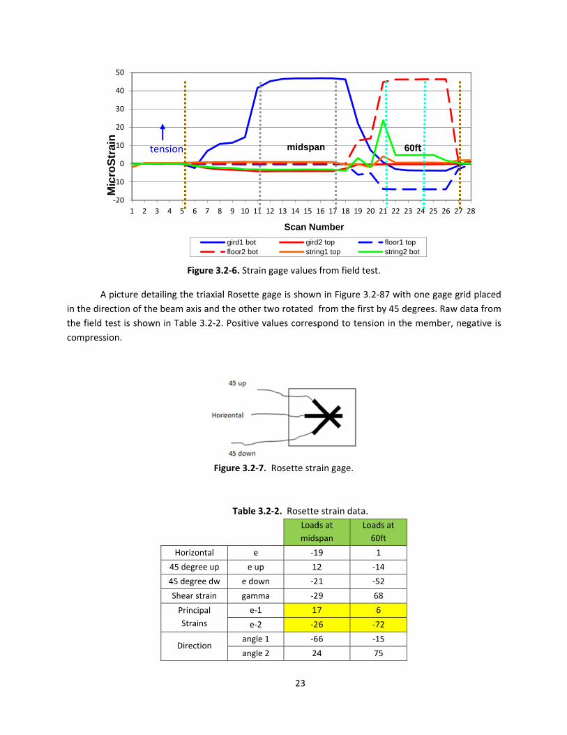
A

in the dire

the field t

compress

picture deta

ection of the

test is shown

sion.

‐20

‐10

0

10

20

30

40

50

1 2 3

Mic

roS

trai

n

te

iling the triax

beam axis an

n in Table 3.2

Horizonta

45 degree u

45 degree d

Shear strai

Principal

Strains

Direction

Figure

4 5 6 7

nsion

xial Rosette g

nd the other t

‐2. Positive v

Figure 3.2‐7.

Table 3.

l e

up e up

dw e dow

n gamm

e‐1

e‐2

angle

angle

e 3.2‐6. Strain

8 9 10 11

gird1 botfloor2 bot

23

gage is shown

two rotated

values corresp

. Rosette stra

.2‐2. Rosette

Load

mids

‐1

12

n ‐2

a ‐2

17

‐2

1 ‐6

2 24

n gage values

12 13 14 15 1

Scan Nu

girdstrin

midspa

n in Figure 3.

from the first

pond to tens

ain gage.

e strain data.

ds at

span

Lo

6

9

2

1

9

7

6

6

4

from field tes

16 17 18 19 20

umber

2 topng1 top

an

2‐87 with on

t by 45 degre

ion in the me

ads at

60ft

1

‐14

‐52

68

6

‐72

‐15

75

st.

0 21 22 23 24

floor1 topstring2 bot

60ft

e gage grid p

ees. Raw data

ember, negat

4 25 26 27 28

placed

a from

tive is

W

the direct

angle for

direction

horizonta

Figure 3.2

With the three

tion and mag

the principa

of principal

l.

2‐8. Direction

midspan

e linearly ind

gnitude of pr

al direction

stresses is s

n of principal

(Position 1) a

dependent st

rincipal stress

is measured

shown in Fig

stresses at gi

and (b) trucks

24

rain measure

ses/strains w

from the h

gure 3.2‐8 wi

(a)

(b)

irder‐knee po

s at 60 ft. from

ements, and

was calculated

orizontal. Gr

ith the princ

oint under loa

m south abut

using Mohr’s

d as shown in

raphical repr

cipal compre

aded dump tr

ment (Positio

s Circle equa

n Table 3.2‐2

resentation o

ssion at 75o

rucks. (a) Truc

on 2).

ations,

2. The

of the

from

cks at

25

3.3 Mirror Lake: Development of Three Dimensional Finite Element Model.

To predict the bridge structural response, an initial three‐dimensional finite‐element‐model

(3DFEM) was created according to the design plans. The 3DFEM model of the bridge was created using

the commercial CSiBridge software.

After the field test was concluded, the truck loading scheme from the field test was replicated

on the analytical model. By comparing the measured strains from the 3D FEM model and the field test,

an evaluation of the model’s accuracy was attained. The analysis results did not match the measured

data as expected. The plans for the bridge were further examined and particular details such as the

support conditions and the degree of composite action between deck and beams were evaluated and

modified.

With the revised analytical model the accuracy was again be verified, and then oversize‐

overload loads (simulating known OSOW vehicles) were applied to the analytic model to evaluate the

actual bridge performance. Then, critical members with high stress to capacity ratios were identified.

Those were then recommended as the members to consider in the issuing of permits for future OSOW

vehicles.

Initial Model Development

Frame, shell and link elements were used to model different sections of the Mirror Lake Bridge.

The selection of these elements was done after considering the advantages of every element type in

modeling.

Floor beams, stringers, bracing elements and the girders were modeled using frame elements.

Detailed modeling of the connections and bolts was not done. Instead, connections between these

members were simulated. Links with different directional stiffness, as explained by Chung and Sotelino

[3], are effective especially for linking the deck and the flexural members for composite action. Links

were necessary since individual members, such as the stringer and floor beam, had their centroids at

different locations so they could not be joined directly. Frame elements were used for the girders and

slant legs. At the knee joint the girder and leg frame elements were assumed to join where their

centroids coincided. This assumption will underestimate the joint stiffness. An alternative would be to

assume the slant leg portion between the bottom of the girder and girder centroid to be rigid. The

concrete deck was modeled using thin shell elements. Bridge geometry was taken from WisDOT design

and shop drawings [10].

In the initial model, the concrete deck to stringer, and concrete deck to floor beam connections

were assumed to be rigid in flexure assuming full composite action. Even though studs were not

provided on portions of the members, under low loading it was suspected that friction would be

sufficient to provide composite action. Links were applied throughout the whole bridge over the

stringers and floor beams. However, for the girders links were only used in the positive moment regions

since ther

connectio

direction.

girder co

centroids

Th

stringers

connectio

like the 3

where th

further. T

The deck

bending. T

the beam

between

Su

bottom o

was mode

modeled

1.

re were no s

ons were mod

These links w

nnection and

of each mem

he floor beam

were attach

on would be c

30” floor bea

e flexural me

The composit

develops ten

The joint betw

connection i

beam and gir

upport restra

f the slant leg

eled using a r

by using a pin

Figure 3.3

studs over a

deled by usin

were defined

d stringer to

mber.

ms were attac

ed to the flo

considered as

m, a full dep

ember is com

e action is ac

sion (under n

ween two co

s considered

rder and betw

aints were a

gs. The conne

roller support

nned connect

3‐1. Initial ext

substantial le

ng fixed linear

d from the ce

o floor beam

ched to the gi

oor beams b

s “pin ended”

pth web conn

mposite with

chieved by tr

negative mom

mposite flexu

as pinned an

ween stringer

pplied over

ection betwe

t. The joint be

tion. A pictur

ruded 3‐D M

26

ength of the

r links, rigidly

ntroid of eac

m connection

irders throug

by bolted ful

” with no mom

nection will p

a deck the

ransferring sh

ment) and the

ural members

nd the deck is

and beam to

the abutmen

een girder and

etween the s

e of the initia

odel of Mirro

element.

girder in the

y linking disp

ch member. In

, rigid links

h full depth w

l depth web

ment resistin

provide some

character of

hear through

e beam has co

s will automa

s continuous.

o simulate a p

nts at the en

d the abutme

slant leg and

al extruded m

or Lake Bridge

e negative m

lacement and

n the case of

were also u

web plates as

b plates. Nor

g capacity. O

e moment ca

f the joint m

the deck to

ombined axia

tically simula

End flexure r

pin end conne

nds of the g

ent, a rocker

the foundatio

model can be

e. Girder mod

oment zones

d rotation in

f the floor bea

used betwee

s noted earlie

rmally a web

n a deep mem

apacity. In a

ust be consid

beam conne

al compressio

ate this condit

releases were

ection.

girders and a

and bearing

on, a true pin

seen in Figur

deled as fram

s. The

every

am to

n the

r. The

b only

mber,

a case

dered

ection.

on and

tion if

e used

at the

plate,

n, was

re 3.3‐

e

27

Comparison with Field Strain Measurements

The results obtained from the initial model are compared with the measured data in Table 3.3‐1

for strain data. Positive values indicate tension and negative compression.

Table 3.3‐1. Strain data comparison between field data and 3‐D model values.

TRUCKS AT MIDSPAN MODEL GAGES

Moment (kip‐ft.)

Axial (kip)

Inertia (in4)

Area (in2)

Stress (Ksi)

Micro‐Strain Micro‐Strain

Floor Beam

Top ‐0.23 ‐0.17 5360 36.5

0.00 0 0

Bottom ‐0.01 0 0

Stringer Top

‐0.01 ‐0.21 1480 20 ‐0.01 0 1

Bottom ‐0.01 0 ‐3

Girder Top

700 ‐4.64 88493 90 ‐3.23 ‐111 ‐4

Bottom 3.13 108 46 Note: Moment, Axial, Inertia, Area and Stress listed on tables are based on the values found in the CSiBridge Model.

TRUCKS AT 60 FT MODEL GAGES

Moment (kip‐ft.)

Axial (kip)

Inertia (in4) Area (in2)

Stress (Ksi)


Floor Beam

Top 37.5 38.4 5360 36.5

0.21 7 ‐14

Bottom 1.89 65 46

Stringer Top

0.63 2.6 1480 20 0.09 3 1

Bottom 0.16 6 5

Girder Top

‐80.5 ‐5.3 88492.5 90 0.31 11 ‐0

Bottom ‐0.42 ‐15 ‐4

Note: Moment, Axial, Inertia, Area and Stress listed on tables are based on the values found in the CSiBridge Model.

As evident from the tables, the model results did not match the data obtained from the field

test. When the trucks are located at midspan, modeled strains on the main girder are significant greater

than the ones obtained from the gages. It can also be seen that composite action is not working

between the concrete deck and girder since the model strain values show that the neutral axis is located

near mid depth of the girder element. Better results were obtained when the trucks are located at 60 ft.

from the south abutment. Floor beam and girder data obtained from the model get closer to the field

values.

Since the girders and columns were approximately modeled as frame elements joining where

their centroids coincide, stresses around the girder knee region could not be accurately attained and a

refinement of the model was done.

Adjustme

Th

the initial

Sotelino,

accurate r

A

only the p

5 ft. wer

composite

Fi

roller sup

This comp

upwards w

and realiz

produce a

nt to the Mod

he first chang

l model the

E. [3]. An at

results by usi

nother refine

positive mom

re defined in

e action due t

inally, joint r

port a new e

pression only

whenever it i

zing that a h

an uplifting of

Figure 3.3‐2.

del Based on

ge in the mod

main girders

ttempt to mo

ng finite elem

ement in the

ment regions h

n the negativ

to the friction

estraint betw

lement was i

element call

s necessary. T

eavy live loa

f the support

. 3D FEM of t

elements

Closer Examin

del was the t

were mode

odel the gird

ment meshing

model was t

had links betw

ve moment

n contact bet

ween the gird

ntroduced w

ed a “gap” [5

This was don

ad at the mid

s. Figure 3.3‐

he Mirror Lak

s, flanges and

28

nation of Des

ype of eleme

led as frame

ers with fine

g.

the location

ween the gird

region cons

ween those t

der and the a

ith the purpo

5] acted as a

e after lookin

dpsan of the

2 displays the

ke Bridge. We

d stiffeners as

sign Details

ent that it wa

e elements as

e shell eleme

of the comp

der and the c

idering that

two surfaces.

abutment wa

ose of only re

roller suppor

ng closely the

bridge, with

e new model

eb of the mai

s frame eleme

as used to mo

s suggested

ents was don

osite links. In

concrete deck

in reality th

as changed.

straining dow

rt but with th

e support in th

hout includin

with the app

n girders defi

ents.

odel the girde

by Chung, W

ne to obtain

n the initial m

k. Now, links

here is a pa

Instead of us

wnward defle

he ability to d

he bridge fiel

g dead loads

plied changes

ined as thin s

ers. In

W. and

more

model

every

rtially

sing a

ction.

eflect

d test

s, can

.

shell

29

The results obtained after implementing the changes described above are shown in Table 3.3‐2.

The girder row in the table does not contain any values in moment, axial, inertia and area cells since

now we are using fine shell elements. The software provides these values only for frame elements. In

the case of shell elements, stress values are taken directly from the software. A positive value denotes

tension in the member and negative compression.

Table 3.3‐2 Strain values measured and predicted.

TRUCKS AT MIDSPAN MODEL GAGES

Moment (kip‐ft.)

Axial (kip)


Stress (Ksi)


Floor Beam

Top ‐0.0735 ‐0.159 5360 36.5

0.00 0 0

Bottom ‐0.01 0 0

Stringer Top

0.1102 0.342 1480 20 0.01 0 1

Bottom 0.02 1 ‐3

Girder Top

Not output by model ‐0.90 ‐31 ‐4

Bottom 3.50 121 46


TRUCKS AT 60 FT MODEL GAGES

Moment (kip‐ft.)

Axial (kip)


Stress (Ksi)


Floor Beam

Top 69.5029 84.232 5360 36.5

0.75 26 ‐14

Bottom 3.86 133 46

Stringer Top

0.729 0.488 1480 20 ‐0.02 ‐1 1

Bottom 0.06 2 5

Girder Top

Not output by model 0.05 2 0

Bottom ‐0.69 ‐24 ‐4


Some improvement can be seen with respect to the first approximate initial model. The floor

beam and girder show composite action and values are closer to the data from the field. However, there

is still big difference in results and the adjusted analytic model does not provide satisfactory results.

Regarding triaxial data obtained, the comparisons with the results from the FEM model are also

unsatisfactory. Table 3.3‐3 shows the values predicted versus the measured ones. Positive values

indicate tension and negative compression.

30

Table 3.3‐3. Triaxial data predicted vs measured.

Values from triaxial

gage

Values from CSiBridge

Model

Loads

Midspan

Loads at

60ft

Loads

Midspan

Loads at

60ft

Max

Strains

ε1 17 6 17 ‐51

ε2 ‐26 ‐72 ‐8 ‐89

Note: Values in microstrain.

Strain data when both trucks were located at midspan get closer to the ones obtained in the

field test. Results when the trucks were located at 60 ft. from south abutment differ with the ones

calculated from the triaxial gages. Orientation of the principal directions was also off as seen in Table

3.3‐4. Since the model is not accurate enough it was not possible to continue the experimentation with

the OSOW vehicles. Development of an improved model is left for future research work.

Table 3.3‐4. Orientation of principal strains.

Principal direction

derived from triaxial gage

Principal direction derived

from CSiBridge Model

Loads

Midspan

Loads at

60ft

Loads

Midspan

Loads at

60ft

Direction ‐66 ‐15 ‐80 ‐44

24 75 10 46

Note: Values in degrees.

Three completely separate models of the Mirror Lake bridge were built using the CSiBridge

software. In one model all of the structural elements were modelled using frame or beam elements,

except the concrete deck was modelled with shell elements. This approach was simple, but an

approximation since the actual rigid frame members were replaced by 1 dimensional linear elements

placed at the centroids of the actual frame members. Where the legs and top girder of the frame

members joined, very deep sections existed, and the joint region was poorly modelled with the

overlapping beam elements. In the other two models the main rigid frames were completely modelled

using shell elements. There was no overlap in the leg to girder connection region.

Unfortunately none of the models were successful in simulating the types of strains that were

actually measured during the load testing. Part of the inaccuracy was contributed by composite action

between the structural framing members and the composite concrete bridge deck. This seems apparent

in the girder strain data listed in Table 3.3‐2 with the trucks at midspan. The predicted girder strains are

much larger than measured. Horizontal thrusts from the leg reactions of the rigid frame, acting a bit like

31

an arch, should be causing high compressive strains in the girder. But the actual data shows small strains

with the model values somewhat higher. The only explanation for the low strains is a good portion of

that compressive thrust is being resisted by the bridge deck even though only a midspan portion of the

girder has a designed composite connection with the deck.

Since the errors in model accuracy were not satisfactory, the results of OSOW truck loading

analyses that were conducted on the Mirror Lake bridge will not be provided here.

4.1 Marin

Th

Marinette

Marinette

that can b

Th

bridge, th

Lift Trunn

main com

back alon

front edg

bascule g

power, th

concrete

bascule b

C

vertical sh

rolling lift

mechanis

nette: Introdu

he Marinette

e, Wisconsin.

e, WI. and 1st

be temporaril

hree types o

he rolling lift t

nion bascule,

mponents of a

g a fixed rack

e of the pier

irder rolls ba

he dead weig

and is locate

ridges) it is lo

Figure 4.1

enter locks a

hear between

t bascules a

ms. Based o

4. M

uction and St

e Bridge, B‐3

. Designed bt St. in Meno

y removed by

of steel bascu

trunnion and

also called “S

a Scherzer rol

k (using elect

r to increase

ck 9ft. when

ght of bascu

ed below the

ocated above

1‐1. Double le

re used to al

n the two lea

re character

on the tong

MARINETT

ructural Com

8‐16, is a do

by the Michi

minee, MI. B

y having one

ule bridges a

the Rall basc

Scherzer” roll

lling bascule.

tric motors) w

the navigabl

in the full op

le leaf is cou

e deck of th

the deck.

eaf Rolling Ba

Structures

llow the leafs

ves and to as

ized by havi

gue‐in‐groove

32

TE BASCUL

mponents

ouble leaf Ba

gan DOT an

Bascule bridge

or two mova

re found in

cule type. The

ing lift due to

It raises the

while the trea

e width of th

pen position.

unterbalance

he bridge, alt

ascule Bridge

Inspection M

s to share loa

ssure proper

ng a fixed c

e principle, t

LE BRIDGE

scule Bridge

d built in 19

es have the f

able spans

modern desi

e Marinette B

o its creator i

leaf by rotat

ad rolls along

he water bod

To make lifti

ed. The coun

though in so

configuration

Manual.

ad resistance

lateral and v

center lock r

the center l

over the Me

973, it conn

flexibility of p

gn: the fixed

Bridge corres

in 1894. Figu

ting the pinio

g the track, re

dy. In the Ma

ng the bascu

nter weight is

ome cases (ty

n. Reprinted f

e. They are re

vertical alignm

replacing mo

lock consists

enominee Riv

ects Ogden

providing cros

d‐trunnion ba

sponds to a R

re 4.1‐1 show

on, forcing it t

etreating from

arinette bridg

le easier, wit

s usually ma

ypically single

from WisDOT

equired to tra

ment. Sherzer

otor‐driven lo

s of a protr

ver in

St. in

ssings

ascule

Rolling

ws the

to roll

m the

ge the

th less

de of

e leaf

T

ansfer

r‐type

ocking

ruding

horizonta

end of the

Th

the bridge

due to th

vehicular

Wheneve

reaction a

the mome

Th

Deck wid

5.67‐ft. w

A picture

Th

bridge len

on a tota

from the

replacem

after first

expansion

l tooth on th

e other leaf [8

he function o

e leaf from ro

he unbalance

live load from

r a vehicle is

and the tail b

ent from live

he Marinette

th is 30 ft. c

wide sidewalk

of the bascul

Figure 4

he bridge ha

ngth. Besides

l of 5 transve

original pla

ent plans are

t construction

n joints.

he end of one

8].

of the live loa

otating down,

ed live load,

m the bascule

s on the leaf,

beam needs a

loading near

e Bridge has a

covering two

on both side

es being lifte

4.1‐2. Marine

s two main b

the two basc

erse floor bea

ans of the s

e shown in F

n involved str

e leaf, which

ad bearing (ta

, when large l

is applied by

e to the appro

the track an

a downward r

the mid‐joint

a total span le

traffic lanes

es. The opera

d is shown in

tte Bridge (W

Reprinted

bascule girde

cule girders, t

ams per leaf

structure, fra

Figure 4.1‐3 a

ringer replace

33

is designed

ail lock/tail b

live loads are

y the tail loc

oach span wh

nd treads act

reaction. The

t.

ength of 143 f

in opposite

tor’s house is

n Fig. 4.1‐2 wi

Wisconsin, HIS

d from Bridge

ers that vary

there are 8 st

running perp

aming plan a

and a structu

ement, paint

to fit into a

beam) is to p

e present on t

k to the app

hen the leave

s like a roller

e couple from

ft. Each lift sp

directions. E

s located on t

th the south

S ID: B38016,

Hunter.com

in depth wit

tringers runni

pendicular to

and cross‐se

ural photo in

ting, overlay

horizontally s

revent the ta

the bridge. An

proach span

es are in the c

r support wit

m these two

pan of the br

Each lane is

the right side

leaf on the le

Bascule bridg

th a paraboli

ing in the lon

the girders.

ctional view

4.1‐4. Majo

concrete wo

slotted jaw o

ail from rising

n upward rea

beam transfe

closed positio

th only an up

reactions bal

idge extends

15‐ft. wide w

e of the south

eft.

ge, span = 14

c shape alon

ngitudinal dire

An elevation

from 1995

r work perfo

rk and clean

on the

g, and

ction,

erring

on [8].

pward

ances

66 ft.

with a

h leaf.

3 ft.).

ng the

ection

n view

deck

ormed

ing of

FFigure 4.1‐3.

Cross secti

Marinette Bri

onal view (ha

idge plans. (a

alf of the brid

34

(a)

(b)

(c)

a) Elevation vi

ge). Adapted

iew with Nort

d from WisDO

th to right (b)

OT HSI databa

) Framing pla

se [10]

n. (c)

Structural

Th

stringers,

of the ma

Th

the web p

are provi

additiona

These pla

girder’s d

to the pie

in Fig.4.1‐

Fl

Floor bea

flange). T

Figure4.1‐4

l Components

he main stru

and bracing

in steel struc

he plate gird

plate. To avo

ded approxim

l cover plate

ate girders ha

epth varies fr

er). An origina

‐3a and b.

loor beams a

ms webs are

The stringers

4.ViewofMt

s

uctural mem

are all made

ctural membe

ers on this b

id local web

mately every

es typically 14

ave a variabl

rom 48 in. at

al plan showin

nd stringers a

connected to

are alternate

Marinetteframheopenend

mbers of the

of steel conf

ers can be see

bridge are bu

buckling, ver

y 3.5 ft. alon

4 in. by 0.5 i

e section thr

floor beam N

ng the beam

are common

o the plate gir

ely continuou

35

mingfrombeofthebascu

bridge are

forming to AS

en in Table 4.1

ilt up from a

rtical stiffene

ng the girder

in. are rivete

roughout the

No. 5 to 126 i

numbering a

W‐shape sec

rder through

us over the flo

elowleafandulegirder.

made of ste

STM designat

1‐1.

angles and fla

rs (typically d

rs as shown

ed on top of

eir span, vary

in. at floor be

nd side view

ctions with co

bolts and a s

oor beams –

djointlockin

eel. The gird

tion A709 gra

ange plates r

double angle

in Figure 4.

the flanges

ying depth an

eam No. 1 (w

of the plate

onstant sectio

stub bracket (

– that is one w

ngmechanism

ders, floor be

ade 36. A sum

iveted togeth

s, 2L 3½ x 5

1‐5. Furtherm

in required z

nd thickness.

with 1 being c

girder can be

on along thei

(below the bo

will be contin

mat

eams,

mmary

her to

x 5∕16)

more,

zones.

. The

losest

e seen

r axis.

ottom

nuous

36

over one floor beam and then simply supported on two others while the adjacent stringer is continuous

over an alternate floor beam. Stringers are thus broken once or twice depending on the stringer. The

stringers sit above the floor beams and their top flange is bolted to the steel metal deck and the bottom

one connected to the floor beam flanges by bolts. This layout is apparent in Figure 4.1‐6.

Lateral bracing is provided with a cross‐bracing formed by structural angles along the bridge

axis. Both the vertical and lower lateral bracing are connected to the girders by bolts, both used to

prevent lateral torsional buckling of the girders.

Table 4.1‐1. Main structural elements description and dimensions.

Member Name Type Dimension

Girder Plate girder with parabolic shape Variable Section

Floor beams Simple span W‐shapes from cl to cl of

girders, spaced at 14ft‐3in

W36x182 (F.B. No. 2 to 4)

W33x220 (F.B. No.5)

Stringers Simple spans W‐shape framed on top of

the floor beams, spaced at 4ft W16×36

Lower Lateral

bracing

X pattern structural angles connecting the

two girders

L 6 x 3½ x 3∕8

L 4 x 3½ x 3∕8

L 3½ x 3 x 3∕8

Side Walk C‐shape channels connected to top of the

bascule girder

12 C 30

15 C 33.9

Counter‐Weight

trusses

Combination of Tee sections and double

angles supporting the concrete counter‐

weight

ST 4 WF 24

ST 5 WF 16.5

ST 6 WF 39

2L 7 x 4 x 5∕8

2L 8 x 8 x 3∕4

2L 4 x 3½ x 3∕8

Th

fastened

flooring is

he deck of e

to the string

s shown in Fig

Figure 4.1

va

Figure 4

each leaf is a

gers with sta

g. 4.1‐7.

1‐5. Bascule G

riable cross s

4.1‐6. Marine

a galvanized

ainless bolts

37

Girder view. St

section along

ette ‐ alternat

5‐in. steel op

approximate

tiffeners ever

the bridge.

te supports fo

pen welded

ed every 1 ft

ry 3.5 ft. and

or stringers.

grid flooring

t. A picture d

a

(ASTM A36)

detailing the

). It is

deck

4.2 Marin

A

critical m

the qualit

oversize/o

Selection

A

chosen fo

between

gages. Th

where the

nette: Field Lo

field test of

embers. Thes

ty of the m

overweight ve

of Test Locat

fter running

or gage place

floor beam N

he tail beam w

e gages were

Figu

oad Testing

the bridge, w

se strains we

odel. The an

ehicles on thi

ion

a prelimina

ement. The

No. 2 and 3,

was instrume

placed.

ure 4.1‐5. 5‐in

with stationar

ere compared

nalytical mod

is bridge.

ry analytical

east bascule

and the floo

ented using tr

38

n. steel open

ry truck loadi

d to predicted

del was then

model of th

girder on t

or beam No.

riaxial gages.

welded grid f

ng, was cond

d strains from

n used to ca

he structure,

he south lea

5 were inst

Figure 4.2‐1

flooring.

ducted to obt

m an analytic

alculate the

, three critic

af of the brid

rumented us

1 shows a sid

tain strain da

cal model to

effects of va

cal locations

dge (Figure 4

sing uniaxial

e and plan vi

ata for

verify

arious

were

4.1‐3)

strain

ew of

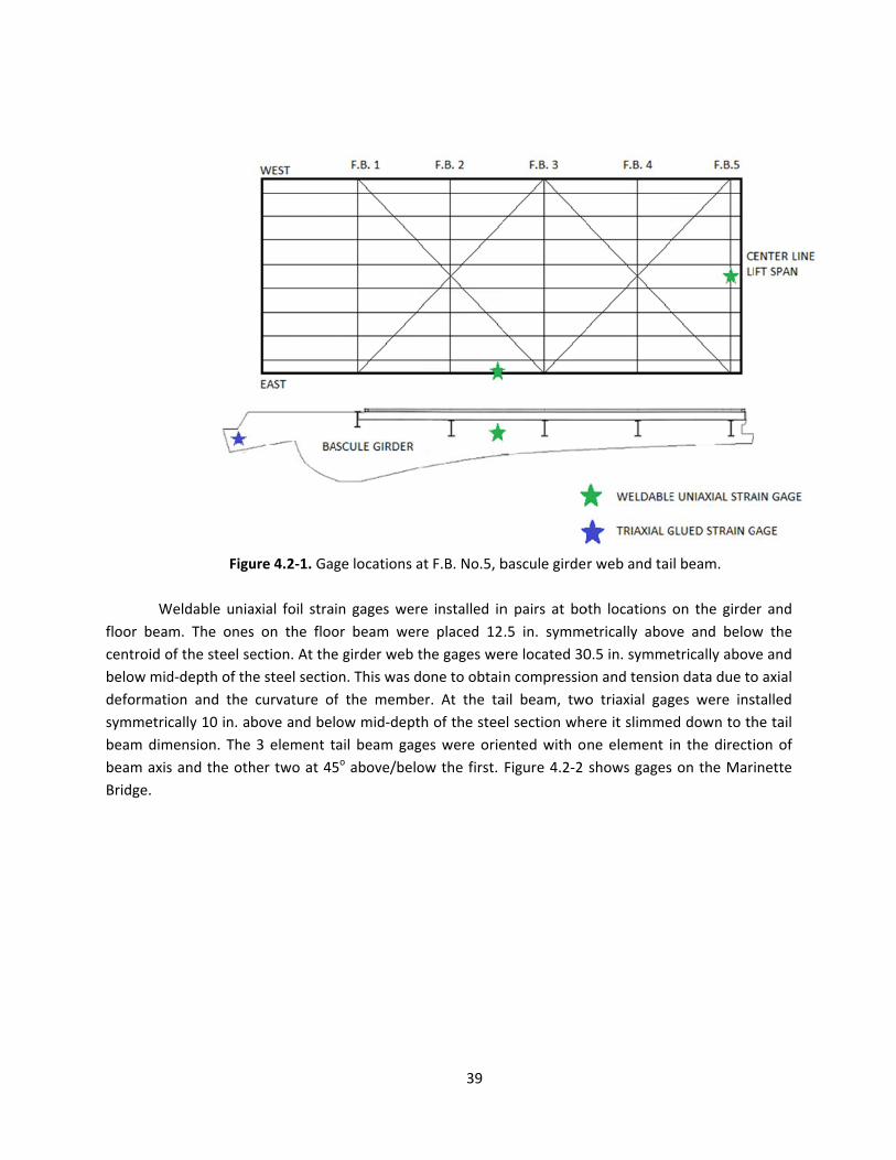
W

floor bea

centroid o

below mid

deformat

symmetri

beam dim

beam axis

Bridge.

Figu

Weldable unia

m. The ones

of the steel se

d‐depth of th

ion and the

cally 10 in. a

mension. The

s and the oth

ure 4.2‐1. Gag

axial foil stra

s on the floo

ection. At the

e steel sectio

curvature of

bove and bel

3 element t

her two at 45

ge locations a

in gages wer

or beam wer

e girder web t

on. This was d

f the membe

ow mid‐dept

ail beam gag

5o above/belo

39

at F.B. No.5, b

re installed in

re placed 12

the gages we

done to obtai

er. At the ta

th of the stee

ges were orie

ow the first.

bascule girde

n pairs at bo

.5 in. symme

ere located 30

n compressio

ail beam, two

el section whe

ented with o

Figure 4.2‐2

r web and tai

oth locations

etrically abov

0.5 in. symme

on and tensio

o triaxial gag

ere it slimme

ne element i

shows gages

il beam.

on the girde

ve and below

etrically abov

n data due to

ges were ins

ed down to th

in the directi

s on the Mari

er and

w the

ve and

o axial

stalled

he tail

ion of

inette

Figur

centerli

No.2 tow

B

behavior

using a t

between

were plac

of the mi

pattern o

re 4.2‐2. Loca

ine of the brid

wards centerl

ehavior of th

of the bridge

total station.

the two leav

ced on sides o

id‐joint conne

n either side

(a

tion of gages

dge. (b) Uniax

line of lift spa

end (tail be

he mid‐joint

e. Therefore, t

The purpos

ves due to lac

of the joint. T

ection. The o

of the joint. F

a)

for field test

xial strain gag

an. (c) Triaxial

eam bearing o

connection i

the deck elev

e of using t

ck of tightnes

Two of them

other two we

Figure 4.2‐3 c

40

(c)

. (a) Uniaxial

ges at bascule

l glued strain

on approach s

in bascule br

vations on eit

the total stat

ss in the joint

were placed

ere place on

clarifies the lo

weldable stra

e’s girder web

gages at tail

span is at top

ridges was a

ther side of th

tion was to

t. Four target

on top of the

top of the e

ocation of the

(b)

ain gages at f

b, 65.375 in. f

beam, 21.5 in

p right).

also of intere

he joint sectio

detect relat

ts for the sur

e west girder

east girder, fo

e targets.

floor beam #5

from floor be

n. from tail be

est in definin

on were mea

tive displacem

rveying equip

r, one on each

ollowing the

5,

eam

eam

ng the

sured

ments

pment

h side

same

Loading R

A

stationary

recorded

and both

weighed 1

Th

interest. F

and the b

the bridge

beam (No

F

Regime

loaded Cou

y live load on

before the te

the mid and

19,140 lbs. an

he location o

First, the reac

back half on t

e. Subsequen

o. 5). Figure 4

igure 4.2‐3. D

nty dump tr

n the bascule

esting. For th

d back axles

nd both the b

of the trucks

ch‐all truck w

he same leaf

ntly, the dum

.2‐4 shows th

Deflection tar

uck (DT‐A) a

e bridge. The

e reach‐all tr

21,000 lbs. (

back axles 18,

s was intend

was located w

. This was do

mp truck was

he exact locat

41

rget locations

nd a reach‐a

weights of t

ruck, the heav

(the fourth a

590 lbs. (the

ed to create

with its front a

ne to obtain

also added w

tion of the tru

(a)

s during the b

all truck (UB‐

he front and

vier one, the

axle was lifte

mid axle was

e the highest

axle on top o

high strain v

with its back

ucks during th

bridge test.

‐60) were us

back axles o

e front axle w

ed). The dum

s lifted).

t stresses on

f floor beam

alues in all th

k axle on top

he field test.

sed to impos

of each truck

weighed 21,88

mp truck fron

n the membe

No. 5 (south

he gages plac

of the same

se the

were

80 lbs.

t axle

ers of

leaf),

ed on

e floor

Gage Inst

Tw

LWK‐XX‐W

Sokki Ken

tail beam

Fo

welding. F

paper, a s

surface th

primer w

recapitula

performa

Fig

provided by

shown in th

tallation

wo types of g

W250B‐350 ¼

nkyujo WFRA‐

. Both installa

or the Micro

First, the zon

smoother sur

he gage was

was applied t

ates this pro

nce beyond t

ure 4.2‐4. Tru

y the county.

he figure. Rea

gages were us

¼ inch strain g

‐6‐11 0.43 in

ations were p

o‐Measureme

e was ground

rface was obt

spot welded

to the groun

ocess on the

the load test.

ucks used on

(b) Location

ch‐all Truck n

the w

sed for strain

gages were in

ch waterproo

previously fea

ents weldable

d to remove t

tained and a

to the steel

nd area and

Marinette B

42

(b)

the field test

of the trucks

next to the ea

west bascule g

n analysis on t

nstalled on flo

of 3 element

atured in Figu

e uniaxial ga

the paint unt

lcohol was a

element usin

to the gage

Bridge. Thes

t. (a) Reach‐al

in the South

ast bascule gi

girder.

the Marinett

oor beam No

t strain gage

re 4.2‐2.

ges, the inst

til the steel su

pplied to clea

ng a Sunston

e to prevent

e gages wer

ll Truck and D

leaf. Lifted ax

rder, dump tr

e Bridge. Mic

o. 5 and the g

rosettes wer

tallation invo

urface was ex

an the area.

e Pulse Tack

t steel corro

re not inten

Dump Truck

xles are not

ruck next to

cro‐Measurem

girder web. T

re installed o

olved grinding

xposed. With

Then with a

Welder. Fina

sion. Figure

ded to rema

ments

Tokyo

on the

g and

h sand

clean

ally, a

4.2‐5

ain in

F

insta

Th

surface is

alkaline/a

Lastly, pri

4.2‐6 show

igure 4.2‐5. W

allation. (b) S

he 3‐element

s ground to e

acidic surface

imer is applie

ws a rosette s

(a)

Weldable unia

train gage we

t strain gage

expose the st

cleaners. Cy

ed to the grin

strain gage us

axial strain ga

elded after su

rosette is th

eel web. The

yanoacrylate

nd surface an

sed on the ta

43

(c)

ages on Marin

urface was cle

he same type

en, the surfac

glue is used

nd to the gag

il beam of the

nette Bridge.

eaned. (c) Pri

e used in the

ce is cleaned

to place the

ge to prevent

e Marinette B

(b)

(a) Grinding

mer applied t

e Mirror Lake

with alcoho

e gage on the

t corrosion of

Bridge.

steel web for

to work area.

e Bridge. Firs

l and water‐b

e defined loc

f the steel. F

r gage

.

st, the

based

ation.

Figure

Data Colle

Th

the bridge

begin. The

stage one

bridge. In

on top of

as well as

locations

CSiBridge

girder, an

location o

the bridge

In

using the

readings.

St

two and t

could be

load.

ection Schem

he installed s

e operation c

e County clos

e, an initial re

stage two, t

floor beam N

s the readings

with respect

analytical m

nd the UB‐60

of the axles w

e.

n addition to

e total statio

tage one and

three were t

compared w

F

e and Results

strain gages o

ontrol room.

sed the bridge

eading of all t

the reach‐all

No. 5. The stra

s taken from

t to the east

model. In stag

0 stayed in p

were taken. Fi

the strain da

n. Each targe

d four were d

then adjusted

ith the strain

igure 4.2‐6. T

s

on the bridge

After getting

e and detoure

the gages and

(UB60) truck

ains under th

the deflectio

t girder were

ge three, the

lace. Again,

inally, in stag

ata gathered

et was meas

one to estab

d by the base

ns found in th

44

Triaxial strain

were connec

g initial readi

ed the traffic

d midspan de

was driven i

he stationary

n targets. Wh

e recorded in

dump truck

all the data

e four, data w

in every stag

sured once p

lish a base lin

e line readin

he CSiBridge

gage at tail b

cted to a dat

ngs from all t

c. The test pla

eflections was

nto its positi

truck loading

hile taking th

n order to p

was driven i

from the gag

was gathered

ge, the eleva

per load stag

ne reading w

g to determi

analytical m

beam.

ta acquisition

the gages, the

an was divide

s taken with

on, next to t

g were collect

e readings, th

place the truc

nto its positi

ges and targ

d again witho

ation of the m

ge adding up

with no load. R

ine the chan

odel under o

system locat

e test was rea

d in four stag

no vehicles o

he east girde

ted in all the

he exact truc

ck later on i

ion, near the

ets plus the

out any vehicl

mid‐joint was

p to a total

Results from

ge in strain w

only stationar

ted in

ady to

ges. In

on the

er and

gages

k axle

n the

e west

exact

les on

s read

of 16

stage

which

ry live

45

Strain Data

A total of 211 scans were taken during the four stages. The first 60 scans represent the data with

no load on the bridge. The following 50 scans show the data with the reach‐all truck parked on the west

side of the South bascule leaf. The next 50 scans represent the data with the reach‐all truck plus the

loaded dump truck on the east side of the South bascule leaf. The last 60 scans correspond to the data

with no load on the bridge. During each test step the strain gages were read at a scan rate of 2

scans/second. The time to read elevations was approximated 5‐10 minutes, and the strain gage data

was collected at the beginning and end of this period. Strain gage data obtained from the field test was

reliable and consistent with a standard deviation of less than 1 microstrain. The average data obtained

from the uniaxial strain gages on the floor beam and the girder web is shown in the Table 4.2‐1. Positive

values correspond to tension in the member, negative is compression.

Table 4.2‐1. Strain data.

Floor Beam Girder

Top Bottom Top Bottom

Strain due to reach‐all

truck ‐20 20 38 ‐55

Strain due to reach‐all

truck + dump truck ‐48 53 42 ‐63

Note: Values in microstrain already adjusted with base line reading.

As seen in Table 4.2‐1, strain on the floor beam top and bottom increases and more than

doubles in magnitude between stage 2 and 3 of the testing. This was expected since floor beam No.5 is

picking up stresses from both trucks, and they have approximately the same weight.

The same response wasn’t observed with the data from the girder gages. The increment in

microstrain from stage 2 to stage 3 is very small, approximate 12%. This was likewise expected since

these strain gages were located on the east bascule girder. In stage three, the dump truck is located in

the far lane, closer to the west bascule girder. The stresses due to the dump truck are picked up mostly

by the west girder, generating a small increase in strain in the strain gages of the east girder. All the data

gathered on the field test was plotted on the following graphs, Fig. 4.2‐7 for floor beam data and Fig.

4.2‐8 for the girder. Scans 60 to 110, and 111 to 160 represent the data with only the reach‐all truck and

both trucks, respectively.

46

Figure 4.2‐7. Strain gage from floor beam No.5.

Figure 4.2‐8. Strain gage from bascule girder.

The data obtained from the triaxial gages at the tail beam are shown in Table 4.2‐2. Positive

values indicate tension, negative compression. Figure 3.2‐7 in Section 3 describes the notation used for

the triaxial gages and their shape.

‐60

‐40

‐20

0

20

40

60

0 50 100 150 200 250

MicroStrain

ScanNumber

Floorbeamtop Floorbeambottom

‐80

‐60

‐40

‐20

0

20

40

60

0 50 100 150 200 250

MicroStrain

ScanNumber

BasculeGirdertop BasculeGirderbottom

Fr

gathered

29,000 ks

transferri

angles as

bending m

friction be

section co

acting in f

rom Table 4

on the field

si. This could

ng load to th

stiffeners. S

member. In a

etween both

ould create a

flexure this ef

Ta

Top

Bottom

.2‐2 the stra

test. The pea

d be explaine

he approach

Strain data sh

ddition to ve

surfaces ma

stress conce

ffect is of less

Figure 4.2‐

able 4.2‐2. Ro

45 down

horizonta

45 up

m

45 down

horizonta

45 up

Note: Values

with b

ains experien

ak stress rea

ed by the ke

span using a

hows that the

ertical bearing

ay also induce

ntration notc

ser importanc

‐9. Tail beam

47

osette data at

Reach‐

truck

n ‐81

al ‐11

134

n ‐89

al ‐45

72

in microstrain

ase line readin

ced by the

ched a value

ey role that

a complicated

e tail stub is

g force betwe

e stresses in

ch, as illustrat

ce.

m region with

t Tail beam.

‐all

k

Both

truck

‐149

‐29

239

‐167

‐87

138

n already adjus

ng.

tail beam w

e of 7.3 ksi, a

the live load

d built‐up tai

working as

een the two b

the tail bea

ted in Figure

bearing and

h

ks

9

9

9

7

7

8

sted

eb are large

assuming a Yo

d bearing (Fi

il section wit

a shear strut

bearing plate

am zone. The

4.2‐9, but sin

notch.

est of all the

oung’s modu

igure 4.1‐1)

th multiple ri

t rather than

es at the tail b

e abrupt chan

nce the stub

e data

lus of

plays,

veted

n as a

beam,

nge of

is not

48

Figure 4.2‐10. Tail beam top principal strains

Figure 4.2‐11. Tail beam bottom principal strain.

‐50.0

‐30.0

‐10.0

10.0

30.0

50.0

‐250.0‐200.0‐150.0‐100.0‐50.00.050.0100.0150.0200.0

0 50 100 150 200 250

angle(degrees)

microstrain

scannumbermaxstrain minstrain strainangle

‐60.0

‐40.0

‐20.0

0.0

20.0

40.0

60.0

‐200.0

‐100.0

0.0

100.0

200.0

300.0

0 50 100 150 200 250

angle(degrees)

microstrain

scannumbermaxstrain minstrain strainangle

W

Circle equ

Figures 4.

represent

strain occ

for the bo

A

beam is sh

A

angle. The

value of 2

the tail be

cause unu

beam reg

just the re

Th

diagonal

With the three

uations, the

.2‐10 for the

t the principa

curs was also

ottom one ‐13

graphic rep

hown in Figur

Figure 4

s is clear in F

e maximum v

251 microstra

eam is a “dist

usual force flo

ion to produc

egion shown

he strains sho

tension mem

e linearly ind

direction an

top triaxial g

l strains obta

calculated. F

3 degrees (‐ in

resentation o

re 4.2‐12.

4.2‐12 Tail bea

Figure 4.2‐12,

value is tensi

ain (7.3ksi). T

turbed” regio

ow. The FEA

ce exact strai

in Figure 4.2‐

own in the ta

mbers in the

dependent st

d magnitude

gage and 4.2‐

ained from th

or the tail be

ndicating cou

of the princip

am principal

co

, principal str

on and happ

hese strains a

on where the

modelling us

in values. Bet

‐12.

ail beam coul

e web at nea

49

rain measure

e of principa

11 for the bo

he field test d

eam top gage

unter‐clockwis

pal direction

strains phase

mpression.

rains at both

ens at the to

are part of a

reaction, mu

sed for the en

tter strain est

d be interpre

arly 45 degr

ements from

l stresses/str

ottom triaxia

data. The prin

the angle is a

se from the g

and magnit

e 3. Positive s

locations oc

op location ne

complex stra

ultiple stiffen

ntire bridge is

timates woul

eted as resem

ees from ho

Table 4.2‐2,

rains were fo

l gage. Red a

ncipal angle w

approximated

gage axes).

ude of the s

ign is tension

cur at approx

ear the live lo

ain pattern s

ers, and abru

s not sufficie

d require det

mbling a truss

orizontal and

and using M

ound as show

and blue solid

where the pri

d ‐10 degrees

stresses at th

n, negative is

ximately the

oad bearing w

since this reg

upt section ch

ntly fine in th

tailed modell

s mechanism

45o compre

Mohr’s

wn in

d lines

ncipal

s, and

he tail

same

with a

ion of

hange

he tail

ing of

, with

ession

50

diagonals. The four 0.5in. thick angle stiffeners at the end, below the bearing, likely absorb most of the

vertical bearing force and transfer it into the web as the force moves down through the angles along

the web. The downward force transferred from the angles to the web is balanced by the upward

component of the tension diagonal pulling on the angle and the upward component of the compression

diagonal pushing on the angles. The difference in strains between the top gage and bottom suggests

normal beam action with flexural stress is not occurring. The low flexural stress reduced the possibility

that stress concentration will develop at the inner part of the tail beam where the section depth

suddenly starts to increase.

Deflection Data

With the data taken from the surveying equipment, deflections at the four targets on poles

were calculated using trigonometric relationships. The processed data is presented in Table 4.2‐3 and a

key to the target locations was provided in Figure 4.2‐3 (Raw data from surveying equipment can be

found in the Appendix). Stations 1 and 3 were on the loaded bridge leaf and stations 2 and 4 were on

the unloaded opposite leaf. With just the reach‐all truck, the deflections of the loaded leaf were 0.07 to

0.03 in. greater than the unloaded leaf. This difference appears to indicate a certain amount of “play” in

the mid‐joint before load is transferred across the joint. The value at Station 4 under double truck load

(0.81 in.) appears to be unexpectedly high creating doubts on its accuracy. Positive values correspond to

downward deflections.

Table 4.2‐3. Mid‐joint deflections under truck loading.

Deflections (in)

Reach‐all

Truck

Station 1 0.55

Station 3 0.25

Station 2 0.48

Station 4 0.22

Reach‐all

Truck + Dump

Truck

Station 1 0.68

Station 3 0.71

Station 2 0.61

Station 4 0.81

4.3 Marinette: Development of Three Dimensional Finite Element Model.

As described in Section 4.2, an initial 3D FEM was created according to design plans to predict

the bridge structural response. The 3D FEM model of the bridge was created using the commercial

51

CSiBridge software. From this model, critical locations where high strains were expected were identified

as a means of selecting locations to place the strain gages.

After the field test was concluded, the truck loading scheme from the field test was replicated

on the analytical model. By comparing the measured strains from the 3D FEM model and the field test,

an evaluation of the model’s accuracy was attained. The analysis results did not match the measured

data as was expected. The plans for the bridge were further examined and information on particular

details such as the stiffness of the grid deck, the rigidity of connections between flexural members, the

degree of composite action between deck and beams, and the tightness of the midspan joint, were re‐

considered from field observations and were evaluated and modified if there was doubt as to the

accuracy of the first modeling method.

With the revised analytical model the accuracy was again verified, and then oversize‐overload

(OSOW) loads (simulating known OSOW vehicles) were applied to the analytic model to evaluate the

actual bridge performance. Critical members with high stress to capacity ratios were identified. Those

are then recommended as the members to consider in the issuing of permits for future OSOW vehicles.

Initial Model Development

Different elements were used to model different sections of the Marinette Bridge. The selection

of these elements was done considering the advantages of every element type. Frame, shell and link

elements are the most common ones.

Floor beams, stringers, bracing elements and stiffeners, angles and flanges of the two girder

sections were modeled using frame elements (see Table 4.1‐1 for specific member sizes). The steel open

grid deck, girder web and counterweight concrete area were modeled using thin shell elements. Finally,

connections between these members were bolted in reality but detailed modeling of the bolts was not

done. Instead, connections were simulated by links with different directional stiffnesses. The links were

necessary since individual members, such as the stringer and floor beam, had their centroids at different

locations. The links connected the centroid of a stringer, over the floor beam, to the centroid of the floor

beam to resemble the actual geometry as accurately as possible.

Bridge geometry was taken from Michigan State Highway Department design and shop drawings

[10], but the poor quality of the old drawings made understanding of some details difficult. The initial

model was constructed using known member sizes and assumed connection behavior as detailed in the

following.

The bridge stringers were modelled as 2 span frame elements, continuous over the center floor

beam and simple supported at the end floor beams. These model configurations of 2 span stringers

were alternated – with one stringer continuous over a floor beam and the adjacent stringer non‐

continuous.

52

In the initial model, the steel deck to stringer and stringer to floor beam connections were

assumed to be rigid in flexure. A flexural rigid connection implies full composite action. As noted earlier,

the deck was bolted to the stringers at 1ft. intervals making composite action possible. The two

connections were modeled by using fixed linear links, rigidly linking displacement and rotation in every

direction. These links extended between the centroids of each member. The floor beam to girder

connection was assumed to transfer only shear since the actual connection consisted of bolting between

the beam web and a girder stiffener. A link element wasn’t necessary because the floor beam ends

(frame element) and the girder web (shell element) shared the same nodes. End releases were used at

both ends of the floor beam in order to obtain a shear‐only connection.

The bridge’s mid‐joint between bascule leaves was assumed to only allow the transfer of vertical

shear forces between the two leaves. The connection was modeled using partially fixed linear links,

transferring zero moment between leaves but fully transferring any displacements.

The counterweight is a large concrete block with embedded steel truss members. The assumed

rigid behavior of the counterweight was modeled by using very high stiffness values with the concrete

shell areas. No counterweight truss elements were simulated in the model, only the stiff shell areas

connected rigidly to the girder web by sharing the same nodes.

Joint restraints were applied to the bascule girders. The connection between bascule girder and

the pier was modeled assuming that the bascule girder can rotate only about the transverse axis of the

bridge. Vertical movement at the contact point between the “tread” and “track” (see Figure 3.1‐1) was

assumed to be zero and modeled as a pin support. The contact between the tail beam and the approach

span beam was modeled by using a pinned connection, this assumption prevented horizontal and

vertical movement at that point and is based on the assumption that horizontal friction will develop

between the bearing plates. Finally, the bascule pinion was also restricted from displacements assuming

that its stays always in the same place. A picture of the initial analytical model can be seen in Figure 4.2‐

13.

Comparison with Field Strain Measurements

The results obtained from the initial model are compared with the measured data in Table 4.2‐4

for strain and 4.2‐5 for deflection data. Positive values indicate tension, negative is compression.

Figure 4.2

Elemen

Floor

Beam

Girder

Tail

Beam

Note: Mom

Elemen

Floor

Beam

Girder

Tail

Beam

A

Modeled

values an

2‐13. 3D FEM

t Location

Top

Bottom

Top

Bottom

Top

Bottom

ment, Axial, Ine

t Location

Top

Bottom

Top

Bottom

Top

Bottom

Note: Mom

All the meas

strain result

d the error (in

M of Marinette

Tab

RE

Moment

(kip‐ft.)

19.7

ertia, Area and

REACH‐

Moment

(kip‐ft.)

31.2

ment, Axial, Ine

ured strains

s obtained w

n the tail bea

e Bridge. Con

le 4.2‐4 Strain

ACH‐ALL TRU

Axial

(kip)

45.9

Not output

Stress listed o

‐ALL + DUMP

Axial

(kip)

74.4

Not output

rtia, Area and

CSi

and induced

with the reac

m) is equivale

53

crete counte

in cyan.

n values mea

UCK

Inertia

(in4)

12178

t by model

on tables are b

P TRUCK

Inertia

(in4)

12178

t by model

Stress listed o

Bridge Model.

d stresses ar

h‐all truck an

ent to 3200p

rweight show

sured and pr

Area

(in2)

64.1

ased on the va

Area

(in2)

64.1

n tables are ba

re very low

nd both truc

si of stress.

wn in red and

redicted.

M

Stress

(Ksi)

0.47

0.96

0.10

‐0.94

0.70

‐0.56

alues found in

M

Stress

(Ksi)

0.78

1.54

0.12

‐1.15

0.92

‐0.72

ased on the va

values with

cks disagree w

the steel me

MODEL GA

Micro‐

Strain

M

St

16 ‐

33

3

‐32 ‐

24 ‐

‐19 ‐

the CSiBridge

MODEL GA

Micro‐

Strain

M

St

27 ‐

53

4

‐40 ‐

32 ‐

‐25 ‐

lues found in t

the loading

with the me

embers

AGES

Micro‐

train

‐20

20

38

‐55

‐11

‐45

Model

AGES

Micro‐

train

‐48

53

42

‐63

‐29

‐87

the

g used.

asured

54

In terms of deflections, the results obtained with the initial model are shown in Table 4.2‐5. The

positions 1&3 are on the loaded leaf and 2&4 are on the opposite unloaded leaf. Positive values indicate

downward deflection.

Table 4.2‐5. Deflection values at mid‐joint connection.

Deflections (in)

Surveying

equipment

CSiBridge

Model

Reach‐all

Truck

Station 1 0.55 0.47

Station 3 0.25 0.13

Station 2 0.48 0.46

Station 4 0.22 0.13

Reach‐all

Truck + Dump

Truck

Station 1 0.68 0.58

Station 3 0.71 0.58

Station 2 0.61 0.58

Station 4 0.81 0.58

As expected, the deflections at the different stations in our analytical model after the two trucks

were placed on the bridge were the same, 0.58 in. This was attributed to the use of rigid links in

between the two bascules leaves, transferring shear forces from one leaf to the other. A change in the

mid‐joint connection is necessary for more accurate results. Measured results from Table 4.2‐5 show

that the connection between the two leaves is not rigid, considering that the south lift span (locations

#1 and #3) deflected more than the north one (except for the large value of 0.81 in. at location #4 –

which might possibly be an errant data point).

Although the strain values were quite inaccurate and the deflection values differ a little bit from

the ones measured in the field test, the initial model served as a good starting point

Adjustment to the Model Based on Closer Examination of Bridge Details

During the load testing a close inspection was made of the bridge components and connections

that led to needed changes in the analytic model – which was based on poorly preserved original bridge

plans. The first adjustment needed for the model was in the mid‐joint connection between bascule

girders. The original assumption of a complete vertical locking between the two leaves was incorrect.

The degree to which the leaves are locked together depends on a tight adjustment of the bearing plates

in the joint. With repeated traffic these joints are known to become loose and are regularly tightened (at

least annually) as part of the bridge maintenance. To more reasonably model the joint, instead of using

rigid linear links, a hook link element was used. A hook element is a partially linear link element that

transfers

stiffness o

stretched

between

Th

match the

to simulat

gaps, but

maximum

joint is no

There ap

bottom).

A

the string

preventin

joint). A c

are attach

floor beam

restricting

displacem

stringers

beam) wa

tension only

of the link is

more than th

bascule bridg

he hook elem

e difference b

te rigidity onc

with repeate

m forces in th

ot adjusted fr

pears to be

nother refine

gers and floo

ng differentia

close conside

hed to the flo

m) and the u

g relative rot

ments, but no

and the deck

as changed fro

[5]. It can be

s zero. A pre

he defined in

ge leaves.

ment in the m

between the

ce the gap clo

ed loading th

e loaded leaf

requently. Fig

some lack o

Figure 4.2‐

ement in the

or beams. In

l rotations an

ration of the

oor beams by

pper flange o

tation betwe

ot rotations.

k. The connec

om fixed to p

defined with

e‐defined line

itial gap. This

model was de

measured de

oses. Typicall

e gaps in bea

f, might best

gure 4.2‐14 s

of contact be

14. Joint betw

model was a

the initial m

nd displacem

bridge plans

y bolts betwe

of the floor be

een the two

The floor b

ction betwee

partially fixed

55

h an initial op

ear stiffness

s modelling m

efined with a

eflection of th

y the joint is

arings do gro

use a gap op

hows the joi

etween the t

ween leaves o

a change in t

model, this c

ents betwee

s, and inspect

en the lower

eam. It is dou

elements. T

beam will no

n these mem

links, preven

ening betwee

of the link t

may be essent

an initial open

he two spans)

adjusted at l

w again. Con

pening of ¼ i

nt in the brid

tooth (on rig

of Marinette

the assumed

connection w

n the memb

tion in the fie

r flange of the

ubtful whethe

The connectio

ot develop a

mbers (deck t

nting only the

en the two el

takes action

tial in modell

ning of 0.07

) and a very h

east once pe

nservative mo

nch which co

dge at the tim

ght) and the

bascule bridg

connection

was modeled

ers (a shear

eld, revealed

e stringer (wh

er this conne

on should re

ny composit

to stringer an

relative vert

ements wher

after the lin

ing the conne

in. (in this ca

high stiffness

r year to elim

odelling, to p

ould develop

me of load te

bearing plat

ge.

behavior bet

using fixed

and moment

d that the stri

hich sits abov

ection is capa

estrain differ

e action wit

nd stringer to

ical displacem

re the

nk has

ection

ase to

value

minate

redict

if the

esting.

te (at

tween

links,

t rigid

ingers

ve the

ble of

rential

h the

o floor

ment.

A

apparent

stringers.

stringer.

torsion of

action wit

form as th

Jo

roller con

(and frict

Bascule p

(Figure 4.

Fi

elements

block. Cou

a “rigid bo

a more rig

Th

changes d

negative o

fter field insp

that the grid

The T is visi

Shear develo

f the T sectio

th the orthot

he link describ

oint restraint

nnection. Exa

tion) between

pinion was re

1‐1).

inally, the co

originally em

unterweight s

ody constrain

gid behavior.

he results ob

described abo

one compress

pection and

d itself sat on

ible in the fig

oped, for com

on. That sect

tropic grid. T

bed above fo

between th

mination of t

n the bearin

eleased after

unterweight

mployed coul

steel trusses

nt.” These cha

Figure 4.2‐15

Figure

btained with

ove, are show

sion.

observation

n small inver

gure. The bot

mposite actio

tion was judg

The link betw

r the stringer

e tail beam

the tail beam

g plates wou

realizing tha

was redefine

ld adequately

were introdu

anges were ex

5 displays the

e 4.2‐15. (a) E

the refined m

wn in Table 4

56

of the open

rted T section

ttom flange

on, would ha

ged to have

ween stringers

r‐beam conne

and the appr

m during bridg

uld be minim

t the pinion

ed. There was

y simulate th

uced and the

xpected to in

e new model w

(a)

(b)

Extruded mod

model of the

.2.6. A positiv

grid decking,

n purlins tha

of this T is b

ave to be tr

insufficient s

s to the deck

ection.

roach span w

ge inspection

mal. The join

actually mov

s some conce

he rigidity of

whole system

crease the co

with the appl

del. (b) Analyt

e Marinette B

ve value indic

, shown in F

t ran perpen

bolted to the

ransferred to

stiffness to d

king was cha

was changed

n hinted that

t between t

ves horizonta

ern as to whe

f the large re

m was link tog

ounterweight

lied changes.

tic model.

Bridge, after

cates tension

igure 4.1‐5, i

ndicular acros

top flange o

o the grid th

develop comp

anged to the

from pinned

horizontal m

he girder an

ally along the

ether the stiff

einforced con

gether by app

t stiffness, sho

implementin

n in the mem

it was

ss the

of the

rough

posite

same

d to a

motion

d the

e rack

f shell

ncrete

plying

owing

ng the

ber, a

57

Table 4.2‐6 Strain values measured and predicted.

REACH‐ALL TRUCK MODEL GAGES

Element Location

Moment

(kip‐ft.)

Axial

(kip)

Inertia

(in4)

Area

(in2)

Stress

(Ksi)

Micro‐

Strain

Micro‐

Strain

Floor

Beam

Top 72.7 1.8 12178 64.1

‐0.87 ‐30 ‐20

Bottom 0.92 32 20

Girder Top 1.12 39 38

Bottom No output by model

‐2.22 ‐77 ‐55

Tail

Beam

Top ‐0.07 ‐2 ‐11

Bottom ‐0.4 ‐14 ‐45

Note: Moment, Axial, Inertia, Area and Stress listed on tables are based on the values found in the CSiBridge

REACH‐ALL + DUMP TRUCK MODEL GAGES

Element Location

Moment

(kip‐ft.)

Axial

(kip)

Inertia

(in4)

Area

(in2)

Stress

(Ksi)

Micro‐

Strain

Micro‐

Strain

Floor

Beam

Top 156.4 4 12178 64.1

‐1.86 ‐64 ‐48

Bottom 1.99 69 53

Girder Top 1.31 45 42

Bottom Not output by model ‐2.65 ‐91 ‐63

Tail

Beam

Top ‐0.1 ‐3 ‐29

Bottom ‐0.51 ‐18 ‐87

Note: Moment, Axial, Inertia, Area and Stress listed on tables are based on the values found in the CSiBridge

The new predictions are more consistent with the measured data, though not exactly identical.

Floor beam strains at top and bottom are nearly equal, as expected with a non‐composite behavior.

Strains at the girder top location correlated very well with the values obtained in the field, with

differences less than 3 microstrain. However, strain values predicted for the bottom location were

higher than the ones obtained in the field test by 22 to 28 for a 780psi error.

Strain values at the tail beam are not consistent with the data obtained from the model. This is

likely due to the complexity of the region where the gages were placed. This area is highly congested by

angle stiffeners with rivets and an abrupt section change. Moreover, friction between the tail beam

bearings may still induce some stresses on the tail beam. All of these produce a very complex stress

distribution on the tail beam. It is not possible to model this disturbed region with minimum element

size of 10 by 7.5 inches as used in the girder web here. A more refined model, i.e. 3‐D Finite Element

small scale analysis of the isolate area, is required to simulate the actual strains. That will be left to

future research work.

Deflections with the refined model show an improved correlation with respect to the field test

measurements. As seen in Table 4.2‐7, with the introduction of the Hook to model the gap at the

midspan joint, there is a better agreement in deflections at the 4 targets (except for the large value of

58

0.81 at location #4 – which is likely an errant data value since deflections in the unloaded leaf should not

be larger than in the loaded leaf). Positive values correspond to downward deflections.

Table 4.2‐7. Deflection values at mid‐joint connection.

Deflections (in)

Surveying

equipment

CSI Bridge

Model

Reach‐all

Truck

Station 1 0.55 0.55

Station 2 0.48 0.46

Station 3 0.25 0.16

Station 4 0.22 0.13

Reach‐all

Truck + Dump

Truck

Station 1 0.68 0.65

Station 2 0.61 0.56

Station 3 0.71 0.68

Station 4 0.81 0.59

4.4 Marinette: Impact of OSOW Vehicles.

Six dual lane trailers, two single lane trailers and the HL‐93 trucks, as described in Chapter 2,

were analytically driven across the Marinette bascule bridge to measure the vehicle’s force impact. Each

of these vehicles was described earlier along with the geometry of the loaded lanes. Critical members

where high stresses developed were identified. The dead load of the bridge was included in the analysis

for all the load combinations. The response of only principal members, such as stringers, floor beams

and girders, were examined in this project. Joints, bracing, diaphragm and deck members were not

included in the scope. The OSOW vehicle loads are factored by 1.35, HL‐93 by 1.75 and dead load by

1.25. The AASHTO multi‐presence factor is used with the Hl‐93 loads, but no the OSOW load.

The results obtained from the analyses are summarized in Table 4.4‐2. The notation in the tables

for single and dual trailers is as follows and is detailed further in Table 4.4‐1:

Single312 represents the 312 kips gross weight single trailer,


Dual486 represents the 486‐kip gross weight dual trailer,

Dual500 represents the 500‐kip gross weight dual trailer.

Fi

members

second pl

Th

capacity.

driven do

Truck Notat

HL‐93

Single312

Single446

Dual500‐2

Dual500‐6

Dual500‐1

Dual486‐2

Dual486‐6

Dual486‐1

igures 4.4‐1

under movin

ot shows axia

Figure 4.4‐1

Figure 4.4‐2

he flanges o

In Figure 4.4‐

wn the load

Table 4

ion

2

6

2 500 g

6 500 g

0 500 gr

2 486 g

6 486 g

0 486 gr

and 4.4‐2 sh

ng load comb

al force in the

. Moment en

2. Axial force

of the girders

‐2, axial force

lanes. Axial fo

4.4‐1. Notatio

AAS

3

44

ross weight d

ross weight d

ross weight d

ross weight d

ross weight d

ross weight d

how a mome

inations. The

e girder flange

velope of crit

envelope of g

s, under axia

es are plotted

orces in top f

59

on used in res

Desc

SHTO HL‐93 tr

12 gross weig

46 gross weig

dual trailer wi

dual trailer wi

ual trailer wit

dual trailer wi

dual trailer wi

ual trailer wit

ent and axia

first plot sho

es.

tical member

girder flanges

al load, prov

d in every flan

flanges are al

sults of OSOW

ription

ruck combina

ght single trai

ght single trai

ith 2 ft. transv

ith 6 ft. transv

th 10 ft. trans

ith 2 ft. transv

ith 6 ft. transv

th 10 ft. trans

l force enve

ows floor bea

rs under OSOW

s under OSOW

vide most of

nge along the

most entirely

W analysis.

ations

iler

iler

verse wheel s

verse wheel s

sverse wheel

verse wheel s

verse wheel s

sverse wheel

lope for the

am and mome

W/HL‐93 truc

W/HL‐93 truc

f the girder

e girder when

y in tension, e

spacing

spacing

spacing

spacing

spacing

spacing

e different fle

ent envelopes

ck combinatio

k combinatio

moment res

n OSOW truck

except close t

exural

s. The

ons.

ons.

sisting

ks are

to the

60

mid‐joint connection. Bottom flanges are the opposite in compression all along the girder and with

larger values than the top flanges.

Values seen in Table 4.4‐2 were obtained with the axial and bending moment envelopes (as

shown above) under each load combination. Different members, such as various stringers, showed the

maximum stress under different vehicle loadings. The stringer or beam with the largest stress is listed.

Table 4.4‐2: Max.member stresses ‐ Marinette Bridge under HL‐93 and OSOW trucks and dead

load. Tension is positive, compression negative; moment causing compression at top is positive.

(Note: “flange” refers to flange of the main girders.)

Load

Combination

Controlling

Member

Max. Moment

(kip‐in)

Max. Axial

(kip)

Min. Axial

(kip)

Max Tension

(ksi)

Max Compression

(ksi)

HL‐93

F.B. No. 4 13943 1 0 23 ‐23

Stringer No. 24 1619 1 ‐3 29 ‐29

Flange 0 452 ‐627 16 ‐22

Dual500‐2

F.B. No. 3 9586 5 0 16 ‐16

Stringer No. 23 881 1 ‐1 16 ‐16

Flange 0 540 ‐792 19 ‐28

Dual500‐6

F.B. No. 3 10093 6 0 17 ‐16

Stringer No. 14 752 0 ‐4 13 ‐13

Flange 0 399 ‐587 14 ‐21

Dual500‐10

F.B. No. 3 8555 5 0 14 ‐14

Stringer No. 22 720 1 ‐2 13 ‐13

Flange 0 399 ‐588 14 ‐21

Dual486‐2

F.B. No. 3 6052 3 0 10 ‐10

Stringer No. 24 697 0 ‐1 12 ‐13

Flange 0 358 ‐548 13 ‐19

Dual486‐6

F.B. No. 3 6344 4 0 10 ‐10

Stringer No. 22 572 1 ‐2 10 ‐10

Flange 0 271 ‐415 10 ‐15

Dual486‐10

F.B. No. 3 5397 3 0 9 ‐9

Stringer No. 22 557 1 ‐2 10 ‐10

Flange 0 271 ‐415 10 ‐15

Single312

F.B. No. 4 7619 1 0 12 ‐12

Stringer No. 26 649 4 1 12 ‐12

Flange 0 366 ‐511 13 ‐18

Single446

F.B. No. 4 7436 1 0 12 ‐12

Stringer No. 20 679 0 ‐2 12 ‐12

Flange 0 361 ‐500 13 ‐18

61

Axial load in the stringers and moment in the girder flanges were negligible and do not

contribute in a significant way when calculating maximum stresses on those members. From the table,

the girder flanges developed the maximum stress under all the OSOW truck combinations while the HL‐

93 load combination caused the highest overall maximum in stringer 6 of Figure 4.1‐3 (Elem #24)

between floor beams 4 and 5. The floor beam numbering is visible in Figures 4.1‐3 & 4.2‐2.

The maximum stringer stress, among all the truck combinations, was under the HL‐93 load

combination with a value of 29 ksi in compression and tension. The HL‐93 load used an LRFD load factor

of 1.75, where the OSOW truck used a 1.30 factor. The OSOW Dual500‐2 truck induced the second

largest with a value close to 16 ksi, a 46% decrease with respect to the stresses under the HL‐93 truck.

The Dual500‐6, 500‐10, Dual486‐2 and Single446 all showed a decrease of approximately 58% compared

to the HL‐93 truck stresses. Finally, truck combinations Dual486‐6, 486‐10 and Single312 created the

lowest stress in the stringers among all the trucks, with a 65% decrease with respect to the HL93 value.

An OSOW truck loading creates the highest girder flange stress. The maximum girder stress

value was under the load combination Dual500‐2, reaching a value of 28 ksi in compression, nearly the

same as the maximum stringer stress of 29ksi. The other loads ‐ HL‐93, Dual500‐6, 500‐10, Dual486‐2,

Single312 and single446 created girder stress values that fluctuated between 22 to 18 ksi, a decrease of

21 to 37% with respect to the maximum value from the Dual500‐2. Finally, lower stresses were seen in

load combinations Dual486‐6 and 486‐10 with values of 15 ksi, a 48% decrease from Dual500‐2.

Floor beam stresses were lower than stringers and girders under all the trucks loads. The largest

floor beam stress was observed in floor beam No. 4 under th HL‐93 load combination, reaching a value

of 23 ksi in compression. Then, Dual500‐2 and Dual500‐6 followed with values of 16 ksi, a 30% decrease

with respect to the HL‐93 value. The Dual500‐10, Single312 and Single446 had a decrease ranging from

37 to 47% compared to the HL‐93, with values between 14 and 12 ksi. The Dual486‐2, 486‐6 and 486‐10

produced the lowest stresses in floor beams, with a value below 10 ksi and a percentage of decrease

between 55 and 61% with respect to HL‐93 values.

The steel members on this bridge have a yield stress of 36 ksi, so no yielding was expected in

any main member of the Marinette Bascule Bridge even under the heaviest OSOW trucks (29ksi). Since

most of the biggest stresses are in compression, however, special consideration needs to be given to

local buckling – which wasn’t examined here.

Though the FEM analysis was not useable for predicting stresses in the tail lock beam, as evident

in Table 4.2‐6, an alternate estimate of the behavior was determined. Since the tail lock beam stress

under the test loads is known and the stresses in the bascule girder are known, an extrapolation can

estimate the tail beam stress under factored HL‐93 loading and factored OSOW loading. The strain gage

data showed that a principal stress of 7.28ksi occurred in the tail beam while the stress at the top gage

location on the bascule girder was +1.22ksi. The FEM analysis did provide acceptable estimates of girder

stresses at the top gage location. So the FEM is used to predict girder top stress at the gage under

factored HL‐93 and OSOW loads. The tail beam stress is then estimated by multiplying the stress under

the test lo

top girder

a stress a

the tail lo

expected

W

factored

These est

bridge. W

the value

warranted

St

region wh

sufficient

opening,

the “toot

analysis a

are not ex

of this join

Figure 4.4

oad by the ra

r stress meas

t the gage loc

ock would also

to be balance

With factored

OSOW Dual5

timates indica

While the sugg

es suggest th

d.

tresses near t

here complex

to predict ac

a “hook” elem

th” in the joi

are shown in

xpected to be

nt may be de

4‐3. Stress co

tio of girder s

ured with the

cation 9.38 ti

o be expected

ed by the cou

HL‐93 loadi

500‐2 truck cr

ate that the t

gested stresse

hat further c

the midspan

x forces exist

ccurate stress

ment was use

nt as previou

Figure 4.4‐3,

e as high as su

sirable.

ontours in the

stress at the

e test load. A

imes larger th

d to be 9.38 t

unterweight –

ing in both l

rosses the bri

tail lock capa

es in the stee

close examin

joint betwee

and the curre

ses in that reg

ed in the mod

usly shown i

, but these va

uggested in t

e midspan joi

62

top gage loca

As an example

han the meas

times larger.

– no dead loa

lanes the tai

idge, the exp

acity may ind

el material wit

ation of the

n bascule lea

ent finite elem

gion. To allow

del and it was

n Figure 4.2‐

alues are not

he tail lock re

int region wit

ation under t

e – the OSOW

sured stress w

Since the de

d stresses are

il lock stress

pected tail te

deed control

th a 36ksi yie

e tail locks o

afs have not b

ment meshin

w movement

s attached to

‐14. The str

t reliable. Th

egion, but fur

th stress conc

he selected lo

W truck was p

with the test

ad weight of

e assumed in

would be n

nsion stress w

the load cap

eld stress limi

on bascule b

been discusse

ng and detail

t in the joint,

o a node at th

ress contours

e stresses in

rther examina

centration at

oad divided b

predicted to c

load. The str

the bascule

the tail lock.

near 66ksi .

would reach

acity of the e

t are approxi

bridges is str

ed. This is an

modelling wa

with an initia

he bearing po

s predicted b

the midspan

ation of the d

the bearing p

by the

create

ress in

leaf is

If the

68ksi.

entire

mate,

rongly

nother

as not

al gap

oint of

by the

n joint

details

point.

5.1 Winne

Th

Winnecon

across the

as anoth

counterw

Th

ft. Deck w

wide conc

of the bas

F

Th

the two

girders on

replaced

painting,

cross‐sect

econne: Intro

he Winnecon

nne, Winneba

e river. It was

her Rolling L

weight (see Fig

he Winnecon

width is 30 ft.

crete sidewal

scules and the

Figure 5.1‐1. W

he bridge has

bascule girde

n 3 transvers

in 1975 with

overlay conc

tional view fr

oduction and

nne bascule

ago County.

s designed by

Lift Trunnion

gure 4.1‐1 for

nne Bridge ha

with two traf

lk on both sid

e approachin

Winneconne

s two main b

ers, there ar

se floor beam

a 5‐inch ope

crete work an

om 1975 dec

5. WINNE

d Structural C

bridge (B‐70

It carries Stat

y the Wiscons

n bascule ju

r the double l

s a total span

ffic lanes in o

des. The oper

g spans is sho

Bridge (Wisco

ascule girder

e 11 stringe

ms per leaf.

en grid. Other

nd cleaning o

k replacemen

63

ECONNE BR

Components

0‐913) is a

te Highway 1

sin Highway C

ust like the

eaf Rolling Ba

n length of 95

opposite direc

rator’s house

own in Fig. 5.

onsin, HSI ID:

s that vary in

rs running in

The deck, or

r major work

of expansion

nt plans are s

RIDGE

twin‐leaf ba

116 (Main Str

Commission a

e Marinette

ascule Bridge

5 ft. Each lift s

ctions. Each la

e is located on

1‐1.

: B709130002

n depth with a

n the longitu

riginally desig

performed a

joints. An e

hown in Fig.

scule over t

reet) in an Ea

and built in 1

Bridge with

configuratio

span of the b

ane is 15 ft. w

n the southw

2, Bascule bri

a parabolic v

udinal directio

gned as an a

after first con

elevation view

5.1‐2.

the Wolf Riv

ast‐West dire

1934. It is clas

h an under

n).

ridge extends

wide with a 6

west side. A p

dge, span = 9

ary depth. Be

on parallel t

asphalt plank

nstruction inv

w, frame plan

ver in

ection

ssified

neath

s 39.5

.75 ft.

icture

95 ft.)

esides

to the

k, was

volved

n and

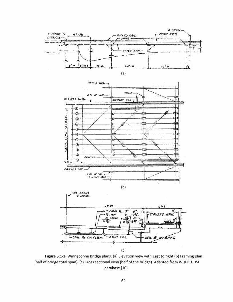
(half o

Figure 5.1‐2

of bridge tota

. Winneconne

al span). (c) C

e Bridge plan

ross sectiona

dat

64

(a)

(b)

(c)

s. (a) Elevatio

l view (half o

tabase [10].

on view with

f the bridge).

East to right

. Adapted fro

(b) Framing p

m WisDOT H

plan

SI

65

Structural Components

The main structural members of the bridge are made of steel. The girders, floor beams,

stringers, and bracing are all components made of grade 36 steel. A summary of the main steel

structural members obtained from WisDOT design drawings [10] can be seen in Table 5.1‐1.

The plate girders on the Winneconne Bridge were built up from angles and flange or cover

plates riveted together to the web plate. To avoid local web buckling, vertical stiffeners (typically double

angles, 2L 3½ x 5 x 5∕16) are provided approximately every 3.6 ft. along the girders as shown in the photo

of Figure 5.1‐3. Furthermore, additional cover plates typically 14 in. by 0.5 in. are bolted on top of the

flanges in required zones. These plate girders have a variable section throughout their span, varying

depth and thickness. The girder’s depth varies from 48 in. at floor beam No. 3 to 126 in. at floor beam

No. 1 (with 1 being closest to the pier).

Floor beams and stringers are common W‐shape sections with constant section along their axis.

Floor beams are connected to the plate girder by rivets (web area) and stub brackets (bottom flange).

The stringers are not continuous between floor beam 1 and 3, being broken at stringer‐floor beam

connections. Their bottom flange is connected to the floor beam flanges by rivets.

Lateral bracing is provided by a V‐shape bracing formed by structural angles along the bridge

axis. Top lateral and bottom bracing are connected to the girders by rivets, both used to prevent lateral

torsional buckling of the girders.

Table 5.1‐1. Main structural elements description and dimensions.


Girder Plate girder with parabolic shape Variable Section

Floor beams Simple span W‐shapes from cl to cl of

girders, spaced at 14ft‐9in

W30x108 (F.B. No. 2 & 3)

Stringers Simple spans W‐shape framed on top of

the floor beams, spaced at 28.5in. W12x28

Top Lateral

bracing

V pattern structural angles connecting the

two girders

L 3½ x 3½ x 5∕16

L 4 x 3½ x 3∕8

L 3½ x 3 x 3∕8

Side Walk C‐shape channels connected to top of the

bascule girder

12 C 30

15 C 33.9

Counter‐Weight

trusses

Combination of Tee sections and double

angles supporting the concrete counter‐

weight

ST 4 WF 24

ST 5 WF 16.5

ST 6 WF 39

2L 7 x 4 x 5∕8

2L 8 x 8 x 3∕4

2L 4 x 3½ x 3∕8

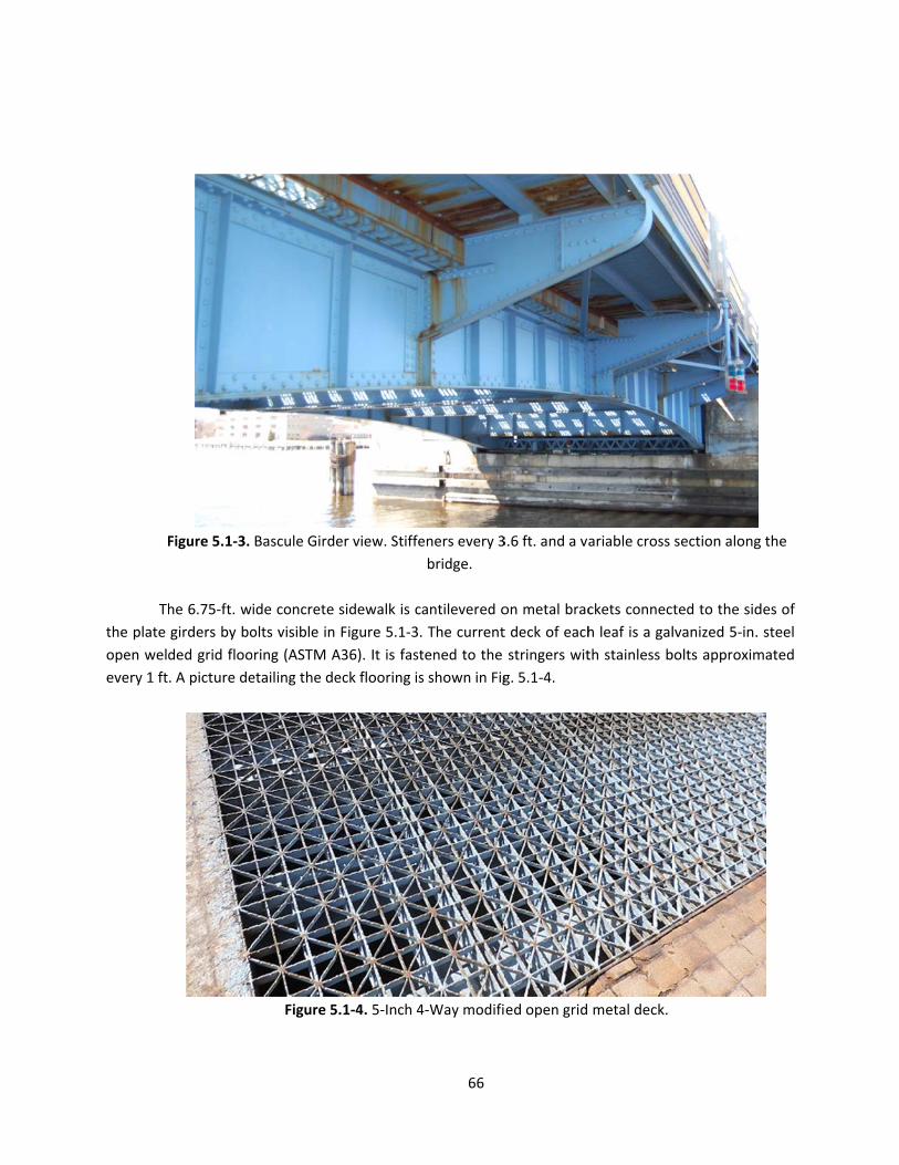
F

Th

the plate

open wel

every 1 ft

Figure 5.1‐3.

he 6.75‐ft. w

girders by bo

ded grid floo

. A picture de

Bascule Girde

ide concrete

olts visible in

oring (ASTM A

etailing the de

Figure 5

er view. Stiffe

sidewalk is c

Figure 5.1‐3.

A36). It is fast

eck flooring is

5.1‐4. 5‐Inch 4

66

eners every 3

bridge.

cantilevered o

. The current

tened to the

s shown in Fig

4‐Way modifi

3.6 ft. and a va

on metal brac

t deck of each

stringers wit

g. 5.1‐4.

ed open grid

ariable cross

ckets connec

h leaf is a gal

th stainless b

metal deck.

section along

ted to the sid

lvanized 5‐in.

bolts approxim

g the

des of

. steel

mated

67

5.2 Winneconne: Development of Three Dimensional Finite Element Model.

Unlike the Mirror Lake and Marinette bridges, the Winneconne bascule bridge was not field

tested. Therefore, the 3D FEM was created according to design plans, visual observations during an

annual bridge inspection, and the experience obtained from the previous Marinette bascule bridge

analysis process. The 3D FEM model of the bridge was created using the commercial CSiBridge software.

OSOW loads were applied to the analytic model to evaluate the bridge performance. Then, critical

members with high stress to capacity ratios were identified. Those will be recommended as the

members to consider in the issuing of permits for future OSOW vehicles.

Model Development

The same types of elements used to model the Marinette Bridge were used in the Winneconne

model. Floor beams, stringers, bracing elements and stiffeners, angles and flanges of the two girder

sections were modeled using frame elements. The steel open grid deck, girder web and counterweight

concrete area were modeled using shell elements. Connections were simulated by links with different

directional stiffness since members like stringers and floor beams had their centroids at different

locations. The links connected the centroid of a stringer, over the floor beam, to the centroid of the floor

beam to resemble the actual geometry as accurately as possible. Bridge geometry was taken from

WisDOT design and shop drawings [10].

In the model, the steel deck to stringer, stringer to floor beam and floor beam to girder

connections were assumed to transfer only shear, no moment. The first two connections were modeled

by using partially fixed linear links, rigidly linking displacement in the vertical direction. These links were

defined from the centroid of each member. In the case of the floor beam to girder connection, a link

element wasn’t necessary since the floor beam ends (frame element) and the girder web (shell element)

shared the same nodes. However, in order to obtain a shear‐transfer connection, end releases were

used at both ends of the floor beam element. Since the floor beams were connected to the girders

through web bolts and stub brackets on the floor beam bottom flange, the actual connection may

transfer shear and some moment. Here the connection was assumed to just transfer shear, and the

effect of the stub bracket was ignored.

The bridge’s mid‐joint connection was assumed to only allow the transfer of vertical shear

forces between the two leaves. The connection was modeled using partially fixed linear links

transferring zero moment between leaves but fully transferring displacements. For this bridge two

model analyses were conducted. In the first one, a tight mid‐joint connection was modeled with a

partially fixed linear link. In the second one, a gap of 0.125 inches at the mid‐joint connection was

modeled with a hook element to see the effects of having a gap in term of stresses in the structure.

Typically

gaps in be

Th

the same

stiffness v

by sharin

together s

Jo

connectio

only rotat

point bet

contact b

like in the

of the mo

Th

cantilever

the joint is a

earings do gro

he counterwe

way as for

values with th

g the same

so the counte

oint restraints

on between t

te about the

ween the “t

etween the t

e Marinette B

odel can be se

he sidewalk w

r, with small

adjusted at le

ow again.

eight, a large

the Marinett

he concrete s

nodes. Again

erweight acte

s used in the

he bascule gi

transverse a

read” and “t

tail beam and

Bridge, this as

een in Figure

Figur

was assumed

stringers, wa

east once per

concrete blo

te bridge mo

shell areas co

n, the “Rigid

ed as a unit.

Marinette Br

irder and the

axis of the br

track” (see Fi

d the approac

ssumption pre

5.2‐1.

re 5.2‐1. (a) Ex

to act as a c

as assumed t

68

r year to elim

ock with embe

odel. Its rigid

nnected rigid

Body constr

ridge model w

e pier was mo

ridge. Vertica

igure 4.1‐1) w

ch span beam

eventing only

(a)

(b)

xtruded mod

cantilever on

to resist none

minate gaps,

edded steel t

behavior wa

dly to the trus

raint” tool w

were also app

odeled assum

al and horizo

was assumed

m was modele

y vertical mov

el. (b) Analyt

the main gird

e of the truc

but with rep

truss member

as modeled b

ss elements a

was used to

plied to the ba

ming that the

ontal moveme

d to be zero

ed by using a

vement at th

tic model.

der as seen in

ck loading bu

peated loadin

rs, was mode

by using very

and the girde

link all the n

ascule girders

bascule girde

ent at the co

(i.e. pinned)

a roller conne

at point. Diag

n Figure 5.2‐2

ut to only cre

ng the

eled in

y high

r web

nodes

s. The

er can

ontact

). The

ection

grams

2. The

eate a

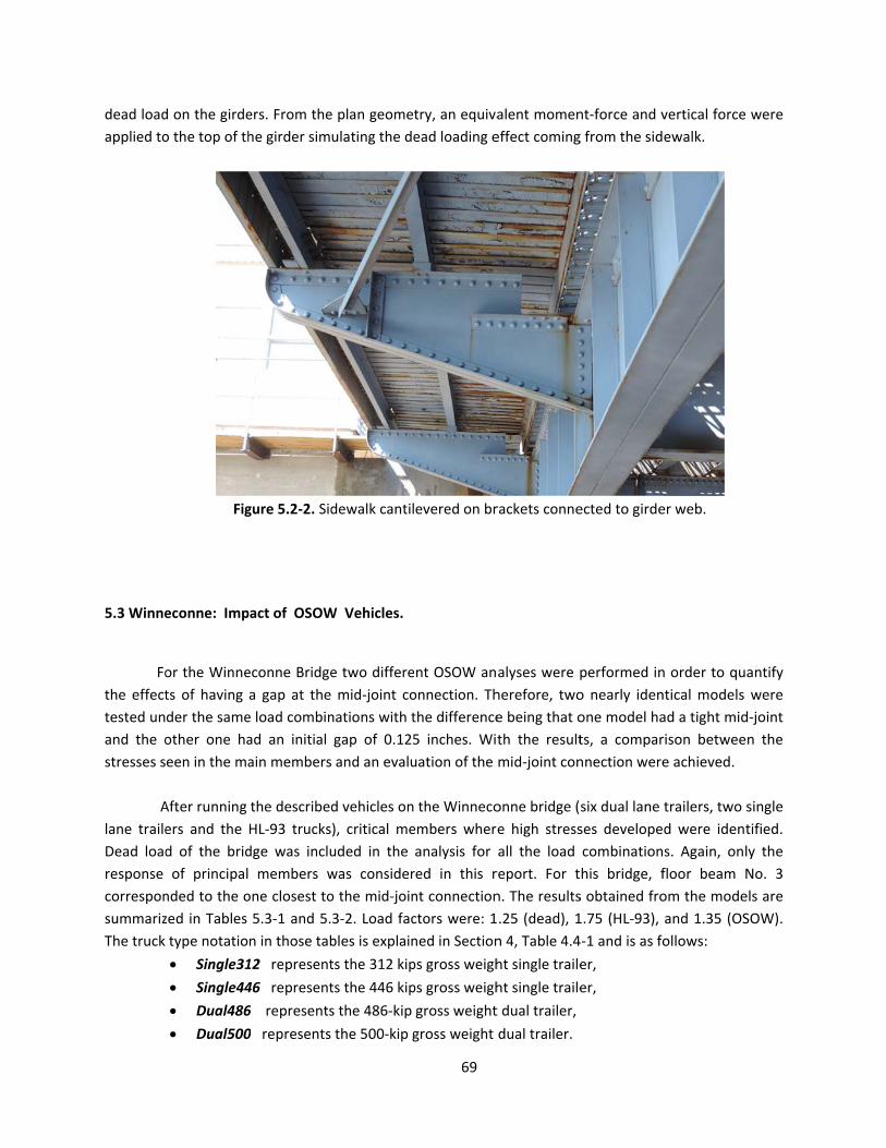
dead load

applied to

5.3 Winne

Fo

the effect

tested un

and the o

stresses s

A

lane traile

Dead load

response

correspon

summariz

The truck

d on the girde

o the top of th

Fig

econne: Imp

or the Winne

ts of having

der the same

other one ha

een in the ma

After running

ers and the

d of the brid

of principal

nded to the o

zed in Tables

type notatio

Single31

Single44

Dual486

Dual500

ers. From the

he girder sim

gure 5.2‐2. Sid

pact of OSOW

econne Bridge

a gap at the

e load combin

ad an initial

ain members

the described

HL‐93 trucks

dge was inclu

members w

one closest to

5.3‐1 and 5.

n in those tab

12 represent

46 represent

6 represents

0 represents

e plan geomet

ulating the de

dewalk cantil

W Vehicles.

e two differe

mid‐joint co

nations with t

gap of 0.125

and an evalu

d vehicles on

), critical me

uded in the

was consider

o the mid‐join

3‐2. Load fac

bles is explain

ts the 312 kip

ts the 446 kip

s the 486‐kip

the 500‐kip g

69

try, an equiva

ead loading e

evered on br

nt OSOW an

onnection. Th

the difference

5 inches. Wit

uation of the

the Winneco

embers where

analysis for

red in this r

nt connection

ctors were: 1

ned in Section

ps gross weigh

ps gross weigh

gross weight

gross weight

alent momen

effect coming

rackets conne

alyses were p

herefore, two

e being that o

th the result

mid‐joint con

onne bridge (

e high stress

all the load

report. For t

n. The results

.25 (dead), 1

n 4, Table 4.4

ht single traile

ht single traile

t dual trailer,

dual trailer.

nt‐force and v

g from the sid

ected to girde

performed in

o nearly iden

one model ha

ts, a compar

nnection were

six dual lane

ses develope

combination

his bridge, f

s obtained fro

1.75 (HL‐93),

4‐1 and is as fo

er,

er,

vertical force

ewalk.

er web.

n order to qu

ntical models

ad a tight mid

rison betwee

e achieved.

trailers, two

d were ident

s. Again, onl

floor beam N

om the mode

and 1.35 (OS

ollows:

were

antify

were

d‐joint

n the

single

tified.

ly the

No. 3

els are

SOW).

M

mid‐joint

Flanges o

while the

deformat

W

5.3‐2 wer

with an i

numbers

loaded st

span adja

Moment enve

are shown in

of the girders

e bottom one

ion and stres

Figure 5.3‐1.

Figure 5.3‐2

With the axial

re developed

nitial 0.125 i

relate to the

ringer, eleme

cent to the m

elopes for diff

n Figure 5.3‐

carry mostly

es are in co

ses adjacent

. Moment env

2. Axial force e

and bending

. The first on

in. gap. Onl

e analytic mo

ent 19, is the

midspan joint.

ferent memb

1. Figure 5.3

y axial force

mpression. T

to the block a

velope on crit

envelope on g

g moment di

ne results fro

y results for

odel element

e 4th stringer

.

70

bers under th

‐2 plots the

in resisting g

The counterw

are insignifica

tical member

girder flanges

iagrams unde

om a model w

the membe

numbering (

in from the g

he moving lo

axial force e

girder mome

weight of the

ant.

rs under OSO

s under OSOW

er each load

with a closed

rs with high

(diagrammed

girder and be

ad combinat

nvelope for t

nts. Top flan

e bridge is s

W/HL‐93 truc

W/HL‐93 truc

combination

mid‐joint an

stress are li

d in the Appe

etween floor

ions with a c

the girder fla

ges are in te

o stiff that g

ck combinatio

ck combinatio

, Tables 5.3‐

nd the second

isted. The str

endix). The hi

beams 2 & 3

closed

anges.

ension

girder

ons.

ons.

1 and

d one

ringer

ighest

3, the

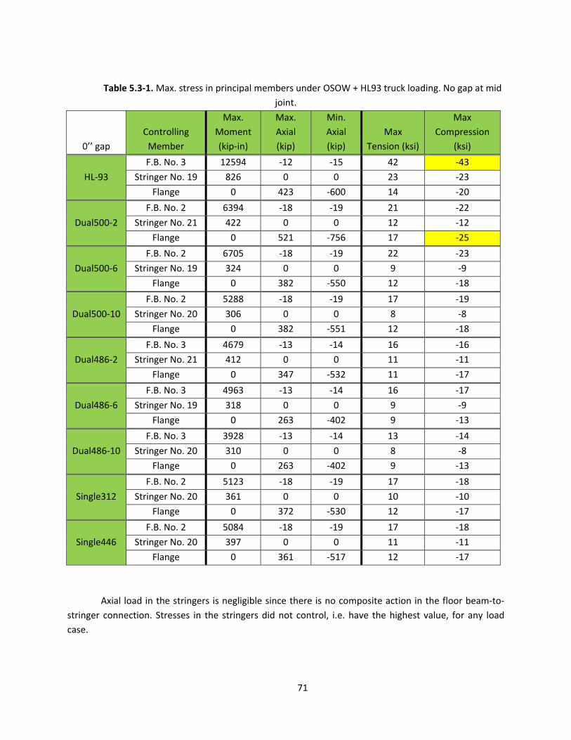
71

Table 5.3‐1. Max. stress in principal members under OSOW + HL93 truck loading. No gap at mid

joint.

0’’ gap

Controlling

Member

Max.

Moment

(kip‐in)

Max.

Axial

(kip)

Min.

Axial

(kip)

Max

Tension (ksi)

Max

Compression

(ksi)

HL‐93

F.B. No. 3 12594 ‐12 ‐15 42 ‐43

Stringer No. 19 826 0 0 23 ‐23

Flange 0 423 ‐600 14 ‐20

Dual500‐2

F.B. No. 2 6394 ‐18 ‐19 21 ‐22

Stringer No. 21 422 0 0 12 ‐12

Flange 0 521 ‐756 17 ‐25

Dual500‐6

F.B. No. 2 6705 ‐18 ‐19 22 ‐23

Stringer No. 19 324 0 0 9 ‐9

Flange 0 382 ‐550 12 ‐18

Dual500‐10

F.B. No. 2 5288 ‐18 ‐19 17 ‐19

Stringer No. 20 306 0 0 8 ‐8

Flange 0 382 ‐551 12 ‐18

Dual486‐2

F.B. No. 3 4679 ‐13 ‐14 16 ‐16

Stringer No. 21 412 0 0 11 ‐11

Flange 0 347 ‐532 11 ‐17

Dual486‐6

F.B. No. 3 4963 ‐13 ‐14 16 ‐17

Stringer No. 19 318 0 0 9 ‐9

Flange 0 263 ‐402 9 ‐13

Dual486‐10

F.B. No. 3 3928 ‐13 ‐14 13 ‐14

Stringer No. 20 310 0 0 8 ‐8

Flange 0 263 ‐402 9 ‐13

Single312

F.B. No. 2 5123 ‐18 ‐19 17 ‐18

Stringer No. 20 361 0 0 10 ‐10

Flange 0 372 ‐530 12 ‐17

Single446

F.B. No. 2 5084 ‐18 ‐19 17 ‐18

Stringer No. 20 397 0 0 11 ‐11

Flange 0 361 ‐517 12 ‐17

Axial load in the stringers is negligible since there is no composite action in the floor beam‐to‐

stringer connection. Stresses in the stringers did not control, i.e. have the highest value, for any load

case.

72

Floor beams developed the maximum stresses identified in any member under the truck

combinations and should be considered the critical bridge member. Different truck combinations

generated maximum stresses in different floor beams. The values for maximum stresses shown above

represent the maximum value found among all the floor beams under a specific load combination. For

example, load combinations HL‐93, Dual486‐2, 486‐6 and 486‐10 induced maximum stresses in floor

beam No. 3 (beam nearest midpan joint), whereas load combinations Single312, Single446, Dual500‐2,

500‐6 and 500‐10 induced maximum stresses in floor beam No. 2.

The maximum stress seen in the floor beams among all the truck combinations was

under the HL‐93 load combination reaching a value of 43 ksi in compression, causing yielding. Dual500‐6

and Dual500‐2 followed with stresses close to 23 ksi, a 47% decrease with respect to the stresses under

the HL‐93 truck. Dual500‐10, Dual486‐6, Single312 & 446 all showed a percentage of smaller of around

60% compare to the HL‐93. Finally, Dual486‐10 is the truck combination that created the lowest stress

among all the trucks on the floor beams, with a 69% decrease with respect to the HL‐93 value.

Again, the maximum overall stress occurred in a floor beam under the HL‐93 truck combination

and was not affected by the gap at midspan. Load combinations HL‐93, Dual486‐2, 486‐6 and 486‐10

induced maximum stresses in floor beam No. 3. Load combinations Single312, Single446, Dual500‐2,

500‐6 and 500‐10 create maximum stresses in floor beam No. 2.

The HL‐93 load combination induced the largest stress reaching a value of 43 ksi in compression,

again causing yielding. Dual500‐6 and 500‐2 loadings followed with stresses close to 23 ksi, a 48%

decrease with respect to the stress under the HL‐93 truck. Dual500‐10, Dual486‐6, Single312 and

Single446 showed a percentage of decrease around 61%. Finally, Dual486‐10 was the truck combination

that created the lowest beam stress among all investigated load cases, with a 69% decrease with respect

to the HL‐93 value. As shown here, the percentage of differences in floor beam stress stays the same

when we have a gap.

The maximum girder flange stress increased by 1 ksi with the open initial gap, to 26ksi with the

Dual500‐2 loading. And from 25ksi to 26ksi when a initially open gap existed at the midspan joint, versus

a tight joint. The gap allows the loaded leaf to deform and resist a portion of the load before the gap

closes. Once the gap closes the adjacent leaf starts to pick up load, but loaded leaf already is carrying an

initial part of the load independently.

Stringer stresses remained low and the open gap had little effect. The stringer stresses remained

at 12ksi or lower under any of the truck loads.

73

Table 5.3‐2. Max. stress in principal members under OSOW + HL93 truck loading.

Gap at mid joint of 0.125’’.

1/8’’ gap

Controlling

Member

Max.

Moment

(kip‐in)

Max.

Axial

(kip)

Min.

Axial

(kip)

Max

Tension (ksi)

Max

Compression

(ksi)

HL‐93

F.B. No. 3 12488 ‐11 ‐15 42 ‐43

Stringer No. 19 820 0 0 22 ‐22

Flange 0 602 ‐708 20 ‐23

Dual500‐2

F.B. No. 2 6408 ‐18 ‐20 21 ‐22

Stringer No. 21 412 0 0 11 ‐11

Flange 0 600 ‐795 20 ‐26

Dual500‐6

F.B. No. 2 6718 ‐18 ‐20 22 ‐23

Stringer No. 19 318 0 0 9 ‐9

Flange 0 436 ‐575 14 ‐19

Dual500‐10

F.B. No. 2 5303 ‐18 ‐20 17 ‐19

Stringer No. 20 300 0 0 8 ‐8

Flange 0 437 ‐575 14 ‐19

Dual486‐2

F.B. No. 3 4641 ‐12 ‐14 15 ‐16

Stringer No. 21 406 0 0 11 ‐11

Flange 0 437 ‐582 14 ‐19

Dual486‐6

F.B. No. 3 4915 ‐12 ‐14 16 ‐17

Stringer No. 19 315 0 0 9 ‐9

Flange 0 327 ‐434 11 ‐14

Dual486‐10

F.B. No. 3 3890 ‐12 ‐14 13 ‐14

Stringer No. 20 306 0 0 8 ‐8

Flange 0 326 ‐434 11 ‐14

Single312

F.B. No. 2 5149 ‐18 ‐20 17 ‐18

Stringer No. 20 356 0 0 10 ‐10

Flange 0 464 ‐581 15 ‐19

Single446

F.B. No. 2 5144 ‐18 ‐20 17 ‐18

Stringer No. 20 391 0 0 11 ‐11

Flange 0 464 ‐562 15 ‐18

Summary of Results for Closed and Open Mid Joint ‐ Winneconne’s 3D FEM

From results seen in Tables 5.3‐1 and 5.3‐2, maximum stresses occurred in the floor beams

under the HL‐93 truck combination, reaching values past yield of 43 ksi, regardless of whether there is

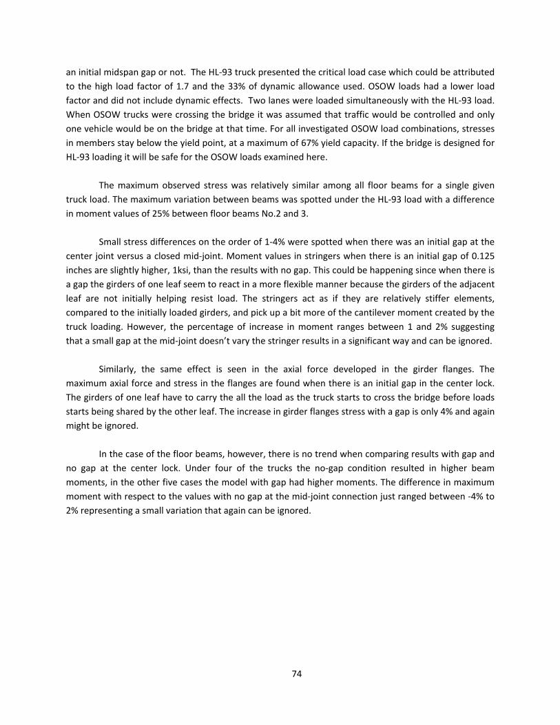
74

an initial midspan gap or not. The HL‐93 truck presented the critical load case which could be attributed

to the high load factor of 1.7 and the 33% of dynamic allowance used. OSOW loads had a lower load

factor and did not include dynamic effects. Two lanes were loaded simultaneously with the HL‐93 load.

When OSOW trucks were crossing the bridge it was assumed that traffic would be controlled and only

one vehicle would be on the bridge at that time. For all investigated OSOW load combinations, stresses

in members stay below the yield point, at a maximum of 67% yield capacity. If the bridge is designed for

HL‐93 loading it will be safe for the OSOW loads examined here.

The maximum observed stress was relatively similar among all floor beams for a single given

truck load. The maximum variation between beams was spotted under the HL‐93 load with a difference

in moment values of 25% between floor beams No.2 and 3.

Small stress differences on the order of 1‐4% were spotted when there was an initial gap at the

center joint versus a closed mid‐joint. Moment values in stringers when there is an initial gap of 0.125

inches are slightly higher, 1ksi, than the results with no gap. This could be happening since when there is

a gap the girders of one leaf seem to react in a more flexible manner because the girders of the adjacent

leaf are not initially helping resist load. The stringers act as if they are relatively stiffer elements,

compared to the initially loaded girders, and pick up a bit more of the cantilever moment created by the

truck loading. However, the percentage of increase in moment ranges between 1 and 2% suggesting

that a small gap at the mid‐joint doesn’t vary the stringer results in a significant way and can be ignored.

Similarly, the same effect is seen in the axial force developed in the girder flanges. The

maximum axial force and stress in the flanges are found when there is an initial gap in the center lock.

The girders of one leaf have to carry the all the load as the truck starts to cross the bridge before loads

starts being shared by the other leaf. The increase in girder flanges stress with a gap is only 4% and again

might be ignored.

In the case of the floor beams, however, there is no trend when comparing results with gap and

no gap at the center lock. Under four of the trucks the no‐gap condition resulted in higher beam

moments, in the other five cases the model with gap had higher moments. The difference in maximum

moment with respect to the values with no gap at the mid‐joint connection just ranged between ‐4% to

2% representing a small variation that again can be ignored.

6.1 Came

Th

the Missis

truss prov

bridge is

arches, on

rib at the

system. T

stringers

Vertical h

aid in resi

twenty‐on

50 ft. and

south side

ron Avenue:

he Cameron A

ssippi River i

vide for easte

an x‐braced s

ne on each si

e bottoms. T

The superstru

which in tur

angers, conn

isting vertical

ne transverse

d consists of t

e (Figure 6.1‐

6.

Introductio

Ave arch brid

n the city of

erly traffic an

steel tied‐arc

de of the roa

he tie resists

cture system

n are suppor

necting the ar

l loading. The

e floor beams

two vehicle la

2).

CAMERON

n and Structu

dge (B‐32‐202

La Crosse, W

nd westerly tr

ch bridge wit

adway, acting

s horizontal t

m is composed

rted by trans

rch ribs and t

e total span o

s along with t

anes of 15 ft.

Figure 6.1‐1.

75

NAVENUE

ural Compon

2), built in 200

Wisconsin. Co

raffic respect

h vertical do

g together wit

thrust from t

d of a partial

sverse floor b

the tie girders

f the arch bri

the two main

and 18 ft. re

Cameron Av

EBRIDGE

ents

04, is one of

mbined, the

ively across t

uble hangers

th tie girders

the arches a

composite c

beams that c

s, were place

idge is 475 ft

n tie girders. T

spectively an

ve Bridge

the two long

Cameron arc

the river. The

s. The tied‐ar

s rigidly conne

nd partially s

concrete deck

connect into

ed at every ot

. with six long

The width be

nd an 8 ft. wid

g span bridges

ch and the C

e Cameron Av

rch bridge ha

ected to each

supports the

k over longitu

the main gi

ther floor bea

gitudinal strin

etween arch

de sidewalk o

s over

ass St

venue

s two

h arch

e deck

udinal

rders.

am to

ngers,

ribs is

on the

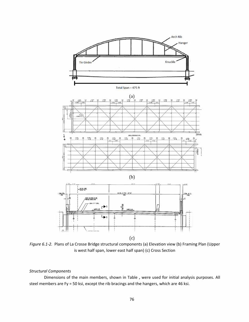
Figure 6.1

Structural

D

steel mem

1‐2. Plans of

l Components

imensions of

mbers are Fy =

La Crosse Brid

is west hal

s

f the main m

= 50 ksi, exce

dge structura

f span, lower

embers, show

ept the rib bra

76

(a)

(b)

(c)al component

r east half spa

wn in Table ,

acings and the

ts (a) Elevatio

an) (c) Cross S

, were used f

e hangers, wh

on view (b) Fra

Section

for initial ana

hich are 46 ks

aming Plan (U

alysis purpose

si.

Upper

es. All

77

Table 6.1‐1. Main Component dimensions

Member

Name Type Dimension

Tie1 Main bolted box section with angles

69×30×1.5×0.75

(depth × width × flange thickness × web

thickness)

Tie2 Heavier equivalent tie girder section used at

the tie/arch knuckle

69×30×1.5×1.375


thickness)

Arch1 Main arch rib welded box section

69×31.2×1.375×1.375


thickness)

Floor beams Simple span I‐beam from cl to cl of tie girders

Cross section depth varies from 4.58ft

to 5.2ft

(DetailsseeFig. 6.1‐3)

Stringers Simple spans framed into the floor beams W 24×55

Arch bracing X pattern using structural tubing TS 20×12×1/2

Lower

Lateral X pattern connecting at the hanger locations W 12×58

Hangers A set of bridge strands at each hanger

location Diameter 2‐3/8in.

The tie girders consist of box sections with internal stiffener diaphragms (see Figure 6.1‐3a)

every 22.5 ft. These box sections are composed of webs and flange plates bolted together using angles.

Spreadsheets were used to compute properties of equivalent HSS sections. In Table , Tie 1 is the tie

section used for most of the length while Tie 2 is a section with heavier webs that represents the

arch/tie knuckle joint. Bending stiffness of the tie girder is very important in a system such as the one

used on this bridge, where only every other floor beam has a hanger, to distribute superstructure live

loads evenly to the arch.

The arches, unlike the tie girders, are welded box sections. While the arches would preferably

resist primarily axial compressive force, bending is also of concern particularly when the bridge is loaded

with asymmetric concentrated loading. The arch shape is efficient for uniform loading, but asymmetric

loading will introduce uneven tension forces in different hanger locations and create bending in the

arch. X pattern rib bracing between the arches provides buckling stability to the arches when under

compressive force.

Two bridge strands of 2‐3/8in. diameter each are used to form a tension hanger set that

suspends the tie girders from the arches at each tie location (Figure 6.1‐3a). The two strands are spaced

16 inches apart and parallel to the bridge span, providing a total hanger area of 6.76 square inches. Each

set of strands are held firmly into two grooved open strand sockets, which are rigidly bolted into the

diaphragm

outside th

Figure 6.

co

Fl

varied we

and flange

H

the floor

beams. T

stringer t

ms of both th

he openings w

1‐3. Non‐pris

nnection (ele

loor beams a

eb depth acro

es are bolted

eight conside

beam flange

herefore the

to be bolted

he arch and gi

where the str

(a)

smatic floor b

evation view)

are non‐prism

oss the width

into the tie g

erations led t

s. Rather tha

top flange w

into the sti

irder section

ands extend

beam configur

(b) Cross sec

matic I‐beams

of the bridge

girder with an

to placement

an being supp

was coped an

iffener of th

78

via thick guss

into the flang

(c)

rations and co

tion through

s with uniform

e to provide c

ngle plates as

t of the string

ported on the

nd the bottom

e floor beam

set plates. Se

ges of the box

(b)

onnection de

floor beam (

m web thickn

crown in the r

shown in Fig

gers with the

e floor beam

m flange was

m as detaile

eals are clamp

x sections.

etails: (a)Floo

c) Floor beam

ness and flan

roadway surfa

gure 6.1‐3a&b

eir top flange

ms, the stringe

s cut on one

d in Figure

ped to each s

r beam and g

m elevation.

nge dimensio

ace. Both the

b.

es at the heig

ers frame int

e side to allow

6.1‐4. Deck

strand

girder

on but

e web

ght of

to the

w the

shear

connecto

towards t

Th

transverse

33ft. road

stringers a

connectio

deck. Stu

rested on

rs are spaced

he center to

he concrete d

ely and longi

dway and an

and the floor

ons (studs) p

ds were not

the floor bea

(a) String

Figu

d on the strin

provide comp

deck is cast‐in

tudinally thro

8ft. wide sid

r beams abou

rovided, full

provided bet

ams.

ger dimension

(b) String

ure 6.1‐4. Stri

nger top flang

posite action

n‐place with u

ough the slab

dewalk only

ut 1.25 in. and

composite a

tween the de

n and shear c

ger and floor

inger shear st

79

ge at 6in. apa

with the con

uniform dept

b. The total w

on the south

d 5.875 in. res

ction could b

eck and floor

connection (s

beam conne

tuds and floo

art near the e

ncrete deck.

th of 8 in. wit

width of the

hern side. Th

spectively. As

be achieved

r beam, altho

studs) spacing

ection (plan v

r beam conne

ends and incr

h reinforcing

deck is 44ft.

e deck is ha

s mentioned

between the

ough haunche

g (elevation v

view)

ection details

rease to 8in.

steel intersp

. and consist

unched abov

before, with

e stringer an

es below the

view)

s

apart

persed

s of a

ve the

shear

nd the

e deck

6.2 Came

Th

three, onl

of this bri

checking t

Selection

A

maximum

loading ca

maximum

prelimina

maximum

that conn

measured

Accuratel

that wou

measure s

the

we

as

we

eron Avenue:

hree large‐sc

ly the Camero

dge location,

the accuracy

of Test Locat

lthough max

m bending in t

ases. Before

m strain effec

ry analyses p

m strain. This s

nects to the ti

d in the floor

y measuring

ld likely hav

strain. The fo

e second pair

eb of the fifth

the hanger H

eb of the two

: Field Load T

ale tied arch

on Ave bridge

, i.e. over the

of predicted

ion

ximum axial

the arch and t

the field load

cts in certain

predicted that

strain would

ie girder at th

beam, the ha

very low leve

ve the larges

ollowing locat

r of hangers (

h floor beam

H2,

tie girder sec

Testing

bridges were

e was chosen

Mississippi r

internal com

force in the

tie girders oc

d test was co

bridge elem

t the second

occur with st

hat hanger lo

angers and th

els of strain in

st strain valu

ions were ins

H2) from the

(FB5) from t

ctions (T3 and

80

e selected for

n for field test

river. Field tes

ponent force

e arch is gen

ccurs with just

onducted, pos

ents were an

set of hanger

tationary truc

cation. Using

e tie girder se

n structural m

ues would be

strumented (F

west end on

he west end

d T4) that we

r examination

ting due to th

st results are

es from initial

nerated whe

t part of the s

ssible locatio

nalyzed using

rs, from the a

ck wheel load

g that positio

ection near t

members is di

e the best t

Figure 6.2‐1):

the south sid

that connect

re just west o

n as part of th

he critical rero

intended to

software ana

en the whole

span is loade

ons of truck lo

g an initial an

arch end, wou

ding right abo

n of truck loa

he hanger/flo

ifficult in the

targets for in

:

de of the brid

ts into the sa

of the H2 han

his study. Of

outing‐impor

provide a bas

alyses.

e span is lo

ed, i.e., asymm

oad placeme

nalytic mode

uld experienc

ove the floor

ading, strains

oor beam loc

field, so mem

nstrumentatio

dge,

me girder loc

nger location.

those

rtance

sis for

oaded,

metric

nt for

l. The

ce the

beam

were

ation.

mbers

on to

cation

Figure 6.

Loading R

Tw

bridge ins

axles sepa

Th

hangers.

south edg

above the

truck drov

as possibl

outer whe

position.

analytic m

2‐1. Instrume

tie girder

Regime

wo dump tru

spection, wer

arately) befor

he load regi

First two dum

ge of the dec

e 5th floor be

ve backwards

le to the dum

eels to the ba

Locations of

modeling. Tru

entation locat

sections (b) g

ucks of know

re used to im

re arriving at

me was des

mp trucks he

ck (wheels ad

eam (which c

s along the so

mp truck adja

arrier foot an

each wheel

ck locations a

tions: (a) elev

gage location

wn weight an

pose stationa

the bridge fo

igned to ach

eading east w

djacent to th

onnects to th

outh edge (ca

cent to the b

nd that betwe

load relative

are shown in

81

vation view (S

ns on No.5 flo

d dimension

ary live loadin

or testing.

hieve a high

were parked s

e barrier) wi

he instrumen

b headed we

barrier as sho

een each whe

to the tie gi

Figure 6.2‐2b

(a)

South) with g

oor beam (Sou

s, along with

ng. Each truc

strain in the

side by side a

ith the cente

nted second

est) and parke

wn in Figure

eel were mea

irder center w

b.

age locations

uth is to the r

h the UB‐60

ck was weighe

e instrument

and as close

er of their ba

hanger set).

ed with its rea

6.2‐2a. The d

asured when

were calculat

s on H2 and T

right).

snooper truc

ed (front and

ted second s

as possible t

ack two axles

Then the sno

ar bumper as

distances from

the trucks w

ted to use la

T3, T4

ck for

d back

set of

to the

s right

ooper

s close

m the

ere in

ater in

Figure 6.2

Gage Inst

Tw

VW gages

measure t

Tw

snooper t

inches up

beam in o

to remove

spot weld

anti‐corro

Tw

Figure 6.2

center, th

on the gir

2‐2. Instrume

relative to

tallation

wo Geokon 4

s with a 1.75

the strain cha

wo foil gages

truck at the

p and down r

order to meas

e paint, the m

ded on the cl

osion spray co

wo short VW

2‐1 using a s

he actual posi

rder web and

entation loca

o south girder

4000 vibrating

5‐in gage len

ange during t

s were appli

location show

respectively f

sure axial and

metal was furt

eaned patche

oating.

W gages and t

similar proced

tions were sl

6.2‐3c&d sho

tions (a) truc

r (bold line re

g wire (VW) g

ngth, and fou

he load test.

ed on the w

wn in Figure

from the cen

d bending stra

ther cleaned

es directly us

two foil gage

dure. Though

ightly varied

ow the VW ga

82

(b)ks (South is t

epresents the

gages with 6‐

ur 0.25‐in lon

web of the fif

6.2‐3a. The

nter of the be

ains. After th

by hand with

sing a Sunsto

es were appl

h the gages w

as shown in

age applicatio

o the right),

e center line o

‐in gage leng

ng weldable

fth floor bea

beam gages

eam, oriente

e location wa

h sandpaper a

one Pulse Tac

ied on the ti

were intende

Figure 6.2‐1.

on.

(b) plan view

of the south g

th, two Geok

foil strain ga

am from the

s were applie

ed parallel to

as sanded wit

and alcohol. T

ck Welder an

ie girder at lo

ed to be 20in

Figure 6.2‐3b

w location of t

girder.

kon 4100 wel

ages were us

west end us

ed on the we

the length o

th electric gri

The gage the

d finished wi

ocations sho

n. from the g

b shows a foi

trucks

ldable

sed to

sing a

eb, 20

of the

nders

n was

ith an

wn in

girder

l gage

Figur

weldable

Th

friction cl

deck leve

re 6.2‐3. Gage

e foil gage use

he Geokon 4

amps on the

l to avoid loca

(a)

(c)

e installation

ed on box gird

4000 VW stra

two hangers

al stress conc

‐ a) applying

der web, c) V

cover

ain gages an

as visible in F

centration ne

83

gages on the

W gage weld

and lead wir

nd vibrating c

Figure 6.2‐4.

ar the hanger

5th floor bea

ed on box gir

e.

coils with wi

Both gages w

r end connec

(b)

(d)

m with a sno

rder web, and

ire leads we

were at appro

tions.

oper truck, b

d d) VW gage

re mounted

oximately 6ft.

b)

with

using

. from

Data Colle

To

the bridge

were driv

the readin

order to r

the bridge

A

the truck

Unfortuna

results.

In

compress

the tie gir

force. It d

two floor

Figu

ection Schem

o start the te

e. An initial r

ven into their

ngs, the exact

repeat the sa

e, another rea

fter the data

s present. Th

ately the VW

nspecting the

sion, is smalle

rder since it re

oesn’t seem

beam strains

ure 6.2‐4. VW

e and Results

est, the City o

eading of all

positions, th

t truck axle lo

me loading in

ading was tak

a was collecte

he resulting

W gages in th

two girder st

er in value tha

esists the hor

reasonable fo

s can be used

W strain gages

s

of La Crosse

the gages wa

he strains und

ocations on th

n the analytic

ken to see if a

ed, the initial

values, the s

e tie girder m

trains and the

an the bottom

rizontal thrus

or the floor b

to define a n

84

with vibratin

police blocke

as taken with

der stationary

he deck edge

cal model late

any drift deve

l gage readin

strains create

malfunctione

e floor beam

m strain, a ten

t from the ar

eam – which

neutral axis. W

ng coils on bri

ed traffic to e

h no vehicles

y truck loadin

and relative

er. Finally afte

eloped in the

ngs were subt

ed by the tru

d but the ne

strains it is cl

nsion. That co

ch and should

should not b

With the high

dge hangers.

eliminate veh

on the bridg

ng were colle

to each othe

er all the truc

gage reading

tracted from

ucks, are list

earby foil gag

ear that ther

ondition wou

d be carrying

be carrying ax

tension strai

.

hicles passing

ge. Then the t

ected. While t

r were record

cks were drive

gs.

the readings

ed in Table

ges provided

re the top stra

uld be expecte

g an axial tens

xial tension. T

in at the bott

g over

trucks

taking

ded in

en off

s with

6.2‐1.

good

ain, a

ed in

sion

The

om

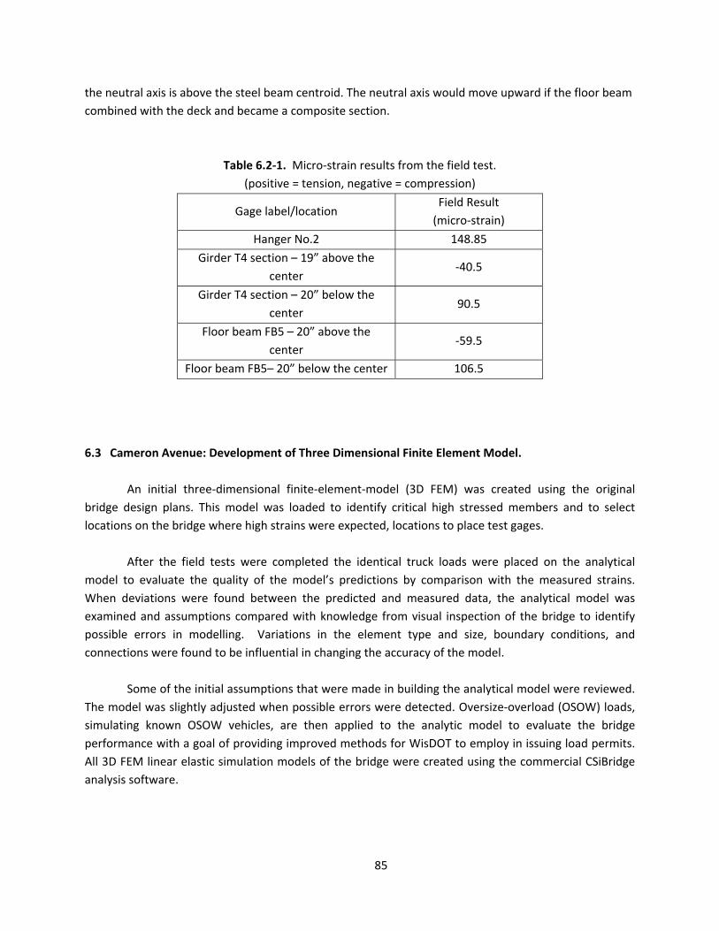
85

the neutral axis is above the steel beam centroid. The neutral axis would move upward if the floor beam

combined with the deck and became a composite section.

Table 6.2‐1. Micro‐strain results from the field test.

(positive = tension, negative = compression)

Gage label/location Field Result

(micro‐strain)

Hanger No.2 148.85

Girder T4 section – 19” above the

center ‐40.5

Girder T4 section – 20” below the

center 90.5

Floor beam FB5 – 20” above the

center ‐59.5

Floor beam FB5– 20” below the center 106.5

6.3 Cameron Avenue: Development of Three Dimensional Finite Element Model.

An initial three‐dimensional finite‐element‐model (3D FEM) was created using the original

bridge design plans. This model was loaded to identify critical high stressed members and to select

locations on the bridge where high strains were expected, locations to place test gages.

After the field tests were completed the identical truck loads were placed on the analytical

model to evaluate the quality of the model’s predictions by comparison with the measured strains.

When deviations were found between the predicted and measured data, the analytical model was

examined and assumptions compared with knowledge from visual inspection of the bridge to identify

possible errors in modelling. Variations in the element type and size, boundary conditions, and

connections were found to be influential in changing the accuracy of the model.

Some of the initial assumptions that were made in building the analytical model were reviewed.

The model was slightly adjusted when possible errors were detected. Oversize‐overload (OSOW) loads,

simulating known OSOW vehicles, are then applied to the analytic model to evaluate the bridge

performance with a goal of providing improved methods for WisDOT to employ in issuing load permits.

All 3D FEM linear elastic simulation models of the bridge were created using the commercial CSiBridge

analysis software.

Initial Mo

U

model wa

A

defined w

calculatio

Therefore

cross‐sect

section a

previous T

are used

represent

rigid conn

girder sta

Si

floor beam

of the brid

6.3‐1, the

decreases

directions

web and t

transfer.

It

though sh

odel Developm

sing the desi

as prepared a

s suggested b

with the exact

n compared

e, the tied gird

tion with the

llowed corre

Table 6.1‐1, T

for most of t

ting the tie gi

nection with

rt and end no

imilarly, the n

ms are broke

dge’s varying

e section dep

s to 4.58ft. a

s of translatio

the flanges o

was assume

hear connecto

ment

gn plans from

s illustrated i

Figure 6.

by Chung et a

t shape can p

to modelling

der and arch

same stiffne

ct modelling

Tie 1 represen

the length of

irder where i

the arch. Th

odes were cal

non‐prismatic

n into three s

section in th

th linearly in

t E9. At the

on and rotatio

f the floor be

ed that comp

ors were not

m the WisDOT

n Figure 6.3‐1

.3‐1. 3D FEM

al. (2005), wh

provide predic

it with differ

were modell

esses as the c

of the tie g

nts the tie gir

f the girder. T

t joins with t

he bridge has

lculated using

c floor beam

segments – e

at segment. T

creases from

ends of the

ons into the t

eam are bolte

osite action d

employed. T

86

T HSI (Highwa

1.

M model of Ca

en modeling

ction of the s

rent shell elem

ed with fram

complex ones

girder with in

rder sections

Tie 2 is a sec

the bottom o

s a vertical c

g spreadshee

s are I‐shape

each having a

The actual lin

4.52ft. to 4.

floor beams,

tie girder wer

ed (Figure 6.1

developed be

The deck is ha

ay Structures

meron Ave B

beam section

same accurac

ments for the

me elements t

s on the bridg

nner diaphrag

(divided leng

ction (25.25 f

of the arch. T

urve and the

ets to model t

ed sections w

a uniform cro

near variation

82ft. along E

, rigid connec

re assumed f

1‐3a&b) to th

etween the f

aunched dow

s Information

Bridge

ns using a sin

cy but with m

e web and fla

that had the p

ge. This use o

gms and cor

gth wise into

ft in length) w

he girder is a

e varying ele

the actual pro

with varying d

ss section eq

n of the sectio

E1 through E4

ctions that tr

for the model

he tie girders,

floor beams a

wn to the top

System), an

gle frame ele

much less ana

anges respect

properties of

of a simulate

ner angles. I

23.5 ft. each

with heavier

assumed to h

vation of ea

ofile.

epth. The mo

qual to the av

on is listed in

4 and then lin

ransfer force

l because bot

, allowing mo

and the deck

of the floor

initial

ement

lytical

tively.

a box

d box

n the

h) that

webs

have a

ch tie

odel’s

verage

Table

nearly

in all

th the

oment

k even

beam

so there

partially c

A

beams. W

from the

are just si

in the stri

connectio

floor beam

Fo

cable elem

the two o

arch and h

Th

floor beam

connectio

detailed i

is likely shea

composite act

Figu

s shown in Fi

While the nor

centerline of

itting on an a

ngers are not

on (Figure6.1‐

ms are model

or simplicity o

ment has a d

original bridge

hanger to tie

he concrete

ms. The slab

ons on the to

n Figure 6.3‐3

ar capacity e

tion. A fully co

ure 6.3‐2. Flo

igures 6.1‐4 a

rmal interval

f the north a

angle which is

t transferred

‐4). In terms

led as hinged

only one cab

iameter of 2

e strands, 6.7

girder are int

deck has a u

and the strin

op flange of

3.

(a)

xisting due t

omposite act

or beam fram

and 6.3‐3, six

between stri

nd south tie

s bolted to a f

into the floo

of the initial

connections

le is used in t

.933in. to pro

76 square inc

terpreted as s

uniform 8‐in.

ngers were co

the stringer

Shearcon

87

to bond and

tion was assu

me element d

longitudinal

ingers is 84in

girders, resp

floor beam w

r beams beca

model, the

transferring

the model to

ovide an iden

ches. Anchora

straight rigid

depth. Haun

onsidered as

spaced at 6

nnection(stu

friction. This

med in the in

definition (Ele

discontinuou

n., Stringer 1

pectively. The

web stiffener.

ause there is

connections

no bending m

o represent a

ntical total cr

age connectio

elements in t

nches are pro

fully compos

6in. near the

uds)spacing

s might best

nitial model.

evation view)

us stringers fr

and Stringer

e lower flang

This implies

no bottom fl

between the

moment into

set of two ha

ross section a

ons between

the model.

ovided above

site with the

e ends and 8

onthestring

be consider

rame into the

r 6 are 65in.

es of the stri

that the mom

ange or top f

e stringers an

the floor bea

angers. The m

area as the su

the hanger t

e the stringer

presence of

8in. in betwe

gers

red as

e floor

away

ingers

ments

flange

nd the

ams.

model

um of

to the

rs and

shear

en as

D

and econ

modeling

sections a

are insert

rather sim

slab‐beam

segment.

Sh

compone

recomme

accounts

However,

each shel

were divid

element c

and 8‐in

connectio

Details of

Element

Name

Tie1

Tie2

ifferent slab‐

nomical meth

method esse

and places sh

ted between

mple, it is pro

m interaction.

In this mode

hell element

nt is governe

nded for an

for transvers

Mindlin shel

l element is

ded according

corners with s

apart elsewh

on between th

the finite ele

t ASTM

Materia

A709

HPS50W

A709

HPS50W

Figure 6.3‐3

‐beam system

hod for this

entially utilize

ell elements

the beam ce

ven to be acc

. The beam m

l the stringer

s are widely

ed by flexure

accurate ana

se shear defo

lls are suscep

further divid

gly, changed

straight vertic

here, a fully‐

he shell elem

ement modell

Table 6.3‐1

al

Elemen

type

W

Box/Tub

Section

W

Box/Tub

Section

(b)Sh

3. Shear conn

m modeling te

bridge. As s

es straight fra

at the centro

entroid and d

curate when

must be sepa

links to the d

used to ide

e. More speci

lysis (compar

ormation, tho

ptible to “shea

ded into appr

from the init

cal links. Give

‐composite a

ments and the

ling are summ

1. Details of

t Cross‐se

be

n

69×

depth × w

fla

be

n 69×3

88

earconnecti

nection provid

echniques we

suggested by

ame elements

oid of the con

deck to ensu

predicting de

rated into sh

deck were init

ealize the bri

ifically, a thic

red to thin sh

ough this may

ar lock” which

roximately 1f

ial 84in. secti

en that studs

action is assu

e stringers wa

marized in Tab

model finite e

ection Dimensi

(inches)

30×1.5×0.75

width × thickn

ange × web

30×1.5×1.375

iondetails

ded on the st

ere reviewed

y Chung et a

s with the geo

ncrete slab. Th

ure composit

eflection, stra

ort segments

tially placed a

dge deck sin

ck shell elem

hell element

y not be sign

h is caused b

ft by 1ft sect

ions, to creat

are 6‐in apar

umed in the

as used to ass

ble 6.3‐1.

element mod

on Segm

ess

tringers.

d in order to

al. (2005) th

ometric prop

hen, vertical

e action. Wh

ain, and flexu

s with links a

at 84in. interv

nce behavior

ment (Mindlin

a.k.a. Kircho

nificant in a b

y large aspec

ions. Then th

e nodes that

rt near the en

initial mode

sure the fully

delling.

ment length

23.5ft

25.25ft

select an acc

he eccentric

erties of the

rigid link elem

hile this meth

ral behavior o

t the ends of

vals

of this stru

type) is gen

ff type) beca

bridge applic

ct ratios. Ther

he stringers b

connect with

nds of the stri

el. A 28in. sp

composite a

Number

elements

18 in one g

2 in one g

curate

beam

beam

ments

hod is

of the

f each

ctural

nerally

use it

ation.

refore

below

h shell

ingers

paced

ction.

r of

used

girder

girder

89

Arch A709

HPS50W

Box/Tube

Section 69×31.2×1.375×1.375

Projected horizontal distance same as

each girder sections

20 in one arch

Floor

Beams

A709

HPS50W

I/Wide

Flange

Section

16×1.5×0.5

flange width × thickness

× web thickness

various section depths

North end to “kink”:

23.1ft

Depth: 4.82ft to 5.2ft

“Kink” to South end:

31.1ft

Depth: 5.2ft to 4.58ft

1 each floor

beam

Stringers A709

HPS50W

I/Wide

Flange

Section

W 24×55 23.5ft

6 longitudinally

partitioned into

20 separated

segments by the

floor beams

Rib

Bracing

500

Grade B

(46 ksi)

Box/Tube

Section TS 20×12×1/2 Approx. 68.6ft

16 used to

brace the two

arches

Lower

Lateral

A709

Grade

HPS50W

I/Wide

Flange

Section

W 12×58 Approx. 68.6ft

20 used to

brace the two

ties and resist

wind loads

Hangers 586 Class C

(100 ksi)

Cable

Section

Diameter 3.588 in

Equivalent to dual strands

Between the hanger

connections

9 between tie

and arch on

same side

Hanger

Connections

A709

Grade

HPS50W

Custom

general

section

High moment and shear

resistance

5ft down from arch

center and 3.5ft up

from tie center

2 for each

hanger

Concrete

Slab

f’c=4000psi

Thick shell 8in thick 23.5ft × 7ft 10in

(length × width)

Total width 44ft

× 475ft

In the analytic model, the connections between different elements and element types are

where oversimplified assumptions could be made and therefore induce modeling errors that could

accumulate and affect the overall accuracy of the model significantly. Link elements are used in joints

and different degrees of freedom are defined according to the real connection cases. Hinged joints only

transfer translations in x‐, y‐ and z‐ translations whereas the rigid joints transfer both translations and

rotations in three directions between the connected elements. The locations of each joint type in this

bridge are shown in Table 6.3‐2.

Table 6.3‐2. Joint modeling details

Joint Location Joint Type

Stringer to floor beam Hinged joint

Floor beam to tie girder Rigid joint

Tie girder to arch Rigid joint

Hanger to Tie girder Hinged joint

90

Appropriate idealizations and simplifications based on engineering judgement were done when

developing the initial finite element model. Assumptions were made regarding the connections and

support condition. Stringers are assumed as pinned‐pinned connections at the ends to the floor beams,

which in turn are rigidly connected with the girders box sections. Splices between girder sections are

ignored. Link elements that only have freedom in vertical and horizontal directions, but are rigid in those

directions, were used to model the interaction between the concrete deck and the stringers it sat on.

Knuckle sections at the arch and girder joint are not modeled with exact details but by simply joining

them with with a rigid connection. Boundary conditions of the superstructure were idealized as simple

roller and pin supports, such that all translations were constrained at one end while only vertical and

transverse translations were constrained at the other end.

Truck loadings on the model simulated the condition shown previously in Figure 6.2‐2. The loads

from the two dump trucks and the UB‐60 snooper, as applied on the FEM model, are listed in Table 6.3‐

3. The x‐y axes origin in the model was taken at the middle of the entire bridge, with x and y in the plan

of the bridge. The truck wheel loads were applied as point loads. The total load on the bridge was 210.2

kips (thousands of lbs.).

Comparison with Field Measurements

Field strain results collected while all three trucks (two dump trucks and the snooper truck)

were on the bridge are compared with strain predictions from the initial analytic model under the same

loading in Table 6.3‐4 with wheel effects applied as point loads at each wheel location in Table 6.3‐3.

91

Table 6.3‐3. Truck wheel loads and coordinate input for the model.

(“DT” refers to dump truck, truck “A” is close to barrier, UB‐60 is the

snooper, N and S refer to north or south wheel line [south is near

barrier], F‐M‐R refer to front – middle – or rear axle.)

Wheel Location‐X (in) Location‐Y (in) Load (kips)

DT‐A

F‐N 1464 ‐47 11.6

F‐S 1464 ‐129.25 11.6

M‐N 1662 ‐47 12.02

M‐S 1662 ‐129.25 12.02

R‐N 1722 ‐47 12.02

R‐S 1722 ‐129.25 12.02

DT‐B

F‐N 1464 105.75 12.5

F‐S 1464 23.5 12.5

M‐N 1662 105.75 11.455

M‐S 1662 23.5 11.455

R‐N 1722 105.75 11.455

R‐S 1722 23.5 11.455

UB‐60

F‐S 2190 ‐129.25 9.15

F‐N 2190 ‐35.25 9.15

M‐S 1992 ‐129.25 12.43

M‐N 1992 ‐35.25 12.43

R‐S 1938 ‐129.25 12.43

R‐N 1938 ‐35.25 12.43

Table 6.3‐4. Micro‐strain result comparison between the field test and the initial FEM

Gage label Field Result

(micro‐strain)

Initial Model Result

(micro‐strain)

Hanger No.2 149 135

Girder T4 section – 19” above

the center ‐41 ‐43

Girder T4 section – 20” below

the center 91 73

Floor beam FB5 – 20” above

the center ‐59 ‐43

Floor beam FB5– 20” below the

center 106 115

92

Adjustment to the Model Based on Closer Examination of Design Details

Though the strains compared in Table 6.3‐4 showed that the model was working quite well,

improvement might be obtained. In construction of the initial model the floor beams were assumed to

be composite with the deck, even though no connectors were specifically provided between the floor

beam and deck. The concrete bond and possible friction forces were thought to be sufficient to create

composite action.

Figure 6.3‐4 shows the strain diagrams consistent with the measured floor beam and girder

strains, if the strain variation was linear. The initial analytic model gives slightly higher tension at the

beam center of gravity than shown by the field measurement. The neutral axis with the model strains is

also higher than the neutral axis with the measured strains. Both of these observations are consistent

with a model cross section that has composite action – since adding the deck to the beam would bring

the neutral axis higher and increase tension strains in the beam. The measured strains indicate that less

composite action is actually occurring in the floor beams. From the neutral axis location for the

measured data, however, some composite action is obviously present since the neutral axis is not at the

centroid of the beam (and no axial force would be expected in the floor beams).

A modification of the initial model was performed to create partially composite behavior

between the concrete deck and the floor beam. It is possible near midspan of the beam, where vertical

and horizontal shear values are lower, that the beam does develop composite action from concrete

bond or friction. At the beam ends the higher shear forces may break the bond, allowing slip, and

eliminating composite action.

Each floor beam element was initially modeled with 9 nodes, E1 through E9 as shown in Figure

6.3‐2. A revised model then released the composite action at both ends of the beam, allowing relative

transverse displacement between the deck and beam. The result of this modification is also shown in

Figure 6.3‐4 with the strain diagram labelled “Modified”. The model simulation of beam strains was

improved, particularly at the beam bottom. Unfortunately this type of modification can only be achieved

if the actual strain condition in the beam is known. A logical approach to the beam modelling would

normally assume no composite action since there were no studs. With no composite action in the

model, the strain diagram for the beam passed through the beam centroid. The actual measured tension

strain at the center of gravity, clear in the Figure, obviously indicated that a non‐composite modelling

assumption did not simulate the actual bridge condition.

Looking further at the field measurement results In Figure 6.3‐4, one could observe that in the

tie girder section the strain at the girder center of gravity is not zero, due to the tension force in the

member created by the arch thrust. The predicted strains from the initial model are smaller than the

field result. This indicates that modeled girder section should be resisting more axial tension force. No

modificat

member o

Figure 6

Th

bridge tes

error in p

strain is 1

under OSO

ions were m

or geometric

6.3‐4. Linear

r

he Cameron A

st load effects

redicted floo

6 in error, OW vehicle lo

made to the

indication th

strain diagra

ight = linear s

Avenue analy

s. Table 6.3‐5

r beam strain

or 480psi. Th

oads.

Table 6.3‐

Gage labe

Hanger No

Girder T4 se

– 19” above

center

Girder T4 se

– 20” below

center

Floor beam F

20” above

center

Floor beam

20” below

center

analytic mod

at the initial m

ams: left = line

strain diagram

ytic model is c

5 shows that t

n is 20 nearhe adjusted m

5. Compariso

el Fiel

(mic

o.2

ction

e the

ction

w the

FB5 –

the

FB5–

the

93

del to impro

modelling wa

ear strain dia

m over the de

considered to

the error in p

r the beam to

model will be u

on of final stra

ld Result

ro‐strain)

149

‐41.

91

‐59

106

ove girder be

as in error.

gram over th

epth of the flo

o be successfu

redicted hang

op, equivalent

used in predi

ains from test

Adjusted Mo

(micro‐s

150

‐57

96

‐‐39

102

ehavior beca

e depth of th

oor beam.

ul in simulatin

ger strains is

t to 600psi in

cting the brid

t load.

odel Result

strain)

0

7

6

9

2

use there w

he tie girder, a

ng the actual

negligible. T

stress. Tie gi

dge response

as no

and

he

rder

94

6.4 Cameron Avenue: Impact of OSOW Vehicles.

Three types of vehicular loads, i.e. AASHTO the standard HL‐93 notional truck loading and two

types of OSOW vehicles, as described in Chapter 2, were employed in the OSOW bridge response

analyses.

The total road width of the Cameron Ave bridge between parapet walls is 33ft. and consists of

two lanes of 16.5ft. each. Based on their dimensions relative to the lane, two single‐trailers and double

trailers with 2ft. and 6ft. spacing at the center are driven along the center of each lane in this bridge

(because of the asymmetry of the floor beams) and the double trailers with 10ft. between are driven

along the middle of the bridge to generate the practical worst case scenario. An LRFD load factor of 1.75

is applied to the HL‐93 truck; the multi‐presence and dynamic factors were included. Under the OSOW

trucks a single lane was loaded, the LRFD 1.35 load factor is applied and no dynamic effects were

included. Notation for the trucks loads is the same as used in the previous bridge analyses and may be

summarized as:



Dual486 represents the 486‐kip gross weight dual trailer,

Dual500 represents the 500‐kip gross weight dual trailer.

Peak forces and stresses induced in critical members, as predicted by the Cameron Ave analytic

model, by the series of OSOW vehicles are listed in Table 6.4‐1. Table 6.4‐2 lists forces in individual

components with the loading that caused the force. The forces shown for beams and stringers include

the bending moment in the beam alone and added axial force from composite action. Since members

have both axial and bending, and peak values of those forces occur at different locations, two values of

peak stress are calculated for each: based on peak moment or on peak axial. All of the values shown

are 2015 AASHTO LRFD Strength 1 or 2 factored results.

95

Table 6.4‐1. Max stress results in each structural group under factored Dead+HL‐93 loading.

(moments are ft*k, forces are kip, stress is ksi, compression is negative)

Girder

Max Moment

6447

Axial Force

1901

Stress (ksi)

29.3

Max Axial Force

2518

Moment @same location

706

Stress

15.4

Arch

Max Moment

6449

Axial Force

‐2339

Stress

‐24.9

Max Axial Force

‐3083


1667

Stress

‐15.7

Floor Beam

Max Moment

2148

Axial Force

119

Stress

18.1

Max Axial Force

547


912

Stress

14.9

Stringer

Max Moment

171

Axial Force

300.8

Stress

36.3

Max Axial Force

484


51.6

Stress

35.1

Hanger Max Axial Tension

348

Stress

39.2

96

Table 6.4‐2. Maximum member stresses from factored Dead+OSOW truck loads.


Girder

Max Moment

7030

Axial Force

2034

Stress

31.8

Load Case:

Dual500‐2

Max Axial Force

2408


540

Stress

14.4

Dual500‐2

Arch

Max Moment

7104

Axial Force

‐2551

Stress

‐27.4 Dual500‐2

Max Axial Force

‐2925


1427

Stress

‐14.5 Dual500‐2

Floor

Beam

Max Moment

1903

Axial Force

97

Stress

16.9 Dual500‐2

Max Axial Force

553


929

Stress

15.1 Dual500‐2

Stringer

Max Moment

154

Axial Force

298

Stress

34.4 Dual500‐2

Max Axial Force

472


50

Stress

34.2 Dual500‐2

Hanger Max Axial Tension

364

Stress

41.0 Dual500‐2

The highest predicted stress under OSOW loading, listed in Table 6.4‐2, occurs in the bridge’s

hanger cable at midspan with a peak of 41ksi in tension, well below the minimum specified yield stress.

Amongst the flexural members the highest stress, 34.2ksi, occurs in the north side stringer 4ft from the

east end of the bridge. The tie girder develops a stress of 31.8ksi in the north girder at 176ft east of the

bridge center. The arch itself developed a compression stress of 27.4ksi in a section just east of the

second from the east end. All of the maximum stresses occurred under the 500kip dual lane OSOW truck

with trailers spaced at 2ft.

The HL‐93 truck max stresses in the stringer and floor were higher than the stress created by any

of the OSOW vehicles by 5%and 24% respectively. In the arch, tie girder and hanger the HL93 stresses

were 4% to 9% lower than OSOW stresses. The single trailer OSOW vehicles did not impact the bridge

members as much as the HL‐93 or Dual500 trucks.

7.1 Chipp

Th

Chippewa

1, with inc

in 2006 s

the north

separated

separated

7.1‐2c. Af

4ft. sidew

possible t

geometry

stiffening

beams an

to each o

girder.

pewa: Introdu

he Chippewa

a River at Cor

clined structu

howed the 5

h side separat

d the 16ft. ea

d by additiona

fter repairs th

walk on the so

traffic. Photo

y. The two ma

the deck sys

nd twenty set

ther at the e

Figure 7.

7. Ch

uction and St

a River Mem

nell, Wiscons

ural tubing as

50.5ft. wide c

ted from a 14

astbound lan

al barriers ne

he deck had a

outh side and

os taken durin

ain steel trus

stem, which

ts of x‐patter

nds where th

.1‐1. Chippew

hippewa R

tructural Com

orial Bridge

sin. The struct

s diagonals be

concrete deck

4ft. westbou

e from the o

ear the center

a new concret

barrier walls

ng a bridge i

ses are space

consists of se

n lower later

hey meet. The

wa River Mem

97

River Mem

mponents

(B‐09‐087) w

tural type is a

etween the ar

k was tempo

nd lane by a

original 4ft. s

r of the deck

te overlay an

s removed. Th

nspection in

ed at 54.5ft. w

even longitud

ral bracing. T

e diagonal ha

morial Bridge

orial Bridg

was built in 1

an arch truss

rch and tie gi

rarily re‐conf

2ft. barrier w

sidewalk on t

with a 3ft ga

nd was return

he roadway w

2013, as in

with lower ch

dinal stringer

The girders an

angers are rig

(Wisconsin,

ge

1971 spannin

bridge, as sh

rder. Plans fo

figured with

wall. A secon

the south. Th

ap between a

ned to the ori

width is 44ft.

Figure 7.1‐3,

hord tie girde

rs, twenty on

nd arches are

gidly connecte

HSI ID: B‐09‐

ng 485ft. ove

hown in Figur

or a reconstru

a 3ft. walkw

nd 2ft. barrie

he two lanes

s laid out in F

ginal layout w

allowing 3 lan

show the cu

ers supportin

ne transverse

e rigidly conn

ed to the arc

‐087)

er the

re 7.1‐

uction

ay on

r wall

were

Figure

with a

nes of

urrent

g and

e floor

ected

h and

(a

(b

(c

Fig

a)Elevationv

b)Framingp

c)Cross‐sect

gure 7.1‐2. Ele

view

plan

tionviewdur

evation frami

ring2006re‐

ng and cross

98

‐construction

section view

n

for Chippewaa River Memoorial Bridge.

Structural

Th

data and

yield stres

Th

These tub

the ends

paramete

the vertic

moments

arch and t

M

A

l Components

he characteri

tabulated in

ss, and struct

he most nota

bing member

(Figure 7.1‐

er to be consi

cal traffic loa

under conce

tie girders ma

ember Name

Tie

Arch

Floor Beam

Stringers

Arch Bracing

Figure7.1‐

s

istics of the m

Table 7.1‐1.

tural low alloy

able aspect ab

s generally sp

4). The arra

dered for a t

ads more uni

entrated floor

ay decrease, a

T

e

Built‐up

Built‐up

End fl

Interior

Bridge

b

Simple s

into the

X pat

struct

3.Chippewa

main structur

Structural ca

y steel for bui

bout this brid

pan between

ngement (sp

ied arch bridg

iformly to th

r loads. The d

allowing the s

Table 7.1‐1. St

Type

p box section

p box section

oor beams

floor beams

center floor

beam

spans framed

e floor beams

tern using

ural tubing

99

abridgedeck

ral members

rbon steel wa

ilt‐up steel pl

ge is in utilizi

every other

pacing and in

ge. Inclined h

he arch. This

design axial f

section sizes

tructural Com

(depth

(depth × w

kduringinsp

in the bridge

as used for m

ate floor bea

ing the incline

transverse fl

nclination) of

hangers with

can result in

force, flexura

to decrease

mponents.

Dim

63×36 7/

h × width × fl

thic

38.5×38.5

50×3/

web thicknes

thic

50×3/8

50×3/8

W 2

TS 12×

pectionin20

e are summa

most main me

ams Fy = 36 ks

ed structural

loor beam loc

f the hanger

an oblique an

n a reduction

l and torsion

mension

/8×1.5×7/16

ange thickne

ckness)

5×1.25×1.25

/8×16×1

ss × flange wid

ckness)

8×16×1.5

8×16×1.5

21×55

×12×5/16

013.

rized from th

embers Fy =

si.

tubing as han

cation except

rs is an impo

ngle can distr

n of arch be

al moments

ess × web

dth × flange

he HSI

50 ksi

ngers.

t near

ortant

ribute

ending

in the

Lo

A

diaphragm

ower Lateral

Bracing

Hangers

Figur

ll of the hang

m of the arch

Figure 7.

Deeper

near

Shallow

used i

Struct

re 7.1‐4. Han

ger tubing is

ribs and tie g

.1‐5. Hanger

section used

r the ends

wer section

n between

ural tubing

ngers, tie gird

bolted to par

girders on the

top and arch

100

er and arch r

rallel gusset p

e top and bot

h rib connectio

W

W 1

TS 12

rib section (el

plates, which

ttom respectiv

on (elevation

10×41

10×27.5

×12×3/8

evation view

h are rigidly c

vely (Figures

n & cross sect

)

onnected wit

7.1‐5&6).

tion).

th the

A

dimension

the bridg

beams wh

webs of t

top flange

A

away from

near the

the web

connectio

ends of th

(a

Figure 7.1‐6

s shown in T

ns of the two

e span. The

hereas the o

the floor bea

e of the floor

ll interior str

m the centerl

ends is cut fo

is bolted int

ons with the

he stringers a

a)Stringer‐fl

6. Hanger bo

Table 7.1‐1, e

o end floor be

first interior

ther interior

ms are bolted

beams.

ringers are sp

ine of the no

or constructio

o the web s

concrete dec

nd 1ft. in the

loorbeamco

ottom and tie

ighteen floor

eams, howev

floor beams

beams are a

d rigidly into

paced at 7ft.‐

orth and sout

on clearance

stiffeners of t

ck are incline

center regio

onnectionpla

101

girder conne

r beams are t

er, are distinc

s at both end

all spaced 25f

the tie girde

‐ 5in., but the

h girders resp

with the floo

the floor bea

ed steel angle

n as noted in

anview

ection (elevat

typical interio

ct. The floor

ds are placed

ft. apart. The

er. No concre

e edge string

pectively. Par

or beams as i

am, indicatin

es (L 4×4×3/8

Figure 7.1‐7.

ion & cross se

or floor beam

beam spacin

d 17ft. 6in. fr

e upper and

ete or studs a

gers are 6ft.‐

rt of the strin

illustrated in

ng a pinned

8), are space

.

ection).

m size. The se

g also varies

rom the end

lower flange

are present o

9in. and 3ft

nger bottom f

Figure 7.1‐7.

connection.

ed at 9in. nea

ection

along

floor

es and

on the

.‐ 3in.

flange

. Only

Shear

ar the

(b

(c

B

two arch

pattern o

7.2 Chipp

Model De

Th

during the

element a

in the mo

Eleme

Nam

Tie

b)Stringer‐fl

c)Angleconn

Figure 7.1‐7

oth the arch

ribs togethe

n each half of

pewa: Develo

evelopment

he Chippewa

e annual brid

analysis mode

del are listed

ent

e

AST

Mate

A57

Grade

loorbeamco

nectordetail

. Details of t

rib and arch

er at projecte

f the arch in F

Figure

opment of Th

bridge was n

dge inspection

el was assem

in Table 7.2‐

Table 7

M

erial

Elem

typ

72

e 50

Box/T

Sect

onnectionele

s(elevation

he stringers,

bracings are

ed floor beam

Figure 7.1‐8 p

e 7.1‐7. Arch

hree Dimensi

not load teste

n. Based on t

bled. The ass

‐1.

7.2‐1. Finite e

ment

pe

C

Dim

Tube

tion

63×3

(d

× fl

102

evationview

andplanvie

connections,

e structural tu

m locations b

provides for la

bracing patte

onal Finite El

ed, but a close

the bridge de

umed proper

element mem

Cross‐section

mension (inche

36 7/8×1.5×7/

depth × width

ange thicknes

andshearco

ws)

and compos

ube sections.

between the

ateral wind lo

ern ‐ plan view

lement Mode

e inspection o

esign plans an

rties of each o

mber properti

es) Segme

/16

h

ss

17.6

e

25ft in

onnectorspa

ite shear con

. The lateral b

e hanger loca

oad resistance

w.

el.

of the structu

nd field obse

of the structu

ies.

ent length

6ft at the

ends

n between

acing

nectors.

bracings brac

ations. The o

e.

ure was comp

rvations, the

ural elements

Number o

element

divisions use

20 in one ti

ce the

one X‐

pleted

finite

s used

f

ed

ie

103

Element

Name

ASTM

Material

Element

type

Cross‐section

Dimension (inches) Segment length

Number of

element

divisions used

× web thickness)

Arch A709

HPS50W

Box/Tube

Section 38.5×38.5×1.25×1.25

Projected

horizontal

distance same as

each girder

sections

20 in one arch

Floor

beams Grade 36A

Built‐up I‐

Shape

Section

50×3/8×16

(depth × web

thickness

× flange width)

Flange thickness 1”

54.5ft

Interior floor

beams have

thicker 1.5”

flanges

Stringers A572

Grade 50

I/Wide

Flange

Section

W 21×55

17.6ft at the

ends

25ft in between

7 in total, each

partitioned

into 20

segments by

the floor

beams

Rib

bracing

A572

Grade 50

Box/Tube

Section TS 12×12×5/16

Horizontally

54.5ft

X‐pattern

approx. 74ft

8 horizontal

ones

4 x‐pattern

ones

Lower

Lateral

A572

Grade 50

I/Wide

Flange

Section

W 10×41

W 10×27.5

Approx. 60ft

except for the

end girder

section 57.4ft

20 deeper ones

near the ends

20 lighter ones

in between

Hangers A572

Grade 50

Box/Tube

Section TS 12×12×3/8

Every other

interior floor

beams caries

from 34.5 ft to

79 ft

16 inclined

Concrete

Sab

f’c=4000psi

Thick shell 8in thick 25ft × 6ft 9in

(length × width)

Total width

54.5ft × 450ft

Appropriate idealization and simplification based on engineering judgement were done when

developing the finite element models. While the main bridge structural sections were modelled with

their real

support c

Si

shear an

connectio

space bet

Partially c

composite

composite

Th

beams. St

presence

fully com

were used

Sp

knuckle se

connectin

Th

i.e. one e

Figure 7.2

which wil

dimensions,

onditions.

ince both the

d moment f

ons are assum

tween the sla

composite act

e links at bea

e action.

he stringers,

tringers were

of steel angl

posite with th

d to model th

plices betwe

ections at the

ng the membe

he boundary

nd constraini

2‐1 shows th

l be used for

Figure 7.2

assumptions

e upper flange

forces can b

med as rigid in

ab and the flo

tion was mod

am ends that

in contrast, c

e assumed a

e shear conn

he stringers b

he interaction

en girder se

e arch and gi

ers when they

condition of

ing all directio

e 3D FEM of

OSOW analys

2‐1. 3D finite

s were neces

e and web of

be transferre

n the analysis

oor beams wi

deled over th

are free in tr

can only tran

as pin‐pin con

nectors on th

below. Link e

n between the

ctions were

rder joints w

y met.

the superstru

on translation

f the Chippew

sis.

‐element‐mo

104

ssary regardin

the floor bea

ed through

s model. At t

th maximum

he floor beam

ranslation in

nsfer shear lo

nnections at

e top of the

elements con

e concrete de

ignored and

were not mod

ucture was id

ns and the ot

wa bridge bu

odel of the Ch

ng the conne

ams are fully b

their conne

the same tim

m 3.5in thick n

ms, similar to

the floor bea

oads with the

the ends to

stringers, the

nstraining ver

eck and the st

the girder w

eled with exa

dealized as sim

ther end free

uilt in CSiBrid

hippewa River

ections betwe

bolted with t

ctions. Floor

e, concrete h

near the cent

the La Cross

am direction

eir web conne

o the floor b

e concrete de

rtical and hor

tringers it sat

was assumed

act details bu

mple roller an

e in the longit

ge (with the

r Memorial B

een member

he tie girder,

r beam to g

haunches fille

terline of the

e Bridge, wit

and do not a

ection to the

eams. Due t

eck is modell

rizontal trans

on.

d continuous

ut by simply r

nd pinned sup

tudinal transl

deck not sh

ridge.

rs and

axial,

girder

ed the

deck.

h two

add to

e floor

to the

led as

lation

s. The

rigidly

pport,

ation.

own),

105

7.3 Chippewa: Impact of OSOW Vehicles.

The finite element model of the bridge, shown in Figure 7.2‐1, was loaded by moving the HL‐93

notional load and the OSOW vehicles along the length. The AASHTO assumed lane width is 12ft.. Since

the roadway width is 44ft. and there is a 4ft. walkway on the south side, not separated from the

roadway by a barrier, analyses were run assuming both three loaded lanes and four loaded lanes (over

the walkway) with the HL‐93 loading. Load notation used for the loads is:

Single312 represents the 312 kips gross weight single trailer, Single446 represents the 446 kips gross weight single trailer, Dual486 represents the 486‐kip gross weight dual trailer, Dual500 represents the 500‐kip gross weight dual trailer.

Analysis results from the model for stress in the max force resisting members for each structural

group under the HL‐93 and limited OSOW vehicles are listed in Tables 7.3‐1 & 2 respectively. The results

all reflect 2015 AASHTO LRFD Strength 1 or 2 factored loading.

Table 7.3‐1. Max stress results in each structural group under factored Dead and HL‐93 loading.


Girder

Frame 362

Max Moment(kip‐in)

5106

Axial Force (kip‐in)

1998

Stress (ksi)

29.4

Frame 360 Max Axial Force

2801


2591 26.1

Arch

Frame 468

Max e Moment

1564

Axial Force

‐3517 ‐28.7


‐3717


1136 ‐27.3

Floor Beam

Frame 16

Max Moment

1364

Axial Force

‐138 ‐15.1


710


1130 21.6

Stringer

Frame 240

Max Moment

159

Axial Force

106 14.3


138


84 18.0

Diag Hanger

Frame 225

Max Moment

102

Axial Force

96 24.1


468


‐5.9 27.8

106

Table 7.3‐2. Maximum member forces from factored Dead and OSOW truck loads.


Girder

Frame 362

Max Moment

4624

Axial Force

1769

Stress

26.4

Dead

+Dual500‐2

In north lane


2508


2203

Stress

22.9

Dead

+Dual500‐2

In north lane

Arch

Frame 468

Max Moment

1432

Axial Force

‐3068

Stress

‐25.4

Dead

+Dual500‐2

In north lane


‐3324


1011

Stress

‐24.4

Dead

+Dual500‐2

In north lane

Floor Beam

Frame 16

Max Moment

1311

Axial Force

‐119

Stress

‐14.3

Dead

+Dual500‐2

In south lane


589


931

Stress

17.8

Dead

+Dual500‐10

centered

Stringer

Frame 241

Max Moment

126

Axial Force

93.4

Stress

19.8

Dead

+Dual500‐2

In north lane


123


83.2

Stress

16.9

Dead

+Dual500‐2

In north lane

Diag Hanger

Frame 224

Max Moment

26.8

Axial Force

236

Stress

18.4

Dead

+Dual500‐2

In north lane


479


‐6.4

Stress

28.5

Dead

+Dual500‐2

In north lane

All member stress results, except for the diagonals, are largest under the strength factored HL‐

93 notional truck loading rather than the OSOW vehicles. The maximum stress reached by any member

is 29.4ksi of tension, 59% of the yield, in the tie girder with the HL‐93 load. The OSOW stress in the arch

reaches 25.4ksi compression, equaling 51% of the yield stress and 88% of the HL‐93 induced stress. Floor

beams see a stress of 17.8ksi with OSOW vehicles, 49% of the yield and 82% of the HL‐93 stress. Stringer

stresses under the OSOW trucks reached a maximum of 19.8ksi, 40% of the yield and 81% of the HL‐93

stress. The diagonal hangers were the only members where the OSOW trucks had higher stress effects

107

than the HL‐93 loading. A peak hanger stress of 28.5ksi, 57% of yield, occurred with the Dual500‐2 truck

in the north lane of the bridge. The hanger OSOW stress was just 3% larger than the HL‐93 induced

stress.

8.1 Frigo

Th

River at G

vertical h

two lanes

The girde

are doubl

location,

Undernea

the bridge

: Introductio

he Leo Frigo

Green Bay, W

angers. Supp

s of traffic in b

rs and arche

le straight ste

to the arch.

ath there are

e are shown i

8. L

on and Struct

Memorial Br

Wisconsin. Fig

porting two s

both directio

s are rigidly c

eel strands us

Both concret

ten longitud

n Figure 8.1‐2

Figure 8.1

LEO FRIGO

ural Compon

ridge (B‐05‐1

gure 8.1‐1 sho

eparate long

ns. The majo

connected to

sed to transfe

te decks are

inal stringers

2.

‐1. Leo Frigo

108

O MEMORIA

nents

58‐010) was

ows the stru

gitudinal conc

r structure co

o each other

er vertical loa

43.5ft. wide

along with e

Memorial br

AL BRIDGE

built in 1979

ctural type a

crete decks, t

onsists of two

at the ends w

ads from the

composing a

eleven transve

ridge in Green

E

9 spanning 4

as a steel tied

the bridge is

o steel tie gir

where they m

tie girders, a

a total 80ft. o

erse floor be

n Bay.

50ft. over th

d arch bridge

designed to

ders and arch

meet. The ha

at each floor

of roadway w

ams. The pla

he Fox

e with

carry

h ribs.

angers

beam

width.

ns for

Structural

Th

is structur

Th

Spreadshe

modelled

26.125ft.

The arche

Tw

floor beam

providing

strength).

detailed i

Strands w

Fl

thicknesse

through 1

No.11 (ne

spaced at

flange of

Since the

direct con

Th

are bolted

sizes of ch

Figure

l Components

he dimension

ral carbon ste

he tie girde

eets were us

in the analys

from the knu

es, like the tie

wo bridge str

m location. Th

an area of 6

. Each set of

n Figure 8.1‐3

were sealed on

loor beams

es (1.5in., 2in

10, counting

ear the cente

t 45ft., except

the floor be

stringers cro

nnection betw

he stringers a

d between th

hannel sectio

8.1‐2. Plans

s

ns of the main

eel (ASTM A5

er box sectio

sed to comp

sis software.

uckle joints w

e girders, wer

rands of 2.25

he two strand

6.08 square i

strands term

3. These anch

n the flange p

are plate gir

n. and then 3

inward from

er) has a 3/4

t the two end

ams are bolt

ossed over th

ween the floo

are steel wide

he webs of th

ns and their

for Leo Frigo

n members in

88) with yield

ons are com

ute propertie

In Table 8.1‐1

with the arch.

e welded box

5in. diameter

ds were space

nches at eac

minated inside

hors and sock

plate of the b

rders with a

in.) as shown

m the knuckle

in. web near

d spans were

ted into the

he top of the

or beams and

e flange secti

he stringers a

locations are

109

o Memorial Br

n the Frigo bri

d stress Fy =

mposed of w

es of equiva

1, the first tie

. The second

x sections.

r were used t

ed 1ft apart a

h hanger loca

e the arch an

kets were bol

ox with cast c

n I‐beam cro

n in Figure 8.1

e, have a uni

its ends and

42ft.‐6in. (w

tie girder wit

girders (Figu

the concrete

ions supporte

as diaphragm

tabulated in

ridge, elevatio

idge are sum

50 ksi.

web and fla

lent HSS sec

e section with

section was

to form one

and parallel a

ations with a

nd girder, anc

lted into the

covers.

oss‐section a

1‐4 (though d

form web th

d 9/16in. else

west) and 43ft

th angle plat

ure 8.1‐5) the

e deck.

ed above the

ms as shown i

Table 8.1‐1.

on & floor pla

marized in Ta

ange plates

ctions when

h thicker web

used along m

set of tensio

along the long

a total 610 ki

choring into

diaphragm in

and used va

difficult to rea

hickness of 9/

ewhere. The

t.‐6in. (east).

tes forming a

ere was no co

e floor beams

n Figure 8.1‐

Shear conne

an.

able 8.1‐1. Al

welded toge

the structure

plate was us

most of the le

on hangers at

gitudinal dire

ip capacity (1

a strand sock

n the box sec

rious flange

ad). Floor bea

/16in. Floor

floor beams

Both the we

a rigid conne

oncrete haun

s. Channel sec

5. There are

ectors are pro

l steel

ether.

e was

sed till

ength.

t each

ection,

100ksi

ket as

ctions.

plate

ams 1

beam

were

b and

ection.

nch or

ctions

three

ovided

110

on top of the stringers with varied spacings as detailed in Figure 8.1‐6. No shear connectors are placed

within 5ft. of the floor beams, the region in which the stringer is experiencing negative moment.

The stringers were continuous over the tops of all floor beams. Near midspan, however, a deck

joint was created and the stringers were discontinuous. Approximately 53in. to the west of the center

floor beam, FB#6, the stringer was discontinuous with a shiplap joint. A stub stringer cantilevered out

from FB6 and the stringer extending from FB5, to the west, was simply supported on the stub.

There are two concrete decks in this bridge side by side, both cast‐in‐place 8in. concrete slabs.

The width of each deck is 43.5ft. and is composed of a 40 ft. roadway and parapet walls on each side.

The deck is haunched above the stringers about 3in. With shear connections provided over the middle

region of each stringer span, there is partially composite action between the stringer and the deck.

Table 8.1‐1. Dimensions of major structural members.


Tie Girder Built‐up box section

119×36×1.5×1.5 (At the joint)

(depth × width × flange thickness

× web thickness)

119×36×1.5×0.5 ( At the middle)

Arch Built‐up box section

64×36×2×1.25

(depth × width × flange thickness

× web thickness)

Floor Beam

End floor beam

50×3/8×16×1

(depth × web thickness × flange

width

× flange thickness)

Interior floor beam 50×3/8×16×1.5

Bridge center floor beam 50×3/8×16×1.5

Stringers Framed

into the floor beams W 24×110

Diaphragm Channel section

C 12×20.7

(Typical at floor beams 2 through

10)

C 15×33.9

(At end floor beam 1)

C 16×36

(At end floor beam 11)

Arch Bracing Strut 60×36×1.125×0.5

Cross Bracing 48×36×1.125×0.5

Lower Lateral

Bracing

Deeper section used near the ends W 10×41

Shallower section used in between W 10×27.5

Hangers A set of bridge strands at each

hanger location

Double 2.25in diameter

A586 Class B bridge strand

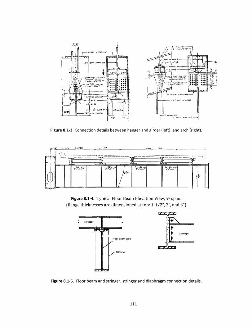
Figure 8.1‐3

(fla

Figure 8.1‐

3. Connection

Figure 8.1‐4.

angethickne

5. Floor beam

n details betw

TypicalFloessesaredim

m and stringe

111

ween hanger a

orBeamElevmensionedat

er, stringer an

and girder (le

vationView,top:1‐1/2”,

nd diaphragm

eft), and arch

½span.2”,and3”)

m connection

(right).

details.

8.2 Frigo

Th

judgment

bridge str

support c

Fl

girder sec

composite

and horiz

stringers

details bu

of the su

direction

: Developme

he Frigo brid

t were made

ructural secti

ondition. The

loor beams a

ctions are ign

e with the st

zontal transla

it sat on. The

ut simply by a

uperstructure

translations a

Figure 8.1‐

Figure 8.

ent of Three D

dge was not

in modelling

ons are mod

e complete m

are assumed

nored and th

ringers includ

ation are use

e knuckle joi

assuming the

e is idealized

and the other

‐6. Shear con

.2‐1. 3D FEM

Dimensional

load tested.

the Frigo brid

delled exactly

odel of the b

rigidly conne

he section is

ding the regio

ed to model

nt section at

arch is rigidl

d as simple

r end free in l

112

nector spacin

of Leo Frigo

Finite Eleme

Idealizations

dge just as in

y, assumption

ridge is diagr

ected with th

assumed co

on over floor

l the interac

t the arch an

y connected

roller‐pinned

longitudinal t

ngs above str

Memorial Bri

nt Model.

s and simplif

the other tw

ns are made

rammed in Fig

he tie girder

ntinuous. Th

r beams. Link

ction betwee

d girder join

with the tie g

d supported,

translation.

ingers.

idge.

fications base

wo arch bridge

regarding the

gure 8.2‐1.

box sections

e concrete d

k elements co

en the concr

ts are not m

girder. The b

i.e. one en

ed on engine

es. While the

e connection

s. Splices bet

deck was ass

onstraining ve

ete deck an

modeled with

oundary con

d constrainin

eering

e main

ns and

tween

umed

ertical

d the

exact

dition

ng all

113

8.3 Frigo: Impact of OSOW Vehicles.

Analysisresultsfromthebridgemodelforthecriticalmemberswithmaxstresslevelsforeachstructuralgroupunderare listed inTable8.3‐1 for theHL‐93notional loadingand inTable8.3‐2fortheOSOWvehicles.Witha40ft.wideroadwayineachdirection,sixlanesofHL‐93loadingcouldbeapplied.OnlyoneOSOWtruckwasassumedonthebridgeatanytime.TheOSOWvehiclenotationisasusedpreviously:

Single312 represents the 312 kips gross weight single trailer, Single446 represents the 446 kips gross weight single trailer, Dual486 represents the 486‐kip gross weight dual trailer, Dual500 represents the 500‐kip gross weight dual trailer.

The frame numbers listed in the tables are element numbers in the analytic model. A key to the

member locations is shown in Figure 8.3‐1.

Table 8.3‐1. Max stress results in each structural group under factored Dead+ HL‐93 loading.


Girder

Frame 280

Max Moment(kip‐ft)

16,481

Axial Force (kip)

‐3029

Stress (ksi)

36.9


3870


2933 21.4

Arch

Frame 662

Max Moment

4206

Axial Force

‐3944 ‐23.5

Frame 701 Min Axial Force

‐4988


1678 ‐21.4

Floor Beam

Frame 115

Max Moment

13,685

Axial Force

‐117 ‐24.7


564


7735 16.3

Stringer

Frame 1720

Min Moment

‐1020

Axial Force

263 52.4


274


565 33.0

Hanger

893

Max Axial

517 85

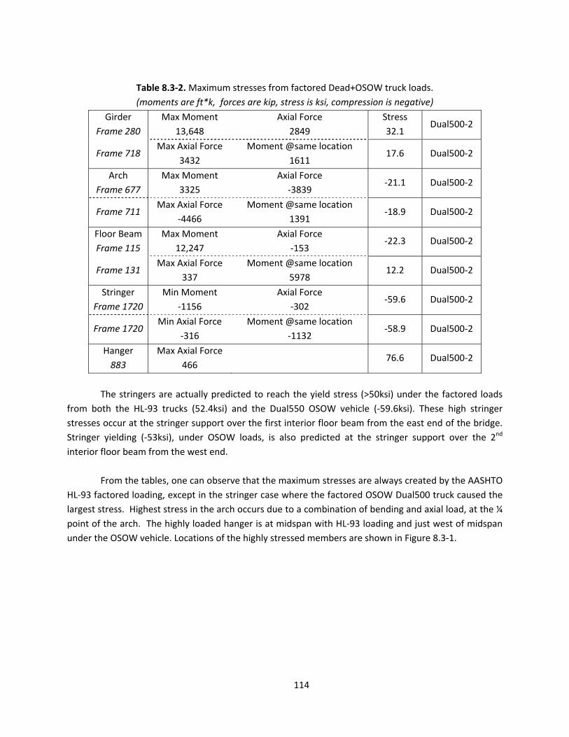
114

Table 8.3‐2. Maximum stresses from factored Dead+OSOW truck loads.


Girder

Frame 280

Max Moment

13,648

Axial Force

2849

Stress

32.1 Dual500‐2


3432


1611 17.6 Dual500‐2

Arch

Frame 677

Max Moment

3325

Axial Force

‐3839 ‐21.1 Dual500‐2


‐4466


1391 ‐18.9 Dual500‐2

Floor Beam

Frame 115

Max Moment

12,247

Axial Force

‐153 ‐22.3 Dual500‐2


337


5978 12.2 Dual500‐2

Stringer

Frame 1720

Min Moment

‐1156

Axial Force

‐302 ‐59.6 Dual500‐2


‐316


‐1132 ‐58.9 Dual500‐2

Hanger

883

Max Axial Force

466 76.6 Dual500‐2

The stringers are actually predicted to reach the yield stress (>50ksi) under the factored loads

from both the HL‐93 trucks (52.4ksi) and the Dual550 OSOW vehicle (‐59.6ksi). These high stringer

stresses occur at the stringer support over the first interior floor beam from the east end of the bridge.

Stringer yielding (‐53ksi), under OSOW loads, is also predicted at the stringer support over the 2nd

interior floor beam from the west end.

From the tables, one can observe that the maximum stresses are always created by the AASHTO

HL‐93 factored loading, except in the stringer case where the factored OSOW Dual500 truck caused the

largest stress. Highest stress in the arch occurs due to a combination of bending and axial load, at the ¼

point of the arch. The highly loaded hanger is at midspan with HL‐93 loading and just west of midspan

under the OSOW vehicle. Locations of the highly stressed members are shown in Figure 8.3‐1.

Figure8.3‐‐1.Planview

wsofFrigobr

115

ridgeshowin

nglocationsoofhighlystreessedmembe

ers.

116

9. SIMPLIFIED ANALYSIS METHODS FOR MEMBERS IN COMPLEX BRIDGES

The comprehensive calibrated 3D FEMs are generally thought to be accurate in the estimation

of the behavior of the complete structure as well as that of each individual component. Building and

running full scale 3D bridge FEMs, however, is time‐consuming and error‐prone due to the complexity of

many structures. Since critical information (e.g., required floor beam or stringer strength under certain

super loads) may not be available to bridge authorities when needed to support decisions regarding

allowing permit loads to cross a bridge, simplified methods for checking the force impact on members

are of interest.

The development of simplified analysis methods is included in this section to allow quick

estimation of future OSOW loading effects on critical bridge members. The focus here is on the

development of simple 2D models that can replicate the force estimates found in complicated 3D FEM

analysis.

As a first step – the results of the FEM analyses are reviewed to identify members that may be

critical for controlling the size or geometry of permit loads that can be carried by the complex arch and

bascule bridge structures examined earlier. Then the development of simplified 2D models will be

described in detail.

9.1: Critical Elements in Arch and Bascule Bridges.

The bridge elements that exhibited the highest stresses under factored HL‐93 and OSOW

vehicles are listed in Tables 9.1‐1&2. Under HL‐93 loading the capacity in all of the bridges is controlled

by either the stringer peak stress or the floor beam peak stress. The stringer controlled in the Marinette

bascule, Cameron tied arch and Frigo tied arch. The girders, arches or hangers did not control in any

bridge.

With loading from the selected OSOW vehicles the controlling member is not as consistent. For

both bascule bridges, however, the main bascule girder capacity controlled the bridge’s capacity. The

floor stringer is still the controlling member in the two tied arches: Cameron and Frigo. The OSOW

capacity of the Chippewa arch truss is limited by the capacity of the diagonal hangers.

Based on these results, developing a simplified method for estimating permit vehicle effects on

the bridge stringers and floor beams appears to be most critical since they control capacity in seven of

the 10 cases for the bridges with HL‐93 and OSOW loading. While OSOW loading is of prime interest, the

HL‐93 design loading provides a familiar basis for comparison. The following sections will look at

simplified methods to work with each of the bridges as a step in developing an overall method that may

apply to multiple bridge types.

117

Table 9.1‐1. Comparison of element peak stresses in members, shown as % of yield for HL‐93 loads.

HL‐93 induced member stress given as % of the yield stress:

member

type:

Marinette

bascule

Winneconne

bascule

Cameron

tied arch

Chippewa

truss arch

Frigo

tied arch

floor

stringer

81% 64% 72% 36% 104%

floor beam 64% 119% 36% 61% 50%

girder 61% 56% 58% 58% 74%

arch na na 50% 58% 48%

hanger na na 51% 56% 85%

(Shaded cells indicate element that controls capacity of that bridge.)

Table 9.1‐2. Comparison of element peak stresses in members, shown as % of yield for OSOW loads.

OSOW induced member stress given as % of the yield stress:

member

type:

Marinette

bascule

Winneconne

bascule

Cameron

tied arch

Chippewa

truss arch

Frigo

tied arch

floor

stringer

44% 33% 68% 40% 120%

floor beam 47% 64% 34% 50% 44%

girder 78% 69% 64% 52% 64%

arch na na 54% 50% 42%

hanger na na 54% 57% 77%

(Shaded cells indicate element that controls capacity of that bridge.)

9.2: Marinette Bascule Bridge ‐ Simplified 2D Methods.

The nature of the bascule bridge and the joint between the two opening leafs of the bascule

creates complexity. These joints need to be considered as “hinges” that can transfer vertical shear force

from one leaf to the other, but no moment. Most simplified bridge analysis methods do not

accommodate placement of a hinge in a span. A further complication comes if the joint is not tight and

some displacement of one leaf is required before shear transfer occurs. In this condition the bridge is a

non‐linear structural system.

The bascule bridge commonly contains three main members to be examined: the bascule girder,

floor beams, and stringers. Generally there are only two bascule girders, one on either side of the

roadway. The capacity of these girders controlled the bridge capacity in the two bridges examined here

when loaded with OSOW trucks. In the 3D FEM analyses, the HL93 and OSOW Dual500‐2 trailer (500kip)

were the two trucks that induced the highest stresses in the Marinette girders. The same trucks are used

118

in the 2D girder analyses here. Stringers controlled the bridge capacity under HL‐93 load and stringer

behavior will be examined first.

Stringer Analysis

Wheel loads are carried on the metal bridge deck and transferred to the longitudinal stringers.

Stringers in the Marinette Bridge span 171 inches (14.25ft) between floor beams and are alternately

continuous (i.e. each stringer is continuous over 2 spans on 3 floor beams, but the simple supported

ends are alternated between adjacent stringers). Some of the Marinette bridge stringers between floor

beams 4 and 5 (close to the mid joint) are non‐continuous – are just simply supported with a 171inch

span. These are the critical stringers for positive moment since there is no continuity, and negative end

moment, at either end.

The first step in the analysis is to select the position along the length of the selected stringer to

position the truck load to induce the largest bending moment. This can easily be done using simple

software such as PCBridge[6] or QConBridge[7]. Alternately the simple rule that the resultant total load

vector and the nearest wheel should be equidistant from the center of span can be used if a single

simple span stringer is investigated. The locations are as follow.

HL93 Truck: Maximum truck moment is found when the back wheel is located at midspan of a

non‐continuous stringer, 7.125 ft. from left support. The moment is 57ft‐k.

Dual500‐2 Trailer: The wheel line moment, a negative moment, was found over an interior 2

span floor beam support. As described earlier, the axle spacing of the trailer for the Dual500‐2 truck is

constant at 5ft. along the last 60ft. of the truck, the heavier part with 32k per axle set, 8k per wheel, on

two adjacent trailers. The two trailers are only 2ft. apart. The maximum positive span moment is 35.2ft‐

k and minimum negative moment is ‐42.9ft‐k.

To estimate the total truck moment carried by any stringer an attempt was made to use a

wheel load distribution factor. The AASHTO Standard Specifications Section [9] 3.23.2.3.1.5 factor to use

for cases with concrete flooring supported by 4 or more steel stringers was tried as a method to

estimate the portion of the wheel load that goes into the stringer. The older value was used because the

7th Ed. AASHTO LRFD Bridge Design Specifications [2] does not include a similar equation. The Standard

Spec. equations for the distribution factor are as follows:

5.5

4 0.25 ∗

Where, S is the distance in feet between outside and adjacent interior stringers. The first

equation is used when S is 6ft. or less, the second for over 6ft. The truck wheel line load moment is

multiplied by this factor to estimate the portion of a wheel line resisted by a single stringer. The spacing

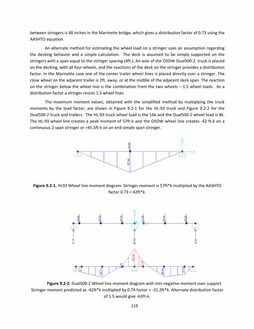
between

AASHTO e

A

the decki

stringers w

on the de

factor. In

close whe

on the str

distributio

Th

moments

Dual500‐2

The HL‐93

continuou

Figure 9

F

Stringer m

stringers is 48

equation.

n alternate m

ng behavior

with a span e

cking, with a

the Marinett

eel on the adj

ringer below

on factor a st

he maximum

by the load

2 truck and tr

3 wheel line

us 2 span strin

9.2‐1. HL93 W

Figure 9.2‐2.

moment pred

8 inches in th

method for es

and a simple

equal to the s

ll four wheels

te case one o

jacent trailer

the wheel li

ringer resists

m moment va

factor, are

railers. The H

creates a pea

nger or +45.5

Wheel line mo

Dual500‐2 W

dicted as ‐42f

he Marinette

stimating the

e calculation

stringer spacin

s, and the rea

of the center

is 2ft. away,

ne is the com

1.5 wheel lin

alues, obtaine

shown in Fig

HL‐93 truck w

ak moment o

5ft‐k on an en

ment diagram

factor

Wheel line mo

ft*k multiplied

of 1.5 w

119

bridge, which

e wheel load

. The deck i

ng (4ft.). An a

actions of the

trailer whee

or at the mid

mbination fro

nes

ed with the s

gure 9.2‐1 fo

wheel load is t

of 57ft‐k and

d simple span

m. Stringer m

r 0.73 = 42ft*

ment diagram

d by 0.74 fact

ould give ‐63

h gives a distr

on a stringer

is assumed t

axle of the OS

e deck on the

l lines is plac

ddle of the ad

om the two w

simplified me

r the HL‐93

the 16k and t

the OSOW w

n stringer.

moment is 57ft

k.

m with min ne

tor = ‐31.2ft*

ft‐k.

ribution facto

r uses an assu

to be simply

SOW Dual500

stringer prov

ced directly o

djacent deck

wheels – 1.5 w

ethod by mu

truck and Fig

the Dual500‐2

wheel line cre

t*k multiplied

egative mom

*k. Alternate d

or of 0.73 usin

umption rega

supported o

0‐2 truck is p

vides a distrib

ver a stringe

span. The rea

wheel loads.

ultiplying the

gure 9.2‐2 fo

2 wheel load

eates ‐42 ft‐k

d by the AASH

ent over supp

distribution f

ng the

arding

on the

placed

bution

r. The

action

As a

truck

or the

is 8k.

k on a

HTO

port.

actor

120

Note that the 0.73 distribution was used. That AASHTO factor was originally defined based on

truck loadings with wheels spaced at 6ft. on center on the axles. The dual trailer actually has wheels

closer together, spaced at 4ft. on an axle and 2ft. between wheels on two trailers. It is expected that

using the AASHTO factor with the OSOW truck would underestimate the total wheel load resisted by a

single stringer. A comparison of the simply estimated stringer moments and results from an accurate 3D

FEM analysis are listed in Table 9.2‐1.

Table 9.2‐ 1. Comparison of Marinette stringer moments ‐ accurate vs. approximate.

Bridge

Truck

Max. Moment

3D Model

(kip‐ft.)

Max. Moment

2D Analysis

(kip‐ft.)

% change vs.

3D Model

Marinette

HL93 42 42 0%

Dual500‐2, AASHTO df

alternate df

‐51 ‐31

‐63

‐39%

+23%

(df = distribution factor for portion of wheel line resisted by a stringer.)

Load and dynamic allowance factors as well as dead load are not included in Table 9.2‐1 values.

Moment values found in the 2D analysis for the HL93 trucks correlate very well with the 3D model. This

means that the simplified analysis may be used for predicting stringer forces when trucks having an axle

spacing similar to the HL‐93 truck (6ft.) are being considered. For the OSOW trucks, values found in the

AASHTO simplified analysis are up to a 40% smaller than the 3D Model. This shows that the AASHTO

equation used here does not work for the special axle configuration of the OSOW trucks on these

bridges. A simple alternate distribution, based on simple span deck calculations, overestimates the

negative moment by 23%. More data from other bridges and load configurations is needed in order to

create a general modification of the AASHTO equation for such trucks.

Floor Beam Analysis

For the floor beam analysis, reaction values estimated from the stringer analysis are used as

point loads applied directly to the floor beam. The maximum moment in the floor beam is calculated.

This is an approximate method because the reactions on the stringer are calculated with the same span

location of the truck as used for the stringer moment analysis. The true maximum reaction would occur

with a different truck position, usually with one axle directly above the floor beam. This approximation

will underestimate the reactions on the floor beam. Floor beams in the Marinette Bridge are 408 inches

(34ft.) long. The floor beam is assumed to be simply supported at its ends based on the web only

connection detailed in the bridge plans.

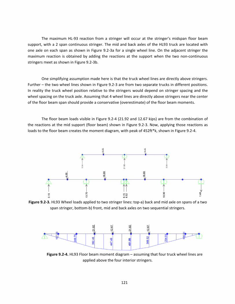
Th

support, w

one axle

maximum

stringers m

O

Further –

In reality

wheel spa

of the floo

Th

the reacti

loads to t

Figure 9.2

he maximum

with a 2 span

on each span

m reaction is

meet as show

One simplifyin

the two whe

the truck wh

acing on the t

or beam span

he floor beam

ions at the m

he floor beam

2‐3. HL93 Wh

span strin

Figure 9.2‐4

m HL‐93 react

n continuous

n as shown i

obtained by

wn in Figure 9

g assumption

eel lines show

heel position

truck axle. As

n should prov

m loads visibl

mid support (f

m creates the

heel loads app

nger, bottom‐

4. HL93 Floor

app

tion from a s

stringer. The

n Figure 9.2‐

adding the r

9.2‐3b.

n made here

wn in Figure 9

relative to t

suming that 4

vide a conserv

le in Figure 9

floor beam) s

moment dia

plied to two s

‐b) front, mid

beam mome

plied above th

121

stringer will o

e mid and ba

3a for a sing

reactions at t

is that the tr

9.2‐3 are from

the stringers

4 wheel lines

vative (overes

.2‐4 (21.92 a

shown in Figu

gram, with pe

stringer lines:

d and back axl

ent diagram –

he four interi

occur at the

ack axles of th

gle wheel line

the support

uck wheel lin

m two separa

would depen

are directly a

stimate) of th

nd 12.67 kip

ure 9.2‐3. No

eak of 452ft*

: top‐a) back

les on two se

– assuming th

or stringers.

stringer’s mi

he HL93 truc

e. On the adj

when the tw

nes are direct

ate trucks in d

nd on stringe

above stringe

he floor beam

s) are from t

ow, applying

*k, shown in F

and mid axle

equential strin

hat four truck

idspan floor

k are located

jacent stringe

wo non‐contin

tly above strin

different posi

er spacing an

ers near the c

m moments.

he combinat

those reactio

Figure 9.2‐4.

on spans of a

ngers.

wheel lines a

beam

d with

er the

nuous

ngers.

itions.

nd the

center

ion of

ons as

a two

are

R

set of stri

directly ab

trailer axl

spaced st

resisted b

distribute

Figure 9.2

H

D

Bridg

Marine

Ta

factors as

are up to

good tool

due to th

the full tr

load com

assumed

eactions from

inger analyse

bove four str

les and the t

tringer loadin

by stringers o

ed. The OSOW

2‐5. Combinin

L‐93:

ula500‐5:

Figure 9.2‐5.

Table 9.2‐

e

ette Dua

able 9.2‐2 co

s well as dead

15% greater

l to estimate

e approximat

uck loads we

ing from the

limited locati

m a Dual500‐6

es (same proc

ingers near m

trailers are a

ng on the flo

ther than the

W loading mo

ng both mom

1052ft*k

867ft*k

OSOW Dual5

from the t

‐ 2. Comparis

Truck

HL93

al Trailer 1‐6

ompares floo

d load are no

r than the 3D

the truck ind

te distributio

ere transferre

e stringers w

ions.

6 trailer set a

cedure as for

midspan of th

t 6ft. spacing

oor beam, th

e center four

ment diagram

ments with the

500‐6 Floor b

two trailers a

on of Marine

Max. Mo

3D Mode

ft.)

394

587

or beam est

ot included in

D values, a co

duced forces

on of the load

ed by just the

will be distrib

122

re found in a

r the HL93 tr

e floor beam

g, this may b

ough in reali

and the load

m, with peak

e LRFD impac

eam moment

re applied ab

tte floor beam

oment

el (kip‐

)

M

2

4

7

imated mom

n the table va

onservative re

in floor bea

d on the floo

four stringer

uted along t

similar mann

uck), assumin

. Since wheel

be an accept

ity some of

ds on the floo

of 642.4ft*k,

ct factor and l

t diagram – a

bove four strin

m moments ‐

Max. Momen

2D Analysis (k

ft.)

452

642

ments. Again

alues. Mome

esult. The sim

ms. The erro

r beams from

rs near midsp

the entire flo

ner. Reaction

ng the 4 trail

ls are spaced

table represe

the truck loa

or beam shou

, for the floor

load factor w

assuming that

ngers.

‐ accurate vs.

nt

ip‐

% c

3

load and d

ent values fro

mplified analy

or in simplifie

m the stringe

pan of the flo

oor beam an

s are found f

ler wheel line

at 4ft. on the

entation of th

ads would al

uld be more w

r beam is sho

ould produce

t four wheel l

approximate

change vs.

D Model

+15%

+9%

ynamic allow

om the 2D an

ysis seems to

ed results cou

rs. In our ana

oor beam. The

nd not only i

rom a

es are

e dual

he 4ft

so be

widely

own in

e:

ines

e.

wance

nalysis

o be a

uld be

alysis,

e true

n the

123

Girder Analysis

Girder force analysis might be simplified by modeling a girder as a 2D uniform prismatic beam

with a fixed support at each end and connected in the middle by a link element only capable of

transferring vertical loads as diagrammed in Figure 9.2‐6. Three important assumptions are made in this

analysis approach. First, most bascule bridge girders are not uniform prismatic beams; their cross

section varies along the length. Since this is a symmetric model and nearly determinate, the girder

section variation has little impact. An “exact” analysis, assuming the girder depth varied linearly along its

length was performed, but results proved that there was a change of less than 1% with respect to the

average moment of inertia analysis. Secondly, the joint between leafs may have an initial gap that allows

one leaf to move relative to the other. If a gap exists, then the varying girder stiffness becomes more

important and the structure is indeterminate. The simplified model assumes no gap exists. And finally, in

doing 2D modeling an assumption must be made regarding the portion of truck loading that is

transferred to each of the two bridge girders.

Figure9.2‐6.Simple2Dmodelofbasculebridgewithhingedjointatcenter.

The length of each girder in the Marinette Bridge was taken from the plans as 791 inches

(65.9ft). A girder is modelled with uniform stiffness, fixed at the abutment and with a hinge to the

adjacent leaf’s girder at midspan exactly as laid out in Figure 9.2‐6.

In the HL93 analysis two trucks are assumed to be on the bridge simultaneously in symmetric

transverse positioning. Both trucks are placed on one leaf. With the symmetric layout, one girder would

collect the full load from one truck.

For the Dual500‐2 truck, only one truck is assumed to be allowed on the bridge and it is placed

adjacent to one edge of the roadway. To determine the portion of truck load that would be collected by

a single girder, a supplementary hand calculation with the floor beam as a simply supported span is

conducted. The Dual500‐2 wheels of one axle line are placed on a transverse floor beam and the

reactions from the floor beam on the girder are calculated by hand. In the Marinette bridge the girder

closer to the dual trailer received 64% of the total axle weight, while the furthest girder received only

36%. This same distribution is then assumed to exist for all the truck axles.

Once the portion of truck loading (HL‐93 or Dual500‐2) carried by each girder was determined,

the portion of the truck axles loads were applied directly on the girder in the model described earlier as

124

point loads at each axle location. As a simplification, the loads were applied at the axle locations rather

than attempting to find how much load goes on each floor beam and then applying the loads on the

girder at the floor beam locations. The maximum moments in the girder can then be calculated, but due

to the indeterminacy created by the hinge, an analysis software such as SAP200 or CSiBridge is best

used. In this case the calculated moments are:

HL93: ‐2118ft*k or as a factored load: ‐4930ft*k

Dual500‐2: ‐7044ft*k or as a factored load: ‐9509ft*k

The girder moments from the simplified method are compared with those obtained during the

accurate 3‐D FEM analysis in Table 9.2‐3. Load and dynamic allowance factors as well as dead load are

not included in the table results. The values in parenthesis for the 2D analysis column are results from a

model that considered a linear variation of the cross section between support and mid joint, rather than

a constant cross section. So, in order to simplify the analysis, the results using an average cross sections

are used for reference when comparing the 2D versus the 3D data.

Results from the simplified analysis are very accurate for the HL93 trucks, with a variation of

only 3 percent. For the OSOW trucks, the simplified values are 21 percent greater than the values from

the complex 3D models. These conservative estimates for OSOW trucks may be good when rating these

complex bridges for permit loads. The difference in values might be explained by the simple idealized

method of estimating what portion of a truck load is carried to each girder in the bascule bridge.

Table 9.2‐3 . Comparison of Marinette girder moments accurate vs. approximate.

Bridge

Truck

Max. Moment

3D Model (kip‐

ft.)

Max. Moment

2D Analysis (kip‐

ft.)

% change vs.

3D Model

Marinette

HL93 ‐2185 ‐2118 (‐2139) ‐3%

Dual500‐2 ‐5811 ‐7044 (‐7036) +21%

9.3: Winneconne Bascule Bridge ‐ Simplified 2D Methods

The Winneconne Bridge is the second of two bascule bridges examined during this study. It is

similar in overall design to the Marinette bascule with the same unique complexity that exists in most

bascule bridges.

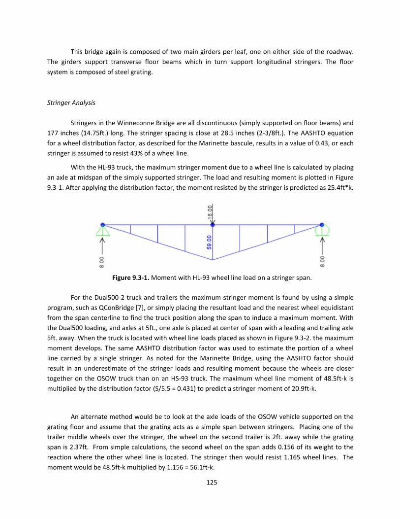
Th

The girde

system is

Stringer A

St

177 inche

for a whe

stringer is

W

an axle at

9.3‐1. Afte

Fo

program,

from the

the Dual5

5ft. away.

moment

line carrie

result in a

together

multiplied

A

grating flo

trailer mi

span is 2.

reaction w

moment w

his bridge ag

ers support t

composed of

Analysis

tringers in the

es (14.75ft.) l

el distributio

s assumed to

With the HL‐93

t midspan of

er applying th

or the Dual50

such as QCon

span centerli

500 loading, a

. When the tr

develops. Th

ed by a singl

an underesti

on the OSOW

d by the distri

n alternate m

oor and assu

ddle wheels

37ft. From s

where the ot

would be 48.5

ain is compo

transverse flo

f steel grating

e Winneconn

ong. The stri

n factor, as d

resist 43% of

3 truck, the m

the simply su

he distributio

Figure 9.3‐1.

00‐2 truck an

nBridge [7], o

ine to find th

nd axles at 5f

ruck is located

e same AASH

le stringer. A

mate of the

W truck than

ibution factor

method would

me that the

over the stri

simple calcula

ther wheel lin

5ft‐k multiplie

sed of two m

oor beams w

g.

ne Bridge are

nger spacing

described for

f a wheel line

maximum stri

upported strin

n factor, the

Moment wit

nd trailers the

or simply plac

e truck posit

ft., one axle i

d with wheel

HTO distribut

As noted for

stringer load

on an HS‐93

r (S/5.5 = 0.43

d be to look

grating acts

nger, the wh

ations, the se

ne is located

ed by 1.156 =

125

main girders p

which in turn

all discontinu

is close at 2

the Marinett

.

nger momen

nger. The loa

moment resi

h HL‐93 whee

e maximum s

cing the result

ion along the

s placed at ce

line loads pla

tion factor wa

the Marinett

ds and resulti

3 truck. The m

31) to predict

at the axle lo

as a simple s

heel on the s

econd wheel

. The stringe

= 56.1ft‐k.

per leaf, one

n support lo

uous (simply

8.5 inches (2

te bascule, re

t due to a wh

ad and resulti

isted by the s

el line load on

stringer mom

tant load and

e span to indu

enter of span

aced as show

as used to es

te Bridge, us

ing moment

maximum wh

t a stringer m

oads of the O

span between

econd trailer

on the span

r then would

on either sid

ngitudinal st

supported on

2‐3/8ft.). The

esults in a valu

heel line is ca

ng moment i

stringer is pre

n a stringer s

ment is found

d the nearest

uce a maxim

n with a leadin

wn in Figure 9.

stimate the p

sing the AASH

because the

heel line mom

moment of 20

OSOW vehicle

n stringers.

r is 2ft. away

adds 0.156 o

d resist 1.165

de of the road

tringers. The

n floor beams

AASHTO equ

ue of 0.43, or

lculated by p

is plotted in F

edicted as 25.

pan.

by using a s

wheel equid

um moment.

ng and trailin

.3‐2. the max

portion of a w

HTO factor s

wheels are c

ment of 48.5

.9ft‐k.

e supported o

Placing one o

y while the g

of its weight t

5 wheel lines

dway.

floor

s) and

uation

r each

lacing

Figure

4ft*k.

simple

istant

. With

g axle

imum

wheel

hould

closer

ft‐k is

on the

of the

rating

to the

. The

A

illustrated

for that ty

the OSOW

stringers i

somewha

Th

stringers,

deck is a

analysis f

OSOW tru

Ta

Bridge

Winneco

Floor Bea

Fl

assumed

Analysis o

Fo

symmetri

come to

always fal

gain the sim

d in Table 9.3

ype of loadin

W loading oc

in the Winnec

at better, but

he alternate

overestimate

pparently dis

or a distribut

uck wheel line

able 9.3‐1 . C

e

nne Dual50

Dual50

(df =

m Analysis

loor beams i

to be simply

of the floor be

or the analy

cally in the t

the floor bea

lls directly ab

Figure 9.3

ple AASHTO

3‐1. HL‐93 re

ng with a 6ft.

ccurs, better

conne vs. the

unconservati

method, look

es the mome

stributing the

tion factor in

e distribution

Comparison of

Truck

HL93

00‐2 AASHTO

00‐2 alternat

distribution f

in the Winne

y supported b

eam moment

ysis with two

ransverse dir

ams through

ove a stringe

‐2. Dual500‐2

analysis for

esults are goo

axle spacing

than was s

e trailer whee

ive for evalua

king at wheel

nt by 124%. W

e load more

n the alternat

to stringers

f Winneconne

O df

te df

factor for port

econne Bridg

because the s

t follows the p

o HL93 truck

rection and n

the stringer

er. So the HL9

126

2 wheel line m

stringer mom

od since the

. The stringe

een with the

el spacing mak

ating permit t

l loads on the

With the clos

e efficiently t

te method. C

is needed.

e stringer mo

Max. Mome

3D Model

(kip‐ft.)

26

25

tion of wheel

ge are 342 in

sole connecti

procedure de

ks on the br

near the cent

r reactions. A

3 truck whee

moment on a

ments undere

assumed dist

er moment is

e Marinette

kes the assum

truck effects.

e grating floo

e stringer spa

than assume

Clearly an im

oments ‐ accu

ent

l

Max. M

2D A

(kip

2

2

5

l line resisted

nches (28.5ft

ion to the gir

escribed for th

ridge, assum

er of the floo

Again it is ass

els are assume

stringer span

estimates the

tribution fact

s underestima

bridge. The

med AASHTO

or and the flo

acing (2.37ft.

d using the

mproved meth

urate vs. appr

Moment

Analysis

p‐ft.)

%

25

21

56

by a stringer

t.) long. The

rder is throug

he Marinette

me that the

or beam span

sumed that a

ed to be spac

n.

e true mome

tor was deve

ated by 16%

closer spaci

distribution f

oor reaction o

) of this bridg

simple span

hod for estim

roximate.

% change vs.

3D Model

‐4%

‐16%

+124%

r.)

beams are

gh the beam

bascule.

trucks are p

n. The truck

a truck whee

ced at 4.75ft a

ent as

loped

when

ng of

factor

on the

ge the

deck

mating

again

web.

placed

loads

el line

apart,

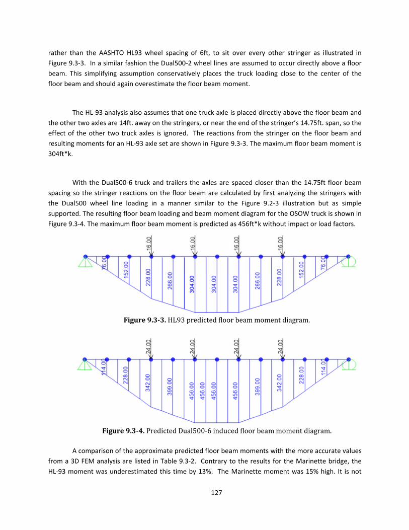
rather tha

Figure 9.3

beam. Th

floor beam

Th

the other

effect of

resulting

304ft*k.

W

spacing so

the Dual5

supported

Figure 9.3

A

from a 3D

HL‐93 mo

an the AASH

3‐3. In a simi

his simplifying

m and should

he HL‐93 ana

two axles are

the other tw

moments for

With the Dual

o the stringe

500 wheel li

d. The resulti

3‐4. The maxi

Figu

comparison

D FEM analys

oment was un

HTO HL93 wh

ilar fashion th

g assumption

d again overes

alysis also ass

e 14ft. away o

wo truck axles

r an HL‐93 axl

500‐6 truck a

r reactions o

ne loading i

ng floor beam

mum floor be

Figure9.

ure9.3‐4.Pr

of the approx

sis are listed

nderestimate

heel spacing

he Dual500‐2

n conservativ

stimate the fl

umes that on

on the stringe

s is ignored.

e set are sho

and trailers t

on the floor b

n a manner

m loading and

eam moment

3‐3.HL93pr

redictedDual

ximate predic

in Table 9.3‐2

ed this time b

127

of 6ft, to sit

wheel lines

ely places th

oor beam mo

ne truck axle

ers, or near th

The reaction

own in Figure

the axles are

beam are calc

similar to t

d beam mome

t is predicted

redictedfloo

l500‐6induc

cted floor bea

2. Contrary t

by 13%. The

over every

are assumed

he truck load

oment.

is placed dire

he end of the

ns from the s

9.3‐3. The m

spaced close

culated by fir

the Figure 9.

ent diagram f

as 456ft*k w

orbeammom

cedfloorbea

am moments

to the results

Marinette m

other stringe

to occur dire

ding close to

ectly above t

e stringer’s 14

stringer on th

maximum floo

er than the 1

rst analyzing

.2‐3 illustrati

for the OSOW

without impac

mentdiagram

ammomentd

s with the mo

s for the Ma

moment was

er as illustrat

ectly above a

the center o

he floor beam

4.75ft. span, s

he floor beam

r beam mom

14.75ft floor

the stringers

ion but as s

W truck is sho

t or load fact

m.

diagram.

ore accurate v

rinette bridge

15% high. It

ted in

a floor

of the

m and

so the

m and

ment is

beam

s with

simple

own in

ors.

values

e, the

is not

128

clear why the HL‐93 moment is underestimated in this case. The HL‐93 wheel lines were assumed to be

at double the stringer spacing, 4.75ft., rather than the actual 6ft. in the truck. This places all the wheel

lines close together and should still overestimate the floor beam moment. Apparently more geometric

configurations should be considered before adopting a simple method such as suggested here.

Table 9.3‐2 . Comparison of Winneconne floor beam moments ‐ accurate vs. approximate.

Bridge

Truck

Max. Moment

3D Model (kip‐

ft.)

Max. Moment

2D Analysis (kip‐

ft.)

% change vs.

3D Model

Winneconne

HL93 348 304 ‐13%

Dual500‐6 397 456 +15%

Girder Analysis

The Winneconne bascule girders are 474 inches (39.5ft.) long. The same procedure forsimple analysis described for the Marinette Bridge is used again. The girder distribution factorcalculated for theHL93truck,byhandcalculationonasimplysupported floorbeam, isagain1.0withtwoHL‐93trucks and0.75fortheDual500‐2OSOWvehicle.Themaximummomentsatthesupport forboth trucksare listed inTable9.3‐3.Thevalues inparenthesisare resultsestimatedusingalinearvariationofcrosssectionforthegirderalongitslengthratherthanaconstantcrosssection.

ThemomentcomparisoninTable9.3‐3showsHL‐93resultsnearlyidenticaltothoseofthe

Marinette girder when looking at the errors in values from the simple prediction method. Themethod is quite accurate for HL‐93 double truck loading with a symmetrical placement. Theapproximatemethod,however,overestimatestheportionofanOSOWtruckloadtransferredtoasinglegirderwhenthetruckisplacedtowardonesideofthebridge.

Table9.3‐3.ComparisonofWinneconnebasculegirdermoments‐accuratevs.approximate.

Bridge

Truck

Max. Moment

3D Model (kip‐

ft.)

Max. Moment

2D Analysis (kip‐

ft.)

% change vs.

3D Model

Winneconne

HL93 ‐1192 ‐1155 (‐1166) ‐3%

Dual Trailer 1‐2 ‐2700 ‐3481 (‐3482) +29%

129

9.4: Cameron Avenue Arch Bridge ‐ Simplified 2D Analysis Methods

In the Cameron Avenue arch bridge, all stringers are 7’10” apart and simply supported on floor

beams. While most are 23.25ft. long, the end spans are 25.25ft. long and therefore control for the max

bending moment due to the extra length.

Stringer Analysis

The PCBridge software is used to find where the HL‐93 and OSOW trucks should be placed along

the stringer span to create the maximum stringer moment. This could also be easily found using the

simple hand calculation method described with the Marinette and Winneconne bridge. The critical HL‐

93 location is with the truck driving from west to east with its back axle 9.25ft. from the west end of the

stringer and middle axle 2ft. from the east end. The front axle is off the stringer. The maximum truck

bending moment for a wheel line can be calculated by hand from the diagram in Figure 9.4‐1

and is 105.5ft‐kips. The AASHTO distribution factor, calculated as described previously, is 1.31 with

spacing greater than 6ft. The OSOW truck position is determined in a similar manner and the resulting

moments from a wheel line hand calculated. The same AASHTO distribution factor is used

If the alternate method is used for finding load distribution to a stringer, considering the deck as

simple spans with axle wheel loads applied, the factor for the Dual500‐2 truck would be 2.47 wheel lines

per stringer. It is calculate with one inner trailer wheel line over the stringer, the other wheel of that

axle 4ft. away on the deck to one side and the two wheel lines of the other trailer on the deck span to

the other side.

Figure 9.4‐1. HL‐93 truck position to cause max moment in stringer.

Predictedmomentestimates, without load or impact factors, are listed in Table 9.4‐1. The

AASHTO distribution coefficient works well for the HL‐93 truck but results in a 37% overestimate of

moment for the OSOW truck when using the AASHTO load distribution factor. The alternate distribution

factor, hand calculated looking at the deck as simple spans with an axle set of loads applied, would have

overestimated the moment by 158%.

Ta

Bridg

Camer

In

wheel line

LaCrosse

while the

Fi

at a floor

T

beam mid

moments

able 9.4‐ 1. C

e

on D

n order to in

es are over st

bridge as we

actual distan

igure 9.4‐2 sh

beam. The ca

F

The reactions

dspan are sh

are +294ft‐k

Comparison of

Truck

HL93

Dual500‐2

nduce maxim

tringers close

ll as the othe

nce between t

hows the HL‐

alculated reac

Figure 9.4‐2.

of the HL‐93

hown in Figu

and ‐520ft‐k

Figure 9.4

f Cameron st

Max. Mom

3D Mode

ft.)

138

125

Floor

um bending

to the cente

er arch bridge

the two whee

93 wheel line

ction on the s

HL‐93 truck p

3 (23.7k each

ure 9.4‐3. Wi

.

4‐3. HL‐93 str

130

ringer mome

ment

l (kip‐

M

2D

Beam Analys

moment in

r of the floor

es. The string

el lines of an

e loading pos

stringer is 23.

position on st

h) assumed to

ith a uniform

ringer reactio

nts ‐ accurate

Max. Moment

D Analysis (kip

ft.)

138

171

sis

the floor bea

beam. This is

ger spacings i

HL‐93 truck is

sition on strin

.7k per wheel

tringers to cre

o come from

m cross secti

ons as loads o

e vs. approxim

t

p‐

% ch

3D

+

am, again as

s a practical a

n these bridg

s 6ft. so the m

ngers to induc

l line.

eate max reac

m four of the

ion and fixed

on floor beam

mate.

hange vs.

D Model

0%

+37%

ssume that ve

assumption fo

ges are near 7

match is good

ce a large rea

ction.

stringers nea

d ends, the

m.

ehicle

or the

7.5ft.,

d.

action

ar the

beam

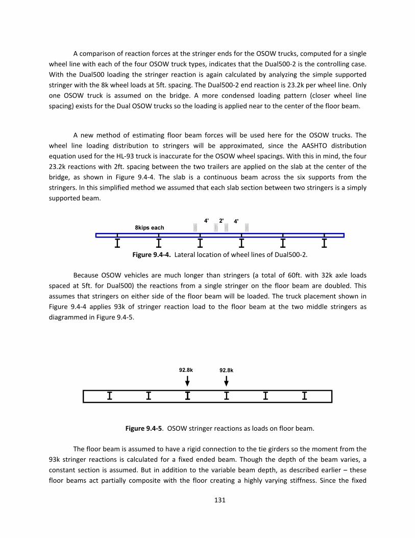
131

A comparison of reaction forces at the stringer ends for the OSOW trucks, computed for a single

wheel line with each of the four OSOW truck types, indicates that the Dual500‐2 is the controlling case.

With the Dual500 loading the stringer reaction is again calculated by analyzing the simple supported

stringer with the 8k wheel loads at 5ft. spacing. The Dual500‐2 end reaction is 23.2k per wheel line. Only

one OSOW truck is assumed on the bridge. A more condensed loading pattern (closer wheel line

spacing) exists for the Dual OSOW trucks so the loading is applied near to the center of the floor beam.

A new method of estimating floor beam forces will be used here for the OSOW trucks. The

wheel line loading distribution to stringers will be approximated, since the AASHTO distribution

equation used for the HL‐93 truck is inaccurate for the OSOW wheel spacings. With this in mind, the four

23.2k reactions with 2ft. spacing between the two trailers are applied on the slab at the center of the

bridge, as shown in Figure 9.4‐4. The slab is a continuous beam across the six supports from the

stringers. In this simplified method we assumed that each slab section between two stringers is a simply

supported beam.

Figure 9.4‐4. Lateral location of wheel lines of Dual500‐2.

Because OSOW vehicles are much longer than stringers (a total of 60ft. with 32k axle loads

spaced at 5ft. for Dual500) the reactions from a single stringer on the floor beam are doubled. This

assumes that stringers on either side of the floor beam will be loaded. The truck placement shown in

Figure 9.4‐4 applies 93k of stringer reaction load to the floor beam at the two middle stringers as

diagrammed in Figure 9.4‐5.

Figure 9.4‐5. OSOW stringer reactions as loads on floor beam.

The floor beam is assumed to have a rigid connection to the tie girders so the moment from the

93k stringer reactions is calculated for a fixed ended beam. Though the depth of the beam varies, a

constant section is assumed. But in addition to the variable beam depth, as described earlier – these

floor beams act partially composite with the floor creating a highly varying stiffness. Since the fixed

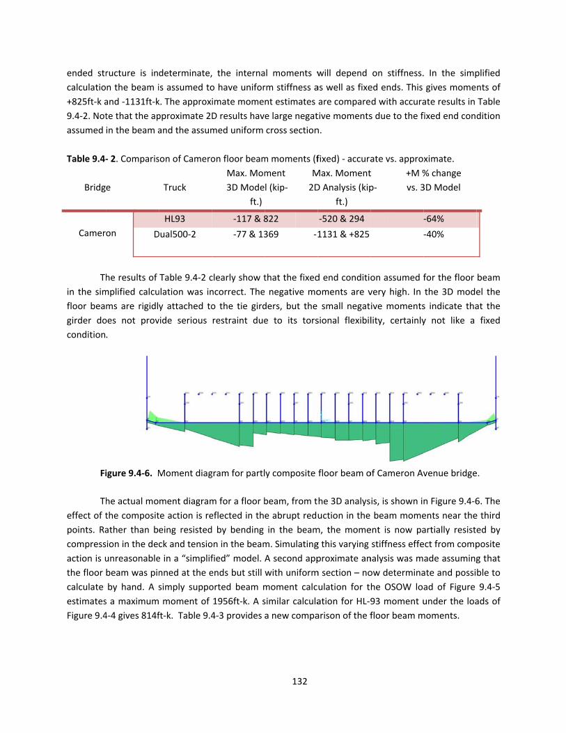
ended str

calculatio

+825ft‐k a

9.4‐2. Not

assumed

Table 9.4‐

Bridg

Camer

Th

in the sim

floor bea

girder do

condition

Fi

Th

effect of t

points. Ra

compress

action is u

the floor

calculate

estimates

Figure 9.4

ructure is in

n the beam i

and ‐1131ft‐k

te that the ap

in the beam a

‐ 2. Comparis

e

on D

he results of

mplified calcu

ms are rigidl

oes not prov

.

igure 9.4‐6. M

he actual mo

the composit

ather than b

sion in the dec

unreasonable

beam was pin

by hand. A s

s a maximum

4‐4 gives 814f

determinate,

is assumed to

k. The approx

pproximate 2

and the assum

son of Camero

Truck

HL93

Dual500‐2

Table 9.4‐2 c

ulation was in

y attached to

vide serious

Moment diag

ment diagram

te action is re

eing resisted

ck and tensio

e in a “simplif

nned at the e

simply suppo

moment of

ft‐k. Table 9.4

, the interna

o have unifor

imate mome

D results hav

med uniform

on floor beam

Max. Mom

3D Mode

ft.)

‐117 & 8

‐77 & 13

clearly show t

ncorrect. The

o the tie gird

restraint due

gram for partl

m for a floor b

eflected in th

d by bending

on in the beam

fied” model.

ends but still

orted beam m

1956ft‐k. A s

4‐3 provides

132

al moments w

rm stiffness a

nt estimates

e large negat

cross section

m moments (f

ment

l (kip‐

M

2D

822

369 ‐1

that the fixed

negative mo

ders, but the

e to its tors

y composite

beam, from t

e abrupt redu

in the beam

m. Simulating

A second app

with uniform

moment calc

similar calcula

a new compa

will depend

as well as fixe

are compare

tive moments

n.

fixed) ‐ accura

Max. Moment

D Analysis (kip

ft.)

‐520 & 294

1131 & +825

d end conditio

oments are v

small negat

sional flexibil

floor beam o

he 3D analys

uction in the

m, the mome

g this varying

proximate an

m section – no

ulation for t

ation for HL‐9

arison of the f

on stiffness.

ed ends. This

d with accura

s due to the f

ate vs. appro

t

p‐

+M %

vs. 3

on assumed f

very high. In

ive moments

lity, certainly

of Cameron Av

is, is shown i

beam mome

ent is now pa

stiffness effe

nalysis was m

ow determina

he OSOW lo

93 moment u

floor beam m

. In the simp

gives mome

ate results in

fixed end con

ximate.

% change

3D Model

‐64%

‐40%

for the floor

the 3D mode

s indicate tha

y not like a

venue bridge

n Figure 9.4‐6

ents near the

artially resist

ect from comp

ade assuming

ate and possi

ad of Figure

under the loa

moments.

plified

nts of

Table

dition

beam

el the

at the

fixed

e.

6. The

e third

ed by

posite

g that

ble to

9.4‐5

ads of

133

Table 9.4‐ 3. Second comparison of Cameron floor beam moments (pinned) ‐ accurate vs. approximate.

Bridge

Truck

Max. +Moment

3D Model (kip‐

ft.)

Max. +Moment

2D Analysis (kip‐

ft.)

+M % change

vs.3D Model

Cameron

HL93 822 814 ‐1%

Dual500‐2 1369 1956

+43%

Examining the results in Table 9.4‐3 it is apparent that the simplified estimate of floor beam

moments caused by an OSOW truck are inadequate with a 43% excess. This is attributed to the inability

of the simple model to capture the effect of partial composite action, changing the beam stiffness, and

the partial rigidity of the end support as influenced by the torsional rigidity of the tie girder.

9.5: Chippewa Arch Bridge ‐ Simplified 2D Analysis Methods

Stringer Analysis

The stringer configuration of the Chippewa River arch bridge is nearly the same as the Cameron

Avenue Bridge (spacing 7’‐5” vs 7’‐10” and span 25’ vs 23.25’ for Chippewa vs Cameron). The same

results for maximum moment due to a wheel line can be assumed. The final stringer maximum moment

is different, however, because the stringers are 7’‐5” apart slightly changing the distribution factor.

Stringer moment estimation results are shown in Table 9.5‐1.

Table 9.5‐ 1. Comparison of Chippewa stringer moments ‐ accurate vs. approximate.

Bridge

Truck

Max. Moment

3D Model (kip‐

ft.)

Max. Moment

2D Analysis (kip‐

ft.)

% change vs.

3D Model

Chippewa

HL93 131 134 +2%

Dual500‐2 142 165 +16%

Again, it can be seen that the use of the distribution factor works for the HL‐93 loading

configuration, but is conservative for the OSOW configuration.

134

Floor Beam Analysis

Following a procedure similar to that used in the Cameron Avenue bridge analysis – peak wheel

line reactions from the stringers were calculated, slab transfer of wheel lines to stringers, and stringer

reaction on floor beams from wheel lines were estimated. In the Dual500 loading case the four trailer

wheels were placed with each trailer to one side of the stringer near midspan of the floor beam. Then

assuming that the deck was simple spans, the distribution of the Dual500 load to the supporting

stringers was hand calculated. The idealization in this calculation is shown in Figure 9.5‐1 with the

adjacent deck span to be superimposed with the shown span. The middle stringer received 2.38 wheel

lines and the two adjacent stringers received 0.81 wheel lines each.

2989

29 4889

1.19

2 0.81

Figure 9.5‐1. Model for distribution of Dual500 wheel line loads to stringers.

The Dual500 8k wheels spaced at 5ft. were assumed to extend over two stringer spans, with one

axle directly above the floor beam. The model for this is detailed in Figure 9.5‐2. A hand calculation of

the reaction at the floor beam gave a force of 24k per such wheel line. A second stringer, to the right of

the one shown, would contribute another 16k to the reaction for a total of 40k.The previous factors,

2.38 and 0.81, were applied to the wheel line 40k reaction to calculate the loads applied to a floor beam

by the stringers.

Figure 9.5‐3 shows the stringer loads applied to the floor beam of the Chippewa Bridge for the

HL‐93 and OSOW Dual500‐2 loadings. The HL‐93 includes three lanes loaded and a multi‐presence factor

of 0.85 with equal distribution to all stringers. One OSOW truck is assumed with no multi‐presence

factor and the distribution factors calculated above. Results for maximum moments by performing a

floor beam analysis assuming fixed ends are shown in Table 9.5‐2.

135

8 ∗ 525

1025

1525

2025 1 8 ∗ 3 24

Figure 9.5‐2. Dual500 stringer reaction on floor beam support.

Figure 9.5‐3. Stringer reactions on floor beams for the HL‐93 loading (at top) and the OSOW Dual500‐2

loading (bottom) looking toward East at a Chippewa cross section.

Table 9.5‐ 2. Comparison of Chippewa floor beam moments ‐ accurate vs. fix end approximate.

Bridge

Truck

Max. Moment

3D Model (kip‐

ft.)

Max. Moment

2D Analysis (kip‐

ft.)

+M % change

vs.3D Model

Chippewa

HL93 ‐‐244, +446 ‐601, +308 ‐30%

Dual500‐2 ‐225, +592 ‐1052, +815 +38%

The results of the simple analysis in Table 9.5‐2 look quite poor compared to the 3D analysis

results. As in the previous Cameron Avenue bridge analysis, the assumption of fixed ends in the simple

floor beam analysis overestimates the size of the negative end moments. This is again attributable to the

torsional stiffness of the tie girders providing less than a fixed end condition. In the cast of the Dual500

OSOW loading, however, the simplified method appears to overestimate both positive and negative

moments. Apparently the actual loads applied near the center of the floor beam in this case are reduced

and loads must be redistributed to adjacent stringers and floor beams. This distribution is a function of

the relative stiffnesses of each of those members and is not represented in the simplified model. Figure

9.5‐4 shows the 3D moment diagram for a floor beam under Dual500‐2 loading along with the predicted

simplified fixed end moment diagram.

F

Th

of the floo

each strin

developin

Avenue b

conducted

as shown

F

Table 9.5‐

Bridg

Chippe

igure 9.5‐4. C

mo

he 3D analys

or beam com

nger, where

ng with the flo

ridge. In an a

d with the flo

in Figure 9.5‐

igure 9.5‐5. C

mo

‐ 3. Comparis

e

wa D

Comparison o

oment diagram

is moment di

mpared to the

the deck is

oor beam – r

attempt to im

oor beam end

‐5 and Table

Comparison o

ment diagram

son of Chippe

Truck

HL93

Dual500‐2

of 3D FEM pre

m from the fi

for the Dua

iagram of Fig

e results from

composite w

reducing the

mprove the sim

d pinned inste

9.5‐3.

of 3D FEM pre

m from the pi

for the Dua

wa floor beam

Max. Mom

3D Mode

ft.)

‐‐244, +4

‐225, +5

136

edicted floor

xed end simp

al500‐2 OSOW

ure 9.5‐4 disp

m the simplifie

with the strin

floor beam m

mplified mod

ead of fixed. T

edicted floor

in ended simp

al500‐2 OSOW

m moments ‐

ment

l (kip‐

M

2D

446

592

beam mome

plified analysi

W truck loadin

plays smaller

ed analysis. B

nger, some

moments as s

del prediction

The positive m

beam mome

plified analys

W truck loadin

‐ accurate vs.

Max. Moment

D Analysis (kip

ft.)

+892

+1809

ent diagram (s

is (red dash)

ng.

r moments al

But it addition

composite d

seen previous

n a second se

moment incre

ent diagram (s

is (red dash)

ng.

pinned appr

t

p‐

+M %

vs.3

+

+

solid green) w

ong the full l

nally shows th

eck action is

sly in the Cam

et of analyses

eases substan

solid green) w

roximate.

% change

3D Model

+100%

+205%

with a

ength

hat at

s also

meron

were

ntially

with a

137

Neither of the simplified floor beam models for the Chippewa bridge are satisfactory for

predicting effects of HL‐93 loading or the Dual500‐2 OSOW truck loading. The best model, assuming the

beam has fixed ends, underestimated positive moments by 30% for the HL‐93 truck and overestimated

positive moments by 38% for the Dual500 load. In both loadings the negative end moments were

overestimated. It is clear from inspecting the accurate 3D FEM response results that the floor beam is

only partially restrained in bending at its ends, due the torsional flexibility of the tie girder, acts partially

composite with the concrete deck and likely resists less load with more load distribution through the

bridge structural system than assumed in the simplified model. An accurate estimate of floor beam

moments appears to be difficult using a simplified approach without considerable further study of the

behavior of these complex bridge systems.

9.6: Leo Frigo Memorial Bridge ‐ Simplified 2D Analysis Methods

An immediate added complexity in predicting forces in the Frigo bridge comes from theunusualstringersystememployedwhileprovidinganexpansionjointnearmidspanofthebridgedeck.Thestringersruncontinuouslyoverthetopofthefloorbeamsinthisbridge.But,therearetwoseparatecontinuousstringersectionscomingfromeachendofthebridgewithaspecialjointnearthemiddleofthebridge.Thejointisbasicallyashiplapsupportwithastubcantileverstringerextendingoutfromthefloorbeamnearmidspanandthelongstringerinthespansimplysupportedonthisstub.

Stringer Analysis:

In developing a simplified model of this stringer system the first step was to model one whole

stringer, using the CSiBridge software, with the stringer simply supported (but continuous) over each

floor beam but with a pin joint at the stub cantilever. An HL‐93 truck wheel line was run along the

stringer to find the truck position causing a maximum moment. The stringers are spaced at 9.12ft., wider

than the HL‐93 wheel spacing of 6ft. With 3 loaded lanes and 5 stringers, it might be reasonable to

assume that each stringer carries an equal portion of the six HL‐93 wheel lines – or 1.2 wheel lines each.

From the resulting moment envelope it was clear that the 6th full stringer span from the west

end, the first full span beyond the overhang joint, developed the largest positive bending moment. The

loading and moment envelope from the analyses are shown in Figures 9.6‐1. The maximum wheel line

induced moment is 210ft‐k. Multiplied by the 1.2distribution factor and a 0.85 multi presence factor

would give 214ft‐k. A minimum factored negative moment of ‐138ft‐k occurs at the end of the same

span. The small cantilever stub is to the left of span 6 and the red dot indicates where the pinned joint is

located in Figure 9.6‐1.

F

W

one string

joint with

determine

described

assumed

and 0.66.

moment w

factor (1.

compariso

Ta

Bridg

Frigo

Ta

the HL‐93

analysis s

east end,

rigid verti

Figure 9.6‐1.

When the Dua

ger is complet

h a value 31

e how the Du

d in Figure 9

as simple spa

The middle

would be 836

.46) based o

on of these va

able 9.6‐ 1. C

e

o

D

able 9.6‐1 sh

3. While the s

howed the m

the middle s

cal supports.

Moment env

6th s

al500‐2 OSOW

ted. The max

2ft‐k. At the

ual500 trailer

9.5‐1, for the

ans, but now

stringer wou

6ft‐k and neg

n the stringe

alues with th

Comparison of

Truck

HL93

Dual500‐2

hows that the

simple analys

maximum pos

stringer of th

In reality the

velope from H

span with ma

W truck loadin

ximum positiv

e east end o

r’s wheel line

e Chippewa

spanning 9.12

uld receive 2.

gative momen

er spacing. T

e 3D analysis

f Frigo stringe

Max. Mom

3D Mode

ft.)

147 & ‐1

298 & ‐4

e simplified a

sis found the

sitive momen

he deck. The

e floor beams

138

HL‐93 wheel l

aximum positi

ng is applied,

ve moment ag

of that span

e loads distrib

bridge, was

2ft., the value

68 wheel lin

nt ‐884ft‐k. A

That would g

results is list

er moments ‐

ment

l (kip‐

M

2D

194

496

analysis overe

peak mome

nt to occur in

simplified an

s deflect, chan

ine on contin

ive moment.

, a similar ana

gain occurs in

a ‐330ft‐k n

bute to string

used again.

es of RL and R

es of load so

Alternatively,

give moment

ted in Table 9

‐ accurate vs.

Max. Moment

D Analysis (kip

ft.)

214 & ‐135

456 & ‐482

estimates tha

nt in the spa

n the first stri

nalysis assum

nging the mo

nuous stringe

alysis with a

n the full span

egative mom

gers an analy

From the a

RR of Figure 9

o the resultin

using the AA

ts of 456ft‐

.6‐1.

approximate

t

p‐

+M %

vs.3

+

+

at stringer m

an adjacent to

inger span in

es that all flo

ment distribu

rs and variati

wheel line lo

n to the east o

ment develop

ysis similar to

analysis with

.5‐1 would be

ng positive str

ASHTO distrib

‐k and ‐482ft

e.

% change

3D Model

+45%

+53%

oment by 45

o the joint, th

from the br

oor beams ac

ution.

on in

ad on

of the

ps. To

o that

deck

e 1.34

ringer

bution

t‐k. A

5% for

he 3D

idge’s

ct like

139

Floor Beam Analysis

Estimation of the Frigo floor beam loading was attempted using the same process as described

for the Chippewa bridge. The Frigo stringers have a 45ft. span and are continuous over floor beams. The

Chippewa bridge had a 25ft. stringer span with simply supported stringers. To determine the stringer

reaction on a floor beam a 2‐span continuous stringer model was analyzed with truck wheel line loads

applied as diagrammed in Figure 9.6‐2 for the Dual500 truck. The HL‐93 wheel line produces a reaction

of 24.8k and the Dual500 produces 79.3k.

Figure 9.6‐2. Multiple 8k Dual500 wheel loads applied to 2 span stringer model.

Since the AASHTO distribution factor produced a reasonable estimate of the Dual500 wheel load

distribution causing stringer moments (compared to the factors from the simple slab span analysis), a

similar distribution method was assumed for the portion of a wheel line load causing a reaction on a

floor beam. The factor used above was 1.46 wheel lines per stringer. The Dual500 has 4 wheel lines and

the two center wheels are spaced at 2 feet. Three stringers will be assumed to resist the Dual500 load –

the two outside stringers are assumed to receive one wheel line, the middle stringer will resist 2 wheel

lines. Only one OSOW truck is assumed on the bridge. This loading is shown in Figure 9.6‐3.

Figure 9.6‐3. Simulated Dual500‐2 loading on a Frigo floor beam.

With double roadway widths of 40ft., the bridge could be loaded with six adjacent HL‐93 trucks

or twelve wheel lines. Each of the ten stringers will be assumed to equally resist 12/10ths of a wheel line.

Five reactions of 1.2*24.8kips = 29.8k will be applied, adjusted by the multi presence factor of 0.65 to

19.3k each.

As noted in previous analyses, even though the floor beam is rigidly attached to the tie girders,

the girder stiffness is insufficient to produce a fixed end condition. The floor beams will be analyzed for

140

moments assuming both fixed and pinned end conditions. The simplified predictions with the accurate

3D analysis results are listed in Table 9.6‐2.

Table 9.6‐ 2. Comparison of Frigo floor beam moments ‐ accurate vs. approximate.

Bridge

Truck

Max. Moment

3D Model (kip‐

ft.)

Max. Moment

2D Analysis (kip‐

ft.)

+M % change

vs.3D Model

Frigo HL93 2178 & ‐679 1978 pinned ‐9%

666 & ‐1312 fixed ‐69%

Dual500‐2 4206 & ‐802 5398 pinned +28%

2156 & ‐3839 fixed ‐49%

In estimating the floor beam moments the approximate method appears successful, though it

overestimates the effect of the Dual500 OSOW load by 28% (conservative). The two methods used in

obtaining these simplified results differ for the HL‐93 and Dual500 loads.

In the case of the HL‐93 all of the stringers are assumed to equally carry the load when all lanes

are loaded. The reaction of the stringer on the floor beam is determined by first looking at a two span

continuous stringer loaded with an HL‐93 truck wheel line. Then the total reaction from all wheel lines is

equally distributed to all the stringers and the beam moment analysis is done assuming pinned ends.

For the Dual500‐2 OSOW vehicle loading, two trailers with 4ft. wheel spacing on an axle and a

2ft. trailer separation, the two closely spaced wheel lines are assumed to be carried on a single stringer.

The two outer wheel lines are assumed to be carried by the two adjacent stringers. The reaction from

any stringer on the floor beam, due to a wheel line, is calculated by applying the Dual500 wheel line on a

two span continuous stringer.

9.7: Simplified Analysis for Stringer Moments

Before looking at forces in individual members – consider the bridge system. The force

distribution in each of these bridges depends on the geometry and the type of support systems existing.

Table 9.7‐1 lists these various characteristics. A load placed on the deck of any of these bridges will be

distributed to resisting elements depending on their spacing, stiffnesses and end support conditions.

The stringer condition in the two bascule bridges differs significantly from that in the arch bridges,

particularly in stringer spacing. The decks above the stringers also vary – with open steel gratings on the

bascules and concrete slabs on the arch bridges. With the concrete slabs there may or may not be

composite action between the deck and supporting members.

141

Table 9.7‐ 1. Bridge geometry and support characteristics.

stringers floor beams

Bridge spacing

ft.

span

ft.

span

type

spacing

ft.

span

ft.

span

type

Marinette

bascule

4 14.25 2 span

non‐comp.

14.25 34 pinned

non‐comp.

Winneconne

bascule

2.37 14.75 1 span

non‐comp.

14.75 28.5 pinned

non‐comp.

Cameron arch 7.83 25.25 1 span

composite

25.25 47.5 rigid ends

non‐comp.

Chippewa arch 7.42 25 1 span

composite

25 51.4 rigid ends

non‐comp.

Frigo arch 9.12 47 continuous

composite

47 85 rigid ends

non‐comp.

Examining all of the simple analysis results for stringer forces described previously, it is apparent

that a completely satisfactory analysis approach was not available for general application. The unique

geometry, connections, and existence of composite affects the stringer behavior. The stringer moment

prediction result for each of the bridges is summarized in Table 9.7‐1.

Table 9.7‐ 1. Stringer simple moment prediction error – vs. accurate 3D analysis.

Error in simplified method

Bridge

HL‐92load

OSOW dual

trailer

Marinette bascule 0% ‐39%

Winneconne bascule ‐4% ‐16%

Cameron arch 0% +37%

Chippewa arch +2% +16%

Frigo arch +45% +53%

The simplified prediction of stringer forces in all the bridges, except Frigo, was very satisfactory

under the HL‐93 load. From a geometry view all of the satisfactory bridges were similar in having short

stringer spans and a lack of continuity. The Frigo stands alone with a stringer span nearly double the

142

other bridges, continuity over supports, though still having a similar stringer spacing. Clearly these

changes affect the quality of a simple force estimate.

It is interesting, however, that in comparing the non‐composite bascule bridges with steel

grating and the first two arch bridges with composite concrete decks – the predicted simplified HL‐93

forces developed in the stringers are accurate in all. This would not be expected. Composite action

changes the ratio of relative stiffness between the bridge deck and the stringer and should produce a

different load distribution. The Frigo arch is a unique case where the simplified method did not work for

HL‐93 loading. Looking at the at the very different geometry of that bridge, shown in Table 9.7‐1, and

the continuity in the stringers combined with composite action there is a clear change in relative

member stiffness and a change in load distribution.

When under OSOW vehicle loading, with unusual wheel spacings on axles and axle spacings, the

simplified methods of stringer force prediction produce very variable results. In the bascule bridges,

where the AASHTO distribution factor from the previous Standard Specifications was used, the stringer

moment with OSOW trucks was underestimated by 16 to 39%. This is a non‐conservative result. The

AASHTO equation for load distribution depends on the stringer spacing and was developed for HL‐93

trucks with 6ft. wheel spacing on axles and widely spaced axles. The OSOW trucks, particularly the dual

trailers, had a 4ft. wheel spacing on an axial and wheels on adjacent trailers were 2ft. apart, much closer

together than used in the HL‐93 truck. This may explain the poor results with the bascule bridges.

The three bridges with concrete decks had composite action between the stringer and deck.

Though using the AASHTO distribution factor (as in the Cameron bridge) should under again

underestimate the stringer force, the error was a 37% over‐estimate. In the Chippewa and Frigo

alternate distribution methods were used for the OSOW vehicles, and the stringer moments were over‐

estimated by 16% and 53% respectively. It is suspected that this overestimate occurs because the

composite action reduces the bending moment carried in the steel stringer alone. While the simplified

analyses ignored the composite action, it was explicitly included in the 3D FEM modelling.

Based on these results it could be suggested that the AASHTO distribution factors not be used

with bascule bridges under OSOW loads and trucks with special wheel spacing/axle configurations. As a

rough approximation of load effects on stringers in bridges with concrete decks, the composite action

could be ignored and the truck load resisted by a stringer could be estimated using the AASHTO

equations or by assuming the deck is fully loaded and all the stringers equally share the induced

moments. The results from the analyses here indicate that these methods will over‐estimate

(conservatively) stringer moments by as much as 50%.

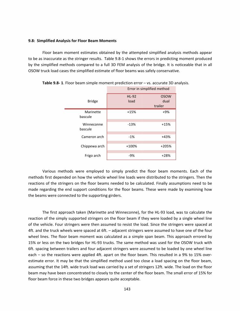
143

9.8: Simplified Analysis for Floor Beam Moments

Floor beam moment estimates obtained by the attempted simplified analysis methods appear

to be as inaccurate as the stringer results. Table 9.8‐1 shows the errors in predicting moment produced

by the simplified methods compared to a full 3D FEM analysis of the bridge. It is noticeable that in all

OSOW truck load cases the simplified estimate of floor beams was safely conservative.

Table 9.8‐ 1. Floor beam simple moment prediction error – vs. accurate 3D analysis.


Bridge

HL‐92load

OSOW dual

trailer

Marinette bascule

+15% +9%

Winneconne bascule

‐13% +15%

Cameron arch ‐1% +43%

Chippewa arch +100% +205%

Frigo arch ‐9% +28%

Various methods were employed to simply predict the floor beam moments. Each of the

methods first depended on how the vehicle wheel line loads were distributed to the stringers. Then the

reactions of the stringers on the floor beams needed to be calculated. Finally assumptions need to be

made regarding the end support conditions for the floor beams. These were made by examining how

the beams were connected to the supporting girders.

The first approach taken (Marinette and Winneconne), for the HL‐93 load, was to calculate the

reaction of the simply supported stringers on the floor beam if they were loaded by a single wheel line

of the vehicle. Four stringers were then assumed to resist the load. Since the stringers were spaced at

4ft. and the truck wheels were spaced at 6ft. – adjacent stringers were assumed to have one of the four

wheel lines. The floor beam moment was calculated as a simple span beam. This approach errored by

15% or less on the two bridges for HL‐93 trucks. The same method was used for the OSOW truck with

6ft. spacing between trailers and four adjacent stringers were assumed to be loaded by one wheel line

each – so the reactions were applied 4ft. apart on the floor beam. This resulted in a 9% to 15% over‐

estimate error. It may be that the simplified method used too close a load spacing on the floor beam,

assuming that the 14ft. wide truck load was carried by a set of stringers 12ft. wide. The load on the floor

beam may have been concentrated to closely to the center of the floor beam. The small error of 15% for

floor beam force in these two bridges appears quite acceptable.

144

A second approach was used in the Cameron bridge because of the different geometry with

7.83ft. stringer spacing. The OSOW loading effects were estimated by first taking the axle and wheel

configuration and placing it transversely near the center of the deck. The portion of load going to each

stringer was calculated by assuming that the slab was a simple span beam strip between stringers. This

provided simple distribution factors for the stringers. When the slabs were loaded, their reactions on

the stringers were easily calculated. Then the reaction from a stringer line on the floor beam was

calculated by applying a full wheel line of the OSOW vehicle on the stringer. Finally the load on the floor

beam was taken as the distribution factor times the wheel line reaction. For the HL‐93 loading, since the

stringer spacing was close to the wheel line spacing, one wheel line was applied per stringer and the

reaction on the floor beam calculated. These reactions were then taken as loads on the floor beam.

With the Cameron bridge the first significant problem in the floor beam analysis was recognized.

While the bridge design insured that the flanges and webs of the floor were secured to the girders,

creating a rigid moment resisting connection, analyzing the beams as if their ends were “fixed” was

unsatisfactory. The negative end moments developed in the simple analysis were far above those found

in the 3D analysis and the positive moments were smaller. It became apparent that a simple analysis

with fixed ends was inappropriate. In the real bridge the tie girder torsional stiffness was insufficient to

completely restrain the floor beam rotation. A pinned end analysis was an improvement, but the error

in positive moment prediction in the girder was +43%.

Comparing the simplified predicted floor beam moment diagram with the moment diagram

from a 3D analysis clearly exhibited the impact of partial composite action that was developed in the

more accurate 3D analysis. Acting compositely with the deck, the composite beam resisted a good

portion of moment through a couple consisting of compression in the deck and axial tension in the floor

beam. The actual moment in the steel floor beam was reduced. A simplified beam analysis was

incapable of capturing this behavior, and overestimated the bending in the steel beam.

Two other modified approaches for floor beam analysis were employed in the Chippewa and

Frigo bridges. HL‐93 analysis was further simplified. Since each of these decks accommodates multiple

HL‐93 lanes, the load on stringers from the trucks HL‐93 truck was assumed to be equally distributed.

With a pin end assumption, even though construction details implied a rigid end joint, the HL‐93

moments were estimated as 100% high and 9% low in the Chippewa and Frigo bridges respectively.

The OSOW truck impact on the Chippewa floor beams was calculated in the same manner as

used for the Cameron bridge. With a pin ended assumption this overestimated the OSOW induced

moment by 205%. The 100% error in HL‐93 estimate and 205% for the OSOW in the Chippewa is

puzzling. A specific source of this error could not be identified.

145

On the Frigo bridge a different approach was taken for the OSOW loading on the floor beam.

The actual stringers were continuous over multiple spans. The wheel line of the OSOW vehicle was

applied to a stringer. To determine the stringer reaction on a floor beam, a simplified 2 span model was

analyzed and the middle reaction calculated. Then the AASHTO distribution factor for the portion of a

wheel line going to a stringer was examined to find a distribution factor of 1.46. A separate analysis

looking at the slab as simply supported, as described above for the Cameron bridge, suggested a higher

factor. An approximate assumption was made – placing 2 wheel lines over the stringer below the middle

of the two trailers, and 1 wheel line on the two adjacent stringers. This provided a moment estimate in

the pin ended floor beam simple model that was 28% higher than the 3D estimate. The 28% difference

could be attributable to the conservative placement of load as if being transferred by only three

stringers.

9.9: Simplified Analysis for Bascule Girder Moments

Moments induced in the girders of the bascule bridges were estimated by placing 2 lanes of HL‐

93 trucks, symmetrically located transversely, and assuming that each of the two bascule girders

resisted one complete truck weight. The bascule girder results are listed in Table 9.9‐1. Predictions for

the HL‐93 loading were accurate – as expected for the simple symmetric loading.

Table 9.9‐ 1. Bascule girder simple moment prediction error – vs. accurate 3D analysis.


Bridge

HL‐92

load

OSOW

dual trailer

Marinette bascule ‐3% +21%

Winneconne bascule +3% +29%

The moments calculated under the OSOW loading were obtained in a slightly different process.

Since the OSOW Dual500‐2 truck and trailer occupied a single lane, assuming that it did not drive down

the middle of the bridge, the truck load was applied in an unsymmetrical pattern. To estimate the

portion of the truck load resisted by a single girder a simple analysis was followed. The truck wheel loads

were applied to a simple supported floor beam and the reaction on the closest girder was calculated as

a portion of the truck axle load. Then that portion of the axle load was applied to the bascule girder at

each axle location, rather than at the floor beam locations. With such loading on the bascule girder the

moment at the support was calculated. The structural model used in this calculation, however, was not

just a cantilever girder. Instead the two girders on opposite leafs were both modelled with fixed ends at

the abutments and a hinge between girder at midspan. The analysis of this indeterminate girder was

146

done using software. While the resulting girder moments were over‐estimated, by 21 to 29%, this

appears to be a simple and conservative method for quick girder analysis.

9.10: Recommended Simplified OSOW Analysis Techniques

Stringers:

No single technique for predicting the moments in stringers was identified. The moment in

stringers on a bascule bride with steel grating could not be safely estimated using the AASHTO

distribution factors because of the unusual spacing of the OSOW vehicle wheels. In the bridges with

concrete decks using the 1996 AASHTO Standard Specifications [9] equation from Section 3.23.2.3.1.5

for a distribution factor for 4 or more stringers supporting a concrete floor provided a conservative

estimate of the stringer moment, 16 to 53% high. Part of the error comes due to the AASHTO equation

being developed for a truck with wheel spacing of 6ft. rather than the close wheel spacing that can exist

in OSW dual trailer vehicles. The inability to more accurately estimate the stringer moment with a

simple analysis also comes from the composite character of the stringer. A closer estimate of the

moment in the stringer could be obtained by using the following steps in bridges with composite decks:

1. Place the wheel line loading of the vehicle on a single stringer model and calculate the

internal moment,

2. Calculate the AASHTO Standard Spec distribution factor for the stringer spacing,

3. Adjust the calculated stringer moment by the distribution factor, and

4. Apply that moment to a composite cross section with steel beam and concrete deck,

then calculate the resultant axial force in the steel beam and the moment in the steel

beam.

Floor Beams

In bridges with close spacing between floor beams the loading on the floor beam depends on

how the stringers carry the truck wheel line loads. With long stringer spans, the portion of the vehicle

line load going to a stringer can be estimated using the AASHTO Standard Specifications distribution

equation. With short stringer spans it is recommended that the load going to stringers be estimated by

assuming that the deck is simply supported, non‐continuous, at each stringer. The truck wheel loads

from one axle line should be applied to the slabs and reaction on the slabs calculated. The reactions

represent the portion of the axle load carried by each girder. Then a representative stringer should be

analyzed with a wheel line loading to determine the support reaction. The loads applied to the floor

beam by the stringers can be taken as the portion of load on a stringer multiplying the calculated

stringer reaction. When these loads are applied to the floor beam the beam moments should be

147

calculated assuming that the beam is pin ended. Using this approach the floor beam moments may be

over‐estimated by 50%

Bascule Girder Moments

The moments in bascule girders can be estimated by analyzing a simple, but indeterminate, 2D

model of a single girder line. The girders line is made up of two girders, each assumed fixed at the

abutments and joined by a pinned connection at the middle bridge joint. The load on each girder can be

estimated by first finding the portion of truck weight carried by the girder. This is estimated by analyzing

a model of the floor beam, simply supported, with one axle of wheel loads applied to find the portion of

the axle weight at a reaction. Then the axle loads of the vehicle are directly applied to the girder but

adjusted in magnitude by the portion of axle weight at the floor beam reaction on the girder. This

approach resulted in over‐estimates of girder moments ranging from 15 to 21%.

148

10. Summary

A prime observation from this study is that very large overload vehicles, with total gross weights

nearly seven times the weight of the basic truck used in bridge design, can be allowed to pass over most

of the complex bridges examined. This may be particularly important for the long span bridges, such as

the La Crosse Cameron Avenue tied arch. The Leo Frigo Memorial bridge over the Fox River in Green Bay

was found to be slightly less robust, but even its truck capacity was not limited by the main structural

elements: the arch and the tie beam. There were no cases, of the set of bridges examined, where

vehicles with gross weight of up to 500,000lbs caused the arches, tie girders or hangers of these bridges

to be overloaded.

The forces developed in the long span bridges by the basic design vehicle, AASHTO HL‐93 trucks

weighing 72,000lbs in each of the design lanes, exceeded those created by the overweight trucks on all

of the bridges examined except for the Frigo Memorial Bridge. It was assumed, however, that when one

of these special highly overweight vehicles crossed a bridge all other truck traffic would be held off the

bridge and the vehicles would be travelling at slow speeds.

As a general conclusion it appears that the bridge stringers, which support the concrete deck,

and the floor beams, which support the stringers, are the critical components that need to be closely

examined when an overload vehicle is crossing a bridge. The stringer force capacity limited the bridge

load capacity in three of the five bridges that were closely examined. The floor beam force capacity

controlled in one.

Two bascule bridges were examined. Under the HL‐93 design truck loading, the bridge capacity

was found to be limited by the stringer strength in one case and the floor beam strength in the second

case. When the large overweight vehicles pass over these bridges, however, the capacity is limited by

the strength of the two main bascule girders that support the entire bridge. These observations may be

deceptive since a close examination of two complex parts of the bascule bridge, the midspan joint

between leafs and the tail beam that prevents the bascule leafs from tipping downward, was not

possible in the scope of this project. Though the joints were modelled, the predicted strain conditions

didn’t match measured values found during truck loading. This indicated that a fine modelling of the

stress flows in the regions of the components would be needed to obtain reliable response values.

These critical parts may deserve a detailed examination to insure that stresses remain within acceptable

limits under heavy truck loading.

An alternate method, based on the empirical data from the load test combined with force

predictions from analysis, did indicate that it is highly likely that the tail beam or tail lock could be

severely overloaded (to nearly twice the yield stress) under both full factored HL‐93 design truck loading

149

and the OSOW truck loading. The tail lock beam is an essential resisting element in a bascule bridge and

needs to be guarded. It appears critical that further investigation of the tail beams on an array of

bascule bridges be undertaken.

A general simplified method for estimating forces in stringers and floor beams was not

satisfactorily achieved for all loadings. The portion of truck wheel loads carried by a stringer can be

estimated by using an AASHTO defined distribution factor (from the AASHTO Standard Specifications)

and the stringer moments calculated for HL‐93 truck loading will be acceptable for most bridges with

standard proportions. When the span to spacing ratio of the stringers exceeds 4, as in the Frigo bridge,

then use of the AASHTO factor may produce results that are 25% conservative.

Stringer moments are not successfully predicted using the same AASHTO distribution factor but

for the wheel loads of the OSOW trucks examined. It is unlikely that the AASHTO factor would work with

any vehicle that has wheel spacing on an axle substantially different from the AASHTO assumed 6ft.

spacing. When OSOW trucks were on the bridges examined, the stringer moments could be

conservatively predicted using an alternate method that overestimated by 16% to 124%. The alternate

method estimates wheel loading on a stringer by considering the bridge deck to act as short simply

supported spans between stringers. Calculated reactions from the deck on the stringers, due to wheel

loads, are used to calculate the stringer moments. This method conservatively estimated stringer

moments in all cases.

Floor beam forces were more difficult to predict than the stringer forces when using a simplified

method. One of the primary difficulties is in accounting for the restraint applied to a floor beam by the

supporting girders. In cases where the joint was by web connection only, the floor beam could be

considered pin ended. When the floor beams were rigidly connected to the girders the assumed

support condition was dubious. A fixed end assumption produced a calculation of negative end

moments much larger than actually existed, and of course smaller positive moments. A pin ended

assumption over‐estimated the magnitude of the positive moments. The calculation process is further

complicated by the assumption made regarding the wheel load distribution to the stringers as discussed

above. Since the stringers apply the load to the floor beams, errors in assumptions regarding stringer

load resistance carry into the floor beam calculations. Results for floor beam moment calculations in the

bascule bridges were acceptable with HL‐93 loading, except in the case of the Chippewa arch bridge.

With OSOW vehicle loading the moments were over estimated by 9% to 43% (except with the Chippewa

bridge), a conservative result that may be acceptable for judging capacity.

A simple method for estimating moments in the main girders of bascule bridges was identified.

The portion of a truck load conducted to any girder was first calculated by applying the truck axle line on

a single simply supported floor beam and solving for the portion of total axle load carried to the floor

beam’s reaction on the girder. Then that portion of the truck load was applied directly on the girder, a

contribution from each axle, and the girder moment calculated. The girder moment calculation,

however, had to be dome using a model where each girder had a fixed end and was joined to the girder

in the opposing leaf by a hinged joint. Existence of an initial small gap in the midspan joint was found to

150

have little effect on peak forces and stress. With a gap of 0.125in. in the Winneconne bridge, the

resulting peak stresses change by only 8%. In bridges with well‐maintained joints the effect of an initial

gap on the member forces can be ignored.

151

REFERENCES

[1] Bae, H. and Oliva, M. (2009), “Bridge analysis and evaluation of effects under overload vehicles.”

Rep. No. CFIRE02‐03, Univ. of Wisconsin, Madison, WI.

[2] AASHTO. (2014). “AASHTO LRFD Bridge Design Specifications, 2014”, 7th Ed., American

Association of State Highway and Transportation Officials, Washington, DC.

[3] Chung, W. and Sotelino, E. (2006), “Three‐dimensional finite element modeling of composite

girder bridges.” Engineering Structures 28 (2006): 63‐71.

[4] Wisconsin Department of Transportation, WisDOT Bridge Manual.

http://wisconsindot.gov/Pages/doing‐bus/eng‐consultants/cnslt‐rsrces/strct/bridge‐

manual.aspx

[5] Computers and Structures, INC. CSI Knowledge Base.

https://wiki.csiamerica.com/display/csibridge/Home

[6] Murphy, J., “PCBridge”, http://joeinmadison.com/sharew/share.htm

[7] QConBridge, Washington State Department of Transportation,

www.wsdot.wa.gov/eesc/bridge/software/index.cfm?fuseaction=software_detail&software

_id=48

[8] Koglin, T. (2003), “Movable Bridge Engineering.” John Wiley & Sons, Inc., Hoboken, New Jersey.

[9] Standard Specifications for Highway Bridges. (1996) American Association of State Highway

[10] Wisconsin Department of Transportation, Highway Structures Information System (HSI).

<https://trust.dot.state.wi.us/hsi>

152

Appendix

Critical Bridge Member Locations

A1: Critical Member Locations in Marinette Bridge

A2: Critical Member Locations in Winneconne Bridge

A3: Critical Member Locations in LaCrosse Cameron Avenue Bridge

A4: Critical Member Locations in Chippewa Memorial Bridge

CFIRE

University of Wisconsin-Madison Department of Civil and Environmental Engineering

1410 Engineering Drive, Room 270 Madison, WI 53706

Phone: 608-263-3175 Fax: 608-263-2512 cfire.wistrans.org

cfire cfire 08-03 - wistrans · cfire 08-03 9. performing ... one rigid frame bridge and two short...

Documents