cfd modelling of chalcopyrite heap leaching · the main contribution of this project is that a new...

CFD Modelling of ChalcopyriteHeap Leaching

a thesis presented for the degree of

Doctor of Philosophy of Imperial College London

and the

Diploma of Imperial College London

by

Liping Cai

September 2016

Department of Earth Science and Engineering

Imperial College London

Abstract

Heap leaching is widely applied to recover metals from ore. The behaviour of the uid

and chemical species inside heaps, which involves many coupled physico-chemical phenom-

ena, are highly variable and complex. Computational Fluid Dynamics (CFD) simulation can

provide an ecient approach to investigate these phenomena and oer guidelines to improve

heap design.

Stagnant zones exist in the packed bed with multiphase ow, however, the conventional

advection-dispersion model (ADE) failed to capture this phenomenon, therefore, the mobile

immobile model (MIM) is employed to model the mass transport and heat transfer instead of

the conventional ADE. For predicting the mineral dissolution in heap leaching, we developed

a new semi-empirical model which is an alternative to the traditional shrinking core model

(SCM), but is more exible in ability to t with various dissolution kinetics proles. The key

assumption of this semi-empirical model is validated, and it is calibrated with experiments

for chalcopyrite leaching.

The software Fluidity, which is an unstructured mesh based nite element/control nite

volume modelling, is further developed to implement the reactive mass transport and heat

transfer simulation for heap leaching. The numerical schemes for multiphase ow models are

control volume nite element method (CVFEM) for spacial discretization and the implicit

pressure explicit saturation algorithm (IMPES) for temporal discretization. The mass trans-

port and heat transfer equations are solved implicitly by using the control volume method.

Before the implementation of various heap leaching simulations, the MIM is validated

by experiments and the liquid-solid phase heat transfer models are veried by method of

I

manufactured solution (MMS). Then the reactive transport model for chalcopyrite leaching,

which includes the semi-empirical model for predictions of mineral dissolution, is validated

by three separate experiments.

Various heap leaching simulations are implemented to analyse the leaching performance

and eciency. Four groups of 1D simulations are implemented to evaluate the eects of

the bacterial activity, the form of the mass transport model, solution temperature, Fe3+

concentrations and solution pH on the leaching system. The large scale 2D simulations for

leaching with a heap of trapezoid shape were implemented to evaluate the eects of oblique

walls on the leaching performance. There dierent wall slopes, which are 30, 45 and 60,

are investigated in the 2D simulations.

The main contribution of this project is that a new semi-empirical model and the mobile

immobile model are developed and integrated into a chalcopyrite leaching simulator, the

simulation results of those models approach to the real physical world better than the con-

ventional models. In conclusion, an improved numerical scheme is provided in this project

to investigate and optimise the process of chalcopyrite leaching for industrial purpose.

II

Originality Declaration

I hereby declare that this work is original research undertaken by me and that no part

of this thesis has been submitted for consideration towards another degree at this or any

other institution, and further, that any work which is not my own has been appropriately

referenced.

Liping Cai

September 2016

Copyright Declaration

The copyright of this thesis rests with the author and is made available under a Creative

Commons Attribution Non-Commercial No Derivatives licence. Researchers are free to copy,

distribute or transmit the thesis on the condition that they attribute it, that they do not use

it for commercial purposes and that they do not alter, transform or build upon it. For any

reuse or redistribution, researchers must make clear to others the licence terms of this work.

III

Acknowledgements

I would like to thank my supervisor Prof Stephen Neethling for accepting as his PhD

student and guiding me throughout my research. He is always patient and willing to support

me with helpful suggestions. I would also like to thank my co-supervisor, Dr Gerard Gorman,

for his supervision. I am really grateful to all of my current and past group mates from

both FFLRG and AMCG groups, I have been receiving lots of help from them in these

years. Particular thanks to Dr Frank Milthaler and Dr Simon Mouradian for sharing their

knowledge and experience in Fluidity and helping me to solve the problems I met when I was

developing code. I really appreciate all of my family members and friends for their numerous

supports and encouragements during my PhD.

IV

Table of Contents

Abstract I

Contents V

List of Figures X

List of Tables XVI

NOMENCLATURE XVIII

1 Introduction 1

1.1 Motivation . . . . . . . . . . . . . . . . . . . . . . . . . . . . . . . . . . . . . 1

1.2 Thesis Outline . . . . . . . . . . . . . . . . . . . . . . . . . . . . . . . . . . . 3

2 Literature Review 6

2.1 Introduction . . . . . . . . . . . . . . . . . . . . . . . . . . . . . . . . . . . . 6

2.2 Scales in Heap Leaching . . . . . . . . . . . . . . . . . . . . . . . . . . . . . 7

2.3 Copper Leaching mechanism . . . . . . . . . . . . . . . . . . . . . . . . . . . 9

2.3.1 Factors Eect Leaching . . . . . . . . . . . . . . . . . . . . . . . . . . 9

Eect of Grain Distribution . . . . . . . . . . . . . . . . . . . . . . . 10

Eect of Particle Size . . . . . . . . . . . . . . . . . . . . . . . . . . 12

Eect of Temperature . . . . . . . . . . . . . . . . . . . . . . . . . . 14

V

Eect of Acid Concentration . . . . . . . . . . . . . . . . . . . . . . . 15

Eect of Ferric Ion . . . . . . . . . . . . . . . . . . . . . . . . . . . . 15

Eect of Redox potential and Iron . . . . . . . . . . . . . . . . . . . 15

2.3.2 Passivation and Hindering Dissolution . . . . . . . . . . . . . . . . . 19

2.3.3 Rate Limiting Steps of Copper Dissolution . . . . . . . . . . . . . . . 22

2.3.4 Kinetics of Mineral Dissolution . . . . . . . . . . . . . . . . . . . . . 23

Avrami Equation for Heterogeneous Reactions . . . . . . . . . . . . . 23

Shrinking Core model (SCM) for Solid-Fluid System . . . . . . . . . 24

Diusion through uid Film Control . . . . . . . . . . . . . . . 27

Mass transport through ash layer control . . . . . . . . . . . . 27

Chemical Reaction control . . . . . . . . . . . . . . . . . . . . 28

Mixed Control . . . . . . . . . . . . . . . . . . . . . . . . . . . 29

2.4 Reactive Transport in Porous Media . . . . . . . . . . . . . . . . . . . . . . 29

2.4.1 Model for Single Porous Pellet with Homogeneous Grain Distribution 30

2.4.2 Model for Multiple Porous Pellets in Porous Bed . . . . . . . . . . . . 32

2.5 Previous Models for Bulk Scale and Heap Scale Leaching . . . . . . . . . . . 34

2.6 The Current State of The Art . . . . . . . . . . . . . . . . . . . . . . . . . . 37

2.7 Conclusion . . . . . . . . . . . . . . . . . . . . . . . . . . . . . . . . . . . . . 39

3 Mathematical Formulation 40

3.1 Multiphase Flow in Porous Media . . . . . . . . . . . . . . . . . . . . . . . . 40

3.1.1 Governing Equations . . . . . . . . . . . . . . . . . . . . . . . . . . . 40

3.1.2 Capillary Pressure . . . . . . . . . . . . . . . . . . . . . . . . . . . . 42

3.1.3 Permeability . . . . . . . . . . . . . . . . . . . . . . . . . . . . . . . . 42

3.2 Mass Transport and Heat Transfer With Mobile- Immobile Model . . . . . . 43

3.2.1 Mass Transport Model . . . . . . . . . . . . . . . . . . . . . . . . . . 43

VI

3.2.2 The Liquid-Solid Heat Transfer Model . . . . . . . . . . . . . . . . . 46

3.2.3 The Parameters of The Mass Transport and Heat Transfer Model . . 47

3.3 Chemistry basis . . . . . . . . . . . . . . . . . . . . . . . . . . . . . . . . . . 50

3.3.1 Reaction of Chalcopyrite Leaching . . . . . . . . . . . . . . . . . . . 50

3.3.2 Bioleaching model . . . . . . . . . . . . . . . . . . . . . . . . . . . . 51

3.3.3 Chemical Reaction Rate Kinetics . . . . . . . . . . . . . . . . . . . . 53

3.4 Basis of The Model . . . . . . . . . . . . . . . . . . . . . . . . . . . . . . . . 55

3.5 Conclusion . . . . . . . . . . . . . . . . . . . . . . . . . . . . . . . . . . . . . 57

4 Analysis of Base Experiment 59

4.1 Experiment Error . . . . . . . . . . . . . . . . . . . . . . . . . . . . . . . . . 61

4.1.1 Copper Extraction and Concentration . . . . . . . . . . . . . . . . . . 61

4.1.2 pH,Eh and Iron Concentration . . . . . . . . . . . . . . . . . . . . . . 64

4.2 Dissolution Kinetic Analysis . . . . . . . . . . . . . . . . . . . . . . . . . . . 65

4.2.1 Analysis with SCM . . . . . . . . . . . . . . . . . . . . . . . . . . . 66

4.2.2 Analysis with Avrami Equation . . . . . . . . . . . . . . . . . . . . . 67

4.3 Conclusion . . . . . . . . . . . . . . . . . . . . . . . . . . . . . . . . . . . . . 69

5 A New Semi-empirical Model for Leaching 71

5.1 Theoretical Basis . . . . . . . . . . . . . . . . . . . . . . . . . . . . . . . . . 71

Grain scale . . . . . . . . . . . . . . . . . . . . . . . . . . . . . . . . 72

Rock scale . . . . . . . . . . . . . . . . . . . . . . . . . . . . . . . . . 73

Bulk scale . . . . . . . . . . . . . . . . . . . . . . . . . . . . . . . . . 73

5.2 Validation of The Separability Assumption . . . . . . . . . . . . . . . . . . . 74

5.3 Calibrating The Model . . . . . . . . . . . . . . . . . . . . . . . . . . . . . . 79

5.4 Conclusion . . . . . . . . . . . . . . . . . . . . . . . . . . . . . . . . . . . . . 80

6 Numerical Scheme and Model Validation 81

VII

6.1 Numerical Framework . . . . . . . . . . . . . . . . . . . . . . . . . . . . . . 81

6.1.1 Multiphase Flow . . . . . . . . . . . . . . . . . . . . . . . . . . . . . 82

Spatial Discretization . . . . . . . . . . . . . . . . . . . . . . . . . . . 82

Time Discretization . . . . . . . . . . . . . . . . . . . . . . . . . . . . 83

6.1.2 Mass Transport and Heat Transfer . . . . . . . . . . . . . . . . . . . 83

Spatial Discretization . . . . . . . . . . . . . . . . . . . . . . . . . . . 84

Time Discretization . . . . . . . . . . . . . . . . . . . . . . . . . . . . 85

6.2 Verication and Validation of Code . . . . . . . . . . . . . . . . . . . . . . . 87

6.2.1 Validation of The Mobile-imobile Model . . . . . . . . . . . . . . . . 87

6.2.2 Validation of Semi-empirical Model . . . . . . . . . . . . . . . . . . . 92

6.2.3 Verication for Two Phase Heat Transfer . . . . . . . . . . . . . . . . 98

6.3 Conclusion . . . . . . . . . . . . . . . . . . . . . . . . . . . . . . . . . . . . . 106

7 1D Simulations and Sensitivity Analysis 107

7.1 Model Description-1D . . . . . . . . . . . . . . . . . . . . . . . . . . . . . . 107

7.2 The Eect of Bacteria . . . . . . . . . . . . . . . . . . . . . . . . . . . . . . 110

7.3 The Eect of MIM . . . . . . . . . . . . . . . . . . . . . . . . . . . . . . . . 117

7.4 Sensitivity Analysis . . . . . . . . . . . . . . . . . . . . . . . . . . . . . . . . 124

7.4.1 The Eect of Solution Temperature . . . . . . . . . . . . . . . . . . . 124

7.4.2 The Eect of Fe3+ and pH . . . . . . . . . . . . . . . . . . . . . . . . 132

7.5 Conclusion . . . . . . . . . . . . . . . . . . . . . . . . . . . . . . . . . . . . . 139

8 Heap Scale 2D Modelling 142

8.1 The Eect of The Heap Wall Slope . . . . . . . . . . . . . . . . . . . . . . . 154

8.2 Conclusion . . . . . . . . . . . . . . . . . . . . . . . . . . . . . . . . . . . . . 159

9 Conclusion and Future Work 160

9.1 Future Work . . . . . . . . . . . . . . . . . . . . . . . . . . . . . . . . . . . . 163

VIII

References 165

Appendix A Experimental Data 180

IX

List of Figures

1.1.1 The illustration of the heap leaching process [113] . . . . . . . . . . . . . . 2

2.3.1 A conceptual 4-stage dissolution model [78] . . . . . . . . . . . . . . . . . . 22

2.3.2 The endothermic reaction of a single solid matrix with gas [141] . . . . . . . 25

2.3.3 The shrinking core models; (a) The dissolution rate is controlled by mass

transport through the uid layer; (b) The dissolution rate is controlled by

mass transport through the ash layer; (c) The dissolution rate is controlled

by chemical reaction rate [89] . . . . . . . . . . . . . . . . . . . . . . . . . . 27

3.2.1 The Axial Dispersion Coecient for Mobile-Immobile Model [70] . . . . . . 49

3.3.1 The growth rate temperature dependence of mesophile versus temperature [85] 52

4.0.1 Micro-CT scan of a single rock, showing the change of extraction of the

mineral grains within a rock. [92] . . . . . . . . . . . . . . . . . . . . . . . . 60

4.1.1 The mean and experimental errors in the Copper concentration and extrac-

tion calculated from K1, the vertical lines indicate the intervals used to cal-

culate the mean and errors. . . . . . . . . . . . . . . . . . . . . . . . . . . . 63

4.1.2 The mean and experiment error of Eh, Fe concentration and Ph calculated

from K1 . . . . . . . . . . . . . . . . . . . . . . . . . . . . . . . . . . . . . . 65

4.2.1 Kinetic analysis with SCM, the solid line is SCM with diusion control, while

the dashed line is SCM with reaction control . . . . . . . . . . . . . . . . . 67

4.2.2 Kinetic analysis of the experiment results with Avrami Equation. . . . . . . 68

X

5.2.1 Optimisation of n′ for the new explicit model over a wide range of κc, with

associated extraction errors . . . . . . . . . . . . . . . . . . . . . . . . . . . 77

5.2.2 Extraction curve for the worst case with κc = 10 . . . . . . . . . . . . . . . 77

5.2.3 The peak errors over a range of non-dimensional external concentrations and

selected intrinsic reaction orders . . . . . . . . . . . . . . . . . . . . . . . . 78

5.3.1 The semi-empirical curve interpolated by cubic spline, dεdt

1κVersus ε, of copper

extraction. . . . . . . . . . . . . . . . . . . . . . . . . . . . . . . . . . . . . 79

6.1.1 The equivalent control volume dual mesh (solid line) constructed on a piece-

wise linear continuous nite element parent mesh (dashed mesh) [5] . . . . . 82

6.1.2 The piecewise constant, element centred shape function of lowest order dis-

continuous Galerkin method [5] . . . . . . . . . . . . . . . . . . . . . . . . . 84

6.2.1 The experimental setup of the tracer test for the immobile-mobile model [70] 88

6.2.2 Comparison of the CFD simulation results for the mobile-immobile model

with the experiment results . . . . . . . . . . . . . . . . . . . . . . . . . . 90

6.2.3 The order of convergence of mobile-immobile model . . . . . . . . . . . . . 91

6.2.4 Comparison of the CFD simulation results for the mobile-immobile model,

conventional advection-dispersion model with the experiment results. . . . . 91

6.2.5 The comparison of simulation and experiment data for copper extraction . . 93

6.2.6 The comparison of simulation and experiment data for copper concentration

in leachate . . . . . . . . . . . . . . . . . . . . . . . . . . . . . . . . . . . . 94

6.2.7 The comparison of simulation and experiment data for redox potential of

leachate . . . . . . . . . . . . . . . . . . . . . . . . . . . . . . . . . . . . . . 95

6.2.8 The comparison of simulation and experiment data for iron concentration in

leachate . . . . . . . . . . . . . . . . . . . . . . . . . . . . . . . . . . . . . . 96

6.2.9 The comparison of simulation and experiment data for pH of leachate . . . 97

6.2.10 The l2-norm of the errors along with various temporal and spatial discretiza-

tions. . . . . . . . . . . . . . . . . . . . . . . . . . . . . . . . . . . . . . . . 101

XI

6.2.11 Convergence analysis for temporal discretization with 800 mesh elements, the

plot of absolute errors for time steps of 2,1,0.5,0.25,0.125 and 0.0625s . . . . 102

6.2.12 Convergence analysis for spatial discretization with ∆t = 0.0625s, the plot of

absolute errors for mesh with 10, 25, 50, 100, 200, 400, 800 elements. . . . . 104

6.2.13 The order of convergence for temporal discretization, with the mesh of 800

elements. . . . . . . . . . . . . . . . . . . . . . . . . . . . . . . . . . . . . . 105

6.2.14 The order of convergence for spatial discretization, with the time step of

0.0625s. . . . . . . . . . . . . . . . . . . . . . . . . . . . . . . . . . . . . . . 106

7.2.1 The comparison between the base model and the bioleaching model; (a)

The average copper extraction of the whole heap; (b) The average copper

concentration in the solutions inside the heap. . . . . . . . . . . . . . . . . . 111

7.2.2 The average heat production of dierent reactions; (a) Base model; (b) Bi-

oleaching model. Note LHS scale is much smaller than RHS. . . . . . . . . 111


Average rock and liquid temperature of the whole heap; (b) Average bacteria

population in the liquid; (c) Average ferric concentration in the heap; (d)

Average ferrous concentration in the heap; (e) Average pH in the heap; (f)

Average copper concentration in the heap. . . . . . . . . . . . . . . . . . . . 112

7.2.4 The variables along the height of heap with time; (a) chalcopyrite extrac-

tion; (b) Heap temperature (average of rock and liquid temperature); (c)

Ferric concentration; (d) Ferrous concentration; (e) Mesophiles population;

(f) Moderate thermophiles population; (g) pH; (h) Jarosite concentration. . 116


The average copper extraction of the whole heap; (b) The average copper

concentration in the solutions inside the heap. . . . . . . . . . . . . . . . . . 118

7.3.2 The comparison between the conventional ADE model and the MIM; (a)

Average rock and liquid temperature of the whole heap; (b) Average ferric

concentration in the heap; (c) Average ferrous concentration in the heap; (d)

Average pH in the heap; (e) Average copper concentration in the heap. . . . 119

XII

7.3.3 The variables along the height of heap with time of the MIM, (the con-

centrations are based on the mean of the mobile and immobile value); (a)

Chalcopyrite extraction; (b) Average copper concentration inside the heap;

(c) Average dierence between the mobile and immobile copper concentra-

tion; (d) Average concentration of jarosite inside the heap; (e) Average pH

inside the heap; (f) The average dierence between the mobile and immobile

pH. . . . . . . . . . . . . . . . . . . . . . . . . . . . . . . . . . . . . . . . . 121

7.3.4 The variables along the height of heap with time of the MIM, (the concentra-

tions are based on the mean of the mobile and immobile value); (a) Average

ferrous concentration inside the heap; (b) Average dierence between the

mobile and immobile ferrous concentration; (c) Average ferric concentration

inside the heap; (d) Average dierence between the mobile and immobile

ferric concentration; (e) Average temperature inside the heap; (f) Average

dierence between the mobile and immobile temperature. . . . . . . . . . . 123

7.4.1 Comparing the models with three dierent solution temperature applied from

heap top; (a) Chalcopyrite extraction; (b) Average copper concentration in

the heap; (c) Average temperature of the heap. . . . . . . . . . . . . . . . . 125

7.4.2 Comparing the models with three dierent temperature; (a) Average pH in

the heap; (b) Average jarosite concentration in the heap. . . . . . . . . . . . 126

7.4.3 Comparing the models with three dierent temperature; (a) Average ferrous

concentration in the heap; (b) Average ferric concentration in the heap; (c)

Average ferrous oxidation rate. . . . . . . . . . . . . . . . . . . . . . . . . . 127

7.4.4 The comparison of the variables between to high temperature and low tem-

perature; (a) Copper extraction; (b) Copper concentration; (c) Heap tem-

perature; (d) pH. . . . . . . . . . . . . . . . . . . . . . . . . . . . . . . . . . 129

7.4.5 The comparison of the variables between to high temperature and low tem-

perature; (a) Ferrous concentration; (b) Ferric concentration; (c) Ferrous

oxidation rate; (d) The concentration of jarosite. . . . . . . . . . . . . . . . 131

XIII

7.4.6 The comparison of the copper extraction; (a) Comparing the copper extrac-

tion of high and low pH/Fe3+ models with the base case; (b) Comparing the

spatial and temporal variation of the copper extraction in the high Fe3+ and

low pH cases. . . . . . . . . . . . . . . . . . . . . . . . . . . . . . . . . . . . 134

7.4.7 The comparison of the ferric concentration; (a) Comparing the average ferric

concentration of high and low pH/Fe3+ models with the base case; (b) Com-

paring the spatial and temporal variation of the ferric concentration in the

high Fe3+ and low pH cases. . . . . . . . . . . . . . . . . . . . . . . . . . . 135

7.4.8 The comparison of the pH; (a) Comparing the average pH of high and low

pH/Fe3+ models with the base case; (b) Comparing the spatial and temporal

variation of the pH in the high Fe3+ and low pH cases. . . . . . . . . . . . . 136

7.4.9 The comparison of the jarosite precipitation; (a) Comparing the average

jarosite concentrations of high and low pH/Fe3+ models with the base case;

(b) Comparing the spatial and temporal variation of the jarosite concentra-

tions in the high Fe3+ and low pH cases. . . . . . . . . . . . . . . . . . . . . 137

7.4.10 The comparison of the heap temperature; (a) Comparing the average heap

temperature of high and low pH/Fe3+ models with the base case; (b) Com-

paring the spatial and temporal variation of the heap temperature in the high

Fe3+ and low pH cases. . . . . . . . . . . . . . . . . . . . . . . . . . . . . . 138

8.0.1 The forced aeration driven from the heap bottom. . . . . . . . . . . . . . . 143

8.0.2 The liquid ow and saturation inside the heap with 45 slope. . . . . . . . . 147

8.0.3 Day 10, the copper extraction and iron concentrations inside the heap with

45 slope. . . . . . . . . . . . . . . . . . . . . . . . . . . . . . . . . . . . . . 148

8.0.4 Day 25, the copper extraction and iron concentrations inside the heap with

45 slope. . . . . . . . . . . . . . . . . . . . . . . . . . . . . . . . . . . . . . 149

8.0.5 Day 231, the copper and pyrite extractions and copper concentration inside

the heap with 45 slope. . . . . . . . . . . . . . . . . . . . . . . . . . . . . . 150

8.0.6 Day 231, The mobile and immobile iron concentrations inside the heap with

45 slope. . . . . . . . . . . . . . . . . . . . . . . . . . . . . . . . . . . . . . 151

XIV

8.0.7 Day 231, the rock, mobile liquid, immobile liquid temperature and total

bacteria population inside the heap with 45 slope. . . . . . . . . . . . . . . 152

8.0.8 Day 231, The liquid pH inside the heap with 45 slope. . . . . . . . . . . . . 153

8.1.1 The liquid saturation inside the heap with 30 and 60 slope on Day 231. . 155

8.1.2 The dynamic Ferric concentrations, pH and liquid temperature inside the

heap with 45 and 60 slope on Day 231. . . . . . . . . . . . . . . . . . . . 156

8.1.3 The chalcopyrite, pyrite extractions and dynamic copper concentrations in-

side the heap with 45 and 60 slope on Day 231. . . . . . . . . . . . . . . . 157

8.1.4 The total extractions of chalcopyrite and pyrite of the heap with 45 and 60

slope. . . . . . . . . . . . . . . . . . . . . . . . . . . . . . . . . . . . . . . . 158

A.0.1 The calculated extraction of chalcopyrite and pyrite of column experiment

K1 from experimental data. . . . . . . . . . . . . . . . . . . . . . . . . . . . 180

A.0.2 The experimental data of the repeated experiments of K1 . . . . . . . . . . 181

XV

List of Tables

2.1 Schematic representation of sub-processes scales in heap leaching [57] . . . . 8

2.2 Factors that aect heap leaching [57] . . . . . . . . . . . . . . . . . . . . . . 10

2.3 The classication of mineral grains according to their accessibility to solutions

[57] . . . . . . . . . . . . . . . . . . . . . . . . . . . . . . . . . . . . . . . . . 11

3.1 Empirically derived rates of chemical reaction, and the heat of reactions. All

concentrations, denoted by square brackets, have units mol/m3. PO2 is the

partial pressure of oxygen, and DO is the molal concentration of dissolved

oxygen. . . . . . . . . . . . . . . . . . . . . . . . . . . . . . . . . . . . . . . 54

3.2 Main mineral species within ore sample from the experiments used for model

developing and calibration. The data is based on volume percentages [93]. . . 57

4.1 Column and Rock Condition . . . . . . . . . . . . . . . . . . . . . . . . . . . 60

4.2 The condition of the column experiments . . . . . . . . . . . . . . . . . . . . 60

4.3 The tted parameters of Equation 4.1.3 for average copper extraction and

average copper concentration . . . . . . . . . . . . . . . . . . . . . . . . . . . 63

4.4 The experiment errors of the column leaching tests, the relative errors from

the means are indicated in parentheses. . . . . . . . . . . . . . . . . . . . . . 64

4.5 The tted parameters against Avrami Equation . . . . . . . . . . . . . . . . 67

6.1 Column and Rock Condition . . . . . . . . . . . . . . . . . . . . . . . . . . . 89

6.2 Simulation Conditions and Parameters . . . . . . . . . . . . . . . . . . . . . 100

XVI

7.1 The Conditions of Base Model and Common Parameters . . . . . . . . . . . 108

7.2 Parameters and Conditions for Bacteria Leaching . . . . . . . . . . . . . . . 109

7.3 The Parameters and their respective values used in the sensitivity study . . 109

8.1 The Conditions of Heap Operations . . . . . . . . . . . . . . . . . . . . . . . 144

8.2 Parameters and Conditions for Bacteria . . . . . . . . . . . . . . . . . . . . . 145

8.3 Initial and Boundary Conditions for solution concentrations, temperature and

partial pressure (ppO2) . . . . . . . . . . . . . . . . . . . . . . . . . . . . . . 146

XVII

NOMENCLATURE

Acronyms

Symbol Description

ADE Advection Dispersion Equation

CFD Computational Fluid Dynamics

IMPES Implicit Pressure Explicit Saturation

MIM Mobile-Immobile Model

MMS Method of Manufactured Solutions

SCM Shrinking Unreacted Core Model

Roman Symbols

Symbol Description Units

D dispersion coecient m2 · s

C concentration mol ·m−3

g gravitational acceleration m · s−2

H enthalpy of reaction KJ ·mol−1

k frequency factor (prefactor) in the Arrhe-

nius equation

s−1

p pressure Pa

XVIII

Q the heat source/sink term from chemical

reaction

Kw ·m−3

R the source/sink term from chemical reaction mol ·m−3 · s−1

r radius of particle m

s saturation -

T temperature K

t time s

z heap length m

K eective permeability m2

u advection velocity m · s−1

v Darcy velocity m · s−1

Greek Symbols


α mass/heat transfer coecient between the

mobile and immobile phase

s−1

κ reaction rate constant mol ·m−2 · s−1

λ thermal diusivity m2 · s−1

µ dynamic viscosity N · s ·m−2

ω weighting constant (a ratio of mo-

bile/immobile mass to the total mass)

-

φ porosity -

Ψ bacteria population attached to ore bacteria · kg ore

ψ bacteria population in solution bacteria ·m−3

ρ density kg ·m−3

XIX

θ the volumetric content of uid -

ε the extraction of mineral -

ϕ rst order growth rate constant s−1

Dimensionless Numbers

Symbol Description Denition

β stoichiometric ratio φbCA0

CB0

κc shrinking core reaction modulus Damkohler II

number

ksr0Cn−1A0 Cm

B0

bDe

τ dimensionless time ttD

C dimensionless reagent concentration CC0

ξ dimensionless particle radius rr0

ξc dimensionless particle core radius rcr0

Ga Galileo number d3pρ2l gφ

3

µ2l (1−φ)3

Pr Prandtl number µlCplλ

Re Reynolds number (characteristic length scale

is the particle diameter)

ulρldpµl

Re∗ Reynolds number (modied by including the

heap porosity)

Rel1−φ

Subscripts

Symbol Description

Xj the X of uid phase j

XA the X of reagent A

Xa the X of air

XB the X of reagent B

XX

Xb the X of bulk solution inside heap

Xim the X of immobile liquid phase

Xi the X of species or bacteria i

Xl the X of liquid phase

Xm the X of mobile liquid phase

Xnw the X of non-wetting phase uid

Xn the X of nth chemical reaction

XT the X of temperature

Xw the X of wetting phase uid

Superscripts

Symbol Description

Xn time step n in Chatper numerical discretization OR the

Xo, Xm order of reaction

Xn+1 time step n+1

Other Symbols


δHt volumetric heat transfer rate between solid

and liquid phases

Kw ·m−3

δHm,im volumetric heat transfer rate between mo-

bile and immobile phases

Kw ·m−3

ηt wetting eciency of trickle bed −

s experimental errors (variance) −

at specic liquid-solid interface m2 ·m−3

XXI

C0 reference concentration mol ·m−3

Cp specic heat capacity KJ ·Kg−1 ·K−1

dp harmonic mean diameter of the particle size m

Eh redox potential mV

Ea activation energy kJ ·mol−1

ht heat transfer coecient between solid and

liquid phases

Kw ·m−2 ·K

k1 rate constant of attachment of bacteria s−1

k2 rate constant of detachment of bacteria s−1

ka absolute permeability -

kr relative permeability m−2

kdeath death rate constant of bacteria s−1

KM Monod parameter kg ·m−3

n′ nonlinear scaling -

pc capillary pressure Pa

pH numeric scale of acidity) −

r0 initial radius of particle m

rc radius of unreacted core of particle m

se eective saturation -

swr residual saturation of wetting phase -

tD characteristic diusion time s

we Lagrangian nite element basis function -

wv control volume basis function -

XXII

Chapter 1

Introduction

1.1 Motivation

For thousands of years, copper has been one of the most important metals that people

have mined. Being one of the most abundant copper-bearing minerals, chalcopyrite (CuFeS2)

accounts for more around 70% of the world's copper population [90]. Approximately 80-85%

of copper is recovered through pyrometallurgical processes, which are the traditional pro-

cesses that consist of concentrating chalcopyrite to a certain grade by otation followed by

smelting [59,90,126]. However, it is not economical to treat low grade ores by these processes

due due to high cost of grinding the material relative to the amount of copper. Alternative

technologies that do not require as much comminution are thus gaining popularity, with heap

leaching being the most widely used alternative [127].

In heap leaching, crushed ore is piled onto large scale heaps with a typical depth of tens

of meters and width of hundreds of meters (see Figure 1.1.1). Leaching solution is then

applied from the top the of heap, and the solution percolates through the rocks, dissolving

metals. After this, valuable metals are recovered from the collected pregnant solutions, via a

process called solvent extraction/electro-winning (SX/EW) [113]. After the copper has been

extracted, the solution is recycled to irrigate the heap. Air is sometimes injected into the

base of heaps, especially in sulphide leaching and is delivered into heap via forced aeration,

which can improve heap bioleaching by promote the bacteria activity [152].

1

Figure 1.1.1: The illustration of the heap leaching process [113]

While chalcopyrite is the most commonly minded copper mineral, it is seldom heap leached

because the leach kinetics are extremely slow with heap leaching being more commonly used

for copper oxides and secondary sulphides [90]. The kinetics and performance of chalcopy-

rite leaching is still not fully understood due to the presence of complex physicochemical

phenomena during leaching. The leach eciency of the system is controlled by various fac-

tors which can be classied into physicochemical parameters, microbiological parameters,

properties of the mineral ore and the processing approaches [21]. All of these factors can

aect the leach kinetics and copper extraction rate. Therefore it is desirable to study the

phenomena behind those factors and thus develop methods and understanding that can be

used to optimise these complex systems.

Developing computational models for chalcopyrite heap leaching is an economical approach

to study and optimize leach kinetics. The main advantages of the computational modelling

is being repeatable, saving time and reducing the need for costly large scale experimental

studies. The modelling of the heap of width and depth of hundreds of meters for years

2

may just take several hours, and the parameters can be adjusted repeatedly to analyse the

trends [103]. By doing computational modelling, dierent leach strategies can be explored to

optimize the heap, while doing heap scale experiment for leach optimization is not practical.

The aim of this project is to develop a numerical model to simulate the reactive mass

transport in chalcopyrite heap leaching. A new semi-empirical model is developed to pro-

vide an alternative to the traditional shrinking core model for leaching modelling. While

various researches have produced heap leach models, this work aims to improve on these by

relaxing some of the assumptions and by incorporating improved sub-models. This model

aims to incorporate a new semi-empirical leach model, the mobile-immobile model for mass

transport, unsteady mixed kinetics of chemical reactions for multiple reactants and bacterial

catalysis into one single model. Finally, the developed model will be applied to realistic heap

leaching simulations for industrial design.

1.2 Thesis Outline

Chapter 2 reviews the copper leaching mechanism and the reactive transport models for

porous systems. The factors that will aect chalcopyrite leaching including mineral grain

distribution in the ores, and particle size and their distributions inside the heap. The eect

of solution concentrations is also reviewed. Also, previous research into the hindering phe-

nomena and rate limiting steps in copper leaching are discussed. The dierent kinetic models

proposed by the previous researchers are also presented in this chapter. The mathematical

formulations and model investigations from previous literature are also discussed.

Chapter 3 presents the mathematical formulations used to simulate the leaching system

in this project. The model is based on and further developed from an open source code,

Fluidity. This model is composed of three main parts, including the multiphase ow model

in porous media which is governed by Darcy's Law, the mass transport and liquid-solid

phase heat transfer model which is formulated in a mobile-immobile approach instead of the

conventional advection dispersion equation, and nally the chemical reaction models which

combine a new semi-empirical model with the existing empirical reaction rate equations to

3

generate the source/sink term in the transport models.

In Chapter 4, the base experiments used to calibrate our models are analysed in detail.

The experimental conditions and data are presented, and the experimental errors for the

copper extraction and dierent species in the solution are calculated in this chapter, which

is used in the later chapter to evaluate the modelling results. Furthermore, the experiment

results are calibrated to the shrinking core model and Avrami equation to determine the rate

controlling steps in the base experiments.

Chapter 5 presents a new semi-empirical model, which can be incorporated into the compu-

tational model to predict the sulphide dissolution rate. This framework directly incorporates

laboratory scale experimental data to predict the heap scale performance, which is compu-

tational ecient and more exible than the traditional shrinking core model in its ability to

t to various dissolution kinetics proles. After the theoretical description, the key model

assumptions are validated.

In Chapter 6, the numerical scheme is described. The model is solved using the control

volume nite element method along with the implicit pressure, explicit saturation algorithm

for the ow model. The route to implement the chemistry model and how the chemical

sources/sinks are coupled with the mobile-immobile model are described in the numerical

discretization part of the transport model. Then, the mobile-immobile model and semi-

empirical model are validated with several experiments, while the two-phase heat transfer

model is veried using the method of manufactured solutions due to a lack of laboratory data.

The sensitivity of the leach performance to various factors are studied in Chapter 7. Sev-

eral 1D simulations are implemented and analysed in detail. In the 1D simulations, the

inuence of the bacterial eect on the ferrous oxidation and the eect of the immobile liquid

on the leaching kinetics are evaluated. The results are compared with a base simulation

which excludes the bacterial eect and is implemented using the conventional advection dis-

persion formulation. Then, the sensitivity analysis of the applied solution concentrations

(pH and Fe3+) and temperature are carried out and they are also compared with the same

base simulation.

4

In chapter 8, the 2D heap scale simulations with traditional trapezoid shapes are im-

plemented and analysed, the simulations are repeated for dierent wall slopes to examine

their eect on the copper extraction. The last Chapter summarizes the main conclusions of

this work as well as providing some thoughts as to the future direction that this work may

take.

5

Chapter 2

Literature Review

2.1 Introduction

The main objective of this study is to model and simulate the phenomena and eciency

of chalcopyrite heap leaching. However, signicant challenges in doing computational mod-

elling have arisen due to the presence of complex physical phenomena that occur during

leaching. These phenomena comprise the coupling of physico-chemical processes within a

multiphase ow inside heaps, such as the transport of solution and air, which is interrelated

with uid-solid reactions, along with the production and transfer of heat energy. The popu-

lation of bacteria, which acts as a catalyst, can also inuence the chemical reactions. These

challenges are particularly signicant inside large heaps with low grade ore [16]. Also, other

external and operational factors can inuence the heap leaching performance, such as the

heap geometry, weather conditions, ore size and shape, etc.

In this chapter, the basic study of hydrometallurgy, especially for the copper industry, is

reviewed. The heap leaching processes can be divided into dierent scales, and those scales

are introduced in Section 2.2. Then, the mechanism of copper leaching are reviewed in detail

in Section 2.3, which focuses on the eects of dierent factors on the chalcopyrite leaching,

and the rate limiting factors for copper dissolution. Then, some well known kinetic models

for reactive solid uid systems, such as shrinking core models and the Avrami equations,

are introduced. Finally, the dierent mass transport models for reactive uid-solid systems,

6

ranging from particle scale models which focuses on an single ore particle to the large scale

models which accounts for the transport in the bulk solution inside packed bed, are reviewed

in Sections 2.4 and 2.5.

2.2 Scales in Heap Leaching

As is illustrated in Table 2.1 [57], the heap leaching processes can be divided into sev-

eral sub-scales, ranging from grain scale, particle scale, meso scale up to macro or heap

scale [39, 57]. The sub-processes within the heap are complex and the interactions between

them are still not clearly understood.

At the scale of the mineral grain, the leaching kinetics are dominated by the chemical

and electrochemical reactions at the grain surface [60]. The chemical reactions are governed

by the temperature and concentrations of reactant, and the dependence of reaction rate on

the temperature are represented by Arrhenius' equation which is characterised by activation

energy [125].

At the particle scale, the topological eect, which refers to the distribution of mineral

grains within a single particle, governs leaching. The leachability of the target minerals is

directly decided by the distribution and accessibility of mineral grains within particles. The

mineralogy of the gangue matrix can also interfere with mineral leaching and biological ac-

tivities in low-grade ores, which can have a signicant eect on leaching eciency [116]. For

example, leaching solution can reach some mineral grains only through the pores and cracks,

the structure of those pores can inuence the leaching rate, and the mineral grains inside

the gangue matrix which are not connected to the pore are not reachable by the solution.

Furthermore, the process of transport of the chemical species to and from the reaction sites

within the particle also plays an important role at the particle level. The size and porosity

of the particle, the diusivity of the reaction species, as well as the diusion gradient are all

important factors within the process [57].

7

Table 2.1: Schematic representation of sub-processes scales in heap leaching [57]

Scale Sub− processes Illustration

Grain scale

(Mineral grain)

Ferric reduction

Mineral oxidation

Sulphur oxidation

Surface processes

Particle scale

(Ore particle)

Topological eects

Intra-particle

diusion

Particle size

distribution

Pure mineral

particle

Particle with

mineral grains

at surface

Porous

particle with

mineral inclu-

sions

Meso scale

(Stagnant cluster)

Gas adsorption

Inter-/ intra-particle

diusion

Microbial growth

Microbial attachment

Microbial oxidation

gas adsorption

inter-particle diusion

intra-particle diusion

attached and oating micro-organisms

Macro scale

(Heap)

Unsaturated solution ow

Gas advection

Water vapour transport

Heat balance

solution ow

internal heat

generation

gas ow

8

At the meso scale of clusters of ore particles, the leaching kinetics are inuenced by the

combined eects of gas and liquid ow, intra- and inter-particle diusion in the stagnant

zones, and oxidation as well as the growth of bacteria. Important processes at this aggregate

level are the dissolution of the oxygen from the air space to the solution phase, and the

diusion of the reactants and reaction products through the inter-particle pores, and the

microbial activity. In heap bioleaching, the crucial reactant is oxygen, since the extent of

the ferrous oxidization by microbes and the reduction of sulphur species are decided by the

availability of oxygen in the system [57].

The largest macro-scale processes are mainly the `ow' processes within the heap, which

are the solution, gas and heat ow through the heap. The kinetics at this level are governed

by the transport of the species and energy into, across, and out of the heap [57].

2.3 Copper Leaching mechanism

The copper leaching chemistry and associated mechanisms are widely studied, and the

complex physico-chemical phenomena have been discussed and argued by various researchers.

In this section, the copper leaching mechanism is reviewed, the factors that will inuence

the leaching mechanism are discussed in Section 2.3.1. Then the controversial phenomena

of passivation and hindering eects, are reviewed in Section 2.3.2. The rate limiting steps

in chalcopyrite leaching are presented in Section 2.3.3, and nally, some kinetic models for

mineral dissolution are reviews in Section 2.3.4.

2.3.1 Factors Eect Leaching

The extent of metal extraction in heap leaching are aected by factors such as environ-

mental conditions, biological and physico-chemical phenomena, which are listed in Table

2.2 [3,47,57,99,126,132]. To make the leaching system function properly, the correct chem-

ical and physical conditions are necessary, which involves reasonable ore particle sizes, the

accessibility of the mineral grains to the solution and oxygen, minimal precipitation to avoid

the blockage of the percolation channels, reduced consumption of acid, etc [37, 112]. Dur-

9

ing the leaching process, the pore structure of the heap continually evolves and varies both

temporally and spatially, since the physical, chemical and biological reactions can cause dis-

solution, deposition and solute transfer. Natural subsidence also occurs under irrigation [77].

Table 2.2: Factors that aect heap leaching [57]

Physical and chemical Biological Mineral properties Processing

Redox potential (Eh) Microbial diversity Mineral type Leaching mode

Temperature Bacteria population

density

Acid consumption Pulp density

pH Spatial distribution

of bacteria

Porosity Heap geometry

Mass Transfer Bacteria activity Surface area etc.

Oxygen availability Metal tolerance Hydrophobicity

Pressure Attachment of

bacteria to

ore particles

Grain size

Presence of inhibitors etc. Formation of

secondary mineral Ferric concentration Galvanic

interactions Water potential etc.

Nutrient availability

carbon dioxide

content Light

surface tension

etc.

Eect of Grain Distribution

The distribution of mineral grains within each ore particles decides their accessibility to

the leaching solution. Five classes of distributions are illustrated in Table 2.3 [57]. The class

(d) and (e) do not contribute to the leaching rate unless new cracks and ssures are created

in the gangue due to the prolonged action of the leaching solution [57]. According to the

particle sizes, the leaching rate can be classied into four regimes [130]:

10

Table 2.3: The classication of mineral grains according to their accessibility to solutions [57]

Classes Illustration

(a) Grain exposed to leach solution at the

surface of particles

(b)Grains exposed to the leach solutions

via pores or cracks

(c) Grain which become exposed to the

leach solutions only after other grains have

reacted

(d) Grain from which pores or ssures that

do not extend to the particle surface depart

(e) Grain located inside the particles and

not connected to pores

Particle size is similar to mineral grains In this case, the leaching rate is compa-

rable to the case of the completely liberated grains, and the inert gangue has little

inuence on the leaching rate. The leaching is under surface reaction control, and the

copper is extracted by a shrinking of the particle during reaction.

Particle size is slightly larger than that of mineral grains Most of the mineral

grains are obstructed by impervious inert gangue, and they can access to the leaching

solution only via the pores and cracks in the inert matrix. In this case, the leaching

is still under surface reaction control, but the diusion starts to aect the rate due to

11

the obstructed access of solution to most of the mineral grain surfaces. In this regime,

the particle size does not play an important role in the dissolution rate

The larger particle sizes than the previous case Although overall leaching mech-

anism is still under surface reaction control, the rate is further reduced. Because some

of the mineral grains are not accessible to leaching solution at the initial leaching stage,

the leaching of the inner grains are hindered by the outer grains as well as the inert

matrix.

The largest particle sizes In this case, the leaching kinetics are under diusion con-

trol or mixed control. The major rate limiting step is the diusion of the reactant in

solution through the gangue, the large ratio between the particle size and grain size

eectively lengthens the travelling distance of the reactants to the mineral grains, and

makes it harder for the solution to penetrate through the pores. The overall leaching

rate is dramatically reduced.

Eect of Particle Size

The reactions in mineral heap leaching are mostly heterogeneous, which means the reac-

tions take place at the boundaries between dierent phases, and the interfacial areas aect

the reaction rate [57]. Models, such as shrinking core models, have been established to relate

particle size to dissolution kinetics [7]. Generally, when the reactions are under control of

diusion through the particles, the reaction kinetics are dependent on the particle sizes. In

this transport control process, the diusion rate is proportional to the inverse square of the

initial ore particle radius, while in the chemical reaction control case, the dissolution rate is

proportional to the inverse of the unleached portion of the particle radius [42].

Generally, the smaller the particle sizes, the faster the leaching kinetics [57, 90], how-

ever, there are a lot of studies where the reaction rate is independent of the particle sizes

[37,45,102,140]. Therefore, the information of particle size distribution alone is not enough,

the mineralogical and elemental distribution within the sizes also play important roles. Dur-

ing leaching, it is also possible to form precipitates on the surface of the surfaces, which will

also aect the leaching rate as it will cover the surface area [57].

12

Eect of Particle Size Distribution (PSD)

The grain size distribution inside a particle and the spatial distribution of the ore frag-

ments are important in design and operation of heap leaching, since they will aect the

solution ow through the heap by changing the permeability, and it can also decide the

degree of mineral exposure [106]. The extractable minerals and even the leaching chemistry

may be a function of the PSD [41]. In many large scale heap models, the average particle

size is used to represent the varying particle sizes and assumes an homogeneous distribution

of the particles inside the bed and an homogeneous distribution of grains inside the particles,

an implicit assumption of most shrinking core models [15, 55]. However, the homogeneous

distributions of the grains and spherical particle geometry are mostly not valid and can cause

signicant errors [57,83]. Gbor and Jia [55] have established a model to couple the Gamma

PSD functions developed by Herbst [61] with the SCM of three dierent rate controlling

systems, and concluded that neglecting the PSD could cause erroneous results in the SCM

when the variation of the size distribution is high.

Eect of Particle Shape

Most of models, such as the shrinking core model, assume the ore fragments are spherical.

As is discussed in a later section (Section 2.3.4), the shrinking core model simplies the

shape ore of ore to be round, and the model assumes that the volume of an ore under disso-

lution will shrink along it's radius, with the reacted fraction of the ore, which is the fraction

has shrunk, being calculated from the volume equation of sphere (Equation 2.3.18). Al-

though assuming a spherical geometry for the ore fragments provides a convenient approach

to model the diusion process mathematically, most of the ore fragments are not spheri-

cal [120]. The fragments are degraded during leaching, and the solid matrix will become

more porous due to the generation of cracks and ssures due to the dissolution of the min-

erals [97, 98] The factor called `leaching enhancement' or `sphericity factor' is incorporated

in the eective diusion term to account for the progressive modication of the geometric

characteristics of the fragments during leaching [22, 97, 98]. The mineral grains within the

fragments are also not spherical, and it is dicult to characterize the eect of the shape of

the individual grains in each fragments [98, 141]. In some previous models a shape factor

13

is added to the kinetic rate equations for each minerals grain to provide a correction [97,120].

Eect of Temperature

The reaction kinetics are usually highly temperature dependent [141]. Generally, high

temperature can increase the reaction rates [16]. At low temperature the dissolution rate

will usually be controlled by the chemical reaction. At higher temperature, the rate will

usually be controlled by the mass transport and a sharp boundary between the leached

region and unreacted core is expected [142]. Copper sulphide leaching involves multiple

highly exothermic sulphide oxidation reactions, and the heat transport becomes crucial in

modelling the leaching process at high temperature [40], because the oxidation reactions in

copper leaching are signicantly dependent on the temperature, and the activities of the

bacteria employed in the copper bioleaching are strongly temperature dependent [40]. The

exothermic sulphide leaching reactions also generate heat. A number of researchers have

established models which include the inuence of heat generation and balance in the various

chemical and biochemical reactions during heap leaching [40,85,123].

By observing the dependence of leaching rate on temperature, the activation energy (Ea) of

the mineral dissolutions can be derived, and the leaching mechanism can be determined [75].

When the leaching is under chemical control, the leaching rate can be increased by increasing

the temperature by a small amount. Otherwise, if the process is under diusion control, the

changing of temperature can only weakly inuence the leaching rate [42]. It is suggested

that chemical reaction control has an apparent value of Ea of over 40 kJ mol−1, otherwise, it

implies a process under diusion control [42].

Cordoba et al. [29] observed a change of temperature inuences the leaching rate signif-

icantly within the temperature range between 35 and 68 C, where the leached copper is

raised from less than 3% to more than 80%, and Ea is derived to be 130.7 kJ mol−1. Similarly,

Sokic et al. [139] found that the leaching rate was signicantly enhanced when the tempera-

ture was raised from 70 to 90 C in 1.5M H2SO4 solution. On the other side, Dreisinger and

Abed [42] found that the eect of temperature on chalcopyrite dissolution in acid chloride

solution is only signicant within the range of 60 to 70 C, and the eect is weak when the

14

temperature is within the range of 70 to 90 C .

Eect of Acid Concentration

The acid concentration plays an important role in chalcopyrite leaching, since it directly

decides the leaching mechanisms and economics [42]. Keeping the pH low can signicantly re-

duce the ferric precipitation and hydrolysis [90]. The most common lixiviant for chalcopyrite

leaching is sulfuric acid (H2SO4), and increasing the H2SO4 concentration can signicantly

improve the leaching rate [2, 8, 65,114,135].

It is suggested that a suitable concentration of H+ is in the range range from 0.1 to

1.0M [42]. Antonijevic and Bogdanovic [7] observed promoted passivation when pH is less

than 0.5, since the competition of between Fe3+ and H+ results in iron decient surfaces, and

this phenomena become more signicant with highly concentrated acid at 3 to 5M. However,

when the acid concentration reaches 6.0M, the copper extraction is improved dramatically, it

is suggested this phenomenon is due to the increased redox potential (Eh ) of H2O2 resulting

from the increasing H+ ion concentration [2].

Eect of Ferric Ion

Ferric ions (Fe3+) is the dominant oxidant in chalcopyrite leaching [90]. It has been ob-

served that the Fe3+ concentration can signicantly impact the leaching rates of chalcopyrite

when the Fe3+ concentration is lower than 100mM [64,75,90]. Below this level, adding Fe3+

gives a positive eects on leaching rate, whist increased Fe3+ concentration has hardly any

inuence on the extraction rate when the concentration is above 100mM [64].

Eect of Redox potential and Iron

The redox potential (Eh) and iron concentration has been conrmed to play an impor-

tant role in chalcopyrite leaching. There are various investigations and discussions of the

15

eects of the ferric and ferrous ions on the leaching rates. Generally, ferric ions are consid-

ered to be the oxidant that eectively oxidises the chalcopyrite via acid solution (Equation

2.3.1), and the role of ferrous ions in dissolution is only as a source of ferric ions via ferrous

oxidation(Equation 2.3.2):

CuFeS2 + 4Fe3+ → Cu2+ + 5Fe2+ + 2S0 (2.3.1)

4Fe2+ + O2 + 4H+ → 4Fe3+ + 2H2O (2.3.2)

Some researchers suggested that ferrous ions will suppress the dissolution of chalcopyrite.

For instance, Dutrizac [45] and Hirato et al. [64] observed that an increase in ferrous sulphate

can reduce the leaching rate of chalcopyrite.

However, recently a number of researchers have discovered that the chalcopyrite oxidation

rate does not always increase with increasing ferric concentration (or equivalently, redox

potential). The optimum leaching rates can be attained only within a narrow range of re-

dox potentials. Kametani and Aoki [74] carried out experiments on chalcopyrite leaching

with sulphuric solution at 90 C, and found that the leaching rate initially increased with

increasing potential, while the rate decreased suddenly at a critical potential of about 0.45

V (SCE). Sandstrom et al. [133] suggested that the leaching rate was signicantly higher at

a low potential of 0.42 V compared with the high potential of 0.6 V (Ag, AgCl) for both

chemical leaching and bioleaching in sulphuric acid media. Passivation by jarosite precipi-

tation was observed at high redox potential.

Koleini et al. [80] also suggested that the redox potential plays an important role in leach-

ing rates, with the chalcopyrite oxidation preferring a narrow range of potentials around

0.41-0.440 V (Ag, AgCl). Cordoba et al. [28, 29] reported strong evidence that high redox

potential can promote jarosite precipitation. The critical potential they found is 0.45 V (Ag,

AgCl). Nicol et al. [110] suggested that the chalcopyrite dissolution is enhanced within the

potential window between 0.56 and 0.6 V (SHE) in chloride acid solution.

Hiroyoshi et al. [66] found that in sulphate solution high ferrous ion concentration is

benecial to chalcopyrite leaching, the extraction is greater in higher ferrous/ferric ratio

16

region and lower potential region. Furthermore, the authors observed that the addition of

cupric ions together with ferrous ions can enhance the leaching more than ferrous ions alone,

which can not be explained by Equation 2.3.1. To interpret this phenomenon, they proposed

a two-step model:

CuFeS2 + 3Cu2+ + 3Fe2+ → 2Cu2S + 4Fe3+ (2.3.3)

2Cu2S + 8Fe3+ → 4Cu2+ + S + 8Fe2+ (2.3.4)

The chalcopyrite is dissolved to form the intermediate Cu2S, which is more reactive than

chalcopyrite, in the solution with enough Cu2+ ions and Fe2+ ions (and hence low potential).

The Cu2S is further oxidized by Fe3+, and the summing of Equation 2.3.3 and Equation

2.3.4 form the overall reaction of Equation 2.3.1. However, it was suggested based on these

equations that the ferrous ion will suppress the leaching rate if the Cu2+ concentration is

not high enough, hence Hiroyoshi et al. [66] concluded that the active redox potential (Eact)

for oxidative reaction of chalcopyrite under the conditions of 25C and 1atm follows the laws

below:

Ec > Eact > Eox (2.3.5)

Ec = 0.681 + 0.059log(aCu2+)0.75

(aFe2+)0.25(2.3.6)

Eox = 0.561 + 0.059log(aCu2+)0.5 (2.3.7)

where Ec is the critical potential to form Cu2S, Eox is the oxidation potential of Cu2S, and

a i is the activity of species i.

Later, Hiroyoshi et al. [67] dened a new parameter which is the normalized redox potential

Enor of Equation 2.3.8:

Enor ≡E − EoxEc − Eox

' 0.07 + 0.059log[Fe3+]− 0.059log[Fe2+]− 0.03log[Cu2+]

0.12 + 0.015log[Cu2+]− 0.015log[Fe2+](2.3.8)

17

They found that the copper extraction rate versus Enor is independent of the leaching

environment such as the solution compositions, bacteria , solid/liquid ratio. A fast leaching

rate is obtained when the normalized potential is within the range of 0 to 1. When Enor > 1

(E > Ec) the reaction is slow because the intermediate Cu2S is not formed, and the region

where the normalized potential is larger than 1 is the `passive region'. When Enor < 0

(E < Eox), the dissolution stops because Cu2S is not oxidised. The optimum of Enor to

achieve the maximum leaching rate is found to be 0.43, and the functions for the optimum

redox potential is derived to be dependent on the Cu2+ ions and Fe2+ ions concentrations of

Equation 2.3.9:

Eop = 0.652 + 0.036log[Cu2+]− 0.006log[Fe2+] (2.3.9)

Where [i] is the molarity of species i.

Sandstrom et al. [133] agreed with the suggestions of Hiroyoshi et al. [66] because they

also observed an increase in extraction with increasing copper concentration at low poten-

tials. However, Cordoba [30] opposed the proposal from Hiroyoshi et al. [66]. By producing

X-ray diractograms they pointed out that the chalcopyrite is dissolved via the formation

of an intermediate covellite, CuS rather than chalcocite, Cu2S. Then they proposed a new

two-step dissolution equations (Equation 2.3.10 and Equation 2.3.11) to describe the chal-

copyrite oxidation by ferric, which diers from the one suggested by Hiroyoshi et al. [66]:

CuFeS2 + 2Fe3+ → CuS + 3Fe2+ + S0 (2.3.10)

CuS + 2Fe3+ → Cu2+ + S0 + 2Fe2+ (2.3.11)

This suggestion is supported by the observations from Kametani and Aoki [74] that CuS

was found in the residues of chalcopyrite leaching under low redox potential (0.33 V (SCE)).

Nicol et al. [110] also questioned the suggestion from Hiroyoshi et al. [66], as they claimed

that the Equation 2.3.3 is unlikely to occur at potentials above 0.5 V (SHE). There is lack

of experimental evidence to support that the cahlcopyrite is reduced to form chalcocite at

higher potentials. Cordoba [30] further concluded that the Ferric/Ferrous sulphate leaching

18

solution tend to approach an equilibrium with a critical potential of 0.45 V (Ag, AgCl).

A high initial potential will promote jarosite precipitation reducing the solution potential

towards the critical value.

For bioleaching, Yang [158] concluded that the solution redox potential is more inuential

than the bacteria concentration and activity, and more chalcopyrite was dissolved at lower

potential values. The observations supported the conclusions drawn from Cordoba [30] that

more jarosite accumulated with higher initial redox potentials. Similarly, Third et al. [143]

declared that the Eh is far more crucial than the amount and activity of bacterial cells,

although the bacteria are essential to regenerate oxidant for continuing leaching. They sug-

gested that excessive bacterial ferric ion oxidation, and hence a resultant high Eh, can inhibit

the leaching. Therefore only a limited bacterial activity, which produce the ferric ions at a

rate that meets the consumption by the ore, can favour the chalcopyrite leaching. In addi-

tion, Yu [159] claimed that the jarosite precipitation is not important for bioleaching as long

as the redox potential is lower than 0.65 V (SHE), while increasing ferric ion concentration,

and hence Eh, will slow down the dissolution rates.

2.3.2 Passivation and Hindering Dissolution

The dissolution of chalcopyrite is initially fast but soon declines. There has been a lot

of debate among researchers as to the reason for this phenomenon. It has been suggested

that during chalcopyrite dissolution, the formation of surface lms can lead to the hinder-

ing of the dissolution rate, which is referred to as `passivation' for abiotic or biochemical

chalcopyrite heap leaching [58, 78, 94], though the verication of the exact candidates and

mechanisms of passivation is still a controversial topic. Generally, among the various `pas-

sivation' candidates which can hinder the leaching rate, the following four are of the most

concern: metal-decient sulphides, polysulphides (XSn), elemental sulphur (S0) and jarosite

(XFe3(SO4)2(OH)6) [78].

Fu et al. [51] evaluated the passivation candidates for the bioleaching of copper sulphide

minerals, including chalcopyrite, by using A.Ferrooxidans as the leach organism. In their

19

work they conrmed that the passivation layers for chalcopyrite bioleaching consist of copper-

decient sulphide Cu4S11, elemental sulphur S0, and copper-rich iron decient polysulphide

Cu4Fe2S9, while jarosite was not observed on the surfaces and thus may not be responsible

for hindering the dissolution rate. They concluded that the hindering ability of these surface

lms is Cu4Fe2S9 > Cu4S11 > S0 > jarosite. Similarly, by doing various spectroscopic exper-

iments, some researchers have identied that the metal decient sulphides, including poly-

sulphides, are produced during both chemical leaching and bacterial leaching [59,84,95,105].

In addition, a number of researchers claim that jarosite and elemental sulphur do not play

an important role in passivation, but the metal decient sulphides and/or polysulphides pas-

sivate the rate of chalcopyrte oxidation [25,58,95,101,118,157,158].

In contrast, there are some researchers who support the standpoint that jarosite and sul-

phur are to be blamed for the passivation. Some researchers suggested that the jarosite

precipitation formed on the chalcopyrite surface due to the high concentrations of ferric iron

and sulphates will raise the diusional constraint, hence reducing the chalcopyrite dissolu-

tion rate [17, 68]. Parker et al. [117] investigated the oxidative acid leaching of copper and

iron from chalcopyrite under both abiotic and microbial conditions. They concluded that

the disulphide forms quickly on the dissolving chacopyrite surfaces, and the oxidation of the

disulphide phase likely leads to the formation of thiosulphate intermediates, and the further

oxidation of thiosulphate results in a ferric sulphate which is similar to jarisite, they claimed

that this sulphate is a precursor to the nal jarosite precipitation, which is the key to the

hindered dissolution in the chalcopyrite system.

Furthermore, Dutrizac [46] concluded that about 90% of the elemental sulphur formed by

the chalcopyrite dissolution can not be dissolved during chemical leaching of chalcopyrite

with ferric sulphate, and thus will precipitate around the ore. It was observed that the

chalcopyrite grains are enveloped by the sulphur, and the sulphur layers were progressively

growing during leaching, hence the dissolution is passivated. Klauber et al. [79] also drew the

conclusion that elemental sulphur is the major candidate for initial inhibition of chalcopyrite

with ferrous leaching, as elemental sulphur were found to be the primary surface species pro-

duced in their acid ferric leach. However, in bioleaching sulphur-oxidizing microorganisms

can reduce the elemental sulphur passivation, as well as lowering the pH [29,78], and so the

20

diusion barrier caused by S0 is avoided. Nevertheless, Pradhan et al. [126] mentioned that

the elemental sulphur and jarosite coating may inhibit the transport of bacteria, oxidants to

and from the chalcopyrite surface, and further reduce the chalcopyrite dissolution rate.

Moreover, the passivation caused by metal decient sulphides are strongly argued. Mikhlin

et al. [105] conducted experiments to investigate the spectroscopic and electrochemical char-

acterisation of the surface layers of chalcopyrite dissolved in acidic solution. The results

showed that metal decient layers were formed up to several micrometer thick, but it was

observed that the electronic structure of this layer was similar to that of chalcopyrite, and

the results indicated that this layer can hardly hinder the chalcopyrite dissolution. Similarly,

Acero et al. [1] observed an iron-decient surface layer in their chalcopyrite leaching experi-

ment with both sulphuric and hydrochloric acid, but no inhibition eect was found with this

layer.

Furthermore, Klauber [78] questioned the metal-decient sulphide being a hindered disso-

lution candidate as the physical reality of this layer still remained to be examined, and there

is a lack of consistent evidence. For instance, the author argued against the validity of the

demonstration given by Hackl et al. (1995) [58], which indicated an iron decient sulphide

phase is formed and acts as a passiviation layer in chalcopyrite dissolution. Also, it was

discussed that the investigation provided by Buckley and Woods (1984) [25] and Parker et

al. (1981) are not clear-cut, and that the proposal of metal decient sulphide/polysulphide

lm is speculative [78].

In addition to metal decient sulphides, Kaluber et al. [79] and Parker et al. [117] declared

that the polysulphides are also not responsible for the hindering dissolution. The extremely

reactive nature of polysulphide compounds can hardly allow them to form any surface layer

capable of inhibiting the chalcopyrite dissolution, since they are easily oxidized to elemental

sulphur with air, especially with moisture [79,81,117].

21

2.3.3 Rate Limiting Steps of Copper Dissolution

Generally, three types of copper extraction curves are observed: (i) parabolic with time,

(ii) linear with time or (iii) parabolic in the initial stage and followed by linear [78]. The

parabolic kinetics of the copper extraction indicate the chalcopyrite dissolution is hindered

and the rate becomes very slow [108]. Some researchers deduced that this hindered parabola

suggests that the dissolution rate is under the control of the transport of ions and electrons

through the dense sulphur layer [12,14,44,108]. In this parabolic stage, the activation energy

for chalcopyrite dissolution is reported to be between 38 to 83 kJ mol−1 [64]. On the hand,

the linear kinetics suggest the dissolution is under surface reaction control rather than diu-

sion control, the slow chemical reactions with high activation energy are the limiting steps

of chalcopyrite leaching [30,64,72]. The very high activation energy of chalcopyrite leaching

with this linear behaviour was found to be 130.7 kJ mol−1 by Cordoba [30].

To explain the chalcopyrite dissolution steps, Klaubler [78] presented a conceptual 4-stage

dissolution model, which can logically tie together all the experimental observations dis-

cussed previously into one model, the model is illustrated in Figure 2.3.1:

Figure 2.3.1: A conceptual 4-stage dissolution model [78]

Stage 1: The chalcopyrite surface is clear and fresh, and the initial reaction rate is fast

with a low activation energy Ea.

22

Stage 2: The dense layer of elemental sulphur forms on the chalcopyrite surface, which

hinders the dissolution rate and electron transport, hence causes a parabolic rate curve with

a high Ea, if the thick sulphur layer does not peel away, the parabolic behaviour continues.

Stage 3: The peeling of the thick sulphur layer favours the leaching rate, the reaction

is fast with a high Ea, and the leaching curve exhibits a linear behaviour. If the jarosite

formation is precluded by iron and pH control the linear behaviour continues.

Stage 4: If pH and iron is not under control, jarosite precipitation may occur, if this

coats the chalcopyrite surface the parabolic rate curve reappears due to the inhibited mass

transport and/or reduced surface area.

Furthermore, stage 1 alone or stage 1 and 2 together can be treated as the induction

period, while the appearance of stage 3 and 4 depends on the solution conditions, especially

Fe3+, pH and temperature [78].

2.3.4 Kinetics of Mineral Dissolution

The previous section discussed the dissolution rate limits occurring on chalcopyrite surface,

but in reality, the sulphides minerals are only a small fraction of the ore and the leaching

will also be strongly inuenced by mass transport through the ore particle. The apparent

kinetics are thus a combination of mineral surface kinetics and mass transport in the ore

particle. A number of models have been proposed to model these eects, which are used in

a wide range of applications in many uid-solid reactive system rather than just leaching.

Avrami Equation for Heterogeneous Reactions

The reactions in chalcopyrite leaching are heterogeneous, since the reactants are in mul-

tiple phases, and with growing product layers during dissolution. A wide range of mineral

23

reactions with isothermal kinetics can be described using the following empirical form [128]:

dε

dt= kntn−1(1− ε) (2.3.12)

and by separating the variables along with integrating, and incorporating the term 1/n

into the rate constant k, gives the Avrami equation, Equation 2.3.13:

ε = 1− exp(−kt)n (2.3.13)

where k is a rate constant and has the dimension of time−1, t is time and ε is the extraction,

n is a constant that depends on the reaction mechanism. For diusion controlled dissolution,

n trends to be near 0.5, while for chemical reaction controlled dissolution, n ∼ 1.0 [128,139].

To calculate the values of k and n, the following form is generally used to linearize Equation

2.3.13:

ln [−ln (1− ε)] = n lnk + n ln t (2.3.14)

Plotting the Avrami equation in the form of Equation 2.3.14 gives the linear line of

ln [−ln (1− ε)] against ln t, and the value of n, which is the slope of the plotted straight

line. The value of n can be used as an empirical parameter to check the mechanisms of

mineral dissolutions [128].

Shrinking Core model (SCM) for Solid-Fluid System

The simple idealized models called the shrinking unreacted-core models (SCM) were rst

derived by Yagi and Kunii [155], and are the most commonly used model for non-catalytic

uid-solid reactions of particles with unchanged size [55,89,141], The models have been stud-

ied and extended by Szekely [141] and Levenspiel [89]. The porous rock fragments are mostly

considered to be made up of solid grains which will react with the reagent [149]. Based on the

SCM, the models for reactive transport through a single porous fragment have been further

extended and developed, such as the narrow reaction zone model [9], modied unreacted

core shrinking model [115] and the generalized grain model [141] for the negligible diusion

resistance within the individual grains inside the fragments, the modied generalized grain

model [141] and spherical xed packed-bed model [115] for including the diusion resistance

24

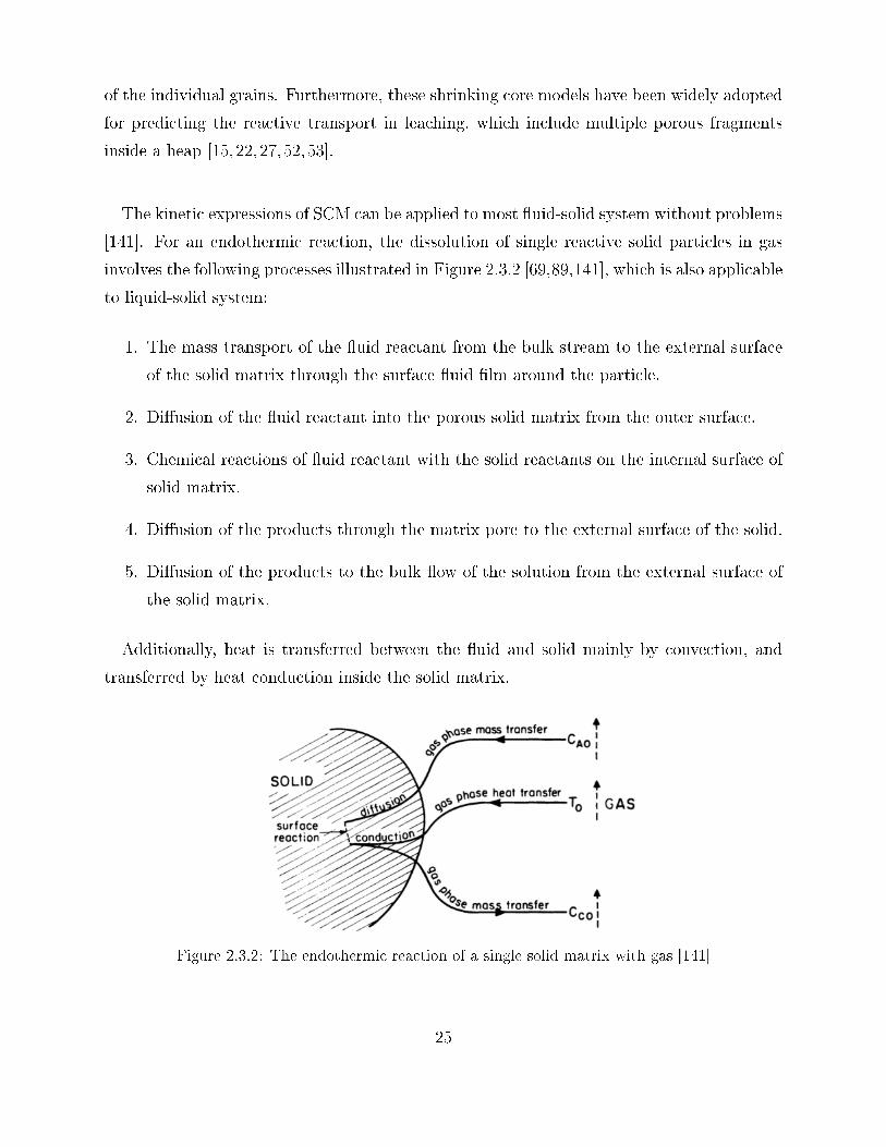
of the individual grains. Furthermore, these shrinking core models have been widely adopted

for predicting the reactive transport in leaching, which include multiple porous fragments

inside a heap [15,22,27,52,53].

The kinetic expressions of SCM can be applied to most uid-solid system without problems

[141]. For an endothermic reaction, the dissolution of single reactive solid particles in gas

involves the following processes illustrated in Figure 2.3.2 [69,89,141], which is also applicable

to liquid-solid system:

1. The mass transport of the uid reactant from the bulk stream to the external surface

of the solid matrix through the surface uid lm around the particle.

2. Diusion of the uid reactant into the porous solid matrix from the outer surface.

3. Chemical reactions of uid reactant with the solid reactants on the internal surface of

solid matrix.

4. Diusion of the products through the matrix pore to the external surface of the solid.

5. Diusion of the products to the bulk ow of the solution from the external surface of

the solid matrix.

Additionally, heat is transferred between the uid and solid mainly by convection, and

transferred by heat conduction inside the solid matrix.

Figure 2.3.2: The endothermic reaction of a single solid matrix with gas [141]

25

In the shrinking unreacted core model (SCM), it is assumed that the uid-solid reac-

tion takes place by surface reaction, the uid and reaction move into the particle with the

completely reacted solids, which are sometimes refer to as `ash' due to the origins of this

model in simulating combustion, behind the reacting surface [89]. If we consider the reaction

described in Equation 2.3.15:

A(fluid) + b B(solid)→ c C + d D (2.3.15)

A pseudo-steady state assumption is made for mass transport, which means that the eect

of accumulation is assumed to be negligible. The uid reactants supplied to the particle are

assumed to be consumed completely by the solid, the change in the volume and radius of

the particle can be related to the variation in the amount of reactant B in the solid [89]:

− dNB

= −b dNA

= −(1− φ)ρBdV = −4π(1− φ)ρ

Br2cdrc (2.3.16)

where φ is the porosity of the particle, ρBis the molar density of the reactant B in pore

free solid, V is the volume of the unreacted spherical particle, b is the stoichiometric factor,

rc is the radius of the unreacted core, NAand N

Bare the amounts of reactant of A and

B. Thus, the relationship between the mass transfer of the reactants and the conversion of

solids is [141]:

b QA

=1

Ap

dNB

dt=VpAp

(1− φ)ρB

dε

dt(2.3.17)

where QAis the ux of reactant A from uid to solid, Ap and Vp are the exterior surface

area and the total volume of the particle respectively, ε is the fraction of the solid reacted,

which is:

ε = 1− (rcR

)3 (2.3.18)

where R is the initial radius of the particle.

According to the resistances of the dierent steps during dissolution, the highest resis-

tance is considered to control the overall dissolution rate. Generally, four dierent kinds of

rate-controlling models are used to approximate the dissolution in uid-solid reactions. By

assuming the particles are spherical, the following four kinetic models are discussed from

Levenspiel and Szekely [89,141].

26

(a) (b) (c)

Figure 2.3.3: The shrinking core models; (a) The dissolution rate is controlled by mass transport

through the uid layer; (b) The dissolution rate is controlled by mass transport through the ash

layer; (c) The dissolution rate is controlled by chemical reaction rate [89]

Diusion through uid Film Control As is illustrated in Figure 2.3.3(a), it is assumed

that there is no reactant at the particle surface for the irreversible reaction under diusion

through the uid layer control. The concentration of reactant in the uid drops from the

bulk value to zero through the layer, thus the concentration driving force is the bulk uid

concentration CAg at the external surface of the uid lm, and the equations for the mass

transfer of the reactants become:

− 1

Ap

dNB

dt= − b

Ap

dNA

dt= b hgCAg (2.3.19)

where hg is the mass transfer coecient between uid and particle.

By combing the Equation 2.3.19 and 2.3.16 and integrating, the time for complete con-

version of the solid reactant at rc=0 is [89]:

tε=1 =(1− φ)ρ

BR

3b kg CAg

(2.3.20)

Then the conversion function, which is the function of extraction and time, for the mass

transport through uid lm control is:

g(ε) =t

tε=1

= εB

(2.3.21)

Mass transport through ash layer control The partially reacted shrinking core particle

under diusion through ash layer control is illustrated in Figure 2.3.3(b). In this system,

27

the uid reactant A is considered to be moving inward with the boundary of the unreacted

core and forming the concentration gradient through the ash layer, but the shrinkage of the

unreacted boundary is much slower than the diusion of A. Under this assumption, it is

reasonable to ignore the movement of the unreacted core at any instant in considering the

diusion along the concentration gradient, and this is the pseudo-steady state approximation

for the mass transport through the ash layer [9]. Then, the reaction rate can be simplied

to be equal to the diusion rate within the ash layer, which can be expressed by Fick's Law:

− 1

4πr2

dNA

dt= Q

A= D

AeffdC

A

dr(2.3.22)

By integrating Equation 2.3.22 across the ash layer with the concentration gradient from

CAg at the external surface of the particle to 0 at the unreacted core, and replacing dN

A

with drc from Equation 2.3.16, the conversion function for diusion through the ash layer

control is derived [89]:

g(ε) =t

tε=1

= 1− 3(1− εB

)2/3 + 2(1− εB

) (2.3.23)

The time for the complete conversion is:

tε=1 =(1− φ)ρ

BR2

6b DAeff CAg

(2.3.24)

Chemical Reaction control The reaction under chemical reaction control is illustrated

in Figure 2.3.3(c). The dissolution rate is controlled by surface reaction around the unreated

boundary and without the diusion resistance across the ash layer, thus the concentration of

the reactants at the reaction surface are the same as the concentration of the bulk uid [141].

The ux of the species is equal to the consumption of the reactant by surface reaction at the

unreacted core:

− 1

4πr2c

dNB

dt= − b

4πr2c

dNA

dt= b k1 CAg (2.3.25)

where k1 is the rst order rate constant for surface reaction. By integrating Equation 2.3.25,

the conversion function for chemical reaction control is [89]:

g(ε) =t

tε=1

= 1− (1− εB

)1/3 (2.3.26)

The time to complete the conversion is:

tε=1 =(1− φ)ρ

BR

b k1 CAg

(2.3.27)

28

Mixed Control Throughout the conversion progresses, the relative eect of dierent resis-

tances vary, and it might not be appropriate to assume that the dissolution is under a single

control [89]. Under the simultaneous eects from the above resistances and based on the

pseudo-steady state assumption, the time to achieve a certain conversion is approximately

the sum of the time required to reach the same conversion by each single resistance control,

and at any instant the conversion rate can be expressed by the function of the combination

of the individual resistance [89,141]:

− 1

4πR2

dNB

dt=

b CA

1kg

+ R(R−rc)rc Deff

+ R2

r2c k1

(2.3.28)

The above Equation 2.3.28 can be approximated to the following simplied equation:

ttotal ' tfilmalone + tash alone + treaction alone (2.3.29)

2.4 Reactive Transport in Porous Media

The important structural feature of most shrinking core models applied to ore-leaching

is that the sub-particles (grains) of minerals are considered to be distributed throughout

the porous particles along with the inert material. The liquid reactants diuse into the

solution-lled channels which surround the grains and react with them [10,122,149]. In the

general case of a porous solid, the sharp boundary between the reacted and unreacted zone

which is described in the shrinking core models in Section 2.3.4 will not occur. Instead the

degree of conversion will change gradually throughout the particles and a partially reacted

zone exists between the completely reacted zone and the unreacted zone [141]. Thus, the

following diusion equations are presented to formulate the reactive transport in porous ore.

For quasi-spherical rocks, the mass transport through the pores of a solid matrix can be

described by the diusion equation for spheres [9]:

θi∂Cj∂t

= Djeff [∂2Cj∂r2

+ (2

r)(∂Cj∂r

)] +Rj (2.4.1)

29

where Cj is the concentration of dissolved solute j in the phase i inside the rock pores, r is

the distance along the radius of the rock. The eective diusion coecient Djeff is dened

by:

Djeff =θiDoi

τ(2.4.2)

where Doi is the diusion coecient for species j in a clear uid i, and τ is the tortuosity,

which accounts for the increased tortuous path. The tortuosity is the actual ow length

divided by the straight path length in clear uid [49,134,137].

Multiple solid reactants exist inside the inert porous solid in many real leaching systems

and the competition between those reactants can eect the dissolution rate [41]. The indi-

vidual kinetics equations for dierent mineral species are discussed by Bradley et al. and

Madsen et al [98,120] to calculate the consumption and generation rate Rj of the species by

chemical reactions in Equation 2.4.1.

The following grain models which assume an homogeneously distribution of the mineral

grains throughout the ores, are generally proposed to model the dissolution process of the

porous solids [9,115,141]. These can normally be reduced to two cases, including or exclud-

ing the diusion resistances of grains.

2.4.1 Model for Single Porous Pellet with Homogeneous Grain Dis-

tribution

There are models in the literature which can describe the leaching system of the particle

scale. As has been mentioned before, mineral grains are distributed throughout each single

ore, and in the following models the mineral grain distribution are simplied to be homoge-

neous. They are also based on the assumption that both fragments and grains are spherical.

In these models the shrinking core description can be applied at both the scale of the particle,

as well as at the scale of the individual grains. Two cases of increasing complexity can thus

be considered.

30

Negligible Intragranular Diusion Resistance of Individual Grains

Under the assumption that the diusion resistances of the product layer of individual

grains are neglected, the mathematical model is simplied to include only the eect of

intrinsic chemical kinetics and the mass transport of species through the pore-solution of the

fragments [115, 141]. If the diusion resistance throughout the pellet is negligible and the

chemical reaction controls the overall leaching rate, then the concentration of the solution

is assumed to be uniform throughout the pellet, and the shrinking core models discussed in

Section 2.3.4 can be applied directly to every individual grain without transport resistances,

and the fragment is considered to be the agglomerate of the those grains which are reacting

simultaneously [141]. If the mass transport of the reactants in the pore-solution controls

the leaching and without chemical reaction limitation, then the shrinking core models of

diusion control discussed in Section 2.3.4 can be directly applied to the pellet [141].

In most reactions of the porous solid, the leaching process is controlled by mixed kinetics

and the sharp discontinuous boundary of the unreacted core will usually not exist. Instead

the reaction will take place in a reaction zone with progressively reacted mineral grains

[10, 115]. Moreover, the reaction rates during leaching will also depend on the degree of

conversion of the individual grains, since the surface area available for the reaction is changing

[141]. Under the pseudo-steady state assumption and neglecting external mass transfer

resistance of the pellet, the mass transport of the species within the porous pellet is simplied

to [10,138]:

0 = DAeff∇2C

A−R

A(2.4.3)

where CAis the uid reactant concentration in a unit volume of pellet, and R

Ais the local

rate of consumption per unit volume of pellet, which depends on the position in the pellet.

The local consumption rate is dependent on the local reaction rate and the local conversion of

the grains. Under rst order reaction kinetics and assuming spherical grains, the relationship

is [138]:

RA

= (1− ε)k1CA

3r2cg

r30g

(2.4.4)

where rcg is the radius of the unreacted core of the individual grain, and r0g is the initial

radius of the grain.

Within each individual grain, the local reaction rate can be expressed by the model of

31

chemical reaction control [138]:

(1− ε)ρB

drcgdt

= bk1CA(2.4.5)

Including Intragranular Diusion Resistance of Individual Grains

If the assumption of negligible diusion resistance within the mineral grain is not valid,

then the intragranular diusion resistance should be included in the model. Papanastassiou

et al. [115] have developed the `spherical xed packed-bed model', which includes the mixed

kinetics of the individual grains, and Szekely et al. [141] have established the modications

to the grain models to include the mass transport resistance of the ash layer of each grain in

the spherical pellet. This model can be applied to grains which are spherical, cylindrical or

at plate-like. In the `spherical xed packed-bed model', the mass transport resistances of

the uid lm outside each grain are neglected, by assuming that the grains are of uniform

size and spherical, the equation of the changing unreacted core radius for the mixed control

is:drcgdt

=−C

A

ρBr2cg[

1Dg

( 1rcg− 1

r0g

) + 1k1r2cg

](2.4.6)

where Dg is the solid state diusion coecient of the mineral grain. Then the source term

in the continuity Equation 2.4.1 will be the summation of local reaction rates of the grains,

which is [115]:

RA

= −Ng ·RAg = −(1− ε4π3r3

0g

) · 4πCA

1Dg

( 1rcg− 1

r0g) + 1

k1r2cg

(2.4.7)

where Ng is the number of grains per unit volume of pellet, and RAg is the local rate of

consumption of A per grain. Thus, the continuity equation for the pore scale becomes:

θwp∂Cjr∂t

= Djeff [∂2Cjr∂r2

+ (2

r)(∂Cjr∂r

)]− (1− ε4π3r3

0g

) · 4πCAr

1Dg

( 1rcg− 1

r0g) + 1

k1r2cg

(2.4.8)

where CAr and Cjr are the concentration of species j and A at the radius of r within the

particle

2.4.2 Model for Multiple Porous Pellets in Porous Bed

The grain models discussed above, which assumes that the mineral grains are packed ho-

mogeneously inside an ore pellet, describes the dissolution and mass transport though a single

32

ore particle. For modelling a porous leaching bed which is packed with a large number of ore

pellets, dierent mathematical models have been developed by many researchers for large-

scale leaching modelling. Chae et al. [27] have developed the large-scale one-dimensional

leaching model for copper oxides with isothermal reactions, which uses the pseudo-steady

state SCM to approximate the kinetics for the ore particles inside the bed during leaching.

Gao et al. [52,53] modelled the in situ leaching of copper, which included the heat and oxygen

balances. In this model the dissolution rates of the particles are approximated by the modi-

ed shrinking model, established by Braun et al. [22], which includes a diuse reaction layer

containing partially reacted grains inside the particle. Bennett et al. [15] developed a model

suitable for the large-scale leaching, in which the simple SCM model developed by Szekely et

al. [141] was applied separately to the kinetics of each mineral in each characteristic particle

size. This model includes the particle size distribution of ore in the bed, and the idea behind

this model is that if the inner particle diusion rate is controlled by the particle size, then

provided that the particle size distribution is correctly included within the formulation, the

overall dissolution rate inside the bed can be captured well.

Instead of using a pseudo steady state shrinking core model for the dissolution rates at

the particle level, Dixon and Hendrix [41] developed the large scale unsteady state model by

including the unsteady state diusions and dissolutions inside the particle. This model is

also suitable for ores with multiple solid reactants [41]. Their models combines the ore scale

diusion model (Equation 2.4.9 and 2.4.10) with the heap scale model for the bulk solutions

(Equation 2.4.12 and 2.4.13) to calculate the reactive transport within the packed bed.

By assuming the dissolution rate of the reactant is controlled by chemical reaction which

is rst order in the reagent concentration and variable order in local solid reactant concentra-

tion, the mass balance for the species j dissolved in the solution within the spherical particle

is [41]:

Djeff [∂2Cjr∂r2

+2

r

∂Cjr∂r

]− ρp(1− ε)kpjCφpjpj CAr = θlp

∂Cjr∂t

(2.4.9)

The mass balance for the reagent inside the particle is [41]:

DAeff [

∂2CAr

∂r2+

2

r

∂CAr

∂r]− ρp(1− ε)

∑j

kpjCφpjpj CAr

bj= θlp

∂CAr

∂t(2.4.10)

The above particle scale equations are connected with the bulk scale models via the bound-

33

ary conditions:

Cjr(R, t) = Cjb (2.4.11a)

CAr(R, t) = CAb (2.4.11b)

where ρp is the density of the fragments, kpj the reaction rate constant per unit mass of

particle for species j, Cpj is the local concentration of solid reactant j at particle radius r,

φpj is the reaction order in the concentration of solid reactant j and bj is the stoichiometric

factor for the reactant j. θlp is the volumetric content of liquid solution inside the particle.

To calculate the mass balance of the dissolved species in the large-scale ow throughout the

bed, the above particle scale models are integrated with the following bulk scale models [41].

The models assume an ideal plug ow and negligible mass transport resistant from the bulk

solution to the inner particle, so that the continuity equation for the species j, which accounts

for the source terms for both the surface reactions and the ux into the particle, is:

− uw∂Cjbdz

+3(1− φ)

R[ksjC

φsjsj −Djeff (

∂Cj∂r

)r=R] = θlh∂Cjb∂t

(2.4.12)

The mass balance equation for the reagent A in the bulk solution is then formulated as:

− uw∂CAb

dz+

3(1− φ)

R[∑j

ksjCφsjsj CAb

bj+D

jeff (∂CAb

∂r)r=R] = θlh

∂CAb

∂t(2.4.13)

where ksj, Csj and osj are the reaction rate constant, the local concentration of solid

reactant and the reaction order on particle surface respectively. Note that this equation

doesn't include the dispersion transport eect of the species throughout the heap. θlp is the

volumetric content of liquid solution inside the heap (i.e. between the particles).

2.5 Previous Models for Bulk Scale and Heap Scale Leach-

ing

In the simulation of heap leaching or bioleaching, one and two dimensional models are the

most normally used, with three dimensional model being less common [86]. The modelling

of heap leaching should account for various variables, such as the spatial and temporal

variations for temperature, concentrations, the uid content, liquid and gas velocity, and

mineral extractions, etc.

34

Most of the bulk scale leaching models, such as column scale and heap scale, assume an

average/representative particle size. The eect of particle topology on leach kinetics is thus

approximated by simplied models such as the shrinking core model described in the previ-

ous Section [16,32,57,63,103,109,136]. Herrera et al. (1989) [63] presented one of the early

bulk scale bioleaching models for copper-sulphide (chalcopyrite), which applied a shrinking

core models to the solid reactions, and assumed that Fe3+ diuses through the gangue of

particles to the reaction front, with Copper ions diusing back to the bulk liquid through the

gangue. Herrera et al. (1989) [63] found that the long term recovery of copper is dominated

by the intraparticle diusion of chemical species towards the reaction front, while the ore

porosity having an important eect on the total achievable copper extraction (increasing

porosity improves the extraction).

Neuburge et al. (1991) [109] then extended the work of Herrera et al. (1989) [63] by

validating a 1D column bioleaching model for chalcopyrite and pyrite with a taller and wider

column experiment. Like Herrera et al. (1989) [63], they used shrinking core kinetics to

describe solid reactions, and considered the oxygen concentration in the Michaelis-Menten

expression, while also including the eect of Fe2 ions. They concluded that the intraparticle

diusion of Fe3 ions to reaction zones is the main factor that controls the bioleaching of the

chalcopyrite. Neuburge et al. (1991) [109] also found that the particle sizes has a signicant

eect on the copper leaching rates. In the early stages of leaching, the extraction rate is

much faster with smaller ore particles as the specic external surface area exposed to the

leaching solution is larger, which means the process is kinetically controlled. However, the

intraparticle diusion eect becomes dominant when the reaction front has moved far enough

into the particles.

Verglio et al.(2001) [147] proposed a kinetic mathematical model of manganiferous ore

dissolution by modifying the shrinking core model, to produce what they called the `variable

activation energy shrinking core model'. Since they account for the complex processes of

degradation reactions by varying the activation energy of the reaction rate as a function of

the metal extraction yield, which is rstly applied by Brittan [23]. They nally concluded

that this model can accurately predict the complex network of chemical reactions that occur

during ore leaching, but it could not describe the eect of the particle size distribution in a

35

satisfactory manner. They found that this modied model can give much better results in

data tting by considering each particle size fraction separately rather than by attempting

to include it within the apparent kinetic model.

Leahy et al. (2007) [85] implemented a non-isothermal model of heap bioleaching of

chalcocite, which is based on a similar shrinking core model to that of Neuburge et al.

(1991) [109]. In the model, the solution was applied from the top of the column, and air was

sparged from the bottom. The model result shows a top-down manner of leaching, where the

mineral on the top and near the bottom are leached faster, while the extraction in the middle

of the column is far slower. They suggested that the cooling liquid temperature feeding from

the top favours the growth of the bacteria, while the temperature in middle of the column

below the reaction front is so high that the bacteria can not survive, hence slow down the

reaction rates. As the reaction rates drop far below the reaction front, the extraction slowly

rises along the length at the lower part of column, since the low temperate regenerates the

bacteria growth.

Although shrinking core models are widely applied in many bulk scale models of heap

leaching, those models which assume average ore sizes show poor prediction of leaching ki-

netics with crushed ore size distribution. However, it is also claimed that the shrinking core

model itself is a useful tool to deal with commercial heap data [57, 106]. Some researchers

have proposed models which include particle size distributions for heap leaching [41, 56].

Dixon and Hendrix (1993) [41] examined the particle size distribution using the concept of

a heap eectiveness factor, with the model being derived in a dimensionless form. In their

model, the Gates-Gaudin-Schuhmann distribution function is used to t the particle distri-

bution of the global heap model. They concluded that the particle size distribution will have

an important eect in the heap only when the ratio of the porous diusion rate to the axial

convection rate of bulk reagent in the heap is low to moderate, and when the kinetics at the

particle level is diusion control.

Gbor and Jia (2004) [56] developed a model that coupled shrinking core model with a

Gamma particle size distribution, which is the particle size distribution function developed

by Herbst ( 1979) [62]. Gbor and Jia (2004) [56] found an erroneous shift in the apparent

36

control regime when the particle size distribution is neglected. For example, the control

regime of chemical reaction controlled will shift to diusion control through inert gangue

and if the reaction is limited by the diusion through liquid lm, the results will shift to

chemical reaction control or inert layer control.

Furthermore, Dixon and co-workers have developed the bioleaching software known as

HeapSim, and they have published several papers based on this modelling [18, 20, 111, 124].

The algorithm of HeapSim modelling is based on the coupled mathematical modelling of four

subprocesses, namely, mineral grain scale, ore particle scale, cluster scale and heap scale. At

the grain scale, the leaching is assumed to be governed by electrochemical interactions at

minerial grain surfaces. At the particle scale, the issue of topology, which is non-homogeneous

grain distribution within a particle is resolved by using an empirical power law function of

the unreacted mineral fraction to predict the current exposed mineral surface area. Then at

the cluster scale, the solution phase interractions such as the gas dissolution, bacterial growth

and oxidation, intra- and inter-particle diusion are considered. Finally, at the macro level,

several transport phenonena, such as liquid, gas ow, and heat ow are considered [124]. In

their modelling results for zinc sulphide leaching, the important factors in designing a heap

leaching system are heap height, spacing of dripper-emitter, irrigation rate, concentration of

feed acid, and the temperature of the applied solution [124].

2.6 The Current State of The Art

The most recent world leading researches on heap leaching modelling are presented by

Leahy et al. [8587] and the HeapSim models from Dixon et al. [20, 124]. These models

have comprehensively included the subprocesses of mineral dissolutions, bacteria growth

and oxidation, multi-chemical reactions, heat transfer and mass transport phenomena. In

the models presented by Leahy et al. [8587], the calculations of mineral dissolutions are

based on shrinking core type kinetics, which assumes that the mineral grains are spherical

and homogeneously distributed within an ore with identical size. However, these assump-

tions are not valid since the distributions of mineral grains within a particle are complex

and may occur as any forms from completed liberated grains to grains hidden in the gangue

matrix, and the grains sizes may vary. The grains within one particle may be under the

37

dierent dissolution rates, thus the assumption that each particle is under a single shrinking

core kinetics may be erroneous.

In the HeapSim models from Dixon et al. [20, 124], a modied shrinking sphere model is

presented to calculate mineral dissolutions. A topological exponent is included in the kinetic

model which accounts for the topological eect of the grain size and distribution within a

particle matrix on the leach kinetics. However, the diusion resistances through particle

pores are neglected in this kinetic model, to include the eect of inter-particle diusion on

the overall leach kinetics, the diusion-reaction equation need to be solved at particle scale,

which could be computationally expensive.

In this thesis, we will present a new semi-empirical model for mineral dissolutions, which

is calibrated with column scale experiments. This new model can capture the eect of the

grain size and distribution and inter-particle diusion resistances on leach kinetics, and is

expected to be more exible to t various dissolution kinetics proles in a computationally

ecient manner.

The stagnant zones exist in the porous heap, and the mass transfer between dynamic and

stagnant liquid is present. In the model developed by Leahy et al. [8587], the eect of

immobile liquid is neglected, while in the HeapSim models [20, 124], the immobile liquid is

assumed to be homogeneously distributed throughout the heap, which is not true in real

world, especially for the trapezoidal heap inside which the ow is not uniform and thus the

mobile and immobile saturation ratios are inhomogeneous. In this thesis, the mass transport

and heat transfer is solved by a mobile immobile model, and by integrating with several

empirical models available from literature, the immobile saturation, mass transfer coecient

and dispersion coecients are solved dynamically and inhomogeneously distributed through-

out the heap.

38

2.7 Conclusion

In this Chapter, the heap leaching process, and the complex factors that inuence the

chalcopyrite leaching have been reviewed. It shows that various factors, such as temperate,

Eh, pH, particle sizes, precipitations, etc. can all inuence the leaching performance. These

couplings and interactions made the modelling of these systems complex, with important

processes occurring at a wide range of length scales. This has meant that researchers have

made a range of dierent assumptions and simplications in order to make the heap scale

modelling tractable. There are thus many aspects still remaining to be studied in chalcopyrite

leaching modelling, and it is worthy of further study to examine these factors. In the next

chapter, both existing and new models for the various sub-processes will be combined to

produce an improved simulation framework for heap leaching, with particular emphasis on

chalcopyrite leaching.

39

Chapter 3

Mathematical Formulation

The ow inside a heap is multiphase, involving the air and liquid solutions owing through

a porous matrix consisting of packed ore fragments, with the ore fragment themselves also

being porous. When solutions trickles down from the top of the heap, the liquid reactant

species will be diused into the porous ore and react with the mineral grains inside the ore.

The multiphase ow and mass transport phenomena of heap leaching will be modelled by

employing a nite element/control volume open source code, Fluidity [5].

In this Chapter, the mathematical algorithms for solving the unsaturated incompressible

ow in porous media are presented in Section 3.1, which are Darcy's law and the law of con-

servation of mass [107]. Then the algorithms for solving the mass transport and heat transfer

are presented in Section 3.2. In our model, the mobile-immobile model is applied instead of

the conventional advection-diusion model. The chemical reactions and the apparent leach

kinetic models are introduced in Section 3.3.

3.1 Multiphase Flow in Porous Media

3.1.1 Governing Equations

The equations of motion of multiphase ow inside porous media can be described by

Darcy's Law [13]:

vj = −Kj

µj

(∇pj − ρjg) (3.1.1)

40

where pj is the pressure of phase j, g is the gravitational acceleration, while vj, Kj, µj and

ρj are the volumetric ux density or Darcy velocity, eective permeability, isotropic viscosity

and density of uid phase j.

The equation which describe the mass conservation for each phase without sinks or sources

is:∂φSjρj∂t

+∇ · (ρjvj) = 0 (3.1.2)

where φ is the porosity of the medium and Sj is the saturation of uid j.

By inserting Equation 3.1.1 into Equation 3.1.2, and then combining it with the equations

for saturation and pressure to complete the system, the problem of multiphase ow reduces

to the following equations [13]:

∂φSj∂t−∇ · [Kj

µj(∇pj − ρjg)] = 0 (3.1.3)

∑j

Sj = 1 (3.1.4)

pnw − pw = pc(Sw) (3.1.5)

where, pnw and pw are the pressure of nonwetting and wetting phase respectively, and pc is

capillary pressure. By summing Equation 3.1.3 for all phases j and combing it with Equation

3.1.4, the global continuity equation is derived [107]:

∇ · [∑j

Kj

µj(∇pj − ρjg)] = 0 (3.1.6)

This equation only contains one independent pressure variable that needs to be solved for

as the pressure dierence between the phases is the capillary pressure, which is a function

of saturation. For a given saturation distribution the pressure distribution can thus be

obtained using Equation 3.1.6, with the evolution of the saturation being obtained by using

the pressure distribution conjunction with Equation 3.1.1 and Equation 3.1.2 for all but one

of the phases (the other being obtained by dierence based on Equation 3.1.4). To do this

models for capillary pressure and permeability as a function of saturation are required.

41

3.1.2 Capillary Pressure

The pressure dierence across the interface between wetting and non-wetting phases is

called capillary pressure. In heap leaching, air is considered to be the non-wetting phase and

the chemical solution is the wetting phase. The capillary pressure is a function of saturation

for the media with various pore sizes. In our scheme, the correlation presented by Brooks

and Corey (1964) [24] is selected for the capillary pressure:

pc = p0(Sw − Swr1− Swr

)1−m (3.1.7)

where p0 is the characteristic entry pressure (a function of pore size and contact angle), which

should be determined by experiment, and m is the parameter tted by pore size distribution.

Sw is wetting phase saturation and Swr is the residual saturation of the wetting phase.

3.1.3 Permeability

Permeability is a measure that denes the ability of a porous medium to let the uids

ow through it. The eective permeability in multiphase ow depends on the properties

of the porous media and the saturations of uids, which can be decomposed into absolute

permeability and relative permeability [13]:

Kj = krjka (3.1.8)

where krj is the relative permeability of uid phase j, and ka is the absolute permeability

which only depends on the properties of the porous matrix [13]. The absolute permeability

can be calculated by the empirical relation for packs with heterogeneous grain size, which

is a function of harmonic mean diameter of the particle size dp and the porosity of the

matrix [54]:

ka = 0.11d2pφ

5.6 (3.1.9)

The relative permeability in multiphase ow is assumed to depend only on saturation [13].

Brooks and Corey (1964) [24] developed a correlation for relative permeabilities of wetting

phase krw and nonwetting phase krnw, which could be applied to porous media with a wide

range of pore-size distributions:

krw = (Se)4 (3.1.10)

krnw = (1− Se)2(1− S2e ) (3.1.11)

42

where Se is the eective saturation dened by [31]:

Se =Sw − Swr1− Swr

(3.1.12)

3.2 Mass Transport and Heat Transfer With Mobile- Im-

mobile Model

In this section, the mathematical model for mass transport and heat transfer will be

introduced. In heap leaching, the transport of liquid through the porous bed will lead to

the stagnant regions in the pores of rock bed as well as in capillary held structures between

the particles, thus, a model which consider the transport phenomena in both the mobile,

actively owing region, as well as the immobile stagnant and near stagnant regions, with

mass transport between the regions is known as a mobile-immobile model. Then, regarding

the heat transfer across the heap, we ignore the heat transfer to/from the air, but consider

the air and liquid to be at the same temperature for convenience. This assumption should

not cause signicant inaccuracy since the air density and heat capacity are much smaller than

those of the liquid solution. The air will thus response to the liquid temperature quickly

with the transfer of a small amount of heat. We also ignore the evaporation phenomena in

this stage, therefore, only the heat transfer between the solid and liquid phase are modelled

in this project, together with heat transport and generation within these phases.

3.2.1 Mass Transport Model

Conventional Convective-Dispersive transport

The mass transport of species i of phase j inside the heap can be described by the conti-

nuity equation for convective-dispersive transport [16] in the form of Equation 3.2.1:

∂(θj,bCi,b)

∂t−∇ · (θj,bD∇Ci,b) +∇ · (uj,bθj,bCi,b) =

n∑Rn,i,b. (3.2.1)

where Rn,i,b are the chemical sources from the nth reaction and D is the dispersion co-

ecient. Since molecular diusion through the heap is much smaller than dispersion, it is

ignored [85]. While diusion has a negligible contribution to the heap scale mass transport,

43

it plays a crucial role in the transport within the particles and is thus a key factor in the

apparent particle scale leach kinetics. uj is the advection velocity of phase j, and θj is the

uid hold-up of phase j:

θj,b = φSj,b (3.2.2)

The transport of species i in Equation 3.2.1 are based on the bulk concentration inside

the heap and by assuming that all of liquid phase within the heap mobile inside.

Mobile-Immobile Model

It has however been suggested that stagnant zones exist in packed beds, and the immobile

liquid will be held around the particles by capillarity, mass transfer between the mobile

fractions and dead zones will occur [70], which cause a delay in the species being transported

out of the beds and thus a long tail for their residence time distribution curves (RTD)

[34,70,146].

Therefore, instead of the conventional advection-dispersion equations, which treats the

total liquid hold-up as the mobile uid, the mobile-immobile model, which takes the two

dierent ow classes into account, is much more appropriate for use in a porous packed

bed [34,70,146]. The mass transport of the gas phase is modelled using the conventional ad-

vection dispersion form, with the mobile immobile model for the liquid phase. The governing

equations of the mobile-immobile model are dened by [34,70,71,146], which are Equations

3.2.3 and 3.2.4:

∂(θl,mCi,m)

∂t−∇ · (θl,mD∇Ci,m) +∇ · (ul,mθl,mCi,m) =

n∑Rn,i,m − δC (3.2.3)

∂(θl,imCi,im)

∂t=

n∑Rn,i,im + δC (3.2.4)

δC = α(Ci,m − Ci,im) (3.2.5)

where δC is the mass transfer between the mobile concentration Cm and the immobile

concentration Cim, α is the mass transfer coecient between the dynamic zone and the

stagnant zone. θl,m and θl,im are the liquid hold-up of the mobile liquid phase and the

44

immobile liquid phase respectively, which are:

θl,m = φSl,m (3.2.6)

θl,im = φSl,im (3.2.7)

where φ is the porosity of heap, Sm and Sim are the mobile and immobile liquid saturation.

The advection velocity ul,m is the liquid velocity in the mobile region, and it is related to

the liquid Darcy ux, vl, by the dynamic liquid hold-up:

ul,m =vl

θl,m(3.2.8)

The chemical source term from the nth chemical reaction for reactant i is Rn,i. We made

the simplication that the local reaction rate of each point in the heap is is calculated by

using the average bulk concentration, Cib, at that point. Since the liquid phase reactants

in both the dynamic and stagnant regions contribute to the reactions with the minerals, a

weighting method is required to assign the depletions of the concentration of the dynamic

and stagnant fractions separately. Here, we weighted the depletion of the concentration by

the ratio of concentration in each part to the total concentration, which are:

Rn,i,m = ωm,iRn,i,b (3.2.9)

Rn,i,im = ωim,iRn,i,b (3.2.10)

ωm,i and ωim,i are the weighting constants for species i, which are:

ωm,i =θl,mCi,mθl,bCi,b

(3.2.11)

ωim,i =θl,imCi,imθl,bCi,b

(3.2.12)

The assumption to propose the above weighting constants is that the contributions of

the species mass in the mobile and immobile regions to the average bulk concentrations are

weighted by the ratios depend on the mobile and immobile liquid-hold ups and the two sepa-

rate concentrations within these two regions. The reactions of the species in the mobile and

immobile regions within each controlled volume are assumed to take place simultaneously,

and their contributions to each reaction are weighted by this ratio.

45

3.2.2 The Liquid-Solid Heat Transfer Model

During leaching, heat will be generated by various reactions in the heap, which will warm

up both the ore and solution. The temperature dierences between ore and solution will

result in heat transfer between the solid and liquid phase. Moreover, since the rates of

chemical reaction depend on temperature, the heat transfer model and chemical reaction

model need to be two-way coupled. The heat transfer from the gas phase was neglected in

this work, and the gas temperature was assumed to be the same temperature as the liquid

phase, which is reasonable since liquid generally carries more heat than gas during heap

leaching [85].

Solid Phase

During heap leaching, the macroscopic heat transfer is dominated by advection rather

than conduction [40], since the temperature gradient in the solid phase is small at the heap

scale, we assume that the heat conduction in the solid phase can be neglected compared with

the advection of heat in the liquid phase.

Therefore, for the solid phase, only the solid-liquid heat transfer and the heat generated

by reactions contribute to the change in its temperature and the solid phase temperature is

calculated by the following equations:

∂(Cpsρs(1− φ)Ts)

∂t= −δHt +

n∑Qn,s (3.2.13)

δHt = htat(Ts − Tl,b) (3.2.14)

where Qn,s is heat from the nth chemical reaction, which is the heat produced by mineral

dissolutions. δHt is the volumetric heat transfer rate between the solid and liquid phases,

ht is the heat transfer coecient between the solid and liquid phases and at is the specic

liquid-solid interface of the packed heap.

Liquid Phase

We assume that all the heat generated by solution phase reactions are added into the liquid

phase. Qn,l is the heat source term produced by the nth liquid phase reaction. Similarly, the

46

heat transfer within the liquid is also formulated as an mobile-immobile model:

∂(Cplρlθl,mTl,m)

∂t−∇·(Cplρlθl,mλl∇Tl,m)+∇·(ul,mCplρlθl,mTl,m) = ωm,T δHt+

n∑Qn,l,m−δHm,im

(3.2.15)

∂(Cplρlθl,imTim)

∂t= ωim,T δHt +

n∑Qn,l,im + δHm,im (3.2.16)

The heat transfer rate between the dynamic and stagnant zone, δHm,im, is related by a

heat transfer coecient αm,im:

δHm,im = αm,im(Tl,m − Tl,im) (3.2.17)

3.2.3 The Parameters of The Mass Transport and Heat Transfer

Model

The hydrodynamic parameters are essential in modelling mass transport and heat trans-

fer, however, reliable parameters have not been properly dened for heap leaching. On the

other hand, a huge number of studies have been carried out for trickle bed catalytic re-

actors [19, 35]. Similar to a down ow trickle bed reactor, the leaching solution in a heap

trickles down throughout the packed bed from the top of the heap, reacting with the both air

and solid phases. Under the unsaturated ow, the particles inside the heap are incompletely

wetted and stagnant zones exist, which are analogous to trickle bed reactors [33,131]. Under

the inspiration of the models derived for trickle bed reactors, some researches have imple-

mented either the tracer tests or mathematical modelling for heap and column leaching, by

incorporating the results from the investigations on trickle bed reactors [19,35,36,131,148].

In the following section we will employ some empirical correlations derived for trickle bed re-

actors to parametrize our leaching model, such as the stagnant and mobile saturations, mass

transfer coecient between stagnant and mobile zones, axial dispersion coecient, wetting

eciency, etc.

47

Dynamic and Stagnant Liquid

The saturations vary both spatially and temporally when the solution propagates in a

heap, and it takes long time for the saturations to achieve steady state. Therefore, it is

necessary to interpolate the mobile and immobile solution saturations according to the new

local ow conditions throughout the heap. Lima (2006) has derived an empirical correlations

for stagnant and dynamic saturations as well as for the mass transfer coecient between

them, which are analogous to the correlations for trickle bed reactors, but specially valid for

heap leaching where the Reynolds number is smaller than one [35]. The ratio of the immobile

liquid saturation to mobile liquid saturation, and the mass transfer coecient are calibrated

using the liquid supercial velocity in the porous bed:

Sl,imSl,m

= 0.137Rel−0.286 (3.2.18)

αm,im = 1.59Re0.578l [1/h] (3.2.19)

Rel =vlρldpµl

(3.2.20)

Axial Dispersion Coecient

The axial dispersion coecients we used in our model is interpolated from the experiment

data of Ilankoon, 2012 [70], which is characterised by the liquid velocity in the mobile region.

The data is presented in Figure 3.2.1.

Solid Liquid Heat Transfer Coecient and specic surface area

The liquid-solid heat transfer coecient is determined based on an empirical correlation

proposed in the following form [82,151]:

ht =λl[2 + 1.1Pr

1/3Re0.6l ]

dp(3.2.21)

Pr =µlCplλl

(3.2.22)

48

Figure 3.2.1: The Axial Dispersion Coecient for Mobile-Immobile Model [70]

The empirical correlation for specic surface of the packed bed was established, which

is based on the geometrical condition of the bed [43, 145]. Because the ow in heaps is

unsaturated, we corrected the liquid-solid interface by the wetting eciency ηt:

at = ηt6(1− φ)

dp(3.2.23)

Wetting Eciency

One of the correlations for wetting eciency in trickle-bed reactors was developed by

Muthanna et al. [4], which is characterised by both the pressure drop, Reynolds and Galileo

number of the reactor bed:

ηt = 1.104Re∗l1/3

[1 + [(∆P/Z) /ρlg]

Gal

]1/9

(3.2.24)

where the Reynolds and Galileo number used here are dened by the following equations:

Re∗l =Rel

1− φ(3.2.25)

Gal =d3pρ

2l gφ

3

µ2l (1− φ)3

(3.2.26)

In heap leaching, the pressure drop contribution in Equation 3.2.24 can be ignored as the

ow is under gravity.

49

3.3 Chemistry basis

3.3.1 Reaction of Chalcopyrite Leaching

The chemistry models for chalcopyrite leaching can be divided into dissolution reactions

and solution phase reactions.

Dissolution reactions

In the presence of ferric ions in the acid solutions, the dissolution of chalcopyrite is often

presented as:

CuFeS2 + 4Fe3+ → Cu2+ + 5Fe2+ + 2S0 (3.3.1)

The oxidization of elemental sulphur produced in Equation 3.3.1 is described by:

2S0 + 3O2 + 2H2O→ 4H+ + 2SO2−4 (3.3.2)

The dissolution of pyrite is described by:

FeS2 + 14Fe3+ + 8H2O→ 15Fe2+ + 2SO2−4 + 16H+ (3.3.3)

Some of the gangue minerals are dissolved by acid. There are lots of gangue minerals in

the chalcopyrite ore, one example is gypsum [87]:

CaCO3 + H+ → Ca2+ + HCO−3 (3.3.4)

Solution phase reactions

The ferrous ions are oxidised to ferric ions through the reaction:

4Fe2+ + O2 + 4H+ → 4Fe3+ + 2H2O (3.3.5)

In bioleaching, the presented iron oxidising bacteria will accelerate the oxidation of ferrous

ions to ferric ions in acid solutions, and thus boosts the oxidation of the sulphide minerals.

This results in an increased generation of ferrous ions as well as elemental sulphur, which is

shown in Equation 3.3.1 [79].

50

Iron hydroxysulphates (jarosites) will precipitate when there are sulphate ions present in

the solution [79]. This reaction is pH dependent and prone to happen within the pH range

of 1.9-2.2 [126] The precipitation of jarosite, which is a non-reversible reaction in our system,

is described by:

3Fe3+ + 2SO2−4 + 6H2O + M+ → MFe3(SO4)2(OH)6 + 6H+ (3.3.6)

where, M = K+, Na+, H3O+ or NH+

4 [90].

3.3.2 Bioleaching model

To include the bacterial eects, we consider the bioleaching model suggested by Leahy et

al. (2007) [85]. In their model, the ferrous oxidation reaction (Equation 3.3.5) are catalysed

by some acidophilic bacteria such as A.ferrooxidans (mesophiles) and Sulfobacillus-like bac-

teria (moderate thermophiles) [156], and the bacterial eect can raise the iron oxidation rate

by a factor of 104 under ambient temperature [104]. The transport of these bacteria in liquid

are formulated by the same advection and dispersion equation with MIM (Equations 3.2.3

and 3.2.4), but instead of using Ci for the species i, we dene the symbol for bacteria i in

the solution as ψi, the unit of it is bacteria m−3. The source term of the bacteria population

in liquid is Rψi.

The source and sink terms R for the transport of bacteria in Equations 3.2.3 and 3.2.4 are

now dened by the net rate of bacterial population growth in solution, which is:

Rψi= (ϕi − kdeath,i)θlψi − k1θlψi(1−

Ψi

Ψmax

) + k2ρs(1− φ)Ψi (3.3.7)

where the unit of Rψiis bacteria m−3s−1, kdeath,i (s−1) is the death rate constant of the ith

bacteria, k1 (s−1) and k2 (s−1) are the rate constant of attachment and detachment respec-

tively. Ψi (bacteria kg ore−1) is the bacteria attached to ore, and Ψmax (bacteria kg ore−1) is

the maximum population of bacteria that can attach to the ore, and ρs is the ore density.

ϕi (s−1) is the rst order growth rate constant for the ith bacteria, which is formulated as:

ϕi = ϕmax,ifi(T )(CDO

KM,DO + CDO)(

CFe2+

KM,Fe2+ + CFe2+) (3.3.8)

51

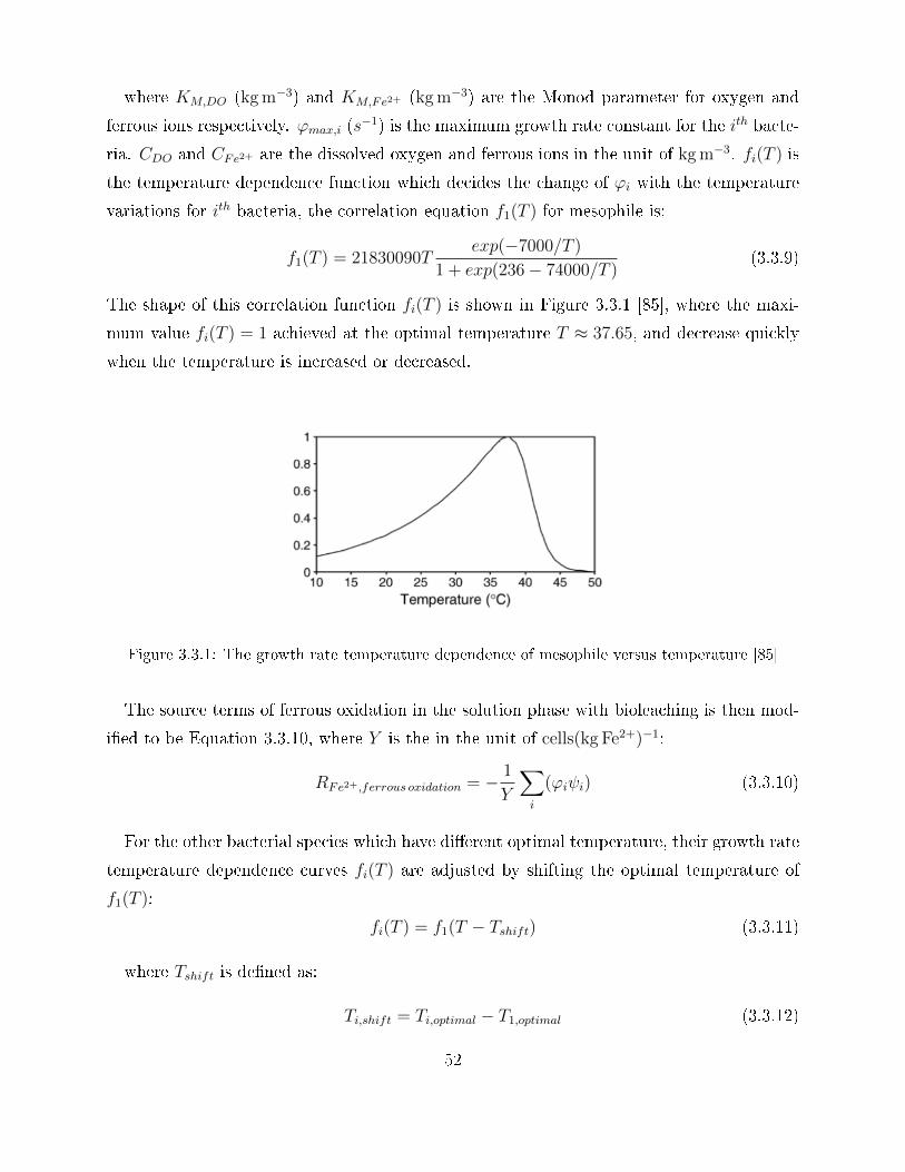
where KM,DO (kg m−3) and KM,Fe2+ (kg m−3) are the Monod parameter for oxygen and

ferrous ions respectively. ϕmax,i (s−1) is the maximum growth rate constant for the ith bacte-

ria. CDO and CFe2+ are the dissolved oxygen and ferrous ions in the unit of kg m−3. fi(T ) is

the temperature dependence function which decides the change of ϕi with the temperature

variations for ith bacteria, the correlation equation f1(T ) for mesophile is:

f1(T ) = 21830090Texp(−7000/T )

1 + exp(236− 74000/T )(3.3.9)

The shape of this correlation function fi(T ) is shown in Figure 3.3.1 [85], where the maxi-

mum value fi(T ) = 1 achieved at the optimal temperature T ≈ 37.65, and decrease quickly

when the temperature is increased or decreased.

Figure 3.3.1: The growth rate temperature dependence of mesophile versus temperature [85]

The source terms of ferrous oxidation in the solution phase with bioleaching is then mod-

ied to be Equation 3.3.10, where Y is the in the unit of cells(kg Fe2+)−1:

RFe2+,ferrous oxidation = − 1

Y

∑i

(ϕiψi) (3.3.10)

For the other bacterial species which have dierent optimal temperature, their growth rate

temperature dependence curves fi(T ) are adjusted by shifting the optimal temperature of

f1(T ):

fi(T ) = f1(T − Tshift) (3.3.11)

where Tshift is dened as:

Ti,shift = Ti,optimal − T1,optimal (3.3.12)

52

The governing equation to calculate the bacteria population attached to the rock is:

∂

∂t(ρsφΨi) = RΨi

(3.3.13)

Then the net growth rate for the population of bacteria attached to the ore is described

as:

RΨi= (ϕi − kdeath,i)ρs(1− φ)Ψi + k1θlψi(1−

Ψi

Ψmax

)− k2ρs(1− φ)Ψi (3.3.14)

3.3.3 Chemical Reaction Rate Kinetics

Empirical reaction rate equations

All the empirical reaction rate equations are listed in Table 3.1. These rate equations

are applied for the dissolution of Chalcopyrite (Equation 3.3.1) and pyrite (Equation 3.3.3),

ferrous oxidation (3.3.5), jarosite precipitations (Equation 3.3.6) and the function for oxygen

solubility. The dissolution of Chalcopyrite and pyrite are nonlinear functions of concentra-

tions on the mineral surface, and k is the pre-exponential factor in the Arrhenius equation

which is tted by experiments. Where the reaction rate constant κ is the function of bulk

uid conditions and calculated by Arrhenius equation. The κ of chalcopyrite and pyrite

dissolutions will be used in the semi-empirical model of Equation 5.3.1 in Chapter 5.

Jarosite precipitation is a switching function which sets the jarosite precipitation rate to

be a constant if the concentration of Fe3+ is higher than a loglinear relationship with pH.

The formation of elemental sulphur in chemical leaching and bioleaching are signicantly

dierent. In chemical leaching by ferric sulphate, almost more than 94% S0 formed by chal-

copyrite dissolution remains as elemental sulphur rather than being oxidised to sulphate [46].

On the other side, with the assistance of sulphur-oxidizing microorganisms in bioleaching,

almost all of the formed S0 is oxidised to sulphate [58]. Due to these extreme phenomena,

we assume the elemental sulphur formed by the chalcopyrite dissolution of Equation 3.3.1 is

dissolving under a rate being linearly dependent on the S0 production rate by chalcopyrite

53

Table 3.1: Empirically derived rates of chemical reaction, and the heat of reactions. All concentra-

tions, denoted by square brackets, have units mol/m3. PO2 is the partial pressure of oxygen, and

DO is the molal concentration of dissolved oxygen.

Kinetic Rate Model

(mol/m3s)

Ea

(kJ/mol)

∆H

(kJ/mol)

Dissolution reactions

Kimball et al (2010) [76]

κCuFeS2

= 4πr2ke−Ea/RT [H+]0.8 [

Fe3+]0.42 48 8.2

Williamson and Rimstidt (1994) [154]

κFeS2

= 4πr2ke−Ea/RT[Fe3+

]0.93 [Fe2+

]−0.4 50 -18.1

Assumed

κS0

= 2µs0κCuFeS2for µs0 ∈ [0, 1]

_ -623.5

Leahy and Schwarz (2009) [87]

κCaCO3

= υCH+,b

_ -35.4

Solution phase and precipitate reactions

Lowson (1982) [96]

κ = 4πr2ke−Ea/RT[Fe2+

]2PO2 [H+]

−0.2574 -102.3

Leahy and Schwarz (2009) [87]

κjarosite = 5.7× 10−5[Fe3+] if log10(0.056[Fe3+

]) > −1.43 pH + 0.87

_ _

Tromans (1998) [144]

DO = PO2 exp[ T8.3144

(0.046T 2 + 203.35T ln(T/298)

− (299.378 + 0.092T )(T − 298)− 20.591× 103)]

_ _

54

dissolution, and µS0 is the linear rate constant that will be calibrated according to the type

of leaching.

Although there are many types of gangue minerals in the chalcopyrite ore, we assume

that the carbonate gypsum, is the typical one to represent the gangue minerals due to the

fact that it has a much faster leaching rate than silicates [87]. The dissolution rate of the

gangue is assumed to be linearly dependent on the bulk acid concentration [87], due to the

important dependence on dissolved oxygen (DO) of ferrous oxidation, the DO is necessary

to be calculated in the simulation, the equilibrium function for the molal concentration of

dissolved oxygen, DO, is chosen and listed in Table 3.1, which is thermodynamics-based.

The heat generation and consumption of each reaction are also listed in Table 3.1, which

are calculated by using the enthalpy of formation of each reactant in the reactions [26,

100, 150]. The Chalcopyrite dissolution of Equation 3.3.1 is slightly endothermic, while the

pyrite dissolution and gang mineral dissolution are moderately exothermic. Both the ferrous

oxidation and dissolution of elemental sulphur are strongly exothermic, which indicate the

net heat generation is positive in the leaching system.

3.4 Basis of The Model

Our mathematical models comprehensively involve following elements:

(1) The chemical reactions include ferric oxidation of chalcopyrite and pyrite disso-

lutions, gangue mineral and elemental sulphur dissolutions, jarosite precipitation and

the biological reaction of ferrous oxidation.

(2) The biological model for the growth and death of microorganisms.

(3) The heat transfer between the solid and liquid phase.

(4) The liquid phase mass transport and heat transfer in a mobile-immobile formula-

tion.

(5) Air transport in the conventional advection-dispersion formulation, with the mass

transfer of of the oxygen between the air and liquid.

55

Being dierent from the current available models from literature, our model innovated

with the following features:

(1) A new semi-empirical, which will be discussed in detail in Chapter 5, is developed

for mineral dissolution, and this model is expected to be more practical to t various

leach kinetics of real ore with the advantage of being computationally ecient.

(2) The transport model is modied to be able to capture the unsteady and inhomo-

geneous distributed mobile and immobile saturations inside the heap which is based on

the ow distribution, also the mass transfer coecient between the mobile and immo-

bile regions and the dispersion coecients of the owing liquid are modied to change

with the ow.

The model is simplied with the following assumptions:

(1) Chalcopyrite is assumed to be the only copper bearing mineral, which is justiable

since the chalcopyrite is the main copper bearing mineral in our ore sample as is listed

in Table 3.2.

(2) The gangue mineral dissolution rate is assumed to be linearly dependent on the

solution acid with a single rate constant, this equation is initially developed for the

dissolution of gangue mineral gypsum [87], although in our ore sample gypsum is not

the main gangue (shown in Table 3.2), this linear algorithm is still used to calculate

the acid consumption by gangue mineral dissolution, but with a modied rate constant

by calibrating with our experiments.

(3) The air is assumed to be under the same temperature of liquid, since the air

density and heat capacity are much smaller than those of the liquid, the air thus will

response to the liquid temperature quickly with the transfer of a small amount of heat.

(4) We assume that heat conduction of rocks throughout the heap is negligible, since

the heat transfer is dominated by advection.

(5) In this thesis, we ignored the inuence of ambient temperature and the heat loss

via evaporation, though those could be included in the future work.

56

(6) We applied the boundary conditions of liquid ow and solution concentrations

homogeneously along the heap top, with no ux boundary conditions along the heap

bottom. The air are assumed to be pumped from the bottom, and the boundary con-

ditions of air ow and oxygen concentration are homogeneously applied along the heap

bottom, no ux boundary conditions along the heap top.

Table 3.2: Main mineral species within ore sample from the experiments used for model developing

and calibration. The data is based on volume percentages [93].

Mineral type vol.%

Copper containing species 1.05

Chalcopyrite 0.58

Covellite 0.15

Cu oxides 0.03

Other Cu minerals 0.29

Pyrite 4.43

Gangue minerals 94.5

Quartz 51.4

Muscovite 39.9

Clays 1.0

Other gangue minerals 2.2

3.5 Conclusion

In this chapter the mathematical formulations of multiphase ow, mass transport and

solid-liquid phase heat transfer of heap leaching are presented, the ow are governed by

Darcy's law, and the transport equations are formulated in a mobile-immobile manner.

The empirical equations proposed by previous literature for the parameters used in the

ow and transport equations are also discussed in this chapter. To model the chemistry in

chalcopyrite leaching, the dominant chemical reactions are proposed and their rate of reaction

57

laws which will be incorporated with the transport model are discussed. The bacterial eect

on ferrous oxidation are considered in our model, and the equations and the parameters

used to determine the bacterial populations and ferrous oxidation rates with bacteria are

discussed. In the following chapter, the ow model, transport model and chemistry model

will be integrated together to simulate the chalcopyrite heap leaching, and the performance

of the leaching system will be analysed by modifying dierent factors and parameters.

58

Chapter 4

Analysis of Base Experiment

To develop the semi-empirical model in Chapter 5, and validate the model code, experimen-

tal data is needed. To accurately estimate the numerical error when comparing simulation

results with experiment data, it is necessary to analyse the experimental error of the exper-

imental results. In this chapter, the experimental error for various solution concentrations

and extractions from the experiment data will be analysed separately.

Three sets of isothermal column leaching data acquired by Lin (2015) [92] are used for

model development and code validation. In the following sections, the kinetics of this sys-

tem will be studied, including the impact of experimental error and uncertainty, in order to

develop suitable models that can form the basis of numerical simulations. The column and

rock conditions were the same for the dierent leaching experiments, and are listed in Table

4.1. Three dierent feed conditions were used and consisted of a base case (K1) from which

ow rate (K2) and ferric to ferrous ratios (K3) were varied (Table 4.2). In addition, 2 re-

peats of K1 were carried out to allow the variability/uncertainty in the results to be obtained.

For each column leaching test, the volumetric change of the mineral grains during leaching

was captured by the micro-CT scanning, which is illustrated in Figure 4.0.1. It is assumed

that the identied mineral grains are the sulphides comprising of copper bearing minerals

and pyrite. In the modelling, chalcopyrite is assumed to be the only copper bearing mineral,

which is justiable because the chalcopyrite minerals constitute a greater proportion of the

ore than the secondary sulphides and oxides (the chemical assay of main mineral species is

listed in Table 3.2 in Chapter 3) and is of the most concern as the dissolution kinetics of

59

Table 4.1: Column and Rock Condition

Parameter value

Column

Height (m) 0.19

Diameter (m) 0.028

Porosity φ 0.4

Absolute permeability (m2

s) 2.3× 10−9

Saturation of Solutes 0.08226

Temperature (C) 60

Rock

Mean diameter (m) 0.01

Cu grade 0.8%

FeS2 grade 4.5%

Table 4.2: The condition of the column experiments

Column Experiment Feed pHFeed Fe3+/Fe2+

(g/L)

Flow rate

(µL/min)

Temperature

(C)

K1 1.2 5/0 80 60

K2 1.2 5/0 40 60

K3 1.2 1/4 80 60

Figure 4.0.1: Micro-CT scan of a single rock, showing the change of extraction of the mineral grains

within a rock. [92]

60

chalcopyrite is the slowest among these leachable copper minerals [11]. The leaching column

was scanned at various time points over the entire leaching period. After image processing,

the total volume of the grains left in the ore particle was obtained. In addition, the amount

of copper and iron in the leachate was measured using ICP (Inductively Coupled Plasma).

This allowed the chalcopyrite and pyrite extraction to be calculated. The extraction was

calculated by averaging over a certain number of rocks with the same sizes within each

column [92]. The calculated extraction of chalcopyrite and pyrite from experiment K1 are

illustrated in Figure A.0.1 in Appendix. The trend in calculated pyrite extraction is more

variable than that of the chalcopyrite as it is based on the dierence between the copper

extraction and that obtained from image analysis, both of which have uncertainties in their

value.

4.1 Experiment Error

The data from the repeated experiments for K1 from Lin(2015) [92], which is presented in

Figure A.0.2 in Appendix, is used to examine the experiment errors and uncertainty. These

repeated tests were carried out simultaneously under the same conditions and using ore from

the same batch.

4.1.1 Copper Extraction and Concentration

The copper extraction varies rapidly with time and in the repeats the measurements are

not all taken at the same time points. This makes the separation of the actual average change

in the value and its variability problematic. One way to do this is to nd an expression that

ts the average behaviour well and then analyse the variations from this behaviour. Key to

this is ensuring that the calculated uncertainty is due to experimental variability and not

problems with the form of the tted curve. The choice of the form is thus important. In this

analysis a set of splines will be used with each of the intervals obeying rst order kinetics.

The overall eect is thus to t a kinetic curve in which the kinetics change with time, but

are assumed constant over short intervals.

61

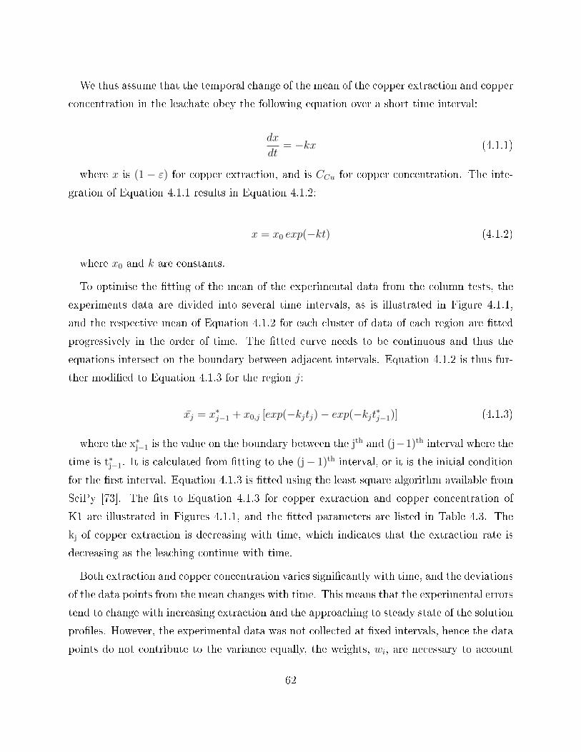
We thus assume that the temporal change of the mean of the copper extraction and copper

concentration in the leachate obey the following equation over a short time interval:

dx

dt= −kx (4.1.1)

where x is (1 − ε) for copper extraction, and is CCu for copper concentration. The inte-

gration of Equation 4.1.1 results in Equation 4.1.2:

x = x0 exp(−kt) (4.1.2)

where x0 and k are constants.

To optimise the tting of the mean of the experimental data from the column tests, the

experiments data are divided into several time intervals, as is illustrated in Figure 4.1.1,

and the respective mean of Equation 4.1.2 for each cluster of data of each region are tted

progressively in the order of time. The tted curve needs to be continuous and thus the

equations intersect on the boundary between adjacent intervals. Equation 4.1.2 is thus fur-

ther modied to Equation 4.1.3 for the region j:

xj = x∗j−1 + x0,j [exp(−kjtj)− exp(−kjt∗j−1)] (4.1.3)

where the x∗j−1 is the value on the boundary between the jth and (j−1)th interval where the

time is t∗j−1. It is calculated from tting to the (j− 1)th interval, or it is the initial condition

for the rst interval. Equation 4.1.3 is tted using the least square algorithm available from

SciPy [73]. The ts to Equation 4.1.3 for copper extraction and copper concentration of

K1 are illustrated in Figures 4.1.1, and the tted parameters are listed in Table 4.3. The

kj of copper extraction is decreasing with time, which indicates that the extraction rate is

decreasing as the leaching continue with time.

Both extraction and copper concentration varies signicantly with time, and the deviations

of the data points from the mean changes with time. This means that the experimental errors

tend to change with increasing extraction and the approaching to steady state of the solution

proles. However, the experimental data was not collected at xed intervals, hence the data

points do not contribute to the variance equally, the weights, wi, are necessary to account

62

(a) Average extraction of copper in the

column

(b) Copper concentration in the leachate

form the bottom of the column

Figure 4.1.1: The mean and experimental errors in the Copper concentration and extraction calcu-

lated from K1, the vertical lines indicate the intervals used to calculate the mean and errors.

Table 4.3: The tted parameters of Equation 4.1.3 for average copper extraction and average copper

concentration

Average Copper Extraction

j 1 2 3 4

kj 0.6 0.142 0.024 0.005

x0,j 0.285 0.352 0.465 0.917

x∗j−1 1.0 0.722 0.604 0.424(1− ε∗j−1)

t∗j−1 0 6 17 53

Average Copper Concentration

j 1 2 3 4

kj 1.315× 10−4 3.121 0.234 0.058

x0,j 3.3475× 104 3.82× 103 10.732 2.618

x∗j−1 20.0 11.201 3.772 1.34(C∗cu,j−1)

t∗j−1 0 2 6 17

for the contribution of each data point, i, to the variance:

s2 =

∑Ni=1wi(xi − xi)2∑N

i=1 wi(4.1.4)

63

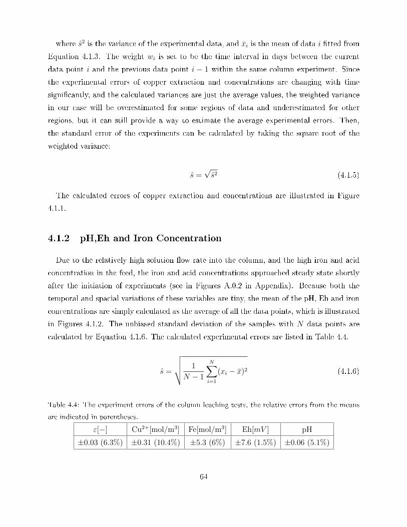
where s2 is the variance of the experimental data, and xi is the mean of data i tted from

Equation 4.1.3. The weight wi is set to be the time interval in days between the current

data point i and the previous data point i − 1 within the same column experiment. Since

the experimental errors of copper extraction and concentrations are changing with time

signicantly, and the calculated variances are just the average values, the weighted variance

in our case will be overestimated for some regions of data and underestimated for other

regions, but it can still provide a way to estimate the average experimental errors. Then,

the standard error of the experiments can be calculated by taking the square root of the

weighted variance:

s =√s2 (4.1.5)

The calculated errors of copper extraction and concentrations are illustrated in Figure

4.1.1.

4.1.2 pH,Eh and Iron Concentration

Due to the relatively high solution ow rate into the column, and the high iron and acid

concentration in the feed, the iron and acid concentrations approached steady state shortly

after the initiation of experiments (see in Figures A.0.2 in Appendix). Because both the

temporal and spacial variations of these variables are tiny, the mean of the pH, Eh and iron

concentrations are simply calculated as the average of all the data points, which is illustrated

in Figures 4.1.2. The unbiased standard deviation of the samples with N data points are

calculated by Equation 4.1.6. The calculated experimental errors are listed in Table 4.4.

s =

√√√√ 1

N − 1

N∑i=1

(xi − x)2 (4.1.6)

Table 4.4: The experiment errors of the column leaching tests, the relative errors from the means

are indicated in parentheses.

ε[−] Cu2+[mol/m3] Fe[mol/m3] Eh[mV ] pH

±0.03 (6.3%) ±0.31 (10.4%) ±5.3 (6%) ±7.6 (1.5%) ±0.06 (5.1%)

64

(a) The redox potential of the leachate

form the bottom of the column

(b) The concentration of iron the

leachate form the bottom of the column

(c) pH of the leachate form the bottom of the col-

umn

Figure 4.1.2: The mean and experiment error of Eh, Fe concentration and Ph calculated from K1

4.2 Dissolution Kinetic Analysis

In the following kinetic analysis of the column leaching, both the horizontal and vertical

variations of solutions and extractions are neglected so that the analysis is based on a zero

dimensional test. The assumption of simplifying the original 3-D test to 0-D test is reason-

able, because the diameter of the column is small and thus the horizontal variations can be

ignored. Given the high solution feeding rate and slow kinetics, the vertical length of the

column is also small and the feeding solution concentration of Fe3+ is much higher than the

consumption rate, hence the leachate condition reached a steady state which is similar to

65

the feeding solution condition quickly, and the transient period is short enough that it can

be neglected compared with the long leaching period, thus the vertical variations can be

reasonably neglected.

4.2.1 Analysis with SCM

In the 0-D model, we can treat the whole column as a a set of particles surrounded by

solution with the out ow concentration. We can therefore directly t the data using the

shrinking core and similar models introduced in the previous chapters. The diusion control

through the ash layer, Equation 2.3.23, and the chemical reaction control, Equation 2.3.26,

versions of this model, which are introduced in Chapter 2, will be studied.

From Figures 4.2.1(a) to 4.2.1(c), it can be seen that all of the column tests (K1, K2, K3)

have a better t using diusion control rather than the chemical reaction control equations.

This implies that in those column tests the surface reaction rates are high compared to the

diusion rate through the ore particles. Previous researchers [62,88] have indicated, though,

that factors such as wide grain size distributions can inuence this interpretation.

(a) The calibration of K1 with SCM.

Blue solid line: diusion control. Red

dotted line: reaction control.

(b) The calibration of K2 with SCM.



66

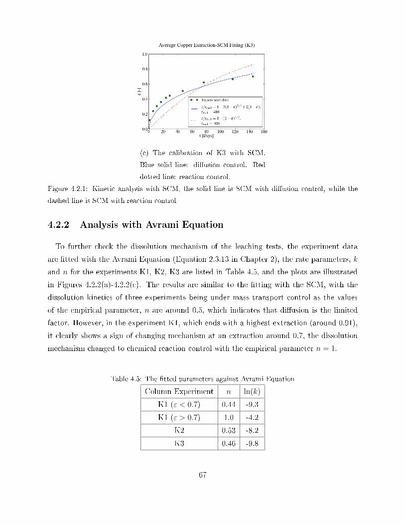
(c) The calibration of K3 with SCM.



Figure 4.2.1: Kinetic analysis with SCM, the solid line is SCM with diusion control, while the

dashed line is SCM with reaction control

4.2.2 Analysis with Avrami Equation

To further check the dissolution mechanism of the leaching tests, the experiment data

are tted with the Avrami Equation (Equation 2.3.13 in Chapter 2), the rate parameters, k

and n for the experiments K1, K2, K3 are listed in Table 4.5, and the plots are illustrated

in Figures 4.2.2(a)-4.2.2(c). The results are similar to the tting with the SCM, with the

dissolution kinetics of three experiments being under mass transport control as the values

of the empirical parameter, n are around 0.5, which indicates that diusion is the limited

factor. However, in the experiment K1, which ends with a highest extraction (around 0.91),

it clearly shows a sign of changing mechanism at an extraction around 0.7, the dissolution

mechanism changed to chemical reaction control with the empirical parameter n = 1.

Table 4.5: The tted parameters against Avrami Equation

Column Experiment n ln(k)

K1 (ε < 0.7) 0.44 -9.3

K1 (ε > 0.7) 1.0 -4.2

K2 0.53 -8.2

K3 0.46 -9.8

67

(a) The calibration of K1 with Avrami

Equation

(b) The calibration of K2 with Avrami

Equation

(c) The calibration of K3 with Avrami

Equation

Figure 4.2.2: Kinetic analysis of the experiment results with Avrami Equation.

This transition might indicate that the reaction rates decreased signicantly after the ex-

traction reached 0.7, and the later dissolution rates is limited by a slow down in the reaction

rate. This might be caused by the depletion of the other faster reacting copper bearing

minerals, such as secondary sulphide minerals and oxides copper minerals. As it is listed

in Table 3.2 in Chapter 3, the secondary sulphide minerals, copper oxides and other copper

minerals contributed to around 45% of the total copper bearing mineral in volume. Initially,

the extraction of copper is mainly contributed by the dissolution of these fast reacted copper

bearing minerals, as the dissolution of slowest primary ore (mainly chalcopyrite) is much

slower, thus the extraction rate is fast and the dissolution is under diusion control. With

68

the depletion of these fast reacted copper bearing minerals, the extraction rate of copper de-

clines and the dissolution of the slow reacted primary ore become the major source of copper

extraction, and thus the mechanics of dissolution changes to the reaction control. Due to the

lack of the experimental data from the other two experiments, where highest extractions are

0.73 for K2 and 0.7 for K3, it could not be determined whether this transition is universal

or not. Also, because the Avrami Equation is a semi-empirical model, the law might not

t our experiments well, so it is hard to conrm whether this change is due to a change in

mechanism or the appropriateness of the model.

The results of the analysis with the Avrami Equation indicate that xing of the kinetic

model with either diusion control or reaction control in the simulation might not be ap-

propriate. Although it is possible to change the dissolution mechanism in the numerical

simulation when the extraction reached to a certain point, as done by, for instance, Bennett

et al. [15] in their copper leaching simulation, it is hard to conrm that critical point in

our case. Therefore, a more exible kinetic model is desirable in our simulation, which can

t the dissolution mechanism reasonably whether it is under diusion control, reaction con-

trol or even mixed control, but without the need to manually select the appropriate kinetic

model. To meet this requirement, an innovative semi-empirical model is developed and will

be introduced in the following Chapters.

4.3 Conclusion

In this chapter, the experimental conditions of the base experiments (K1, K2 and K3) are

introduced, the experimental data of the experiment K1 will be used to develop the semi-

empirical model in Chapter 5. The experimental errors of this base experiment are analysed,

which are based on the data collected from three repeated experiments, separate errors are

calculated for copper extraction, copper concentration, Eh, pH and iron concentration. These

experimental errors indicate the accuracy of the experiment operations and measurements,

and measure how these experimental data is to the true value. To validate the developed

computational model, these errors along with the experiment K2 and K3 will be used in

Chapter 6. The dissolution kinetics of the three experiments are analysed with the SCM

and Avrami equation, and the results indicate that changing of the dissolution kinetic might

69

occur during leaching, the traditional SCM which xes the kinetic with either reaction control

or diusion control might not be proper. Therefore, a new semi-empirical model will be

developed in Chapter 5 to provide a more exible approach for numerical modelling of

leaching system.

70

Chapter 5

A New Semi-empirical Model for

Leaching

As discussed in the previous chapter on the kinetic analysis of our experiment (Section

4.2), the Avrami parameters indicate that our experiment might undergo a transition in the

dominant dissolution kinetic mechanism during leaching, thus the conventional SCM with

either diusion alone or reaction alone may not be appropriate for the modelling of this

system. Moreover, real ores contain a range of particle sizes each with a range of grain sizes

within them. Those properties are hard to capture within shrinking core type models. In

this chapter, a framework for directly using laboratory scale experimental data to predict

the heap scale performance in a computationally ecient manner will be presented. This

framework provides an alternative to the shrinking core model that is more exible in ability

to t with various dissolution kinetics proles.

5.1 Theoretical Basis

The key assumption of this modelling approach is that the eect of the bulk uid conditions

(concentrations, temperatures, pH etc.) and the current state of the particles (characterised

by the current extent of extraction, ε) on the leaching rate are mathematically separable,

an assumption shared with most shrinking core type models. This means that the leaching

rate of a particular mineral species at a particular location in the heap can be expressed as

71

follows:dε

dt= κ(C1b, C2b, T, etc)f(ε) (5.1.1)

where κ is a function of bulk uid conditions, subscript b refers to the bulk concentrations.

These concentrations, as well as the extents of reaction of each of the mineral types, will be a

function of time and position within the heap. The chemical dependency could be obtained

experimentally, but literature values will be used in this work. So we calculate κ using the

equations listed in Table 3.1 in Chapter. 3.

The validity of this separability assumption is discussed below. To analyse separability,

we need to consider what is happening at three dierent scales:

Grain scale

If a single grain within the rock is considered, then we can write out the kinetics of

dissolution of that grain, i, in terms of its surface reaction kinetics:

ρmdVidt

= −f(ri)ke−Ea/RTCm11 Cm2

2 (5.1.2)

Where the concentrations are those within the rock at the surface of the grain ρm is the

molar density of the grain, Ea is the activation energy and f(ri) is the surface area of the

grain.

In a more generic form this can thus be written as:dVidt

= −f(ri)κ(C1, C2, T, etc) (5.1.3)

At the scale of a single grain the behaviour is thus mathematically separable. If we now

consider all the mineral grains within a small volume of the rock, that are all experiencing the

same chemical conditions, but which have dierent sizes and surface areas, or equivalently,

consider all these grains within an entire rock that experience the same chemical conditions.

The overall leaching rate of all these grains can thus be expressed as follows:

dV

dt= −κ(C1, C2, T, etc)

N∑i=0

f(ri) (5.1.4)

72

The behaviour is thus still separable for a collection of dierent sized grains all experiencing

the same chemical conditions, where V is the sum of the volumes of the mineral grains.

Rock scale

Within a single rock the chemical conditions can be a function of position due to the

competing eects of surface reaction and diusion. If the position within the particle is

characterised using the vector, X , then the overall behaviour of the individual rock will be

separable if the `driving force', κf , can itself be expressed in a separable form:

κf (X) = κ(C1b, C2b, Tb, etc)g(X) (5.1.5)

Where:

κf (X) = κ(C1, C2, T, etc) (5.1.6)

Importantly, g(X) is not a function of κ. This is actually an assumption and will not

be universally true. It is true, though, if the concentrations are at pseudo-steady state (a

reasonable assumption given the slow kinetics of most heap leaching systems) and the be-

haviour is either reaction limited or the surface reactions are linear or the system is diusion

limited in terms of one of the reagents (though this will change the form of κ). In non-

linear systems which are neither reaction nor diusion limited this assumption will not be

completely true, but the eect of this assumption is still likely to be a smaller eect than

that of, for instance, the grain size and particle size distributions and is thus worth making.

Given enough experimental or small scale simulation data this assumption can be relaxed

by making use of a family of curves rather than a single curve.

Bulk scale

If the behaviour of a single rock particle is separable in terms of the eect of bulk chemistry

and its current state of leaching on its leaching rate, then the behaviour of a collection of

these particles all experiencing the same chemical conditions will also be separable for very

similar reasons to why the overall behaviour of a group of dierent sized mineral grains

experiencing the same chemical conditions are separable.

73

5.2 Validation of The Separability Assumption

To demonstrate that the assumption that the behaviour is separable is reasonable, we will

model the behaviour using shrinking core model with non-linear surface kinetics. Unlike the

standard shrinking core model, which assume linear kinetics, this system is not inherently

separable. This analysis is being carried out as the surface leach kinetics for chalcopyrite is

known to be nonlinear. In this analysis, we consider the following generic leaching reaction

in which reagent A reacts with solid reactant B:

A+ bB → products (5.2.1)

We will validate the separability assumption using a non-dimensionlised version of the

equations to limit the parameter space that needs to be studied [48]. According to Wen

(1968), Dixon and Hendrix (1993) [38, 153], the internal reagent concentrations inside an

ore CA, the solid reactant concentration inside an ore CB, radius r and time t can be

nondenominationalised as:

CA =CACA0

, CB =CBCB0

, ξ =r

r0

, τ =t

tD(5.2.2)

Where CA0 and CB0 are the reference concentrations, r0 is the radius of the ore particle, and

tD is a characteristic diusion time:

tD =φr2

0

De

(5.2.3)

where φ is the porosity of the particle.

We further dene a dimensionless reagent concentration external to the ore particle CAb,

stoichiometric ratio β, shrinking core reaction modulus κc which is the Damkohler II number:

CAb =CAbCA0

, β =φbCA0

CB0

, κc =ksr0C

o−1A0 C

mB0

bDe

(5.2.4)

74

where m and o are orders of reaction, ks is a surface reaction rate constant, and the

reaction modulus κc represents the ratio of reaction rate to diusion rate. The governing

equation for the shrinking core model in dimensionless form may now be written:

∂C

∂τ=

1

ξ2

∂

∂ξ

(ξ2∂C

∂ξ

)(5.2.5)

The governing equation describes the diusion transport through the leached outer portion

of the particle. The boundary and initial conditions for Equation 5.2.5 are:

C = CAb at ξ = 1, (5.2.6a)

∂C

∂ξ= κcC

o at ξ = ξc, (5.2.6b)

∂C

∂ξ= − 1

β

dξ

dτat ξ = ξc, (5.2.6c)

ξc = 1 at τ = 0 (5.2.6d)

where ξc is the dimensionless core radius.

By making a pseudo-steady state assumption, which is generally valid when β is small

[91, 153], we can simplify the Equation 5.2.5 by neglecting the term ∂C/∂τ . The equation

then reduces to an implicit ordinary dierential equation once the boundary and initial

conditions have been applied:

1

β

dξcdτ

+ κc

[CAb + ξc (1− ξc)

1

β

dξcdτ

]o= 0 (5.2.7)

Since Equation 5.2.7 is implicit, it is computationally expensive when coupled with the

heap leaching simulation, especially for a large scale model with numerous elements and

long simulation times. Thus it is desirable to simplify the implicit SCM Equation 5.2.7

into an explicit equation, though it is recognised that this will introduce approximation

inaccuracies. As mentioned in Section 2.3.4, the SCM can be reduced to an explicit model

and solved analytically when it is reaction controlled (κc ≈ 0) with linear reaction kinetics,

or diusion controlled (κc 1), or mixed control with linear reaction kinetics (o = 1).

However, in reality, especially in chalcopyrite leaching, the reaction rate and diusion are

both comparably important, and the reaction kinetics are nonliear [76,98]. While using the

75

assumptions that result in true separability is likely to be inaccurate, an improved explicit

equation which can be used for non-linear reaction kinetics with mixed control is desirable.

We propose a new explicit model which is semi-empirical and is expected to be able to t

the leaching models with various dissolution mechanisms. The key assumption of this model

is that the nonlinear dependence on the bulk uid conditions CAb is separable from the

dependence on the current state of the core ξc. To demonstrate this separability assumption,

we rstly propose that Equation 5.2.7 may be approximated by a modication to the SCM

with linear kinetics, so with o = 1, Equation 5.2.7 reduces to:

1

β

dξcdτ

=CAb

1/κc + ξc(1− ξc)(5.2.8)

Then we suppose that the eects of nonlinearity is now replaced with some nonlinear

scaling, Cn′ext:

1

β

dξcdτ

=Cn′ext

1/κc + ξc(1− ξc)(5.2.9)

Finally, Equation 5.2.9 can be integrated and solved analytically:

τ =1

βCn′Ab

[1− ξcκc

+1− 3ξ2

c + 3ξ3c

6

]=

1

βCn′Ab

[1− (1− ε)1/3

κc+

1− 3(1− ε)2/3 + 3(1− ε)6

] (5.2.10)

Where ε is the current state of extraction:

ε = 1− ξ3c (5.2.11)

From Equation 5.2.10, it can be seen that when κc 1, the equation is reduced to the

SCM with diusion control of Equation 2.3.23 in Section 2.3.4 by neglecting the small term

of 1−(1−ε)1/3κc

. When κc ≈ 0, the term of 1−3(1−ε)2/3+3(1−ε)6

then become much smaller than the

rst term in Equation 5.2.10, and thus it can be approximated to the SCM with reaction

control of Equation 2.3.26 in Section 2.3.4.

Obviously, Equation 5.2.10 is a separable form of 5.1.1. To demonstrate this form is rea-

sonable, it is necessary to analyse the errors arising from the non-linearity of the dissolution.

76

Therefore, n′ in Equation 5.2.10 is computed numerically for a wide range of o, CAb, κc to

achieve the best least squares match to Equation 5.2.7. The Assimulo dierential algebraic

solver [6] is used to integrate Equation 5.2.7 over βτ , and then n′ in 5.2.9 is optimised using

the Brent algorithm in SciPy [73] to obtain the minimum least squares error in ε compared to

the one calculated from Equation 5.2.7. Errors are evaluated over the full range of extraction

(0 ≤ ε ≤ 1).

Figure 5.2.1: Optimisation of n′ for the new explicit model over a wide range of κc, with associated

extraction errors

One example is illustrated in Figure 5.2.1, where o = 0.42 and CAb = 0.2. It shows how

n′ and the associated extraction errors | ε′ − ε | change over the range of κc. The maximumerror occurs around κc = 10, which implies a dissolution mechanism that is non-linear with

mixed control. The maximum error is around 5% and the time-averaged error is around

Figure 5.2.2: Extraction curve for the worst case with κc = 10

77

2% with an R2 coecient of determination of 99%. It also shows that n′ is bounded within

0.42 to 1. n′ approaches 0.42 under reaction control when kc ≈ 0 and approaches 1 under

diusion-control when kc 1. The errors are becoming small when the dissolution is under

either reaction-controlled or diusion-controlled and thus when the SCM is separable as

expected. An average error of 2% and maximum error of 5% under the worst conditions

means that this assumption of separability is reasonable, especially given the other likely

sources of error in the system and the computational cost saving that an explicit equation

allows relative to an implicit one. The extraction curves for the worst case when κc = 10

is illustrated in Figure 5.2.2. Figures 5.2.1 and 5.2.2 show that the approximation of the

new explicit model to the implicit non-linear SCM is satisfactory with small errors even for

the worst case, while the explicit model is much computationally ecient than solving the

model implicitly.

Figure 5.2.3: The peak errors over a range of non-dimensional external concentrations and selected

intrinsic reaction orders

From Figure 5.2.3 for the peak errors for various o and CAb, it can be seen that the

inaccuracy will increase as o and CAb diverge from unity. This means the inaccuracies will

increase with the increasing non-linear eects when the reaction order diers from unity,

and with the solution concentration diering from the the reference calibration value. If

separability is to be assumed it is thus important to use calibration experiments under

chemical conditions close to those that are likely to be experienced by the heap.

78

5.3 Calibrating The Model

As has been mentioned before, in the small scale leaching tests, the volumetric change

of the mineral grains during leaching was captured by the micro-CT scanning. We can

therefore get the extraction as a function of time from the small scale leaching tests. We

choose the data from base experiment of K1 to directly calibrate our model and will use

the other experiments for validation. Under the separability assumption, we can rewrite

Equation 5.1.1 as follows:

dε

dt

1

κ= f(ε) (5.3.1)

Figure 5.3.1: The semi-empirical curve interpolated by cubic spline, dεdt1κ Versus ε, of copper extrac-

tion.

We assume in this work that the form of κ is the same as that for the surface reactions

listed in Table 3.1 in Chapter 3, though this could be obtained experimentally as well. As

this is a small column, it is reasonable to assume that the concentrations at the outlet

are representative of those within the column. Thus by applying the outlet concentrations,

which are changing with time, to the equations of surface reactions (represented by κ), κ is

known as a function of time for the experiment. The dε/dt in the left hand side of Equation

5.3.1 can be obtained by numerically dierentiating the curve of the extraction rate from

experiment (the curves of mineral extraction rate are listed in Figure A.0.1 in Appendix). If

79

the curve of extraction rate had been noisy either smoothing or curve tting would need to

be used. The left hand side of Equation 5.3.1 can thus be calculated and plotted in Figure

5.3.1. The data points in Figure 5.3.1 are interpolated by using a cubic spline interpolation.

This graph thus represents Equation 5.3.1 and is used within the simulation as a lookup

table with interpolation between the points.

5.4 Conclusion

A new semi-empirical model for mineral dissolution is presented in this chapter. Being an

alternative to the traditional SCM approaches, it can t various dissolution kinetics proles

with a single model and thus is more exible than SCM approaches which use dierent

mathematical models for dierent dissolution kinetics. The validity of the key separability

assumption of this model has been veried, and it is suggested that the maximum error

caused by this assumption is less than 5% when the leaching system is under mixed control

and highly non-linear, thus, this model is supposed to be able to predict the leaching system

with any dissolution kinetics satisfactorily. Finally, the experimental data from K1 is used

to calibrate our model, and a tted semi-empirical curve will be used as a lookup table to

predict the dissolution rates in the following chapters. The validation of the numerical model

using this semi-empirical model will be presented in the next chapter.

80

Chapter 6

Numerical Scheme and Model Validation

Before Implementation of numerical modelling, the numerical discretizations of the ow

and transport equations in our model are introduced in this chapter. Also, it is necessary

to verify or validate the code by analytical solutions or experimental data before doing heap

leaching simulations, so that the numerical simulator can be conrmed to be coded in a

proper way and without any bugs that will cause signicant inaccuracy.

6.1 Numerical Framework

Fluidity, an open source code which is an unstructured mesh based nite element/control

volume simulator, is used to model the mass transport and heat transfer within the heap

leaching system [5]. The mass transport and heat transfer model is based on the previous

multiphase ow model developed by Mostaghimi et al. [107] for ow in porous media, in

which the numerical scheme of control volume nite element method (CVFEM) along with

the implicit pressure, explicit saturation algorithm (IMPES) is employed [107].

This chapter starts by describing the discretization of the ow equations, followed by the

scheme used for solving the mass and heat transfer equations. The nal section of this chap-

ter explores a number of verication and validation test cases.

81

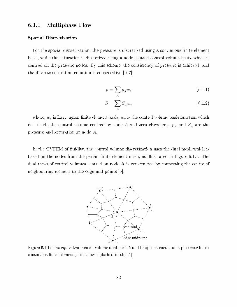
6.1.1 Multiphase Flow

Spatial Discretization

For the spacial discretization, the pressure is discretized using a continuous nite element

basis, while the saturation is discretized using a node centred control volume basis, which is

centred on the pressure nodes. By this scheme, the consistency of pressure is achieved, and

the discrete saturation equation is conservative [107]:

p =∑A

pAwe (6.1.1)

S =∑A

SAwv (6.1.2)

where, we is Lagrangian nite element basis, wv is the control volume basis function which

is 1 inside the control volume centred by node A and zero elsewhere. pAand S

Aare the

pressure and saturation at node A.

In the CVFEM of uidity, the control volume discretization uses the dual mesh which is

based on the nodes from the parent nite element mesh, as illustrated in Figure 6.1.1. The

dual mesh of control volumes centred on node A is constructed by connecting the centre of

neighbouring element to the edge mid points [5].

Figure 6.1.1: The equivalent control volume dual mesh (solid line) constructed on a piecewise linear

continuous nite element parent mesh (dashed mesh) [5]

82

The Petrov-Galerkin weighted residual method is used to form the linear system for pres-

sure [107]. To ensure the continuity within each control volume, the global continuity Equa-

tion 3.1.6 in Chapter 3 is weighted by the control volume basis function and integrated over

the whole domain. Since the control volume weighted function is zero everywhere outside

the each local control volume (CV), the integration of the global continuity equation can

be reduced to the integration of the continuity for each local CV. Then by adopting the

divergence theorem the linear system can be further reduced to be the integrations over the

surfaces of the control volumes, which is [107]:∫∂cv

n · [∑i

Ki

µi(∇pi − ρig)] = 0 (6.1.3)

where ∂cv is the surfaces for the control volume, and n is the outward pointing normal. The

linear system for saturation can be obtained by integrating and weighting Equation 3.1.3 in

a similar way, ∫cv

φ(Si)

∂t−∫∂cv

n · [Ki

µi(∇pi − ρig)] = 0 (6.1.4)

where cv is the domain of the control volume.

Time Discretization

The implicit pressure explicit saturation algorithm (IMPES) is used to solve the multiphase

ow in porous media. To solve for the system at time n + 1, the pressure is calculated

implicitly based on the saturation at time n [107]:∫∂cv

n · [∑i

Kni

µi(∇pn+1

i − ρig)] = 0 (6.1.5)

The solved pressure at time n+1 and the saturation at time n are used to solve for saturation

at time n+ 1 explicitly using Equation 3.1.3 in Chapter 3:∫cv

φ(Sn+1i − Sni )

∆t=

∫∂cv

n · [Kni

µi(∇pn+1

i − ρig)] (6.1.6)

6.1.2 Mass Transport and Heat Transfer

In heap leaching, various chemical species in the solution are transported throughout the

packed bed, where several chemical reactions take place, consuming and generating chemical

83

species and heat. To achieve the conservation of mass and heat transport, the nite vol-

ume method is applied, so that the mass and heat are discontinuous through each element.

Within each element of the nite volume, the concentrations and temperature are constant,

and the particles packed within each element are assumed to under the same extraction rate.

Spatial Discretization

The scalar transport of both concentration and temperature are discretized by lowest or-

der discontinuous Galerkin method which is centred on the nite element mesh, so that the

elds are conservative, which is illustrated in Figure 6.1.2. The shape function wdg has value

1 at node A and across each control volume element, but zero elsewhere:

c =∑A

cAwdg (6.1.7)

Figure 6.1.2: The piecewise constant, element centred shape function of lowest order discontinuous

Galerkin method [5]

.

To generate the weak form of the transport Equations 3.2.1 in Chapter 3, the equations

are weighted by the nite volume basis function and integrated over the whole domain, Ω:∫Ω

wdg[∂θc

∂t+∇ · (uθc)−∇ · (¯k · θc)] =

j∑∫Ω

Rj \Qj −∫

Ω

δc (6.1.8)

By integrating by parts of both the dispersion and advection terms, and by adopting the

84

divergence theorem, the linear system for the transport of scalar eld c is formed:∫Ω

[wdg∂θc

∂t−∇wdg ·uθc+∇wdg · ¯k·θc]+

∫∂Ω

wdg[n·uθc−n·(¯k·θ)·∇c] =

j∑∫Ω

Rj \Qj−∫

Ω

δc

(6.1.9)

Since the nite volume weighted function is zero everywhere outside each local nite

volume (fv), the integration of the transport equations can be reduced to the integration of

the continuity for each local fv. Also, because the shape function wdg has value 1 within

each fv, the function is now further reduced to [5, 121]:∫fv

∂θc

∂t+

∫∂fv

[n · uθc− n · (¯k · θ) · ∇c] =

j∑∫fv

Rj \Qj −∫fv

δc (6.1.10)

where c is either concentrations Ci or temperature terms CpρT , where the product, CpρT ,

represents the heat enthalpy per volume, which is a conserved quantity. ¯k is either the

dispersion coecients or thermal diusivity, Rj \Qj is the source terms from the jth reaction,

either amount of reagent i produced per volume or the heat released by the reaction per

volume. δc is the coupled mass or heat transfer terms between mobile-immobile liquid or

solid-liquid phase, as is described in Equation 3.2.5 and Equation 3.2.17 in Chapter 3.

Time Discretization

The coupled system of mobile and immobile concentrations, solid and liquid temperatures

are solved implicitly while the chemical source terms are calculated explicitly, that is:∫fv

(θn+1cn+1m )− (θncnm)

∆t+ Mn+1cn+1

m +

∫fv

δcn+1m =

j∑∫fv

Rnj,m \Qn

j,m (6.1.11)

∫fv

(θn+1cn+1im )− (θncnim)

∆t−∫fv

δcn+1im =

j∑∫fv

Rnj,im \Qn

j,im (6.1.12)

where M is the matrix:

Mn+1 =

∫∂fv

[n · un+1θncn+1m − n · (¯kθn+1) · ∇·] (6.1.13)

The transfer term δc is:

δcn+1m/im = αm,im

(cn+1m − cn+1

im

)(6.1.14)

85

for mass transport equations, or:

δcn+1m/im = (+/−)ωn+1

m/imhtan+1t (cn+1

s − cn+1l ) + αm,im(cn+1

m − cn+1im ) (6.1.15)

for heat transfer equations, where the subscripts m,im represent the mobile and immobile

elds, and s, l represent the solid and liquid phase.

The reaction of chalcopyrite, pyrite and ferrous oxidation, gangue mineral and elemental

sulphur dissolutions are regarded as reacting simultaneously with the same values of concen-

trations. In other words, the rates of these reactions are based on the same concentration at

time step n without any priority, and the calculated reactions are included in the source term

Rj \Qj. The equilibrium of the oxygen dissolution and jarosite precipitations are calculated

when all other reactions have completed and the concentrations have been updated. This is

because we assume that the equilibrium reaction is fast enough to respond to other slower

reactions, and then change the concentrations to achieve equilibrium. Thus, we assume the

dissolved oxygen achieves equilibrium and the solubility of ferrics are based on the pH at

the end of each time step, when all the concentrations have been calculated by the mass

transport equations.

For the reaction of chalcopyrite and pyrite, the rate of extraction, dε/dt , is calculated

explicitly by passing simulated values for the concentrations and extracted fractions into the

semi-empirical model based on Equation 5.3.1. Then the source term in Equation 3.2.1 due

to the dissolution of the chalcopyrite and pyrite will be:

Rnj = [Np npκ

nf(εn)]m=FeS2\CuFeS2

(6.1.16)

Where Np is the total molar amount of the mineral per rock, and np is the number of

rocks per unit volume of the heap. The source terms from other reactions are also calcu-

lated explicitly by using the kinetic rate equations listed in Table 3.1 in Chapter 3. The

coupling between the species are related by the stoichiometric factors from the chemistry

equations, and the corresponding sources are added into the transport equations accordingly.

86

Source Term Linearization

The concentrations in our transport equations are always non-negative values, however,

since the leaching chemistries are strongly coupled, these non-negative quantities may have

both positive and negative source terms, and the resultant net source term can lead the

elds to an erroneous negative value, especially with large time steps. To ensure physically

realistic results as well as to allow a large time step in our model, we modied the chemical

source terms in the transport equations by using source linearization, which is proposed by

Patankar (1980) [119]. The linearization method is as follows:

Assuming that the total source term of species, i, are made up of the positive source terms

R+i and negative source terms R−i :∑

Ri =∑

R+i +

∑R−i where R+

i > 0, R−i < 0 (6.1.17)

The net source term is linearized by the species concentration Ci:∑Ri =

∑R+i +

∑R−iCni

Cn+1i (6.1.18)

where Cni is the current value of concentration, while Cn+1

i is the concentration at the new

time to be solved. By applying the Equation 6.1.18 in the model, the negative source term

can be moved to the left hand side of the matrix and are solved implicitly, which can avoid

negative concentrations.

6.2 Verication and Validation of Code

To ensure the numerical model is properly coded, verication and validation of the model

is necessary. Both the mobile-immobile model and semi-empirical model are validated with

experimental results, while the two phase heat transfer model is veried with the method of

manufactured solutions due to the lack of experiment data.

6.2.1 Validation of The Mobile-imobile Model

The numerical simulation of the mobile-immobile model was solved in a domain representa-

tive of the experimental work presented by Ilankoon et al. [70]. In their column experiments,

87

the 18 mm non-porous glass beads were used as the packing particle and packed in a Perspex

column. The experimental setup is illustrated in Figure 6.2.1. The liquid was rstly intro-

duced to the packed bed in the experiment, and once the liquid ow rate inside the column

achieved steady state, a pulse of calcium chloride (CaCl2), which was used as a tracer, was

injected into the bed from the top of the column. The salt concentration exiting the column

was obtained by measuring the euent conductivity at the outlet of the column. According

to the experiment results, the residence time distribution (RTD) curve captured a long tail,

which disagrees with the convectional advection-dispersion model [70], thus indicating the

requirement for the mobile immobile model. In these simulations the bed dimensions and

porosity, as well as the liquid addition rate and physical properties of the uid were based

on the experimental values, where as absolute permeability and relative amounts of liquid

in the mobile and immobile regions were related as tting parameters.

Figure 6.2.1: The experimental setup of the tracer test for the immobile-mobile model [70]

The residence time distribution (RTD) function, also called exit-age distribution function

E(t), is the function that describes the amount of time that a uid element has resided in the

column, and it denes the age distribution of the euent stream, and has the unit of time−1.

The quantity E(t)dt denes the fraction of a uid element exiting the reaction between t

and t+ dt [50]:

E(t) =C(t)∫∞

0C(t)dt

(6.2.1)

88

The cumulative RTD function (F(t)) is calculated by summing the exit-age distribution

function (E(t)) over all times [50], which are:

F (t) =

∫ t

0

E(t)dt (6.2.2)

This quantity represents the fraction of a uid element that has resided in the column for

less than time t, and F (t) should be equal to 1 if t =∞.

Table 6.1: Column and Rock Condition

Parameter value

Column

Height, z (m) 0.3

Diameter (m) 0.243

Porosity, φ 0.4

Absolute permeability, ka (m2

s) 1.77× 10−9

Liquid

Total liquid hold-up, θw 0.18

Dynamic liquid hold-up, θd 0.11

Darcy velocity, uw (m/s) 1.5× 10−5

Dynamic viscosity, µw (kg/(m · s)) 1.0× 10−3

Air

Pressure, pa (Pa) 1.0× 105

Dynamic viscosity, µa (kg/(m · s)) 1.725× 10−5

The experiment conditions and parameters are listed in the Table 6.1, where the solution

ow is at steady state. The simulation is implemented in 1D since the lateral variations of

the ow could be ignored [70]. As the purpose of these simulations is to test mass transport,

the uid ow boundary conditions and initial values are set to be their steady state values

so that they do not vary with time:

va|z=bottom = 0 (6.2.3)

va|z=top = 0 (6.2.4)

Sw(0, z) =θiφ

= 0.0295 (6.2.5)

89

vw|z=top = −1.5× 10−5 (6.2.6)

where va is the Darcy velocity of air and vw is the Darcy velocity of the liquid. The pressure

of the water is assumed to be purely gravity driven. To solve the mass transport problem,

the initial condition of tracers is set to be:

Cj,im(0, z) = 0 (6.2.7)

Cj,m(0, z) = 0 (6.2.8)

While the boundary condition is set to be the Dirac delta function, in order to introduce a

tracer pulse from the top of the bed at the beginning of the simulation:

Cj,m(t, 0) = δ(t) (6.2.9)

Figure 6.2.2: Comparison of the CFD simulation results for the mobile-immobile model with the

experiment results

The simulation results are compared with experiment result from Ilankoon et al. [70],

which is illustrated in Figure 6.2.2. Six dierent simulation mesh sizes are used in the sim-

ulations, which are 0.16, 0.08, 0.04 and 0.02, 0.01, 0.005 (m). It can be observed that the

mobile-immobile model approximates the experiment result well, and the simulations con-

verge to the experiment when increasing the resolution of the mesh. According to Figure

6.2.3, the calculated l2-norms of simulation errors showed that the simulation converged to

experiment results with an order of approximately 0.8 when the mesh is rough, and then

became constant when further increase in the mesh resolution. The likely reason for this

convergence behaviour is that at low resolution it is the numerical convergence that is being

90

Figure 6.2.3: The order of convergence of mobile-immobile model

observed, while at the highest resolutions it is underlying discrepancy between the physical

model and the experiments that is dominating.

Simulations of the conventional advection-dispersion model are also carried out and com-

pared with the experiment and the mobile-immobile model, which is shown in Figure 6.2.4.

Obviously, the convectional advection-dispersion model could not capture the long tail of

the experiment result. The time to nish the drainage of all the tracer is much faster than

the experimental observations, while the mobile-immobile model corrects the deciency of

the conventional one and captures the long tail.

Figure 6.2.4: Comparison of the CFD simulation results for the mobile-immobile model, conventional

advection-dispersion model with the experiment results.

91

The analysis of validation for MIM shows that the model behaves properly as it converges

to experimental results as rening the space resolution and the results are satisfactory with

nest mesh. The order of convergence is 0.8, which is close to the expected value of 1 as a rst

order convergence is expected for the control volume method. The comparison of MIM model

with conventional model shows that MIM is more suitable for pack bed leaching systems and

can accurately catch the long tail of mass transport in the system while conventional model

failed to do so.

6.2.2 Validation of Semi-empirical Model

To validate the numerical model represented in Section 6.1, including the validity of the

semi-empirical leach kinetic model represented in Chapter 5, we carried out simulations for

experiments K1, K2, K3, which are described in Table 4.2 in Chapter 4, and compared the

results with the experimental data. The model is simplied to a 1-D model with the same

length of column as in the experiment. The high aspect ratio means that the horizontal

variations can be neglected. The applied solution ow and concentrations are set to be the

same as the experiment conditions listed in Tables 4.1 and 4.2 in Chapter 4. The Dirichlet

boundary condition of solution concentration are applied at the top of the column and with

a free ux (zero gradient Neumann boundary conditions) at the bottom. This means that

the dissolved species are assumed to be carried out at the same velocity as the uid (no gra-

dient to make them diuse/disperse out relative to the uid). The diusivity/dispersivity

of all the species in the solution are assumed to be 2.2× 10−06 m2/s, which is based on the

calibration of the model. The air inside the column is set to be at hydrostatic equilibrium.

The experiment of K1 is used to calibrate the simulation model for some parameters which

are not available in the experiment data or from the literature, such as the dispersivity of

each species. Then, the same parameters are used for the simulations of K2 and K3.

The results of the extractions and concentrations in the leachate are compared with the

experimental data, which are illustrated in Figures 6.2.5 to Figures 6.2.9. The error bars

represented one standard deviation of the experimental error/variability as determined in

Section 4.1. The results shows that the model can t the extractions in a satisfactory manner.

All the experiments have more than 65% of the data within the one standard deviation bound

of the simulations. Overall, the concentrations also approach to the experiments data well,

92

(a) K1

(b) K2

(c) K3

Figure 6.2.5: The comparison of simulation and experiment data for copper extraction

93

(a) K1

(b) K2

(c) K3

Figure 6.2.6: The comparison of simulation and experiment data for copper concentration in leachate

94

(a) K1

(b) K2

(c) K3

Figure 6.2.7: The comparison of simulation and experiment data for redox potential of leachate

95

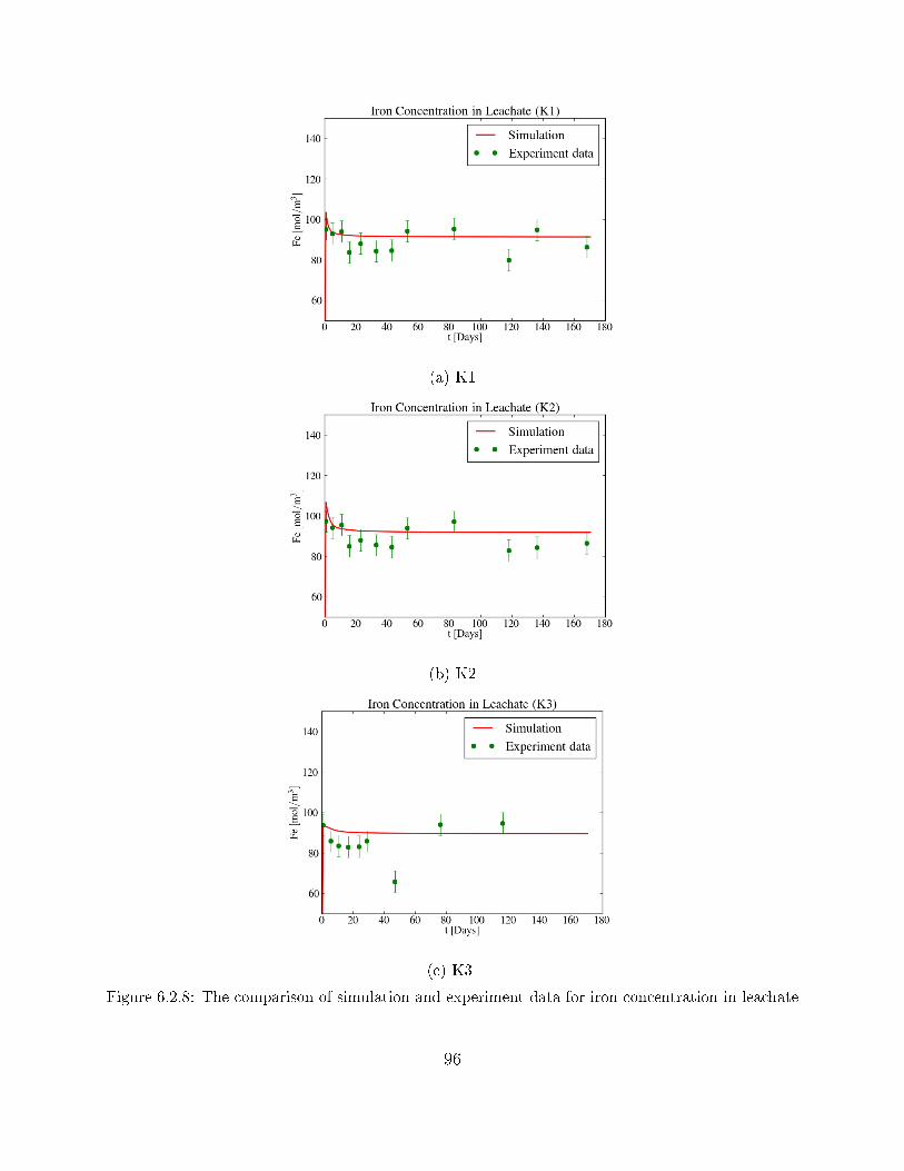
(a) K1

(b) K2

(c) K3

Figure 6.2.8: The comparison of simulation and experiment data for iron concentration in leachate

96

(a) K1

(b) K2

(c) K3

Figure 6.2.9: The comparison of simulation and experiment data for pH of leachate

97

except for the pH and iron concentrations which uctuated markedly in the experiments and

our model can not capture this uctuation. This may be due to the precipitation reactions

in our model which are assumed to be under constant precipitation rate or could simply be

experimental inaccuracy. The jump in the concentrations of iron, pH and Eh around day 35,

which can be observed in experiment K3, was due to experimental problems. The feed to the

column was stopped for a month and, while this period is ignored in the leach time, reactions

will still have continued over this one month period, albeit at a much slower rate. Due to

the lack of alternative experimental data, K3 is still used to provide a reference for validation.

6.2.3 Verication for Two Phase Heat Transfer

To verify the code for the coupled two phase heat transfer model, the method of man-

ufactured solutions (MMS) is used, as there is a lack of appropriate experimental data or

analytical solutions. The MMS can provide an approach to generate a non-trivial analytical

solution for code verication when a reliable exact solution for the model does not exist.

The analytical solution of the MMS need not be physically realistic and the code is veried

in a purely mathematical way [129].

Firstly, considering a simple 1-D case, we can rewrite the equations of two phase heat

transfer (Equation 3.2.13 and 3.2.15) as an operator of temperature, which is Equation

6.2.10. We assume that there is no immobile liquid or heat source/sink when verifying the

two phase heat transfer model.

L(Ts) ≡∂(Cpsρs(1− φ)Ts)

∂t+ heff (Ts − Tl) = 0 (6.2.10a)

L(Tl) ≡∂(θlTl)

∂t−∇ · (θlλl∇Tl) +∇ · (ulθlTl)−

heffCplρl

(Ts − Tl) = 0 (6.2.10b)

Then two arbitrary continuum solutions are chosen to be the analytical solutions for the

coupled liquid and solid heat transfer, those solutions can be independent of the model and

hosted equations, so that any solutions can be chosen [129]. The following two 1-D transient

solutions of Equation 6.2.11 are chosen for the liquid and rock temperature respectively. In

our case, the exponential and trigonometric functions are chosen because they have an innite

98

sum of terms when expanded as polynomials via Taylor expansion, although theoretically

any form of solutions can be chosen in MMS.

Ts = 303.16− exp (A1x) + cos (Bt) (6.2.11a)

Tl = 333.16− exp (A2x) + sin (Bt) (6.2.11b)

where,

A1 =1

x0

, (6.2.12a)

A2 =ulλlx0

, (6.2.12b)

B =1

2t0(6.2.12c)

The source terms Qs(t, x) and Ql(t, x) should be generated for the two coupled heat

transfer equation, adding the source terms to equations 6.2.10, the solutions that Ts(t, x) =

Ts(t, x), and Tl(t, x) = Tl(t, x) will be produced. The source term can be derived by operating

T with L:

Qs(t, x) = L(Ts(t, x))

=∂(Cpsρs(1− φ)Ts)

∂t+ heff (Ts − Tl)

= −B Cpsρs(1− φ) sin(Bt)

+ heff [−30− exp (A1x) + cos (Bt) + exp (A2x)− sin (Bt)]

(6.2.13a)

Ql(t, x) = L(Tl(t, x))

=∂(θlTl)


heffCplρl

(Ts − Tl)

= B θl cos (Bt) + A22 θlλl exp (A2x)− A2 · θlul · exp (A2x)

− heffCplρl

[−30− exp (A1x) + cos (Bt) + exp (A2x)− sin (Bt)]

(6.2.13b)

Finally, the source terms from Equation 6.2.13 are added to the hosted equations,

L(Ts) ≡∂(Cpsρs(1− φ)Ts)

∂t+ heff (Ts − Tl) = Qs(t, x) (6.2.14a)

L(Tl) ≡∂(θlTl)


heffCplρl

(Ts − Tl) = Ql(t, x) (6.2.14b)

99

If Equation 6.2.14 is now solved, it should return Equation 6.2.11 if the code is written

correctly.

The 1-D simulations have been tested with MMS for several mesh sizes and time steps.

The simulation set-ups and parameters are listed in Table 6.2. The meshes are discretized

into 10 to 800 elements, and time steps of 0.0625s to 2s are selected. The absolute errors of

simulated liquid and rock temperatures are calculated by comparison with their analytical

solutions (Equations 6.2.11).

Table 6.2: Simulation Conditions and Parameters

Parameter Value Unit

1-D ow and Column Geometry

Length (x0) 400 m

Porosity (φ) 0.4 -

Absolute permeability (K) 2.3× 10−9 m2/s

Darcy Flux (ul) 2.17× 10−6 m/s

Liquid

Saturation (Sl) 0.08226 -

Liquid hold-up (θl) 0.033 -

Density (ρl) 983 kg/m3

Heat Capacity (Cpl) 4.185 kJ/kg ·KLiquid Thermal Diusivity (λl) 5.5−7 kW/mk

Rock

Density (ρs) 1940 kg/m3

Heat Capacity (Cps) 0.8 kJ/(kg ·K)

Eective Heat transfer coecient (heff) 0.02 kW/(m3 ·K)

The l2-norm of the errors E are calculated using Equation 6.2.15. Plots of the l2-norm of of

the errors for liquid and rock temperatures along with temporal and spatial discretizations are

shown in Figure 6.2.10. It can be observed that both liquid and rock temperatures approach

to their analytical solutions as the temporal resolution is increased from ∆t = 2 to 0.0625s.

While the convergence of rock temperature is independent of the spatial discretization due

to the fact that the spatial heat conduction terms are neglected. The liquid temperature

100

converges with improving mesh resolution. Above a certain resolution there is a limit to

further decrease in the error as it is dominated by the error associated with the temporal

discretizations:

| E |=

√√√√ n∑ele=1

(Eele)2 (6.2.15)

(a) The l2-norm of the error for liquid

temperature.

(b) The l2-norm of the error for rock

temperature.

Figure 6.2.10: The l2-norm of the errors along with various temporal and spatial discretizations.

To further analyse the convergence, instead of l2-norm , the absolute errors (the dierence

between simulated value and the exact value) of each element of the column are analysed

for both temporal and spatial discretization. When analysing temporal discretization error,

the temporal resolution is varied with the xed ne mesh of 800 elements, which is shown

in Figure 6.2.11, for spatial discretization. When analysing spatial discretization, the mesh

resolution is varied with the time step being xed to be ∆t = 0.0625s, which is shown in

Figure 6.2.12. These plots shows similar behaviour and support the observed results of plots

6.2.10. For the time discretization, the absolute errors of both liquid and rock tempera-

tures for all the elements are reduced by reducing the time step, and those errors are almost

constant along the column for each time step, which is illustrated in Figure 6.2.11(a) and

6.2.11(b). Figure 6.2.11(c) and 6.2.11(d) show that the absolute error of liquid temperature

of an individual element is almost constant along simulation time, while the absolute errors

of rock phase temperature is slightly increasing with simulation time.

101

(a) The absolute errors for liquid tem-

perature along the length of column

when t=1000s.

(b) The absolute errors for rock temper-

ature along the length of column when

t=1000s.

(c) The absolute errors for liquid tem-

perature in the middle of the column

(x=200) along simulation time.

(d) The absolute errors for rock tem-

perature in the middle of the column

(x=200) along simulation time.

Figure 6.2.11: Convergence analysis for temporal discretization with 800 mesh elements, the plot of

absolute errors for time steps of 2,1,0.5,0.25,0.125 and 0.0625s

102

(a) The absolute errors for liquid temperature along the

length of column when t=1000s.

(b) The absolute errors for rock temperature along the

length of column when t=1000s.

103

(c) The absolute errors for liquid temperature in the middle

of the column (x=200) along simulation time.

(d) The absolute errors for rock temperature in the middle

of the column (x=200) along simulation time.

Figure 6.2.12: Convergence analysis for spatial discretization with ∆t = 0.0625s, the plot of absolute

errors for mesh with 10, 25, 50, 100, 200, 400, 800 elements.

For mesh discretization, Figure 6.2.12(a) and 6.2.12(c) show that the absolute errors for

liquid temperature with ne meshes converges to a small values and the further reduction

of the errors by rening the mesh is signicantly retarded, which coincides with the plot

104

6.2.10(a). Furthermore, the absolute errors of both liquid and rock temperatures increase

along the column with a signicant increase near the end of the column, but this phenomena

is improved by rening the mesh. Figures 6.2.12(d) and 6.2.12(b) demonstrate the conclusion

that the absolute errors of rock temperature is almost independent of the mesh discretiza-

tion, and that they increase with simulation time. The order of convergence is calculated and

ploted in Figure 6.2.13 for time, and Figure 6.2.14 for space. As is expected, Figure 6.2.14(b)

shows that the convergence of the rock temperature is independent of the space resolution

with an order of zero. The liquid temperature is approximately rst order accurate in both

time and space, which is consistent with what is expected from a control volume method.

From this analysis it has been shown that the heat transfer models are well behaved as im-

plemented and exhibit rst order spatial and temporal convergence, as expected for a nite

volume based method. The exception is the rock temperature, which does not converge with

changes in spatial resolution, though it does with temporal resolution. This is because solid

phase heat conduction is not included in the model and there are thus no spatial derivatives

in rock temperature.

(a) The order of convergence for tempo-

ral discretization of liquid temperature.

(b) The order of convergence for tempo-

ral discretization of rock temperature.

Figure 6.2.13: The order of convergence for temporal discretization, with the mesh of 800 elements.

105

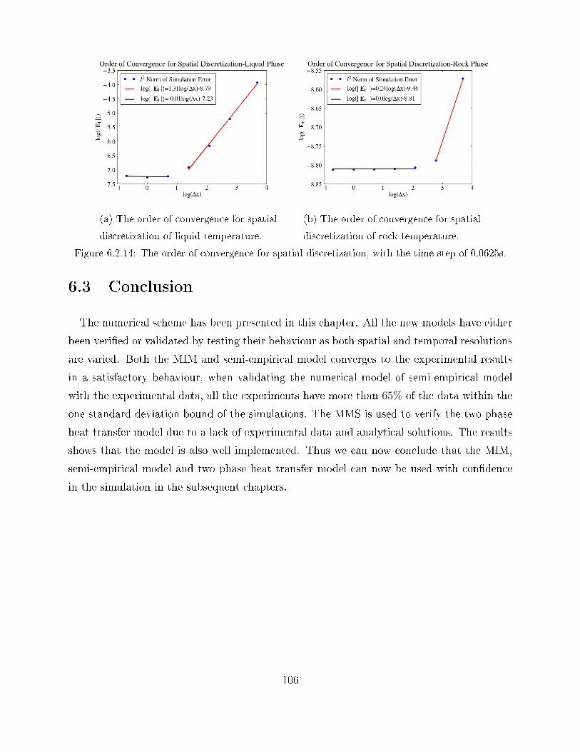
(a) The order of convergence for spatial

discretization of liquid temperature.

(b) The order of convergence for spatial

discretization of rock temperature.

Figure 6.2.14: The order of convergence for spatial discretization, with the time step of 0.0625s.

6.3 Conclusion

The numerical scheme has been presented in this chapter. All the new models have either

been veried or validated by testing their behaviour as both spatial and temporal resolutions

are varied. Both the MIM and semi-empirical model converges to the experimental results

in a satisfactory behaviour, when validating the numerical model of semi-empirical model

with the experimental data, all the experiments have more than 65% of the data within the

one standard deviation bound of the simulations. The MMS is used to verify the two phase

heat transfer model due to a lack of experimental data and analytical solutions. The results

shows that the model is also well implemented. Thus we can now conclude that the MIM,

semi-empirical model and two phase heat transfer model can now be used with condence

in the simulation in the subsequent chapters.

106

Chapter 7

1D Simulations and Sensitivity Analysis

In order to design an ecient heap, it is essential to investigate the extent to which

dierent factors will inuence the leaching. In this chapter, Some 1D simulations have been

implemented to analyse the following factors on chalcopyrite heap leaching: the bacteria

eect, the eect of immobile liquid, the solution temperature, and the solution concentration

including Fe3+ and pH.

7.1 Model Description-1D

Five sets of 1D models with dierent solution or geometry conditions have been carried

out to analyse the leaching performance under dierent conditions. Firstly, the eects of

bacteria and mobile-immobile liquid are investigated. Then, the dierent conditions of solu-

tion temperature and concentrations are analysed separately. All these models are compared

with a base model which does not include the MIM and bacterial eects. The common pa-

rameters set for all these models and the boundary and initial conditions of the base model

are listed in Table 7.1. The conditions of bacteria applied to the bioleaching model are listed

in Table 7.2, these parameters are from the bacteria leaching model presented by Leahy et

al. (2007) [85]. The conditions of the other sets of models for sensitivity analysis of dierent

solution conditions are listed in Table 7.3. All the mass and heat boundary conditions are

applied from the top of the heap, with zero gradient conditions applied at the bottom.

107

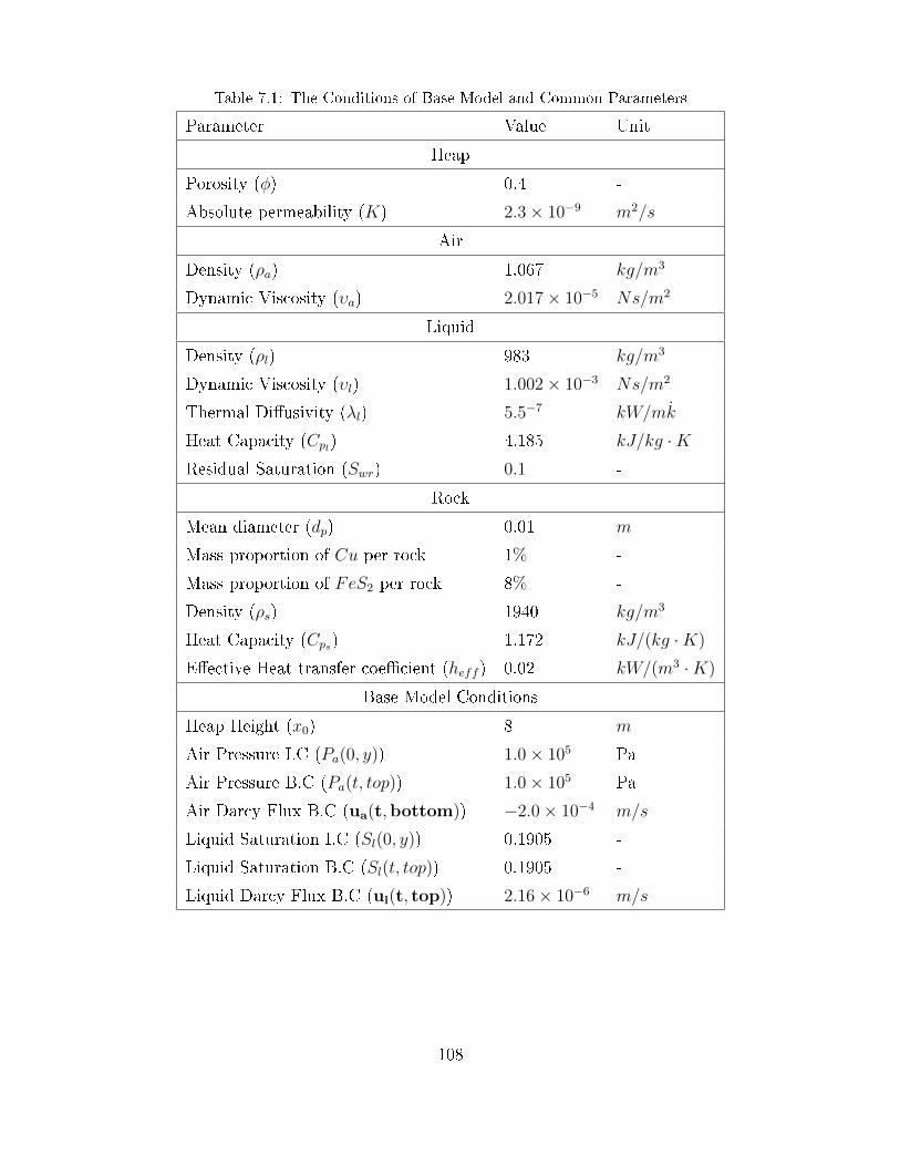
Table 7.1: The Conditions of Base Model and Common Parameters


Heap

Porosity (φ) 0.4 -


Air

Density (ρa) 1.067 kg/m3

Dynamic Viscosity (υa) 2.017× 10−5 Ns/m2

Liquid


Dynamic Viscosity (υl) 1.002× 10−3 Ns/m2

Thermal Diusivity (λl) 5.5−7 kW/mk

Heat Capacity (Cpl) 4.185 kJ/kg ·KResidual Saturation (Swr) 0.1 -

Rock

Mean diameter (dp) 0.01 m

Mass proportion of Cu per rock 1% -

Mass proportion of FeS2 per rock 8% -



Eective Heat transfer coecient (heff ) 0.02 kW/(m3 ·K)

Base Model Conditions

Heap Height (x0) 8 m

Air Pressure I.C (Pa(0, y)) 1.0× 105 Pa

Air Pressure B.C (Pa(t, top)) 1.0× 105 Pa

Air Darcy Flux B.C (ua(t,bottom)) −2.0× 10−4 m/s

Liquid Saturation I.C (Sl(0, y)) 0.1905 -

Liquid Saturation B.C (Sl(t, top)) 0.1905 -

Liquid Darcy Flux B.C (ul(t, top)) 2.16× 10−6 m/s

108

Table 7.2: Parameters and Conditions for Bacteria Leaching

Parameters

Y 3.7× 1013 cells(kg Fe2+ consumed)−1

KM,O 1.6× 10−3 kg m−1

KM,Fe2+ 5.58× 10−3 kg m−1

Mesophiles

k1 7.1× 10−5 s−1

k2 4.0× 10−7 s−1

kdeath 3.5× 10−6 s−1

ψmax 7.8× 1012 cells(kg ore)−1

µmax 3.0× 10−5 s−1

Tshift 0.0 C

Moderate Thermophiles

k1 7.1× 10−5 s−1

k2 4.0× 10−7 s−1

kdeath 4.0× 10−6 s−1

ψmax 7.8× 1012 cells(kg ore)−1

µmax 2.5× 10−5 s−1

Tshift 8.0 C

Initial and boundary conditions for both bacteria

ψ(0, y) 0 cells(kg ore)−1

φ(0, y) 0.5× 1014 cells(m3 liquid)−1

φ(t, top) 0 cells(m3 liquid)−1

Table 7.3: The Parameters and their respective values used in the sensitivity study

Parameter Lower Base Higher Unit

pH(t, top) 0.6 1.2 2.4 mol/m3

CFe3+(t, top) 9 18 36 mol/m3

Tl(t, top) 12.5 25 50 C

109

7.2 The Eect of Bacteria

To investigate the bacteria-temperature dependence, and their eect on leaching eciency,

two bacterial populations are considered in the bioleaching model, which are mesophiles (op-

timal temperature is 37.65C) and moderate thermophiles (optimal temperature is 45.65C)

and their parameters are listed in Table 7.2. The algorithm of the bio-leaching model and

the explanation of the parameters are described in Section 3.3.2 in Chapter 3.

As is illustrated in Figure 7.2.1(a), the average copper extraction of the heap with bacteria

is signicantly higher than the base case without any bacteria. This is in agreement with

what is observed in industry where bacterial action is a critical factor in sulphide leaching.

As is shown in Figures 7.2.3, the rock and liquid temperature of bioleaching is much higher

than the base case, since both mesophiles and moderate thermophiles promote ferrous oxi-

dation which will release large amounts of heat. Ferrous oxidation in bioleaching accounts

for a signicant part of the total heat production in the heap, while in the base model, the

reaction of ferrous oxidation is so slow that the heat released by it can be neglected (Figure

7.2.2). As the result of higher ferrous oxidation rate in bioleaching, the average concentra-

tion of Fe3+ in the bacteria case is much higher than that in the base model (Figure 7.2.3(c)).

The dissolution of sulphides, especially the pyrite, results in acid production, which ac-

counts for a lower outlet pH in the bio-leaching simulation. A disadvantage of the increased

leaching and ferrous oxidation rate is that the increased Fe3+ encourages the formation of

jarosite (Figure 7.2.3(e) and 7.2.3(f)). In the real system these precipitates have been impli-

cated in passivation of the mineral surfaces, though this eect is not well understood and the

phenomenon is not included in the current modelling. On the other side, the encouragement

of the jarosite precipitation can produce acid and lower the pH, which is benecial to copper

leaching.

Obviously, all the phenomena discussed above in bioleaching, which include increased heap

temperature, increased Fe3+, decreased pH are benecial for leaching copper from the rock,

which can be easily derived from the kinetic rate equation for chalcopyrite dissolution in

Table 3.1 in Chapter 3. Because we assume the non-accumulation of elemental sulphur, the

110

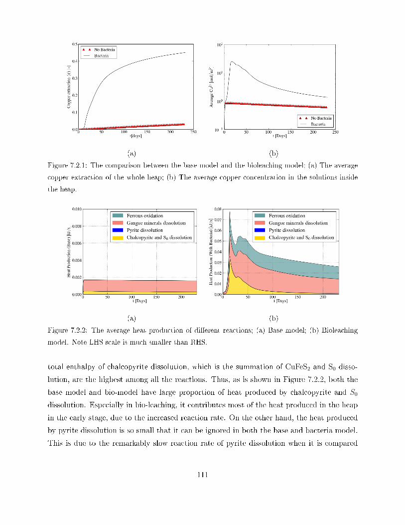
(a) (b)

Figure 7.2.1: The comparison between the base model and the bioleaching model; (a) The average

copper extraction of the whole heap; (b) The average copper concentration in the solutions inside

the heap.

(a) (b)

Figure 7.2.2: The average heat production of dierent reactions; (a) Base model; (b) Bioleaching

model. Note LHS scale is much smaller than RHS.

total enthalpy of chalcopyrite dissolution, which is the summation of CuFeS2 and S0 disso-

lution, are the highest among all the reactions. Thus, as is shown in Figure 7.2.2, both the

base model and bio-model have large proportion of heat produced by chalcopyrite and S0

dissolution. Especially in bio-leaching, it contributes most of the heat produced in the heap

in the early stage, due to the increased reaction rate. On the other hand, the heat produced

by pyrite dissolution is so small that it can be ignored in both the base and bacteria model.

This is due to the remarkably slow reaction rate of pyrite dissolution when it is compared

111

(a) (b)

(c) (d)

(e) (f)

Figure 7.2.3: The comparison between the base model and the bioleaching model; (a) Average rock

and liquid temperature of the whole heap; (b) Average bacteria population in the liquid; (c) Average

ferric concentration in the heap; (d) Average ferrous concentration in the heap; (e) Average pH in

the heap; (f) Average copper concentration in the heap.

112

with the other reaction. In the real system, though, the bacterial leaching can also promote

the pyrite dissolution rate and thus produce more ferric ions that leach the copper. In our

current model, the eect of bacteria on pyrite leaching is neglected and only the bacterial

eect on ferrous oxidation is considered, though this would be a topic for future work.

The gangue minerals also produce signicant heat in both the base and bacteria case,

especially when the other reactions are slow. However, due to our initial assumption that

the gangue minerals are dissolving at a constant rate based on the pH (Table 3.1 in Chapter

3), the high heat production from dissolving the gangue mineral might need to be calibrated

more accurately against experiment.

The average copper concentration in solutions for the bacteria leaching reaches a peak

after about 20 days of leaching, and then it drops. It can be observed that the time that

peak copper concentration occurs coincides with the time that the average heap tempera-

ture reached around 38C, which is the optimal temperature for the mesophiles. Also, the

population of mesophiles and Fe3+ concentration in liquid reach their rst peak, and the pH

of liquid reaches its rst nadir around the same time (near the 20th day). After that time,

Fe3+ concentrations and the acidity of the liquid drops slightly as the temperature is keeping

increasing and shifting far from the optimal point for the mesophiles. The dropping of Fe3+

concentrations and the acidity of the solution is relieved when the temperature is increasing

towards the optimal point of moderate thermophiles, and then Fe3+ concentrations and the

acidity starts increasing again when the leaching runs for around 30 days when the tem-

perature reached around 44C, which means the moderate thermophiles have the optimal

activity and their populations have grown to the peak value.

When the leaching time passed 50 days, where the average copper extraction achieved 0.3

in the bioleaching model, the copper extraction rate is further decreasing. This is due to

the reduced accessibility of mineral grains inside the ore as the extraction continues, Figure

5.3.1 in Chapter 5 shows the apparent kinetics of copper leaching as a function of extraction,

and it indicates that the extraction rate decreases as the extracton increases. The heap

temperature also starts to drop around the same time, with the average temperature having

reached a maximum of around 47C. Since the total enthalpy released by dissolving the

113

chalcopyrite is the highest of the reactions we considered in our model, the decreasing of

the copper dissolution can reduce the heat generated in leaching, and thus the increasing of

temperature is stopped when the dissolution rate decreased to a certain point. The decreas-

ing of temperature favours mesophiles and makes the population of moderate thermophiles

decrease. As is shown in Figure 7.2.3(a) , the average heap temperatures after 90 days lies

within the range of 40C to 34C, which make the mesophiles more active than moderate

thermophiles, and the bacteria population illustrated in 7.2.3(b) agrees with this suggestion.

Due to the decreasing leaching rate and temperature, the average Fe2+ concentrations are

reduced as is illustrated in Figure 7.2.3(d), and this results in a slower ferrous oxidation rate

and decreasing Fe3+ concentrations and the acidity of the liquid.

To further analyse the leaching behaviour, the propagation of solutes, temperature, bacte-

ria and the evolution of copper extraction along the heap height are shown in Figures 7.2.4,

where the height is the distance from the bottom. For the rst 50 days, the chalcopyrite

extraction is increasing remarkably throughout the heap, especially the middle and lower

part of the heap as is shown in Figure 7.2.4(a). This agrees with the sharp slope of average

copper extraction for the rst 50 days illustrated in Figure 7.2.1(a). This is due to the

signicant rise in the heap temperature for the lower bottom part (Figure 7.2.4(b)). Both

of the bacteria are initially uniform inside the heap, and the distribution of their population

start to change when the temperature distribution of the heap varies. As is shown in Figure

7.2.4(e), the mesophiles population from the top to the middle of the heap rise quickly for

the rst 50 days due to the favourable temperature evolution, which increased from 25C to

45C. When the temperature further rises from the middle to the bottom part with time,

the temperature become unfavourable to mesophiles, and thus the mesophiles population

decrease noticeably from the middle to the bottom of the heap, especially on the 50th day,

when the bottom temperature is as high as 70C.

The behaviour of Fe3+ concentration (Figure 7.2.4(c)) and Fe2+ concentration (Figure

7.2.4(d)) across the heap also correspond to the bacteria and temperature evolution. The

Fe3+ concentration is much higher from the top to the middle of the heap, and the con-

centration rises with time for the rst 50 days. On the other side the Fe2+ concentration

is lower from the top to the middle of the heap, and further decreases with time, which exactly

114

(a) (b)

(c) (d)

(e) (f)

115

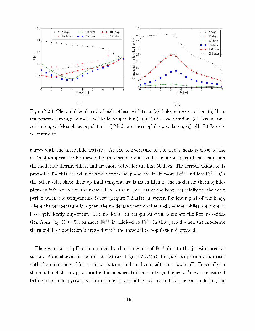
(g) (h)

Figure 7.2.4: The variables along the height of heap with time; (a) chalcopyrite extraction; (b) Heap

temperature (average of rock and liquid temperature); (c) Ferric concentration; (d) Ferrous con-

centration; (e) Mesophiles population; (f) Moderate thermophiles population; (g) pH; (h) Jarosite

concentration.

agrees with the mesophile activity. As the temperature of the upper heap is close to the

optimal temperature for mesophile, they are more active in the upper part of the heap than

the moderate thermophiles, and are more active for the rst 50 days. The ferrous oxidation is

promoted for this period in this part of the heap and results in more Fe3+ and less Fe2+. On

the other side, since their optimal temperature is much higher, the moderate thermophiles

plays an inferior role to the mesophiles in the upper part of the heap, especially for the early

period when the temperature is low (Figure 7.2.4(f)), however, for lower part of the heap,

where the temperature is higher, the moderate thermophiles and the mesophiles are more or

less equivalently important. The moderate thermophiles even dominate the ferrous oxida-

tion from day 30 to 50, as more Fe2+ is oxidised to Fe3+ in this period when the moderate

thermophiles population increased while the mesophiles population decreased.

The evolution of pH is dominated by the behaviour of Fe3+ due to the jarosite precipi-

tation. As is shown in Figure 7.2.4(g) and Figure 7.2.4(h), the jarosite precipitation rises

with the increasing of ferric concentration, and further results in a lower pH. Especially in

the middle of the heap, where the ferric concentration is always highest. As was mentioned

before, the chalcopyrite dissolution kinetics are inuenced by multiple factors including the

116

Fe3+ concentration, pH and temperature. The dissolution rate is decided by the superposi-

tion of these eects and thus the middle, around the 3rd meter of the heap has the highest

extraction for the rst 100 days, since at that position, the balance of the ferric, pH and

te,mperature favours the extraction rate. For example, although the temperature is highest

near the bottom of the heap, which can increase the dissolution rate, the Fe3+ and H+ con-

centration there is low.

Beyond 100 days, the heap temperature starts to decrease as can be seen from Figure

7.2.4(b), which is probably due to the depletion of the mineral which is easier to access (e.g.

near the surface) as it is suggested in the previous discussion. Around 231 days, the copper

extraction is dominated by the bottom of the heap (Figure 7.2.4(a)) rather than the middle

part. This is because the initially high Fe3+ and H+ concentration in the middle of the heap

decreases after 100 days, which results in a more uniform ferric distribution throughout the

heap, so the domination of copper dissolution after 100 days is then under the high temper-

ature near the heap bottom.

7.3 The Eect of MIM

As is illustrated in Figure 7.3.1(a) and 7.3.1(b), the copper extraction rate and the cop-

per concentration of the model using conventional advection-dispersion equation (ADE) is

higher than those using mobile immobile model (MIM), which indicates that the stagnant

liquid inside the porous heap may slow the copper extraction rate. The overall dissolution

rate is slow. This is because the low applied solution temperature and the slow ferrous ox-

idation rate due to the assumption of neglecting the bacterial activity. The heap could not

be warmed up due to the slow reaction rates, and the heat generation rate by the reactions

are much slower than the transport rate of the cold solution through the heap.

The curve of chalcopyrite extraction for both models are linear with time (Figure 7.3.1(a) )

is reviewed in Section 2.3.3 of Chapter 2 the linear curve suggests the chalcopyrite dissolution

is under surface reaction control. The reaction control indicates the transport of solution

is much faster than the consumption of solution by chemical reactions, so the dissolution

117

(a) (b)

Figure 7.3.1: The comparison between the base model and the bioleaching model; (a) The average

copper extraction of the whole heap; (b) The average copper concentration in the solutions inside

the heap.

kinetics is governed by the reaction kinetic rate equations listed in the Table 3.1 in Chapter

3. Thus the solution concentrations around the rock are the critical factors that decide the

extraction rates. As is listed in the Table 3.1, chalcopyrite dissolution rate positively corre-

lates to the H+ and Fe3+ concentrations, and the reaction order with respect to H+ and Fe3+

are 0.8 and 0.42 respectively, which means that the H+ concentration aects the dissolution

rate more than Fe3+ concentration.

By observing the average concentrations of H+ and Fe3+ in Figures 7.3.2(d) and 7.3.2(b), it

can be seen that the pH of conventional ADE is much lower than that of MIM, and the Fe3+

concentration of conventional ADE is slightly lower than that of MIM. This is mainly due to

the faster copper dissolution rate of conventional ADE will produce signicant acid by the

total reaction of Equations 3.3.1 and 3.3.2, also, the net heat consumption and generation

of these two dissolution reactions can produce signicant heat, therefore the average tem-

perature of the conventional model are higher than the MIM (7.3.2(a)), which also further

increased the reaction rate of conventional model. Furthermore, the lower dissolution rate

of MIM leads to a slower depletion of Fe3+ concentration. Also, although more Fe2+ concen-

trations are produced by the dissolution reactions of conventional model, most of them are

unable to be converted to Fe3+ due to the slow ferrous oxidation reaction. Thus, the faster

Fe3+ consumption rate and slower ferrous oxidation rate makes the Fe2+ concentrations are

118

(a) (b)

(c) (d)

(e)

Figure 7.3.2: The comparison between the conventional ADE model and the MIM; (a) Average rock

and liquid temperature of the whole heap; (b) Average ferric concentration in the heap; (c) Average

ferrous concentration in the heap; (d) Average pH in the heap; (e) Average copper concentration in

the heap.

119

much higher in the conventional ADE model, and its Fe3+ concentrations are slightly lower.

Less jarosite is thus precipitated in the conventional ADE due to the low pH and Fe3+ con-

centration, which is illustrated in Figure 7.3.2(e).

In additional to the faster dissolution rate of the conventional ADE model producing more

H+, another more intrinsic reason that make the MIM have a higher pH is that the existence

of the stagnant liquid will dilute the average concentrations of the solution. Although the

applied concentrations, supercial velocity, volume ow rate and total liquid hold-up are

exactly the same for both models, the actual mobile liquid hold-up of the MIM is less than

that of the conventional ADE. As is described in Equation 3.2.8, under the same darcy ux,

the actual advection velocity of MIM is faster with a lower dynamic liquid hold-up. Although

the concentrations of reactants (Fe+ and H+) applied from the heap top and the total liquid

hold-up inside the heap are the same for both models, the concentration of each reactant in

the stagnant liquid is much smaller than that in the dynamic liquid when using MIM. Thus,

the lower concentration of H+ in the immobile region dilutes the concentrations in mobile

liquid, and thus lowers the average concentrations in the total liquid hold-up when using

MIM, while the average concentrations in the total liquid hold-up when using conventional

model are the same with those in the dynamic liquid. Therefore, this leads to a higher pH

and slower copper dissolution rates when using MIM, then the slower copper dissolution

rates further leads to a lower production of acid, which result in a much higher pH of the

MIM than the conventional ADE (Figure 7.3.2(d)).

The further evidence that the immobile liquid will dilute the H+ concentration of heap

are shown in Figure 7.3.3(f), the pH of immobile region is always higher than that of the

mobile liquid from the heap top (length=8m) to the bottom (length=0m) throughout the

whole leaching period, causing the mean pH of the mobile and immobile liquid to always be

lower than that in the dynamic liquid. The mean pH illustrated in Figure 7.3.3(e) shows

that the H+ concentration is reducing from top to the bottom. This suggests that when

the solution is propagating along the heap the H+ concentration is consumed by a domi-

nant reaction, probably the ferrous oxidation reaction of Equation 3.3.5. This results in a

slower copper extraction rate from the bottom half of the heap, which is shown in Figure

7.3.3(a). The kinetic equation for ferrous oxidation in Table 3.1 suggests that the oxidation

120

(a) (b)

(c) (d)

(e) (f)

Figure 7.3.3: The variables along the height of heap with time of the MIM, (the concentrations

are based on the mean of the mobile and immobile value); (a) Chalcopyrite extraction; (b) Average

copper concentration inside the heap; (c) Average dierence between the mobile and immobile

copper concentration; (d) Average concentration of jarosite inside the heap; (e) Average pH inside

the heap; (f) The average dierence between the mobile and immobile pH.

121

rate is positively dependent on Fe2+ but negatively dependent on H+ concentration. Figures

7.3.3(e) and 7.3.4(a) shows that the Fe2+ concentration is increasing and H+ concentration

is decreasing along the heap, which cause the oxidation rate to rise along the heap, therefore

more H+ ions are consumed. On the other hand, the jarosite precipitation in Figure 7.3.3(d)

is much faster in the top half of the heap, which can make up for the H+ concentration loss.

Like H+ concentration, Fe3+ concentration shown in Figure 7.3.4(c) is consumed and re-

duces along the heap, and with both varying slightly with time. The slow chemical reactions

inside the heap lead the change of the mass to equilibrium and mass transport achieves

steady state quickly. By comparing the dierence of the mobile immobile eld, both of the

mobile H+ and Fe3+ concentrations are slightly higher than their immobile eld, which is

illustrated in Figures 7.3.3(f) and 7.3.4(d). As is shown in Figure 7.3.1(a), the coper dissolu-

tion rate is almost constant but with a slightly decreasing trend along the time, the reducing

of the chemical reaction rates then relief the reactant consumption and make the H+ and

Fe3+ concentration slightly increased with time, this suggestion can be support by Figure

7.3.4(c), Figure 7.3.3(e), Figure 7.3.2(b) and Figure 7.3.2(d). As the immobile liquid plays a

role in reducing the mass transport rate, the immobile concentrations always lag temporally

behind the mobile concentration, thus the reducing mass consumption of H+ and Fe3+ leads

the mobile mass more advanced. Furthermore, since the mass consumption of H+ and Fe3+

are more signicant in the top half of the heap, more H+ and Fe3+ ions are consumed in this

region. Since the solution is applied from the top, the chemical consumptions of the upper

heap are recharged quickly, so the mobile concentrations and their gradients are steepest

near the top. Therefore, the dierence between the mobile and immobile concentrations are

more in the upper heap due to the temporal lag.

The Cu2+, Fe2+ and temperature are generated by the net reactions, as is shown in Figure

7.3.3(b), Figure 7.3.4(a) and Figure 7.3.4(e), all of them increases along the heap with a

decreasing rate. The temperature and Cu2+ concentration rstly increased with the initial

reactions, where the wave of the mass that propagated down the heap can be observed for

the initial leaching period, and the Cu2+ concentration achieved a steady spacial distribution

quickly. Then the overall concentrations started to decrease after mass propagation wave

passed the heap bottom, and the spacial concentration dissolution became steady. Since the

122

(a) (b)

(c) (d)

(e) (f)

Figure 7.3.4: The variables along the height of heap with time of the MIM, (the concentrations are

based on the mean of the mobile and immobile value); (a) Average ferrous concentration inside the

heap; (b) Average dierence between the mobile and immobile ferrous concentration; (c) Average

ferric concentration inside the heap; (d) Average dierence between the mobile and immobile ferric

concentration; (e) Average temperature inside the heap; (f) Average dierence between the mobile

and immobile temperature.

123

temporal lag of the immobile concentrations, the mobile temperature and copper concentra-

tions are much more than their immobile mass, especially near the wave front of the mass

propagation, when the leaching is before 30 days for temperature (Figure 7.3.4(f)) and before

5 days for Cu2+ (Figure 7.3.3(c)). When the overall concentrations started to reduce, the

temporal lag leads the immobile mass more than the mobile eld, which are shown in Figure

7.3.4(b) for Fe2+, Figure 7.3.3(c) for Cu2+ after 5 days, and Figure 7.3.4(f) for temperature

after 30 days.

As is discussed above, the neglecting of the stagnant liquid in heap leaching simulation can

cause errors in predictions of ether extractions or concentrations. Being dierent from the

sensitivity analysis presented in the following sections, which only evaluates the eects of dif-

ferent parameters on leaching behaviour, the analysis of the MIM evaluates the inaccuracies

accompanied with the model when using traditional ADE and determines the importance of

the inuence of the stagnant zones on the leaching performance. Thus, we can conclude that

it is necessary to replace the conventional ADE with the MIM in heap leaching modelling to

improve the accuracy, while in all the previous studies available in literature the conventional

ADE were applied to the sulphides heap leaching modelling.

7.4 Sensitivity Analysis

In heap leaching, various factors can inuence the performance of the system. Thus, it

is desirable to carry out the sensitivity analysis to evaluate how important each parameter

can aect the leaching. The results of sensitivity analysis is useful for optimizing the heap

operations.

7.4.1 The Eect of Solution Temperature

In this model, the initial temperature of the heap is kept to be 25 C, while the temper-

ature of the solution applied from the top are varied to be 12.5 C for a lower case, and 50C for a higher case. The results listed in Figure 7.4.1(a) shows that increasing the tem-

perature can improve the copper extraction rate, and thus a higher copper concentration

in the solutions(Figure 7.4.1(b) ). But due to the absence of bacterial activity, the overall

124

(a) (b)

(c)

Figure 7.4.1: Comparing the models with three dierent solution temperature applied from heap top;

(a) Chalcopyrite extraction; (b) Average copper concentration in the heap; (c) Average temperature

of the heap.

copper extraction of the three cases are low. It can be seen from Figure 7.4.1(c) that the

temperature of the solution in the high temperature case is only increased by around 2 C

by the heat produced by the chemical reactions even though the overall reaction rates are

increased due to the higher temperature.

Figure 7.4.3(c) of the ferrous oxidation rates shows that the oxidation rates were signi-

cantly increased by the higher temperature of 50 C. This is because in the reaction kinetic

125

of ferrous oxidation (listed in Table 3.1), the activation energy of the oxidation without the

bacterial eect is high and so the oxidation rate is very sensitive to temperature changes.

However, although the high solution temperature improves the ferrous oxidation rate, the

rate is still slow when it is compared with the chalcopyrite dissolution rate, which has a much

smaller activation energy. Thus most of the Fe2+ produced by the chalcopyrite dissolution

could not be oxidised to Fe3+, but accumulated in the solution, especially for the high tem-

perature case, which is illustrated in Figure 7.4.3(a). The increase of the copper extraction

results in a much higher Fe2+ concentration in the solution.

Since the chalcopyrite dissolution rates are much higher than the ferrous oxidation rates

for the high temperature case, the Fe3+ consumption rates are much faster than the genera-

tion rates, thus the amount of Fe3+ inside heap is much smaller for the high temperature case

than the other lower temperature cases, which are shown in Figure 7.4.3(b). The excess Fe3+

in the low temperature cases precipitated into jarosite, though in these simulation this could

be due to the speed of precipitation being simplied to be a constant rate which dependents

on the Fe3+ concentration. This also results in a high H+ concentration and low pH for the

low temperature models (Figure 7.4.2(a)), since the jarosite precipitation rate can release

large amounts of acid.

(a) (b)

Figure 7.4.2: Comparing the models with three dierent temperature; (a) Average pH in the heap;

(b) Average jarosite concentration in the heap.

126

(a)

(b)

(c)

Figure 7.4.3: Comparing the models with three dierent temperature; (a) Average ferrous concen-

tration in the heap; (b) Average ferric concentration in the heap; (c) Average ferrous oxidation

rate.127

(a)

(b)

128

(c)

(d)

Figure 7.4.4: The comparison of the variables between to high temperature and low temperature;

(a) Copper extraction; (b) Copper concentration; (c) Heap temperature; (d) pH.

129

(a)

(b)

130

(c)

(d)

Figure 7.4.5: The comparison of the variables between to high temperature and low temperature; (a)

Ferrous concentration; (b) Ferric concentration; (c) Ferrous oxidation rate; (d) The concentration

of jarosite.

131

The detail of spatial change of the species for the high and low temperature cases are

shown in Figures 7.4.4 and 7.4.5. It shows that both the temporal and spatial changes of

solution concentrations and copper extractions are more signicant with higher tempera-

tures. The highest copper extraction, which is illustrated in Figure 7.4.4(a), are near the

heap top for both the high and low temperature cases, which is reasonable because the solute

concentration of Fe3+ and H+ are highest when the solutions are applied from the top. The

temperatures of both cases are relatively uniform along the heap after 50 days, and remained

temporally unchanged. This is because the low reaction rate and thus low heat gains inside

the heap due to the absence of bacteria, and the temperature proles settled down quickly.

For the initial 30 days, the copper extraction simply decrease with depth for the high

temperature case, however, with the propagation of solution, the extraction near the bot-

tom started to increase after 50 days, while the extraction for the low temperature case was

just monotonously decreasing with depth for the whole leaching time. According to Figure

7.4.5(b), the increase in the copper extraction for the high temperature case near the heap

bottom was caused by the rise in the Fe3+ concentration in this region, which is resulted by

a faster ferrous oxidation rate around the bottom. It can be seen that the Fe3+ concentra-

tion initially decreased with depth as it was consumed by the chalcopyrite dissolution and

jarosite precipitation. On the other side, the Fe2+ concentration increased signicantly with

depth due the chalcopyrite dissolution, which has a positive eect on the ferrous oxidation

rate according to it's rate kinetic equation. When the Fe2+ concentration increased to a

certain point around the heap height of 5 meter (Figure 7.4.5(a)), the ferrous oxidation rate

surpassed the chalcopyrite dissolution rate and thus the Fe3+ concentration increased over

this lower portion of the heap.

7.4.2 The Eect of Fe3+ and pH

To evaluate the eects of leaching solutions, two sensitivity analysis have been separately

carried out for pH and Fe3+ concentrations, and they are compared with the same base case.

In these models, the applied pH and Fe3+ concentrations from the heap top are either halved

or doubled. Then both the temporal and spatial evolutions of chalcopyrite extraction, mass

and temperature for these ve dierent models (high and low Fe3+ concentrations, high and

132

low pH, and base case) are compared and shown in the following gures.

From Figure 7.4.6, it can be observed that either halving the pH or doubling the Fe3+ con-

centrations can increase the overall copper extractions within 231 days leaching to a similar

extent, while by halving the Fe3+ concentrations or doubling the pH the extraction can be

reduced to a similar extent. Which indicates that the copper extraction rate in our model

is similar sensitive to Fe3+ and pH. In our kinetic model of chalcopyrite which is listed in

Table 3.1, the chalcopyrite dissolution rate is 0.8 order with respect to H+ concentration and

0.42 order with respect to Fe3+ concentration, which means the dissolution rate itself should

be more sensitive to the change of pH than Fe3+ according to the rate equation. To further

examine extraction variations along the heap, the spatial distributions of copper extraction

are listed in Figure 7.4.6(b). The two optimum cases where the pH is halved or the Fe3+

concentration is doubled are compared together. It can be seen that the extraction decreases

more from top to bottom for the low pH case. At the top where the solutions are applied,

more copper is extracted in the low pH case than the high Fe3+ case, which agrees with

the kinetic equation used in our model. However, the extraction of the low pH model drops

faster with depth and thus results in a lower extraction near the heap bottom in the low pH

model than that in the high Fe3+ model. Therefore, the total extractions of the whole heap

are similar for the two cases.

To explain the fast drop in extraction rate for the low pH case, the temporal and spatial

change in the Fe3+ and pH are shown in Figure 7.4.7 and Figure 7.4.8. It shows that the

increasing in Fe3+ concentration can reduce the average pH of the whole heap in Figure

7.4.8(a), while the average Fe3+ concentration in the heap of the low pH case are lower than

the higher pH cases (Figure 7.4.7(a)) . Figure 7.4.8(b) shows that although the solution near

the heap top is more acid in the low pH case than the high Fe3+ case, the faster increasing

of the pH in the low pH case results in a lower acid solution near the heap bottom than that

of the Fe3+ case. This is because the jarosite precipitations are more signicant in the high

Fe3+ case which is shown in Figure 7.4.9, since the jarosite precipitation rate in our model is

linearly dependent on the Fe3+ concentration. Thus the high Fe3+ concentration with a slow

chalcopyrite dissolution rate in the model leaves more excess Fe3+ to be precipitate, and thus

more acid is produced inside the heap by the precipitation. On the other side, a lower pH

133

(a)

(b)

Figure 7.4.6: The comparison of the copper extraction; (a) Comparing the copper extraction of high

and low pH/Fe3+ models with the base case; (b) Comparing the spatial and temporal variation of

the copper extraction in the high Fe3+ and low pH cases.

134

(a)

(b)

Figure 7.4.7: The comparison of the ferric concentration; (a) Comparing the average ferric concen-

tration of high and low pH/Fe3+ models with the base case; (b) Comparing the spatial and temporal

variation of the ferric concentration in the high Fe3+ and low pH cases.

135

(a)

(b)

Figure 7.4.8: The comparison of the pH; (a) Comparing the average pH of high and low pH/Fe3+

models with the base case; (b) Comparing the spatial and temporal variation of the pH in the high

Fe3+ and low pH cases.

136

(a)

(b)

Figure 7.4.9: The comparison of the jarosite precipitation; (a) Comparing the average jarosite

concentrations of high and low pH/Fe3+ models with the base case; (b) Comparing the spatial and

temporal variation of the jarosite concentrations in the high Fe3+ and low pH cases.

137

(a)

(b)

Figure 7.4.10: The comparison of the heap temperature; (a) Comparing the average heap tempera-

ture of high and low pH/Fe3+ models with the base case; (b) Comparing the spatial and temporal

variation of the heap temperature in the high Fe3+ and low pH cases.

138

can increase the extraction rate near the heap top, and thus more Fe3+ is consumed than in

the higher pH models when the solution propagates from the top to the bottom, therefore

the average Fe3+ concentrations of the low pH case is lower than both the base and high pH

models (left of Figure 7.4.7(a)). This also reduces the jarosite precipitation rate in the low

pH case. The lack of Fe3+ concentration in the low pH case inhibits the sulphide leaching

resulting in a slow acid generation. Thus the generation of acids are slow and the low pH

can not be sustained.

Furthermore, Figure 7.4.10(a) shows that the change in pH can inuence the heap tem-

perature more than that of Fe3+ concentration. This is because we assume that the gangue

mineral dissolution rate in our model is linearly dependent on the bulk acid concentration

and it is an exothermic reaction(Section 3.3 in Chapter 3). Since the bacteria eects are

excluded in these models, the ferrous oxidation rate and the copper extraction rates are very

slow, this makes the other exothermic reactions slower than the gangue mineral dissolution

rate and thus the change in the temperature is more dependent on the pH. This situation

may not valid in the real system, thus the rate of gangue mineral dissolution may need to

be further calibrated.

7.5 Conclusion

In conclusion, 1D simulations have been implemented in this chapter to examine the ef-

fect of 5 factors: the bacterial eects, MIM, temperature, Fe3+ and pH. The eect of the

bacteria and MIM were simply examined by turning the factors on and o in the models,

while temperature, Fe3+ and pH were examined by sensitivity analysis in which their values

are doubled and halved in the models. All of these models were compared with a same base

model.

It is found that the bacteria has the most signicant eect on our leaching system. In the

presence of bacteria, the leaching rate is improved remarkably due to the increased ferrous

oxidation and heat generation. In our model, the bacterial eect on the pyrite leaching,

which should improve the copper leaching by generating more Fe3+, has not been accounted

139

for.

All other factors have a minor eects on the leaching in the absence of bacteria, and the

nal extractions after 231 days of all these models without bacterial eects are smaller than

0.1. This indicates that the ferrous oxidation rate, which can be improved signicantly by

the bacteria, is the key factor that can improve the leaching rate in our model. In other

models, most of the Fe2+ leached out during the sulphide dissolution could not be converted

to Fe3+ and accumulated in the leachate, so that the leaching eciency is low due to the

slow ferrous oxidation.

The presence of a stagnant regions in the MIM model can slow the extraction rate in our

model, since the temporal lag between the mobile mass and immobile mass exist so that the

immobile liquid can delay the solution transport by transferring mass between the mobile

and immobile region.

The eect of Fe3+ and pH on extraction rate are similar. Although the kinetic equation

of chalcopyrite dissolution indicates that the rate should be more sensitive to H+ than Fe3+.

The low pH from the applied solution could not be sustained in a slow leaching system, and

so the eect of the low feed pH did not penetrate deep into the heap.

An increased feed of the temperature can improve the leaching system as it increases the

ferrous oxidation rate, it has a higher impact than Fe3+ or pH over the ranges exterminated.

However, due to the high activation energy of the ferrous oxidation without the bacterial

eect, the solution temperature as high as 50 C could still not meet the Fe3+ generation rate

that can signicantly improve the sulphide leaching. However, further increasing the applied

solution temperature may not be practical in real large systems due to cost considerations .

Due to the neglecting of the bacterial eect on the pyrite leaching, the pyrite extraction

rate is extremely slow compared with the chalcopyrite leaching, so although the pyrite leach-

ing reaction has been included in our 1D models, the behaviour of the pyrite extraction is

our 1D models were not analysed .

140

The investigations in this chapter showed that our integrated model is working properly,

and the complexly coupled physical-chemical phenomena, which are represented by the cou-

pled physical, chemical and bacterial models, have been well captured. In the next chapter,

the developed model will be used to further investigate the leaching system in 2D.

141

Chapter 8

Heap Scale 2D Modelling

Large scale heaps are not typically uniform in horizontal cross-section, often being trape-

zoid in shape. 1D simulations are not always suitable and it is necessary to implement some

2D simulations with dierent heap shapes. Three dierent heap scale 2D models with trape-

zoid shapes are implemented. The wall slopes of these models are respectively 30, 45 and

60. The heap volume of these three models are xed to be 673 m3 per meter of the depth

of the heap, the length of the heap top is kept at 50 m and the irrigation rate of solution is

xed at 400 l/hr, therefore, the supercial velocity of the liquid applied from the heap top

is 2.22 × 10−6m/s. All the model set ups and parameters are set to be the same for the

three models and both the mobile and immobile model and bacterial eects are included in

these 2D simulations. Three mesophiles are included in the modelling, which have optimum

temperatures of 27.65C, 36.65C and 44.65 C.

The activation energy of chalcopyrite dissolution used in these 2D models was modied

to be −38(kJ/mol) rather than the higher value listed in Table 3.1 in Chapter 3. Reducing

the activation energy results in a faster dissolution rate so that the limitation of the reaction

rate on the leaching process is less and the eect of the solution dispersion on the leaching

performance becomes more notable. The eect of the heap geometry, which can inuence

the dispersion of the solution inside heap thus becomes more obvious. Figure 8.0.1 shows

the forced aeration being driven into the heap from the heap bottom. It is achieved by

setting a pressure dierence between the heap bottom and top. All the parameters of the

heap operation conditions, bacterial models, initial and boundary conditions for solution

142

Figure 8.0.1: The forced aeration driven from the heap bottom.

concentrations are listed in Tables 8.1, 8.2 and 8.3 respectively.

To analyse the inuence of the trapezoid heap shape on the leaching behaviour, the de-

tailed results of various elds and extractions of the simulation with wall slope of 45 are

shown in the following Figures. The solution saturation and supercial velocity of this base

model are illustrated in Figures 8.0.2(a) and 8.0.2(b). Since the heap is a trapezoid shape,

the solution velocity, which is driven by gravity, is highest in the middle of the heap (the

rectangular region) and then decreases quickly towards two sides of heap walls (the trian-

gular regions), the liquid velocity near the heap wall is neglectable. As a result, the liquid

saturation is highest is the middle and lowest near the two heap sides. The liquid in the

triangular regions are driven towards the walls mainly by capillary action. The immobile

saturation is highest in the triangular region with low liquid velocity, and in these region the

mobile saturation is so low that almost all the liquid is stagnant (Figure 8.0.2(c) and 8.0.2(d)).

Due to the behaviour of the liquid ow inside the trapezoid heap, the transport of the

mass and heat horizontally are mainly by dispersion, and the species supplied from the heap

top are spread extremely slowly horizontally towards the two sides compared with the ver-

tical transport in the middle of the heap. Especially near the two bottom corner, where the

liquid velocity is nearly zero and the liquid can hardly reach, the mass concentrations and

liquid temperature are signicantly lower than elsewhere, and the chalcopyrite and pyrite are

hardly extracted in these regions by the end of the leaching simulation (Figures 8.0.5 to 8.0.8).

143

Table 8.1: The Conditions of Heap Operations


Heap

Porosity (φ) 0.3 -


Air

Density (ρa) 1.067 kg/m3

Dynamic Viscosity (υa) 2.017× 10−5 Ns/m2

Liquid


Dynamic Viscosity (υl) 1.002× 10−3 Ns/m2

Thermal Diusivity (λl) 5.5× 10−7 kW/mk

Heat Capacity (Cpl) 4.185 kJ/kg ·KResidual Saturation (Swr) 0.18 -

Rock

Mean diameter (dp) 0.01 -

Mass proportion of Cu per rock 1% -

Mass proportion of FeS2 per rock 8% -



Eective Heat transfer coecient (heff ) 0.02 kW/(m3 ·K)

Base Model Conditions

Heap Volume 673 m3

Heap Top width 50 m

Air Pressure B.C (Pa(t, bottom)) 1.0001× 105 Pa

Air Pressure B.C (Pa(t, top)) 0.9988× 105 Pa

Liquid Saturation I.C (Sl(0, y)) 0.22 -

Liquid Darcy Flux B.C (ul(t, top)) 2.22× 10−6 m/s

Irrigation rate 400 l/hr

144

Table 8.2: Parameters and Conditions for Bacteria

Parameters

Y 1.0× 1013 cells(kgFe2+consumed)−1

KM,O 1.6× 10−3 kg m−1

KM,Fe2+ 5.58× 10−3 kg m−1

Mesophiles I

Tshift -10 C

Mesophiles II

Tshift -1 C

Mesophiles III

Tshift 7.0 C

I.C, B.C and common parameters for all bacteria

k1 7.1× 10−3 s−1

k2 4.0× 10−4 s−1

kdeath 5.0× 10−7 s−1

ψmax 10× 1014 cells(kg ore)−1

µmax 5.0× 10−3 s−1

ψ(0, y) 0 cells(kgore)−1

φ(0, y) 0 cells(m3 liquid)−1

φ(t, top) 0.5× 1014 cells(m3 liquid)−1

The simulations modelled the heap leaching for 231 days, the mass, temperature and ex-

tractions distributions inside heap on the 10th, 25th and 231st days are shown below. As

illustrated in Figures 8.0.3 and 8.0.4, the change in the solution concentrations (Fe2+ and

Fe3+) across the heap are signicant in the initial leaching period (before 25 days), while

the solutions was hardly spread to the heap sides. It can be seen in Figure 8.0.3 that the

chalcopyrite extraction evolves from the top to the bottom of the heap as the solution prop-

agating through the heap from the top. Fe2+ is leached out quickly and accumulated in the

solution, while Fe3+ is depleted quickly in the middle rectangular zone of the heap. This

indicates that the dissolutions of sulphide mineral (chalcopyrite and pyrite) is much faster

than the ferrous oxidation in the initial leaching period, so that most of the Fe2+ leached

out could not be converted to Fe3+, and most of the Fe3+ generated by ferrous oxidation

145

is consumed immediately by the sulphide dissolution. This is because the dissolution rate

is highest in the early stage, when the mineral grains which can be easily accessed by the

solution have not been depleted. On the other side, the bacteria population which can pro-

mote the ferrous oxidation was still growing and not having a signicant eect by day 10,

therefore the ferrous oxidation rates are much slower than the sulphide dissolution in the

initial leaching period.

Table 8.3: Initial and Boundary Conditions for solution concentrations, temperature and partial

pressure (ppO2)

I.C and B.C

ppO2(0, bottom) 0.21 (−)

CFe3+(0, y) 0 mol/m3

CFe3+(t, top) 18 mol/m3

CFe2+(0, y) 0 mol/m3

CFe2+(t, top) 18 mol/m3

pH(0, y) 7 mol/m3

pH(t, top) 1.2 mol/m3

CCu2+(0, y) 0 mol/m3

CCu2+(t, top) 0 mol/m3

As is shown in Figures 8.0.4, the copper extraction of the whole heap increased consider-

ably from day 10 to day 25, and the Fe2+ concentration throughout the heap drops quickly,

while the Fe3+ concentration is increasing from the heap top to the bottom. The region

with the highest Fe2+ concentration moved from the middle at the heap on day 10 to the

bottom of the heap on day 25, where the sulphide extractions are smaller and the extraction

rates are faster than those of the upper heap. This indicates that as the extractions continue

growing, the sulphide dissolution rates are decreasing due to the depletion of the minerals

near the ore surface, and the competition between the sulphide dissolution and ferrous ox-

idation reversed. The higher ferrous oxidation rate and lower sulphide dissolution rates in

the upper heap result in a fast depletion of Fe2+ and an increase in the Fe3+ concentration

in these upper regions. When the leaching ends on the 231st day, the sulphide dissolution

rates are so slow that Fe2+ can hardly be accumulated, and almost all of the Fe2+ supplied

from the heap top and leached out are consumed immediately by ferrous oxidation, and the

146

(a)

(b)

(c)

(d)

Figure 8.0.2: The liquid ow and saturation inside the heap with 45 slope.

147

(a)

(b)

(c)

Figure 8.0.3: Day 10, the copper extraction and iron concentrations inside the heap with 45 slope.

148

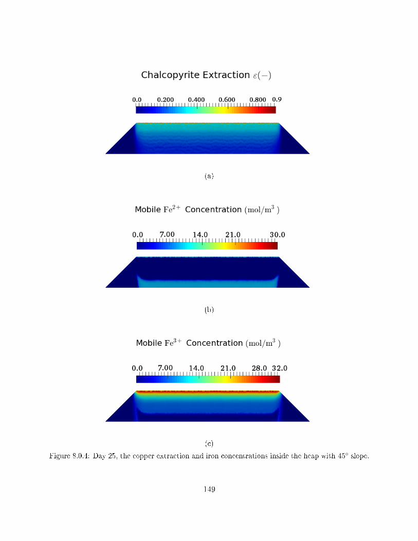
(a)

(b)

(c)

Figure 8.0.4: Day 25, the copper extraction and iron concentrations inside the heap with 45 slope.

149

(a)

(b)

(c)

(d)

Figure 8.0.5: Day 231, the copper and pyrite extractions and copper concentration inside the heap

with 45 slope.

150

(a)

(b)

(c)

(d)

Figure 8.0.6: Day 231, The mobile and immobile iron concentrations inside the heap with 45 slope.

151

(a)

(b)

(c)

(d)

Figure 8.0.7: Day 231, the rock, mobile liquid, immobile liquid temperature and total bacteria

population inside the heap with 45 slope.

152

Fe3+ ions are accumulated from the top to the bottom heap (Figures 8.0.6).

(a)

(b)

Figure 8.0.8: Day 231, The liquid pH inside the heap with 45 slope.

At the end of leaching (day 231), the chalcopyrite near the top of the heap are completely

extracted (Figure 8.0.5(a)), which may dier from the real system because some mineral

grains are likely to be completely inaccessible to the leaching solution. These grains would,

in reality, only be leached if additional pores or cracks were created. As is shown in Figures

8.0.5(a) and 8.0.5(b), the extraction of pyrite is lower than chalcopyrite, which is because

the lower dissolution rate of pyrite than chalcopyrite. Both the extraction of chalcopyrite

and pyrite are highest at the heap top and decrease from the top to the bottom, while the

extractions are extremely small near the two side walls due to the solution being almost

stagnant in those triangular zones. This is because the recants (Fe3+ and acid), bacteria

and heat are hardly transported into the triangular regions near the two walls for the whole

leaching period (Figures 8.0.6 to 8.0.8), and the heap temperature in those two regions is

153

always much colder than the middle rectangular region (Figures 8.0.7), which can result in

extremely slow reaction kinetics near the two heap walls. Most of the reactants are consumed

by the reactions in the middle rectangular region before they are dispersed to the two sides.

Figures 8.0.5(c) and 8.0.5(d) show that the copper concentration is highest in the two

triangular regions near the walls when the leaching ends. This reveals that copper ions

extracted in the earlier period , when the extraction rates were fast and the copper con-

centrations are high in the rectangular zone, are dispersed to the triangular regions by the

large concentration dierence, when the copper concentrations were signicantly lower in

the triangular zones. The two triangular regions act like `reservoirs' when the leaching rate

in the heap is fast, and the copper ions dispersed to these regions are trapped in both of the

dynamic and stagnant solution near the two walls, since the Darcy velocity is negligible in

those two regions Figure 8.0.2(b)). When the copper dissolution rates are decreased signi-

cantly, most of the copper ions extracted in the earlier period are transported to the leachate,

so the copper concentration in the middle rectangular region is decreased signicantly, and

the amount of mass left in the side triangular regions are higher. Then, the transport of the

copper ions in those regions is remarkably slow, since the rate at which the `reservoirs' release

the copper ions is mainly dependant on the slow dispersion by the concentration dierence

between the side triangular regions and the middle rectangular region. Thus, the existence

of the oblique slopes can cause a delay in the recovery of the extracted copper.

8.1 The Eect of The Heap Wall Slope

As is discussed above, due to the existence of the oblique walls, the rock near the walls

is hardly extracted, and some of the copper ions will be `stored' near the walls rather than

being delivered to the leachate. It is important to evaluate that the eect of the wall slope

on leaching. Two other simulations with walls slope of 30 and 60 are implemented, the

results when the leaching ends (on day 231) are shown in the following gures.

As is illustrated in Figures 8.1.1, the total liquid saturation near the two heap walls in-

creases with with increasing steepness of the slope. More dynamic liquid and less stagnant

154

liquid in the two triangular regions near the sides are present when the wall is steeper. It

can be observed that the heap with a 30 slope contains the most stagnant liquid as the

volume of the triangular regions are largest among the three dierent slope cases. While for

the heap with 60 slope, only the liquid near the two bottom tips are highly immobile since

the heap shape is closer to the natural spread angle of the liquid in this system.

(a) (b)

(c) (d)

(e) (f)

Figure 8.1.1: The liquid saturation inside the heap with 30 and 60 slope on Day 231.

The reactant concentrations for the three dierent slope cases distribute in the similar

prole from the top to the bottom when the leaching ended, for example Fe3+ concentra-

tions are highest near the heap top, but it is depleted quickly along the heap height (Figures

8.1.2(a) and 8.1.2(b)), and the pH is lowest when the fresh solution is supplied from the top

and the acidity is reduced vertically through the heap(Figures 8.1.2(c) and 8.1.2(d)), thus

155

(a) (b)

(c) (d)

(e) (f)

Figure 8.1.2: The dynamic Ferric concentrations, pH and liquid temperature inside the heap with

45 and 60 slope on Day 231.

indicating that changing the wall slope has little eect on the leach behaviour in the actively

owing central zone. However, as a result of the less stagnant and more dynamic liquid near

the wall of the steeper heap, more reactants can be transported to the two triangular zones

when increasing the wall slope. Especially when comparing the pH of 30 and 60 slope

models, it can be seen that the acid can be hardly distributed to the two sharp bottom tips

of the 30 model for the whole leaching period and the pH of the liquid in these corners

are near neutral. While in the model with 60 slope, the acids are transported to the two

corners, with the pH of the liquid in the two bottom tips being strongly acidic (around pH

of 4.5).

156

Since it is easier for the reactants access to the triangular regions of the heap with steeper

wall, the reactions in the regions around the two walls are promoted when increasing the

wall slope, as the results, more sulphide located in the triangular regions can be leached

(Figures 8.1.3(a) to 8.1.3(d)). Although the heap volume and total ore mass are kept the

same for the 30 , 45 and 60 slope models, the proportion of the volume in the triangu-

lar regions is more if the wall slope is shallower, more of the ore particles are within this

virtually unleached region and thus the overall extraction is lower. As a results, although

the vertical distributions through the middle rectangular region of either the chalcopyrite or

pyrite extraction are similar for the three slope cases, which is decreasing from the top to

(a) (b)

(c) (d)

(e) (f)

Figure 8.1.3: The chalcopyrite, pyrite extractions and dynamic copper concentrations inside the

heap with 45 and 60 slope on Day 231.

157

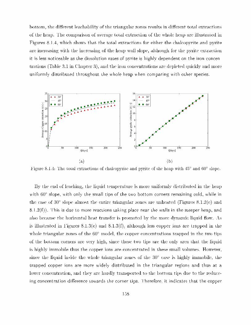
bottom, the dierent leachability of the triangular zones results in dierent total extractions

of the heap. The comparison of average total extraction of the whole heap are illustrated in

Figures 8.1.4, which shows that the total extractions for either the chalcopyrite and pyrite

are increasing with the increasing of the heap wall slope, although for the pyrite extraction

it is less noticeable as the dissolution rates of pyrite is highly dependent on the iron concen-

trations (Table 3.1 in Chapter 3), and the iron concentrations are depleted quickly and more

uniformly distributed throughout the whole heap when comparing with other species.

(a) (b)

Figure 8.1.4: The total extractions of chalcopyrite and pyrite of the heap with 45 and 60 slope.

By the end of leaching, the liquid temperature is more uniformly distributed in the heap

with 60 slope, with only the small tips of the two bottom corners remaining cold, while in

the case of 30 slope almost the entire triangular zones are unheated (Figures 8.1.2(e) and

8.1.2(f)). This is due to more reactions taking place near the walls in the steeper heap, and

also because the horizontal heat transfer is promoted by the more dynamic liquid ow. As

is illustrated in Figures 8.1.3(e) and 8.1.3(f), although less copper ions are trapped in the

whole triangular zones of the 60 model, the copper concentrations trapped in the two tips

of the bottom corners are very high, since these two tips are the only area that the liquid

is highly immobile thus the copper ions are concentrated in these small volumes. However,

since the liquid inside the whole triangular zones of the 30 case is highly immobile, the

trapped copper ions are more widely distributed in the triangular regions and thus at a

lower concentration, and they are hardly transported to the bottom tips due to the reduce-

ing concentration dierence towards the corner tips. Therefore, it indicates that the copper

158

ions are easier to transport to the leachate when increasing the wall slope since the volume

of the regions that can store the ions are reduced, and the liquid in most of the triangular

zones are more dynamic.

8.2 Conclusion

Three 2-D simulations of the trapezoid shape heap with three dierent wall slopes, which

are 30, 45 and 60, have been carried out. It was found that the oblique wall of the heap

can cause the liquid in triangular zones near the wall to be highly immobile, and thus the

vertical mass transport and heat transfer through these regions mainly depend on dispersion

rather than advection. This results in large `blank' zones near the wall to be unleached.

It was then found that by increasing the wall slope, that is making the heap shape closer

to a rectangle can promote the ow near the walls, and therefore more ore in the area of the

triangular zones can me extracted. It should be noted that in practice the slope of these walls

is limited by the stability or angle of repose of the packed particles of which the heap is com-

posed. It might therefore be worth investigating if the support measures that might required

to create steeper walls would be worth the economic benet of the additional copper recovery.

The investigations in this chapter showed that the mobile-immobile model works properly

to capture highly immobile zones near the triangular sides. The high immobile saturations

near the sides are found, which implicitly means that the axial dispersions near the sides

would deviate from those of a conventional ADE formulation signicantly. Therefore, the

investigations of the 2D heap scale modelling suggested that the mobile-immobile model

which can include the inhomogeneous distributions of immobile saturations and dispersions

would work better in predicting the leaching performance of a trapezoid heap.

159

Chapter 9

Conclusion and Future Work

The primary aim of this project was to develop a novel simulator and to use it to con-

duct computational modelling of mass transport and heat transfer phenomena in large scale

heap leaching. Fluidity, which is an open source simulator based on nite element and

control volume method was further developed to include the mobile-immobile model and

leaching chemical model for leaching simulation. Then mathematical formulations of our de-

veloped simulator is presented in Chapter 3, Darcy's law is applied to model the multiphase

ow inside the porous heap bed. To model the transport of the species inside heap, the

mobile-immobile model is employed instead of the conventional advection dispersion model

due to the presence of the stagnant liquid zones when the liquid is percolating through the

packed bed. Six main chemical reactions are considered for chalcopyrite leaching, which are

chalcopyrite dissolution, pyrite dissolution, oxidation of elemental sulphur, gangue mineral

dissolution, ferrous oxidation and jarosite precipitations. To include the bacterial eect, the

bio-leaching model which treats the bacterial activities as a catalytic eect on ferrous oxi-

dation is presented as an alternative to the traditional pure chemical ferrous oxidation. All

of the rate equations for these reactions are based on the previous literature.

The traditional methods in modelling mineral dissolutions of a porous ore are by the

shrinking core model (SCM), which normally classify the dissolution kinetics into three cat-

egories: chemical reaction control alone, diusion control alone and mixed control by both

reaction and diusion. However, by analysis of the base column leaching experiments in

Chapter 4, it was found that the the transition of the leaching mechanics from diusion

160

control to reaction control exists during leaching, and thus it might not be appropriate to

represent the dissolution kinetics by a xed SCM which is either reaction control or diusion

control. A newly developed semi-empirical model is then presented to be an alternative to

the traditional SCM. This model is more exible than the SCM approach of the diusion or

reaction control in ability to t with various dissolution kinetics proles, and dierent from

the mixed control type SCM approach, the new model does not need to over complicate the

mathematical formulation. The key assumption of this modelling approach is that the eect

of the bulk uid conditions (concentrations, temperatures, pH etc.) and the current state

of the particles (characterised by the current extent of extraction) on the leaching rate are

mathematically separable. It assumes that the non-linearities don't cause serious errors in

the separability. This separability assumption is validated in Chapter 5, with the maximum

error in the worst case being 5%, indicating that even if the leaching system is under mixed

control and highly non-linear, the error produced by making this assumption is still small.

The experimental conditions and data from experiments K1, K2 and K3 are also listed in

Chapter 4. The experiment K1 was used to calibrate the semi-empirical model in Chapter

5 and experiments K2 and K3 were used for validation of the numerical model. The exper-

imental errors in the extractions and solution concentrations were evaluated by analysing

the three repeat tests of K1. Then, to validate the numerical model, three 1D simulations

were implemented and compared with the laboratory results of K1, K2 and K3 separately

in Chapter 6. The results shows that the simulations can t the three experiments in a

satisfactory manner for both the extractions and solution concentrations, the simulations

and experiments were within the determined experimental uncertainty of one another. Also,

in Chapter 6, the solid-liquid heat transfer model was veried against the method of man-

ufactured solutions(MMS), and the mobile-immobile model is validated by the laboratory

tests. Separate convergence analyses were carried out for these two models, and he numer-

ical results converge to the analytical solutions or experimental results properly when the

temporal and spatial resolutions are rened. Thus, the new numerical models for leaching

are either validated or veried and can be used to implement various simulations.

The sensitivity analysis is necessary to evaluate the inuence of various factors on the

leaching system before an ecient heap can be designed. In Chapter 7, ve sets of 1D sim-

161

ulations were carried out to analyse the eects of bacterial activity, the form of the mass

transport model, solution temperature, Fe3+ concentrations and solution pH, and all of these

simulations are compared with a same base model. It is observed that the bacterial eect is

the most dominant eect among these 5 factors. The leaching rate can be improved signi-

cantly if the bacteria exist to play a catalyst role in ferrous oxidation. Due to the increased

production of Fe3+ by ferrous oxidation, the chalcopyrite extractions are increased by a large

amount, and the heap can be heated up signicantly by the large amount of heat released

by the increased ferrous oxidation rate and the net chalcopyrite dissolution rate. All of the

other 4 factors have minor eects on leaching if the bacterial eect is absent in the system,

and the nal copper extractions of the whole heap are little. Most of the Fe2+ in these 4

sets of models without bacteria just accumulated in the leachate without being converted to

Fe3+ , which indicates that the ferrous oxidation rate is a key factor in chalcopyrite leaching.

By comparing the leaching models with and without the eect of stagnant solutions, it

was found that the existence of stagnant zones can slightly slow the extraction rates, this is

caused by the temporal lag of the solution concentrations between the dynamic and stagnant

regions. The mass transfer between the mobile and immobile liquid can delay the solution

transport through the heap and thus lower the extraction rates. Except for the bacterial

eect, the increasing temperature can increase the leaching extractions most among the 4

factors, and raising the liquid temperature to as high as 50C can greatly improve the fer-

rous oxidation and thus promote the extraction rates. However, this improvement in Fe3+

generation is still tiny since the activation energy of ferrous oxidation is very high without

the bacterial catalyst, and the oxidation rates at a temperature of 50C still can not pro-

duce enough Fe3+ to signicantly improve copper extractions. The inuence of the Fe3+ and

solution pH are similar by doubling either the uid acidity or the Fe3+ concentrations of the

solutions applied from the top, the extractions can be improved to a similar extent.

Finally, the 2D simulations for the large scale leaching with a heap of trapezoid shape

are implemented in Chapter 8. To investigate the eect of the oblique walls on the leaching

performance, the leaching systems with three dierent wall slopes, 30, 45 and 60, are

evaluated. The applied liquid volumetric ow rate, the heap top area and the heap volume

are kept the same, and the applied simulation conditions and parameters are also kept the

162

same for these three models. It was then observed that the liquid inside the triangular re-

gions near the two oblique walls are highly immobile. This is because the liquid applied

from the heap top is mainly driven by gravity, while the horizontal spread of the liquid from

the middle rectangular region of the trapezoid heap to its triangle sides is mainly dependent

on the capillary actions of the porous bed, thus the saturation of the liquid near the two

walls is small. The reagents are mainly transported towards the walls by slower dispersion

rather than the faster advection. This results in negligible reactant concentrations within

the triangular regions so that large area near the walls remained unleached. Also, the tri-

angular region will act as a reservoir for some of the extracted copper ions. Those copper

ions are mainly dispersed to the immobile triangular zones via large concentration dierence

between the triangular zones and rectangular zone in the initial leaching period when the

dissolution rates are fast and copper concentrations inside the rectangular zone are large.

This can delay the gathering of the copper in the leachate since the releasing of copper ions

from those highly immobile regions is slow. By varying the walls slopes, it can be concluded

that the steeper the wall is, the more copper extraction can be achieved, that is the heap

performance is better if the trapezoid shape is closer to a rectangle and the volume of the

triangular zones are smaller.

9.1 Future Work

Most of the parameters and the rate equations used in the chemical models are from

literature which are not specically designed for leaching , so they might not be ideal for

application in leaching modelling since the conditions of the leaching system might dier sig-

nicantly from the conditions of the experiments used to obtain these parameters and rate

equations. Thus, it is desirable to calibrate the various reactions specically for the leaching

system. Also, the rate equations of jarosite precipitation, elemental sulphur oxidation, and

gangue mineral dissolution in our model are simply formulated to be linearly dependent on

the solution concentrations, which might be over simplied, thus more accurate formulations

are needed to optimize the numerical model.

One of the concerns in using the new semi-empirical model is that each calibration of

163

the model is only valid for a certain type of the ore with certain size. The curve of the

semi-empirical model represents the apparent kinetics of the dissolutions of the ores in the

base experiments used for calibrations, however, the apparent kinetics might vary largely if

the size and the type of the ore are changed. Since the distributions of mineral grain and

grade inside an ore fragment is dependent on the type of the ore, and the size and the shape

will also inuence the grain distributions and the leachablety of the ore, thus, it might be

erroneous to use only one calibrated semi-empirical curve to predict the real world leaching

which contains dierent ore fragment sizes throughout the heap. Therefore, it is desirable

to calibrate the semi-empirical model with dierent ore sizes, and even dierent ore types

if the investigations of the leaching performance with dierent ores are required. Then, for

each specic type of ore, a complete semi-empirical model with a catalogue of semi-empirical

curves for dierent ore sizes can be used in the real leaching system with the considerations

of the particle size distributions inside the heap.

Finally, when the chemical models are newly calibrated and also the semi-empirical model

is completed by calibration with dierent ore sizes, the optimisation of heap leaching system,

perfectly in 3D modelling, can be carried out. The extent to which each factor will inuence

heap leaching will be analysed in detail rather than the simple sensitivity analysis in this

thesis, and under the consideration of the industry issues, a practical optimised combination

of the parameters which can improve the leaching eciency could be determined. Ideally this

would be coupled within an economic model so that the costs and benets of each change

can be quantitatively assumed.

164

References

[1] Acero, P., Cama, J., and Ayora, C. Kinetics of chalcopyrite dissolution at ph 3.

European Journal of Mineralogy 19, 2 (2007), 173182.

[2] Adebayo, A., Ipinmoroti, K., and Ajayi, O. Dissolution kinetics of chalcopyrite

with hydrogen peroxide in sulphuric acid medium. Chemical and biochemical engineer-

ing quarterly 17, 3 (2003), 213218.

[3] Ahonen, L., and Tuovinen, O. H. Bacterial leaching of complex sulde ore samples

in bench-scale column reactors. Hydrometallurgy 37, 1 (1995), 121.

[4] Al-Dahhan, M. H., and Dudukovi¢, M. P. Catalyst wetting eciency in trickle-

bed reactors at high pressure. Chemical Engineering Science 50, 15 (1995), 23772389.

[5] AMCG. Fluidity Manual. Department of Earth Science and Engineering, South Kens-

ington Campus, Imperial College London, London, 2012.

[6] Andersson, C., Führer, C., and Åkesson, J. Assimulo: A unied framework for

ode solvers. Mathematics and Computers in Simulation 116 (2015), 2643.

[7] Antonijevi¢, M., and Bogdanovi¢, G. Investigation of the leaching of chalcopy-

ritic ore in acidic solutions. Hydrometallurgy 73, 3 (2004), 245256.

[8] Aydogan, S., Ucar, G., and Canbazoglu, M. Dissolution kinetics of chalcopyrite

in acidic potassium dichromate solution. Hydrometallurgy 81, 1 (2006), 4551.

[9] Bartlett, R. W. Simulation of ore heap leaching using deterministic models. Hy-

drometallurgy 29, 1 (1992), 231260.

[10] Bartlett, R. W. Solution mining: Leaching and uid recovery of materials. Psy-

chology Press, 1998.

165

[11] Bartlett, R. W. Solution mining: Leaching and uid recovery of materials. Psy-

chology Press, 1998.

[12] Baur, J., Gibbs, H., and Wadsworth, M. Initial-stage sulric acid leaching

kinetics of chalcopyrite using radiochemical techniques. united states bureau of mines.

Report of Investigations USBM RI 7823 (1974).

[13] Bear, J. Dynamics of uids in porous media. Dover Civil and Mechanical Engineering

Series. DOVER PUBN Incorporated, 1972.

[14] Beckstead, L., Munoz, P., Sepulveda, J., Herbst, J., Miller, J., Olson, F.,

and Wadsworth, M. Acid ferric sulphate leaching of attritor-ground chalcopynte

concentrates. In Intern. Symp. On Copper Extraction and Rening, Las Vegas, Nevada

(1976), vol. 11, pp. 611633.

[15] Bennett, C., McBride, D., Cross, M., and Gebhardt, J. A comprehensive

model for copper sulphide heap leaching: Part 1 basic formulation and validation

through column test simulation. Hydrometallurgy 127 (2012), 150161.

[16] Bennett, C., McBride, D., Cross, M., Gebhardt, J., and Taylor, D. Sim-

ulation technology to support base metal ore heap leaching. Mineral Processing and

Extractive Metallurgy 115, 1 (2006), 4148.

[17] Boon, M., and Heijnen, J. Mechanisms and rate limiting steps in bioleaching of

sphalerite, chalcopyrite and pyrite with thiobacillus ferrooxidans. Biohydrometallurgi-

cal Technologies 1 (1993), 1993217.

[18] Bouffard, S. C. Application of the heapsim model to the heap bioleaching of the

pueblo viejo ore deposit. Hydrometallurgy 93, 3 (2008), 116123.

[19] Bouffard, S. C., and Dixon, D. G. Investigative study into the hydrodynamics

of heap leaching processes. Metallurgical and Materials Transactions B 32, 5 (2001),

763776.

[20] Bouffard, S. C., and Dixon, D. G. Modeling pyrite bioleaching in isothermal test

columns with the heapsim model. Hydrometallurgy 95, 3 (2009), 215226.

166

[21] Brandl, H., Rehm, H., and Reed, G. Biotechnology, special processes. Wiley-

VCH, Weinheim 10 (2001), 191.

[22] Braun, R. L., Lewis, A. E., and Wadsworth, M. E. In-place leaching of primary

sulde ores: Laboratory leaching data and kinetics model. Metallurgical Transactions

5, 8 (1974), 17171726.

[23] Brittan, M. Variable activation energy model for leaching kinetics. International

Journal of Mineral Processing 2, 4 (1975), 321 331.

[24] Brooks, R. H., and Corey, A. T. Hydraulic properties of porous media. Hydrology

Papers, Colorado State University, March (1964).

[25] Buckley, A. N., and Woods, R. An x-ray photoelectron spectroscopic study of the

oxidation of chalcopyrite. Australian Journal of Chemistry 37, 12 (1984), 24032413.

[26] Cemi£, L., and Kleppa, O. High temperature calorimetry of sulde systems. Physics

and chemistry of minerals 16, 2 (1988), 172179.

[27] Chae, D., and Wadsworth, M. In situ recovery of minerals. Engineering Founda-

tion, New York, NY (1989), 121.

[28] Córdoba, E. Nuevas evidencias sobre los mecanismos de lixiviación química y biológ-

ica de la calcopirita. PhD thesis, PhD Thesis. Universidad Complutense de Madrid,

2005.

[29] Córdoba, E., Muñoz, J., Blázquez, M., González, F., and Ballester, A.

Leaching of chalcopyrite with ferric ion. part i: General aspects. Hydrometallurgy 93,

3 (2008), 8187.

[30] Córdoba, E., Muñoz, J., Blázquez, M., González, F., and Ballester, A.

Leaching of chalcopyrite with ferric ion. part II: Eect of redox potential. Hydromet-

allurgy 93, 3 (2008), 8896.

[31] Corey, A. T. The interrelation between gas and oil relative permeabilities. Producers

monthly 19, 1 (1954), 3841.

167

[32] Cross, M., Bennett, C., Croft, T., McBride, D., and Gebhardt, J. Com-

putational modeling of reactive multi-phase ows in porous media: Applications to

metals extraction and environmental recovery processes. Minerals Engineering 19, 10

(2006), 10981108.

[33] de Andrade Lima, L. A mathematical model for isothermal heap and column

leaching. Brazilian Journal of Chemical Engineering 21, 3 (2004), 435447.

[34] de Andrade Lima, L. Liquid axial dispersion and holdup in column leaching. Min-

erals engineering 19, 1 (2006), 3747.

[35] de Andrade Lima, L. Liquid axial dispersion and holdup in column leaching. Min-

erals Engineering 19, 1 (2006), 3747.

[36] Decker, D., and Tyler, S. Evaluation of ow and solute transport parameters for

heap leach recovery materials. Journal of Environmental Quality 28, 2 (1999), 543555.

cited By 19.

[37] Deveci, H. Eect of particle size and shape of solids on the viability of acidophilic

bacteria during mixing in stirred tank reactors. Hydrometallurgy 71, 3 (2004), 385396.

[38] Dixon, D., and Hendrix, J. A general model for leaching of one or more solid

reactants from porous ore particles. Metallurgical Transactions B 24, 1 (1993), 157

169.

[39] Dixon, D., and Petersen, J. Comprehensive modelling study of chalcocite column

and heap bioleaching. In Copper (2003), vol. 6, pp. 493516.

[40] Dixon, D. G. Analysis of heat conservation during copper sulphide heap leaching.

Hydrometallurgy 58, 1 (2000), 2741.

[41] Dixon, D. G., and Hendrix, J. L. A mathematical model for heap leaching of one

or more solid reactants from porous ore pellets. Metallurgical Transactions B 24, 6

(1993), 10871102.

[42] Dreisinger, D., and Abed, N. A fundamental study of the reductive leaching of

chalcopyrite using metallic iron part I: kinetic analysis. Hydrometallurgy 66, 1 (2002),

3757.

168

[43] Dullien, F. A. Porous media: uid transport and pore structure. Academic press,

2012.

[44] DUTIZAC, J., MAC, D., and Ingraham, T. The kinetics of dissolution of synthetic

chalcopyrite in aqueous acidic ferric sulfate solutions. TRANS MET SOC AIME 245,

5 (1969), 955959.

[45] Dutrizac, J. The dissolution of chalcopyrite in ferric sulfate and ferric chloride media.

Metallurgical and Materials Transactions B 12, 2 (1981), 371378.

[46] Dutrizac, J. Elemental sulphur formation during the ferric sulphate leaching of

chalcopyrite. Canadian Metallurgical Quarterly 28, 4 (1989), 337344.

[47] Dwivedy, K., and Mathur, A. Bioleachingâour experience. Hydrometallurgy

38, 1 (1995), 99109.

[48] Ferrier, R. J., Cai, L., Lin, Q., Gorman, G. J., and Neethling, S. J. Models

for apparent reaction kinetics in heap leaching: A new semi-empirical approach and

its comparison to shrinking core and other particle-scale models. Hydrometallurgy 166

(2016), 2233.

[49] Flury, M., and Gimmi, T. F. 6.2 solute diusion. Methods of Soil Analysis: Part

4 Physical Methods, methodsofsoilan4 (2002), 13231351.

[50] Fogler, H., and Brown, L. Distributions of residence times for chemical reactors.

Elements of Chemical Reaction Engineering (1992), 708758.

[51] Fu, K.-b., Lin, H., Mo, X.-l., Wang, H., Wen, H.-w., and Wen, Z.-l. Compar-

ative study on the passivation layers of copper sulphide minerals during bioleaching.

International Journal of Minerals, Metallurgy, and Materials 19, 10 (2012), 886892.

[52] Gao, H., Sohn, H., and Wadsworth, M. A mathematical model for the solution

mining of primary copper ore: Part i. leaching by oxygen-saturated solution containing

no gas bubbles. Metallurgical Transactions B 14, 4 (1983), 541551.

[53] Gao, H., Sohn, H., and Wadsworth, M. A mathematical model for the solution

mining of primary copper ore: Part ii. leaching by solution containing oxygen bubbles.

Metallurgical Transactions B 14, 4 (1983), 553558.

169

[54] Garcia, X., Akanji, L. T., Blunt, M. J., Matthai, S. K., and Latham, J. P.

Numerical study of the eects of particle shape and polydispersity on permeability.

Phys. Rev. E 80 (Aug 2009), 021304.

[55] Gbor, P. K., and Jia, C. Q. Critical evaluation of coupling particle size distribution

with the shrinking core model. Chemical Engineering Science 59, 10 (2004), 19791987.

[56] Gbor, P. K., and Jia, C. Q. Critical evaluation of coupling particle size distribution

with the shrinking core model. Chemical Engineering Science 59, 10 (2004), 19791987.

[57] Ghorbani, Y., Becker, M., Mainza, A., Franzidis, J.-P., and Petersen, J.

Large particle eects in chemical/biochemical heap leach processes-A review. Minerals

Engineering 24, 11 (2011), 1172 1184. Special Issue : Bio and Hydrometallurgy.

[58] Hackl, R., Dreisinger, D., Peters, E., and King, J. Passivation of chalcopyrite

during oxidative leaching in sulfate media. Hydrometallurgy 39, 1 (1995), 2548.

[59] Harmer, S. L., Thomas, J. E., Fornasiero, D., and Gerson, A. R. The evolu-

tion of surface layers formed during chalcopyrite leaching. Geochimica et Cosmochimica

Acta 70, 17 (2006), 43924402.

[60] Harneit, K., Göksel, A., Kock, D., Klock, J.-H., Gehrke, T., and Sand,

W. Adhesion to metal sulde surfaces by cells of acidithiobacillus ferrooxidans,

acidithiobacillus thiooxidans and leptospirillum ferrooxidans. Hydrometallurgy 83, 1

(2006), 245254.

[61] Herbst, J. A. Rate processes in multiparticle metallurgical systems. In Rate processes

of extractive metallurgy. Springer, 1979, pp. 53112.

[62] Herbst, J. A. Rate processes in multiparticle metallurgical systems. In Rate processes

of extractive metallurgy. Springer, 1979, pp. 53112.

[63] Herrera, M. N., Wiertz, J. V., Ruiz, P., Neuburg, H. J., and Badilla-

Ohlbaum, R. A phenomenological model of the bioleaching of complex sulde ores.

Hydrometallurgy 22, 1 (1989), 193 206.

[64] Hirato, T., Majima, H., and Awakura, Y. The leaching of chalcopyrite with

ferric sulfate. Metallurgical Transactions B 18, 3 (1987), 489496.

170

[65] Hiroyoshi, N., Kuroiwa, S., Miki, H., Tsunekawa, M., and Hirajima, T. Syn-

ergistic eect of cupric and ferrous ions on active-passive behavior in anodic dissolution

of chalcopyrite in sulfuric acid solutions. Hydrometallurgy 74, 1 (2004), 103116.

[66] Hiroyoshi, N., Miki, H., Hirajima, T., and Tsunekawa, M. Enhancement of

chalcopyrite leaching by ferrous ions in acidic ferric sulfate solutions. Hydrometallurgy

60, 3 (2001), 185197.

[67] Hiroyoshi, N., Tsunekawa, M., Okamoto, H., Nakayama, R., and Kuroiwa,

S. Improved chalcopyrite leaching through optimization of redox potential. Canadian

Metallurgical Quarterly (2013).

[68] Howard, D., and Crundwell, F. A kinetic study of the leaching of chalcopyrite

with sulfolobus metallicus. Process Metallurgy 9 (1999), 209217.

[69] Hsu, P., and Murr, L. A simple kinetic model for sulfuric acid leaching of copper

from chrysocolla. Metallurgical Transactions B 6, 3 (1975), 435440.

[70] Ilankoon, I., Cole, K., and Neethling, S. Measuring hydrodynamic dispersion

coecients in unsaturated packed beds: Comparison of PEPT with conventional tracer

tests. Chemical Engineering Science 89, 0 (2013), 152 157.

[71] Iliuta, I., Thyrion, F., and Muntean, O. Axial dispersion of liquid in gas-liquid

cocurrent downow and upow xed-bed reactors with porous particles. Chemical

Engineering Research and Design 76, 1 (1998), 6472.

[72] Jones, D., and Peters, E. Leaching of chalcopyrite with ferric sulfate and ferric

chloride. Extractive Metallurgy of Copper. 2 (1976).

[73] Jones, E., Oliphant, T., Peterson, P., et al. SciPy: Open source scientic

tools for Python, 2001. [Online; accessed 2016-09-16].

[74] Kametani, H., and Aoki, A. Eect of suspension potential on the oxidation rate

of copper concentrate in a sulfuric acid solution. Metallurgical Transactions B 16, 4

(1985), 695705.

[75] Kaplun, K., Li, J., Kawashima, N., and Gerson, A. Cu and fe chalcopyrite

leach activation energies and the eect of added fe 3+. Geochimica et Cosmochimica

Acta 75, 20 (2011), 58655878.

171

[76] Kimball, B. E., Rimstidt, J. D., and Brantley, S. L. Chalcopyrite dissolution

rate laws. Applied Geochemistry 25, 7 (2010), 972983.

[77] Kirjavainen, V., and Heiskanen, K. Some factors that aect beneciation of

sulphide nickelcopper ores. Minerals Engineering 20, 7 (2007), 629633.

[78] Klauber, C. A critical review of the surface chemistry of acidic ferric sulphate

dissolution of chalcopyrite with regards to hindered dissolution. International Journal

of Mineral Processing 86, 1 (2008), 117.

[79] Klauber, C., Parker, A., van Bronswijk, W., and Watling, H. Sulphur

speciation of leached chalcopyrite surfaces as determined by x-ray photoelectron spec-

troscopy. International Journal of Mineral Processing 62, 1 (2001), 6594.

[80] Koleini, S. J., Aghazadeh, V., and Sandström, Å. Acidic sulphate leaching

of chalcopyrite concentrates in presence of pyrite. Minerals Engineering 24, 5 (2011),

381386.

[81] Kougianos, A., van Bronswijk, W., Klauber, C., et al. Characterisation of

metal polysulphides. Chemeca 2000: Opportunities and Challenges for the Resource

and Processing Industries (2000), 80.

[82] Kuwahara, F., Shirota, M., and Nakayama, A. A numerical study of interfacial

convective heat transfer coecient in two-energy equation model for convection in

porous media. International journal of heat and mass transfer 44, 6 (2001), 1153

1159.

[83] Lakatos, B., and Blickle, T. Eect of particle size distribution on liquidâsolid

reaction kinetics in solutions. Acta Chimica Hungarica 127, 2 (1990), 395405.

[84] Lara, R. H., Vazquez-Arenas, J., Ramos-Sanchez, G., Galvan, M., and

Lartundo-Rojas, L. Experimental and theoretical analysis accounting for dier-

ences of pyrite and chalcopyrite oxidative behaviors for prospective environmental and

bioleaching applications. The Journal of Physical Chemistry C 119, 32 (2015), 18364

18379.

172

[85] Leahy, M., Davidson, M., and Schwarz, M. A model for heap bioleaching of

chalcocite with heat balance: mesophiles and moderate thermophiles. Hydrometallurgy

85, 1 (2007), 2441.

[86] Leahy, M. J. Temperature and air ow eects in the modelling of bacteria in heap

bioleaching of chalcocite. PhD thesis, 2006.

[87] Leahy, M. J., and Schwarz, M. P. Modelling jarosite precipitation in isothermal

chalcopyrite bioleaching columns. Hydrometallurgy 98, 1 (2009), 181191.

[88] LeBlanc, S., and Fogler, H. Population balance modeling of the dissolution of

polydisperse solids: rate limiting regimes. AIChE journal 33, 1 (1987), 5463.

[89] Levenspiel, O. Chemical reaction engineering (3rd edition). TY: GEN.

[90] Li, Y., Kawashima, N., Li, J., Chandra, A., and Gerson, A. A review of the

structure, and fundamental mechanisms and kinetics of the leaching of chalcopyrite.

Advances in colloid and interface science 197 (2013), 132.

[91] Liddell, K. C. Shrinking core models in hydrometallurgy: what students are not

being told about the pseudo-steady approximation. Hydrometallurgy 79, 1 (2005),

6268.

[92] Lin, Q. Use of X-ray Computed Microtomography to Measure the Leaching Behaviour

of Metal Sulphide Ores. Published PhD thesis. Imperial College London, 2015.

[93] Lin, Q., Neethling, S., Courtois, L., Dobson, K., and Lee, P. Multi-scale

quantication of leaching performance using x-ray tomography. Hydrometallurgy 164

(2016), 265277.

[94] Linge, H. Reactivity comparison of australian chalcopyrite concentrates in acidied

ferric solution. Hydrometallurgy 2, 3 (1977), 219233.

[95] Liu, H.-c., Xia, J.-l., and Nie, Z.-y. Relatedness of cu and fe speciation to chal-

copyrite bioleaching by acidithiobacillus ferrooxidans. Hydrometallurgy 156 (2015),

4046.

[96] Lowson, R. T. Aqueous oxidation of pyrite by molecular oxygen. Chemical Reviews

82, 5 (1982), 461497.

173

[97] Madsen, B., GROVES, R., and WADSWORTH, M. Application of a mixed

kinetics model to the leaching of low grade copper sulde ores. Trans. Soc. Min. Eng.

AIME 258, 1 (1975), 6974.

[98] Madsen, B., Wadsworth, M., and of Mines, U. S. B. A mixed kinetics dump

leaching model for ores containing a variety of copper sulde minerals. Report of

investigations. U.S. Dept. of the Interior, Bureau of Mines, 1981.

[99] Malik, A., Dastidar, M. G., and Roychoudhury, P. Factors limiting bacte-

rial iron oxidation in biodesulphurization system. International Journal of Mineral

Processing 73, 1 (2004), 1321.

[100] Masterton, W., and Hurley, C. Chemistry: principles and reactions. Cengage

Learning, 2015.

[101] Mateos, F. B., Pérez, I. P., and Mora, F. C. The passivation of chalcopyrite

subjected to ferric sulfate leaching and its reactivation with metal suldes. Hydromet-

allurgy 19, 2 (1987), 159167.

[102] Mazuelos, A., Palencia, I., Romero, R., Rodriguez, G., and Carranza, F.

Ferric iron production in packed bed bioreactors: inuence of ph, temperature, particle

size, bacterial support material and type of air distributor. Minerals Engineering 14,

5 (2001), 507514.

[103] McBride, D., Croft, T., Cross, M., Bennett, C., and Gebhardt, J. Op-

timization of a cfdheap leach model and sensitivity analysis of process operation.

Minerals Engineering 63 (2014), 5764.

[104] Meruane, G., and Vargas, T. Bacterial oxidation of ferrous iron by acidithiobacil-

lus ferrooxidans in the ph range 2.57.0. Hydrometallurgy 71, 1 (2003), 149158.

[105] Mikhlin, Y. L., Tomashevich, Y. V., Asanov, I. P., Okotrub, A. V., Varnek,

V. A., and Vyalikh, D. V. Spectroscopic and electrochemical characterization of

the surface layers of chalcopyrite (cufes 2) reacted in acidic solutions. Applied Surface

Science 225, 1 (2004), 395409.

[106] Miller, G. Ore geotechnical eects on copper heap leach kinetics. Young, CA, et

al.(Ed.), Hydrometallurgy (2003), 329342.

174

[107] Mostaghimi, P., Tollit, B. S., Neethling, S. J., Gorman, G. J., and Pain,

C. C. A control volume nite element method for adaptive mesh simulation of ow in

heap leaching. Journal of Engineering Mathematics 87, 1 (2014), 111121.

[108] Munoz, P., Miller, J. D., and Wadsworth, M. E. Reaction mechanism for the

acid ferric sulfate leaching of chalcopyrite. Metallurgical Transactions B 10, 2 (1979),

149158.

[109] Neuburg, H. J., Castillo, J. A., Herrera, M. N., Wiertz, J. V., Vargas,

T., and Badilla-Ohlbaum, R. A model for the bacterial leaching of copper sulde

ores in pilot-scale columns. International Journal of Mineral Processing 31, 3 (1991),

247 264.

[110] Nicol, M., Miki, H., and Velásquez-Yévenes, L. The dissolution of chalcopyrite

in chloride solutions: Part 3. mechanisms. Hydrometallurgy 103, 1 (2010), 8695.

[111] Ogbonna, N., Petersen, J., and Dixon, D. G. Heapsimunravelling the mathe-

matics of heap bioleaching. In Computational analysis in hydrometallurgy, 35th annual

hydrometallurgy meeting. CIM-MetSoc, Montreal (2005), pp. 225240.

[112] Olubambi, P., Ndlovu, S., Potgieter, J., and Borode, J. Eects of ore min-

eralogy on the microbial leaching of low grade complex sulphide ores. Hydrometallurgy

86, 1 (2007), 96104.

[113] Padilla, G. A., Cisternas, L. A., and Cueto, J. Y. On the optimization of

heap leaching. Minerals Engineering 21, 9 (2008), 673678.

[114] Padilla, R., Pavez, P., and Ruiz, M. Kinetics of copper dissolution from suldized

chalcopyrite at high pressures in h 2 so 4o 2. Hydrometallurgy 91, 1 (2008), 113120.

[115] Papanastassiou, D., and Bitsianes, G. Modelling of heterogeneous gas-solid

reactions. Metallurgical Transactions 4, 2 (1973), 477486.

[116] Park, J., and Levenspiel, O. The crackling core model for the reaction of solid

particles. Chemical Engineering Science 30, 10 (1975), 12071214.

[117] Parker, A., Klauber, C., Kougianos, A., Watling, H., and Van Bronswijk,

W. An x-ray photoelectron spectroscopy study of the mechanism of oxidative dissolu-

tion of chalcopyrite. Hydrometallurgy 71, 1 (2003), 265276.

175

[118] Parker, A., Paul, R., and Power, G. Electrochemistry of the oxidative leaching

of copper from chalcopyrite. Journal of Electroanalytical Chemistry and Interfacial

Electrochemistry 118 (1981), 305316.

[119] Patankar, S. Numerical heat transfer and uid ow. CRC press, 1980.

[120] Paul, B. C., Sohn, H., and Mccarter, M. K. Model for ferric sulfate leaching of

copper ores containing a variety of sulde minerals: Part i. modeling uniform size ore

fragments. Metallurgical Transactions B 23, 5 (1992), 537548.

[121] Peiró, J., and Sherwin, S. Finite dierence, nite element and nite volume

methods for partial dierential equations. In Handbook of materials modeling. Springer,

2005, pp. 24152446.

[122] Petersen, J. Modelling of bioleach processes: Connection between science and en-

gineering. Hydrometallurgy 104, 3â4 (2010), 404 409. <ce:title>18th Interna-

tional Biohydrometallurgy Symposium, IBS2009, Bariloche-Argentina, 13-17 Septem-

ber 2009</ce:title>.

[123] Petersen, J., and Dixon, D. Systematic modelling of heap leach processes for opti-

misation and design. In EPD Congress 2002 and Fundamentals of Advanced Materials

for Energy Conversion as Held at the 2002 TMS Annual Meeting (2002), pp. 757771.

[124] Petersen, J., and Dixon, D. Modelling zinc heap bioleaching. Hydrometallurgy

85, 2â4 (2007), 127 143.

[125] Petersen, J., and Dixon, D. G. Modeling and optimization of heap bioleach

processes. In Biomining. Springer, 2007, pp. 153176.

[126] Pradhan, N., Nathsarma, K., Rao, K. S., Sukla, L., and Mishra, B. Heap

bioleaching of chalcopyrite: a review. Minerals Engineering 21, 5 (2008), 355365.

[127] Prasad, S., and Pandey, B. Alternative processes for treatment of chalcopyrite-a

review. Minerals Engineering 11, 8 (1998), 763781.

[128] Putnis, A. An Introduction to Mineral Sciences. Cambridge University Press, 1992.

[129] Roache, P. J. Code verication by the method of manufactured solutions. Journal

of Fluids Engineering 124, 1 (2002), 410.

176

[130] Rossi, G. Biohydrometallurgy. McGraw-Hill, 1990.

[131] Sanchez-Chacon, A., and Lapidus, G. Model for heap leaching of gold ores by

cyanidation. Hydrometallurgy 44, 1 (1997), 120.

[132] Sandström, Å., and Petersson, S. Bioleaching of a complex sulphide ore with

moderate thermophilic and extreme thermophilic microorganisms. Hydrometallurgy

46, 1 (1997), 181190.

[133] Sandström, Å., Shchukarev, A., and Paul, J. Xps characterisation of chalcopy-

rite chemically and bio-leached at high and low redox potential. Minerals Engineering

18, 5 (2005), 505515.

[134] Scanlon, B. R., Nicot, J. P., and Massmann, J. W. Soil gas movement in

unsaturated systems. Handbook of soil science (2000), A277A319.

[135] Senanayake, G. A review of chloride assisted copper sulde leaching by oxygenated

sulfuric acid and mechanistic considerations. Hydrometallurgy 98, 1 (2009), 2132.

[136] Sidborn, M., Casas, J., Martnez, J., and Moreno, L. Two-dimensional dy-

namic model of a copper sulphide ore bed. Hydrometallurgy 71, 1 (2003), 6774.

[137] Smith, J. M. Chemical engineering kinetics. McGraw-Hill, 1981.

[138] Sohn, H., and Szekely, J. A structural model for gas-solid reactions with a moving

boundary-III: A general dimensionless representation of the irreversible reaction be-

tween a porous solid and a reactant gas. Chemical Engineering Science 27, 4 (1972),

763778.

[139] Soki¢, M. D., Markovi¢, B., and ivkovi¢, D. Kinetics of chalcopyrite leaching

by sodium nitrate in sulphuric acid. Hydrometallurgy 95, 3 (2009), 273279.

[140] Strömberg, B., and Banwart, S. A. Experimental study of acidity-consuming

processes in mining waste rock: some inuences of mineralogy and particle size. Applied

Geochemistry 14, 1 (1999), 116.

[141] Szekely, J. Gas-solid reactions. Elsevier, 2012.

177

[142] Szekely, J., and Themelis, N. J. Rate phenomena in process metallurgy. John

wiley & Sons Inc., New York, (1971).

[143] Third, K., Cord-Ruwisch, R., and Watling, H. The role of iron-oxidizing

bacteria in stimulation or inhibition of chalcopyrite bioleaching. Hydrometallurgy 57,

3 (2000), 225233.

[144] Tromans, D. Oxygen solubility modeling in inorganic solutions: concentration, tem-

perature and pressure eects. Hydrometallurgy 50, 3 (1998), 279296.

[145] Vafai, K., and Sozen, M. Analysis of energy and momentum transport for uid

ow through a porous bed. Journal of Heat Transfer 112, 3 (1990), 690699.

[146] Van Swaaij, W., Charpentier, J., and Villermaux, J. Residence time distri-

bution in the liquid phase of trickle ow in packed columns. Chemical Engineering

Science 24, 7 (1969), 10831095.

[147] Veglio, F., Trifoni, M., Pagnanelli, F., and Toro, L. Shrinking core model

with variable activation energy: a kinetic model of manganiferous ore leaching with

sulphuric acid and lactose. Hydrometallurgy 60, 2 (2001), 167179.

[148] Villanueva, I., Heresi, N., Henriquez, P., and Vega, P. Tracer techniques

in the study of ow patterns in leaching tanks. International Journal of Radiation

Applications and Instrumentation. Part 41, 10-11 (1990), 11591163. cited By 2.

[149] Wadsworth, M. Rate processes in hydrometallurgy. In 2nd Tutorial Symposium on

Extractive Met., University of Utah (1972).

[150] Wagman, D. D., Evans, W. H., Parker, V. B., Schumm, R. H., and Halow,

I. The nbs tables of chemical thermodynamic properties. selected values for inorganic

and c1 and c2 organic substances in si units. Tech. rep., DTIC Document, 1982.

[151] Wakao, N., and Kagei, S. Heat and mass transfer in packed beds, vol. 1. Taylor &

Francis, 1982.

[152] Watling, H. The bioleaching of sulphide minerals with emphasis on copper sulphides-

A review. Hydrometallurgy 84, 1 (2006), 81108.

178

[153] Wen, C. Noncatalytic heterogeneous solid-uid reaction models. Industrial & Engi-

neering Chemistry 60, 9 (1968), 3454.

[154] Williamson, M. A., and Rimstidt, J. D. The kinetics and electrochemical rate-

determining step of aqueous pyrite oxidation. Geochimica et Cosmochimica Acta 58,

24 (1994), 54435454.

[155] Yagi, S., and Kunii, D. 5th symposium (international) on combustion. Reinhold,

New York (1955), 231.

[156] Yahya, A., and Johnson, D. Bioleaching of pyrite at low ph and low redox poten-

tials by novel mesophilic gram-positive bacteria. Hydrometallurgy 63, 2 (2002), 181

188.

[157] Yang, Y., Liu, W., and Chen, M. A copper and iron k-edge xanes study on

chalcopyrite leached by mesophiles and moderate thermophiles. Minerals Engineering

48 (2013), 3135.

[158] Yang, Y., Liu, W., and Chen, M. Xanes and xrd study of the eect of ferrous and

ferric ions on chalcopyrite bioleaching at 30Â° c and 48Â° c. Minerals Engineering 70

(2015), 99108.

[159] Yu, R.-L., Tan, J.-X., Peng, Y., Jing, S., Ouyang, X.-J., and Dai, Y.-J. Eps-

contact-leaching mechanism of chalcopyrite concentrates by a. ferrooxidans. Transac-

tions of Nonferrous Metals Society of China 18, 6 (2008), 14271432.

179

Appendix A

Experimental Data

The calculated extraction of chalcopyrite and pyrite from experiment K1 are illustrated

in Figure A.0.1:

(a) Average extraction of copper in the column (b) Average extraction of pyrite in the column

Figure A.0.1: The calculated extraction of chalcopyrite and pyrite of column experiment K1 from

experimental data.

The data from the repeated experiments for K1 from Lin(2015) [92] are listed in Figures

A.0.2:

180

(a) Average extraction of copper in

the column

(b) Copper concentration in the

leachate form the column bottom

(c) The redox potential of the

leachate form the bottom of the col-

umn

(d) The concentration of iron in the

leachate form the bottom of the col-

umn

(e) pH of the leachate from the bot-

tom of the column

Figure A.0.2: The experimental data of the repeated experiments of K1

181

cfd modelling of chalcopyrite heap leaching · the main contribution of this project is that a new...

Documents