1

Verification and Validation Database of American Society of Civil Engineers 2008

Copyright © American Society of Civil Engineers

VERIFICATION AND VALIDATION OF URBAN

ATMOSPHERIC FLOW MODELS

PART II: COMPARISON OF VARIOUS TURBULENCE

MODELS Andy Chan

1 & Hervé Morvan

2

1 School of Chemical and Environmental Engineering,

University of Nottingham Malaysia Campus,

Jalan Broga, 43500 Semenyih, Selangor Darul Ehsan, Malaysia.

2 Department of Mechanical Engineering, University of Nottingham,

University Park, Nottingham NG7 2RD, United Kingdom.

0. ABSTRACT

This second paper of the series compares the performance of different turbulent models

applied on different standard benchmark test on urban atmospheric flow problems

described in Part I. The k- model, the Reynolds-stress model and large-eddy simulation

are compared against available experimental and computational data. The details of each

turbulence model are described and their limitations and working conditions elaborated

and an assessment is made.

1. INTRODUCTION

One of the objectives of scientific inquiry rests on to develop a logical quantitative theory

that can give accurate prediction to a natural phenomenon. The study of urban

atmospheric flow problems is no exception. The problem, however, is that our

experience has told us there are no prospects of a simple, single, embracing theory that

can govern turbulent air flow (Pope 2002). In fact the study of the turbulence remains

one of the mysteries of modern physics. In spite of the existence of a robust theory, there

is no single simple methodology of solution to the full Navier-Stokes equations, due to its

high nonlinearity and variations of boundary conditions. No single physical problems in

physics invite the appearance of such a rich diversity of models to solve the equation

while no one understands for certain which one remains a good explanation.

Until recently, the main tool to understand turbulent fluid motions has been the statistical

models. With the advancement of computational resources, various newer models based

on the Navier-Stokes equations have been derived and solutions from them have been

made possible. Others, which have been developed earlier but could not be put in

practice, like the Direct Numerical Simulations (DNS) have been realised bit by bit.

2

All these different models, obviously give different results, even for the same problems

and to a certain extent, proper analytical understanding has been procastinated. The fact

is that different models are given birth from a vastly different objective, perspective and

philosophy and it is inevitable that they differ from each other in results and predictions.

Different models also agree with experimental data at different extent. A model that

gives good agreement in one case can be very poor in a different situation. It is with this

objective that this paper is prepared, to illustrate the philosophies behind each model and

to describe and explain the performance of each model under the profiled benchmark

tests.

2. CHOICE OF TURBULENCE MODELS

It might be useful to give a brief account of the various turbulence models that are

frequently employed in practical engineering calculations of turbulent airflows. A more

in-depth study of various turbulence models can be found in most standard textbooks of

fluid mechanics (Pope 2002) and various review papers (Rodi 1997).

Before elaborating the technical details of various models, it is also important to outline

the various factors over the choice of model. After all there are so many models

available and it is thus important to know the criteria of selection over a wide range of

attributes.

As outlined in Pope (2002), a number of assessment criteria for model selection are

available which could include:

i) level of modeling,

ii) computational resources available,

iii) applicability and usability,

iv) accuracy…

It is important to note that this list is definitely subjective and non-exhaustive and any

extra criteria that are deemed necessary should be included.

2.1 Level of Modelling

In Direct Numerical Simulations (DNS), there is absolutely no ‘artificial’ modelling

involved. The velocity components are solved directly from the Navier-Stokes equations

at the Kolmogorov’s scales. The velocities are also obtained at instantaneous level and

statistics can be immediately extracted. At the other end of the spectrum, the mixing-

length model specifies various flow parameters: some physical, some even natural. This

model is deemed incomplete. Moreover, when using mixing length model, the velocity is

calculated to the mean values only. Velocity fluctuations or turbulence statistics

informations cannot be obtained directly.

2.2 Computational Resources

One important attribute to decide which turbulence model to use is the availability of

computational resources. Speaking based on the same computer hardware requirement,

3

obviously the computational resources required increases with the required precision.

Yet some models like DNS requires many more times resources than conventional

models using the Reynolds-averaged Navier-Stokes equations (RANS) approach. In

some approach like DNS, the resources required is a function of the Reynolds number of

the flow, while simpler models only depend on the precision expected.

2.3 Applicability And Usability

Each model is designed and derived for a different application and definitely so models

are not applicable a particular flow phenomenon. In fact there is no single model that is

applicable to all flows, at least from an accuracy point of view. Mixing-length models

are in general confined to application of lower Reynolds numbers only because of their

derivation from the laminar principles. The various empirical constants of say, k-

models are tweaked from one application to another in order to match the experimental

data to varying degree of accuracy.

Some models, like DNS or Large-eddy simulations (LES) are applicable to a wider range

of applications due to their lower artificiality. On the other hand, they are usually not

commercially usable as their huge computational cost prohibits extensive engineering

applications, at least in present.

2.4 Accuracy

Accuracy is of course of fundamental importance. There are however a large number of

issues which could incur errors into the system. One very important subject is the

prescription of boundary condition in turbulent flows. As mentioned in Part I of the

paper, there are a lot of difficulties in the computational study of urban atmospheric flows

and all the mentioned issues incur inaccuracies into the solution to varying degree.

Different models incur different sort of inaccuracies according to their own

characteristics and it is important to know the model’s deficiencies before application.

3. TURBULENCE MODELS

3.1 Reynolds-Averaged Navier-Stokes Equations

Without going through trivialities which available in most standard texts, the Reynolds-

averaged Navier-Stokes (RANS) equations are given by

ij

ji

ii

x

P

x

uuU

Dt

DU

1''2

, (1)

following usual notations, where the capital letters refer to the mean flow parameters and

the minuscules + prime refer to the fluctuation parts. The key to solve the RANS

equations lies in closing the equations through modelling of the Reynolds-stress term

j

ji

x

uu

'', which is itself undeterminable. Modelling of different kinds have been

4

developed to handle this particular term and relate this to various mean properties. We

shall only focus on the various models that are commonly used in engineering.

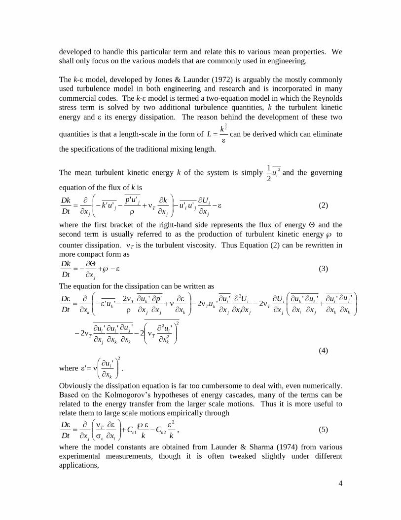
The k- model, developed by Jones & Launder (1972) is arguably the mostly commonly

used turbulence model in both engineering and research and is incorporated in many

commercial codes. The k- model is termed a two-equation model in which the Reynolds

stress term is solved by two additional turbulence quantities, k the turbulent kinetic

energy and its energy dissipation. The reason behind the development of these two

quantities is that a length-scale in the form of

23

kL can be derived which can eliminate

the specifications of the traditional mixing length.

The mean turbulent kinetic energy k of the system is simply 2

2

1iu and the governing

equation of the flux of k is

j

iji

j

T

j

j

j x

Uuu

x

kupuk

xDt

Dk''

'''' (2)

where the first bracket of the right-hand side represents the flux of energy and the

second term is usually referred to as the production of turbulent kinetic energy to

counter dissipation. T is the turbulent viscosity. Thus Equation (2) can be rewritten in

more compact form as

jxDt

Dk (3)

The equation for the dissipation can be written as

2

2

2

2

'2

'''2

''''2

''2

''2''

k

iT

k

j

k

i

j

iT

k

j

k

i

j

k

i

k

j

iT

ji

i

j

ikT

kjj

kTk

k

x

u

x

u

x

u

x

u

x

u

x

u

x

u

x

u

x

U

xx

U

x

uu

xx

p

x

uu

xDt

D

(4)

where

2

''

k

i

x

u.

Obviously the dissipation equation is far too cumbersome to deal with, even numerically.

Based on the Kolmogorov’s hypotheses of energy cascades, many of the terms can be

related to the energy transfer from the larger scale motions. Thus it is more useful to

relate them to large scale motions empirically through

kC

kC

xxDt

D

i

T

j

2

21

, (5)

where the model constants are obtained from Launder & Sharma (1974) from various

experimental measurements, though it is often tweaked slightly under different

applications,

5

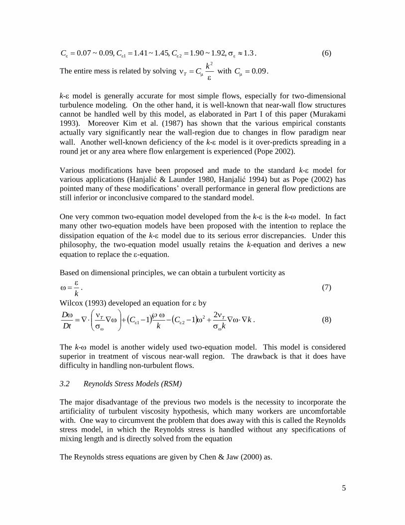
3.1,92.1~90.1,45.1~41.1,09.0~07.0 21 CCC . (6)

The entire mess is related by solving

2kCT

with 09.0C .

k- model is generally accurate for most simple flows, especially for two-dimensional

turbulence modeling. On the other hand, it is well-known that near-wall flow structures

cannot be handled well by this model, as elaborated in Part I of this paper (Murakami

1993). Moreover Kim et al. (1987) has shown that the various empirical constants

actually vary significantly near the wall-region due to changes in flow paradigm near

wall. Another well-known deficiency of the k- model is it over-predicts spreading in a

round jet or any area where flow enlargement is experienced (Pope 2002).

Various modifications have been proposed and made to the standard k- model for

various applications (Hanjalić & Launder 1980, Hanjalić 1994) but as Pope (2002) has

pointed many of these modifications’ overall performance in general flow predictions are

still inferior or inconclusive compared to the standard model.

One very common two-equation model developed from the k- is the k- model. In fact

many other two-equation models have been proposed with the intention to replace the

dissipation equation of the k- model due to its serious error discrepancies. Under this

philosophy, the two-equation model usually retains the k-equation and derives a new

equation to replace the -equation.

Based on dimensional principles, we can obtain a turbulent vorticity as

k

. (7)

Wilcox (1993) developed an equation for by

kk

Ck

CDt

D TT

211 2

21 . (8)

The k- model is another widely used two-equation model. This model is considered

superior in treatment of viscous near-wall region. The drawback is that it does have

difficulty in handling non-turbulent flows.

3.2 Reynolds Stress Models (RSM)

The major disadvantage of the previous two models is the necessity to incorporate the

artificiality of turbulent viscosity hypothesis, which many workers are uncomfortable

with. One way to circumvent the problem that does away with this is called the Reynolds

stress model, in which the Reynolds stress is handled without any specifications of

mixing length and is directly solved from the equation

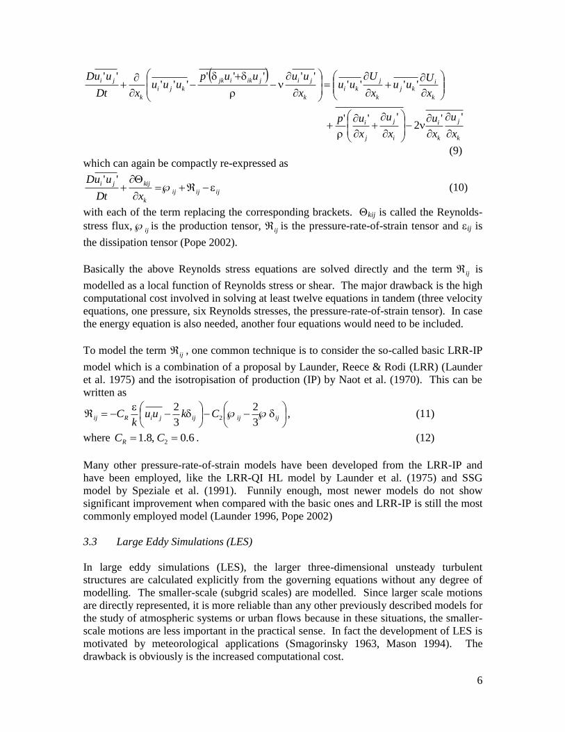
The Reynolds stress equations are given by Chen & Jaw (2000) as.

6

k

j

k

i

i

j

j

i

k

ikj

k

j

ki

k

jijikijk

kji

k

ji

x

u

x

u

x

u

x

up

x

Uuu

x

Uuu

x

uuuupuuu

xDt

uuD

''2

'''

'''''''''

'''''

(9)

which can again be compactly re-expressed as

ijijij

k

kijji

xDt

uuD

'' (10)

with each of the term replacing the corresponding brackets. kij is called the Reynolds-

stress flux, ij is the production tensor, ij is the pressure-rate-of-strain tensor and ij is

the dissipation tensor (Pope 2002).

Basically the above Reynolds stress equations are solved directly and the term ij is

modelled as a local function of Reynolds stress or shear. The major drawback is the high

computational cost involved in solving at least twelve equations in tandem (three velocity

equations, one pressure, six Reynolds stresses, the pressure-rate-of-strain tensor). In case

the energy equation is also needed, another four equations would need to be included.

To model the term ij , one common technique is to consider the so-called basic LRR-IP

model which is a combination of a proposal by Launder, Reece & Rodi (LRR) (Launder

et al. 1975) and the isotropisation of production (IP) by Naot et al. (1970). This can be

written as

ijijijjiRij Ckuu

kC

3

2

3

22 , (11)

where 6.0,8.1 2 CCR . (12)

Many other pressure-rate-of-strain models have been developed from the LRR-IP and

have been employed, like the LRR-QI HL model by Launder et al. (1975) and SSG

model by Speziale et al. (1991). Funnily enough, most newer models do not show

significant improvement when compared with the basic ones and LRR-IP is still the most

commonly employed model (Launder 1996, Pope 2002)

3.3 Large Eddy Simulations (LES)

In large eddy simulations (LES), the larger three-dimensional unsteady turbulent

structures are calculated explicitly from the governing equations without any degree of

modelling. The smaller-scale (subgrid scales) are modelled. Since larger scale motions

are directly represented, it is more reliable than any other previously described models for

the study of atmospheric systems or urban flows because in these situations, the smaller-

scale motions are less important in the practical sense. In fact the development of LES is

motivated by meteorological applications (Smagorinsky 1963, Mason 1994). The

drawback is obviously is the increased computational cost.

7

The equations of motions of LES are derived by applying the filter to the Navier-Stokes

equations. The filter of LES is essentially the grid resolution such that the details of the

velocity field can be adequately resolved within the domain concerned. We shall just

illustrate the basic equation and the detailed technicalities of LES are given by Pope

(2002). Using the bar as representation of filtered variables, the equations of motion of

LES are

2

21

0

i

j

ji

jij

i

i

x

U

x

p

x

UU

t

U

x

U

(13)

The momentum equation can also be written as

u

ttD

D

xx

U

x

p

tD

UD

i

r

ij

i

j

j

j:

12

2

(14)

where ij is the residual stress tensor.

The closure of the nonlinear convective term in LES is usually handled by the

Smagorinsky model, which is analogous to the eddy-viscosity model in Reynolds stress,

ijr

r

ij S 2 and ijSSr SSSCSl 2:22 (15)

where r is the residual eddy viscosity, ls is the Smagorinsky lengthscale analogous to the

mixing length and Cs is the Smagorinsky’s coefficient proportional to the filter width .

The original Smagorinsky’s model is that the appropriate value of the Smagorinsky’s

constant varies in different flow regime and assigning it a constant value brings

inaccuracies within the domain. Recently Germano et al. (1991) proposed the dynamic

LES in which Smagorinsky’s value at each point in space is calculated based on the flow

domain and surrounding flow parameters.

Compared with RANS or RSM models, LES has the advantage of describing without

modelling the instantaneous large-scale turbulent flow structures, meaning that the

solutions are exact solutions of the Navier-Stokes equations. Therefore LES has been

receiving large attention in the aerodynamics and environmental sector lately. The

problem of LES, however is obviously its larger computational cost. Pope (2002) also

reported that LES are likely to be grid-dependent as it depends on a priori knowledge of

the flow structure, especially the subgrid scale motions. LES is also restrictively three-

dimensional and unsteady and unless three-dimensional unsteady solutions are truly

sought, sometimes the computational cost can be lavish.

In terms of accuracy, LES is reasonably accurate for most free shear flows (Piomelli

1993, Vreman et al. 1997) but since LES has only recently picked up its momentum,

fingers should still be kept crossed.

4. BENCHMARK RESULTS

8

4.1 Lid Driven Cavity Test

Ghia et al. (1982) have presented numerical solutions for the lid-driven cavity flow for

various Reynolds number, and further validated by Ertürk et al. (2002). As mentioned in

Part I of the paper, the results of Ghia et al. (1982) are largely regarded as the standard

data for comparison purposes. Botella & Peyret (1998) used a Chebyshev collocation

method for the solution of the lid-driven cavity flow and obtained highly accurate

spectral solutions for the cavity flow for Reynolds numbers Re 9,000. They stated that

their numerical solutions exhibit a periodic behavior beyond this Re. Both of which can

validated with experiments at lower Reynolds numbers.

As mentioned in Part I of the paper, it is often useful to look and analyse the positions of

all the vortices developed, including the centre main vortex and the few corner vortices.

Figure 1 shows the location and approximate features of these vortex centres.

Figure 1: Flow structure within a lid-driven cavity (Ertürk et al. 2002)

Figure 2: Flow structure within lid-driven cavity under different Reynolds numbers

a) Re = 100, b) Re = 1000, and c) Re = 10000 (Ghia et al. 1982)

Figure 2 shows the computational results of Ghia et al. (1982) under different Reynolds

numbers, while Figure 3 shows the computational validation results of Ertürk et al.

9

(2002). Comparisons are made with the location of the various vortices and the velocity

profile at the mid-section of the cavity as in Figure 3. The use of streamfunctions and

vorticity in this test case also favours comparison using streamline plots and vorticity

plots and vorticity plots have also been made.

Figure 3: Flow structures of lid-driven cavity flow at Re = 10000 and the horizontal

velocities at different Re by Ertürk et al. (2002)

It must be emphasised here that there had been many computational evidences that the

lid-driven cavity test cannot be extended for larger Reynolds number (Shankar &

Deshpande 2000). Many of the data show that instability and unsteadiness ensue beyond

Re > 15000 and disallows proper comparisons. The case is similar to vortex shedding of

flow past cylinder in large Reynolds number flows where comparison at any time-instant

is difficult.

4.2 Backward Facing Step Test

Driver & Seegmiller (1985) performed wind-tunnel experiments on the backward facing

step test and the data have been frequently used for comparison purposes. The setup is a

step-height to tunnel-exit-height ratio of 1:10 which would reduce free-stream pressure

changes at the expansion step. The tunnel is 12 times wider than the tunnel height to

reduce three-dimensional effect. The data are also available at NPARC Alliance website

(http://www.grc.nasa.gov/WWW/wind/valid/backstep/backstep.html).

To compare the results, the wind profile at each axial position and the length of the

separation zone is looked at. In general it is expected that the k- model would predict

the reattachment to occur too far upstream (Thangam 1992, Yoder & Georgiadis 1999).

Figure 4 shows the experimental data of the velocity profiles.

10

Figure 4: Velocity profiles of the backward facing step test at various axial positions

(Yoder & Georgiadis 1999)

4.3 T-Junction Test

11

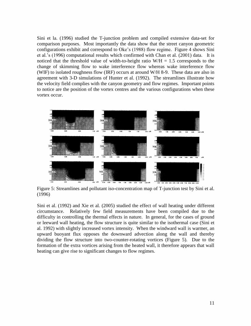
Sini et la. (1996) studied the T-junction problem and compiled extensive data-set for

comparison purposes. Most importantly the data show that the street canyon geometric

configurations exhibit and correspond to Oke’s (1988) flow regime. Figure 4 shows Sini

et al.’s (1996) computational results which confirmed with Chan et al. (2001) data. It is

noticed that the threshold value of width-to-height ratio W/H = 1.5 corresponds to the

change of skimming flow to wake interference flow whereas wake interference flow

(WIF) to isolated roughness flow (IRF) occurs at around W/H 8-9. These data are also in

agreement with 3-D simulations of Hunter et al. (1992). The streamlines illustrate how

the velocity field complies with the canyon geometry and flow regimes. Important points

to notice are the position of the vortex centres and the various configurations when these

vortex occur.

Figure 5: Streamlines and pollutant iso-concentration map of T-junction test by Sini et al.

(1996)

Sini et al. (1992) and Xie et al. (2005) studied the effect of wall heating under different

circumstance. Relatively few field measurements have been compiled due to the

difficulty in controlling the thermal effects in nature. In general, for the cases of ground

or leeward wall heating, the flow structure is quite similar to the isothermal case (Sini et

al. 1992) with slightly increased vortex intensity. When the windward wall is warmer, an

upward buoyant flux opposes the downward advection along the wall and thereby

dividing the flow structure into two-counter-rotating vortices (Figure 5). Due to the

formation of the extra vortices arising from the heated wall, it therefore appears that wall

heating can give rise to significant changes to flow regimes.

12

Figure 6: Streamlines and pollutant iso-concentration map of T-junction test for different

cases of heating by Sini et al. (1996)

4.4 Indoor Ventilation Test

The simplicity of geometry of the indoor ventilation allows extensive measurements to be

taken. Data are compared for the velocity at different axial direction and the location of

the recirculating vortex. It is worthwhile to notice that the indoor ventilation test

resembles the backward step physically and many of the features are expected to be

similar. Nielsen (1990) and Nielsen et al. (1978) had performed extensive wind-tunnel

and numerical experiments and had compiled useful data for comparisons as illustrated in

Figure 7 and 8.

13

Figure 6: Velocity profiles of the indoor ventilation test (Nielsen 1990)

For the thermal case, temperature and the penetration depths are the two extra variables

to be compared with as in Figure 7 and 8. The temperature, velocity and the penetration

depths are compared for various Archimedes number, which is essentially the Grashof

number in convection. Data for comparisons are also available from Lemaire (1993).

14

Figure 7: Temperature distribution in the indoor ventilation test for various Archimedes

number (Nielsen 1990)

Figure 8: Penetration depth for the indoor ventilation test (Nielsen 1990)

4.5 Personal Exposure Test

Brohus (1997) documented the velocity profile and pollutant concentration profile for the

personal exposure test (Figure 9 and 10)

15

Figure 9: Velocity distribution for personal exposure test (Brohus 1997)

Figure 10: Contaminant concentration profile for personal exposure test (Brohus 1997)

4.6 Flow Round Cube

A seminal discussion on flow past a cube (or square cylinder) is available in Rodi (1997).

In general the phenomena of vortex shedding should be reproduced by all models. As

available in the literatures, the shedding produced by LES is not as regular as produced

by RSM or RANS models. Most models should be able to produce good agreement with

experimental data near the cylinder. On the other hand as expected different models

would produce different results in the outer domain. The standard k- model over-

predicts the separation zone length whereas the RSM models produce too short a region

(Murakami 1993, Murakami & Mochida 1995).

There have been data aplenty regarding the various flow parameters near a cube as listed

in the references mentioned. Centreline velocity comparisons have been mostly used to

study the flow structures and compare the features of different model. Figure 11 shows

the centreline mean velocities for flow past cube calculated using different model

(Murakami 1993) and compared with experimental data. Comparisons are focused along

velocities, pressure and vorticity distribution and their corresponding vortex-shedding

phenomena.

16

Figure 11: Centreline velocity of flow past cube (Murakami 1993)

4.7 Flow Past a Two-Dimensional Hill

Yu et al. (2003) studied the flow past a two-dimensional topographical changes in the

form of a smooth hill and a steep cliff. The well-known shortcomings of the k- model

in over-predicting the development of turbulent kinetic energy near the sharp edges are

well exhibited. Aside from comparing with the various parameters, separation points and

recirculation regions are also looked at. Figure 12 shows the wind profile of flow pas a

2D hill for comparison purposes.

Figure 12: Wind profile along a 2D hill (Yu et al. 2003)

5. REFERENCES

17

Botella, O. & Peyret, R. 1998, Benchmark spectral results on the lid-driven cavity flow, Computers and

Fluids vol. 27, pp. 421-433

Chan, A.T., So, E.S.P. & Samad, S.C. 2001, Strategic guidelines for street canyon geometry to achieve

sustainable air quality, Atmospheric Environment vol. 25 no. 32, pp. 5681-5691.

Chen, J.Y. & Jaw, S.Q. 2000, Introduction to turbulence modeling, Prentice Hall

Driver, D.M. and Seegmiller, H.L. 1985, Features of a reattaching turbulent shear layer in divergent

channel flow, AIAA Journal vol. 23, no. 2, pp. 163-171

Ertürk, E., Corke, T.C. & Ğökçöl, Ç. 2005, Numerical solutions of 2-D steady incompressible driven cavity

flow at high Reynolds numbers, International Journal for Numerical Methods in Fluids vol. 48, pp. 747-774

Germano, M., Piomelli, U., Moin, P. & Cabot, W.H. 1991, A dynamic subgrid-scale eddy viscosity model,

Physics of Fluids A vol. 3, pp. 1760-1765

Ghia, U., Ghia, K.N. & Shin, G.T. 1982, High-Re solutions for incompressible flow using the Navier-

Stokes equations and the multigrid method, Journal of Computational Physics vol. 48, pp. 387-411

Hanjalić, K. 1994, Advanced turbulence closure models: a view of current status and future prospects,

International Journal of Heat and Fluid Flow vol. 15, pp. 178-203

Hanjalić, K. & Launder, B.E. 1980, Sensitizing the dissipation equation to irrotational strains, ASME

Journal of Fluids Engineering vol. 102, pp. 34-40

Hunter, L.J., Johnson, G.T. & Watson, I.D. 1992, An investigation of three-dimensional characteristics of

flow regimes within the urban canyon, Atmospheric Environment vol. 26B, pp. 425-432

Jones, W.P. & Launder, B.E. 1972, The prediction of laminarization with a two-equation model of

turbulence, International Journal of Heat and Mass Transfer vol. 15, pp. 301-314

Kim, J., Moin, P. & Moser, R. 1987, Turbulence statistics in fully developed channel flow at low Reynolds

number, Journal of Fluid Mechanics vol. 177, pp. 133-166

Launder, B.E. 1996, An introduction to single-point closure methodology, In Simulations and Modeling of

Turbulent Flows, pp. 243-310, Oxford University Press

Launder, B.E., Reece, G.J. & Rodi, W. 1975, Progress in the development of a Reynolds-stress turbulence

closure, Journal of Fluid Mechanics vol. 68, pp. 537-566

Launder, B.E. & Sharma. B.I. 1974, Application of the energy-dissipation model of turbulence to the

calculation of flow near a spinning disc, Letters of Heat and Mass Transfer vol. 1, pp 131-138

Lemaire, A.D. 1993, Room air and contaminant flow, evaluation of computational methods summary

report, International Energy Agency: Energy Conservation in Buildings and Community Systems

Programme Annex 20

Mason, P.J. 1994, Large eddy simulation: a critical review of the technique, Quarterly Journal of Royal

Meteorological Society vol. 120, pp. 1-26

Murakami, S. 1993, Comparison of various turbulence models applied to a bluff body, Journal of Wind

Engineering and Industrial Aerodynamics vol. 46/47, pp. 21-36

Murakami, S. & Mochida, A. 1995, On turbulent vortex shedding flow past 2D square cylinder predicted

by CFD, Journal of Wind Engineering and Industrial Aerodynamics vol. 54/55, pp. 191-211

18

Naot, D., Shavit, A. & Wolfshtein, M. 1970, Interactions between components of the turbulent velocity

correlation tensor due to pressure fluctuations, Israel Journal of Technology vol. 8, pp. 259-269

Nielsen, P.V. 1990, Specification of a two-dimensional test case, International Energy Agency, Energy

Conservation in Buildings and Community Systems Annex 20: Air Flow Pattern within Buildings

Nielsen, P.V., Restivo, A. & Whitelaw, J.H. 1978, The velocity characteristics of ventilated rooms, Journal

of Fluids Engineering vol. 100, pp. 291-298

Oke, T.R. 1988, Street design and urban canopy layer climate, Energy and Building vol. 11, pp. 103-113

Piomelli, U. 1993, High Reynolds number calculations using the dynamic subgrid-scale stress model,

Physics of Fluids A vol. 5, pp. 1484-1490

Pope, S.B. 2002, Turbulent Flows, Cambridge University Press

Rodi, W. 1997, Comparison of LES and RANS calculations of the flow around bluff bodies, Journal of

Wind Engineering and Industrial Aerodynamics vol. 69-71, pp 55-75

Shankar, P.N. & Deshpande, M.D. 2000, Fluid mechanics in the driven cavity, Annual Review of Fluid

Mechanics vol. 33, pp. 93-136

Smagorinsky, J. 1963, General circulation experiments with the primitive equations: I. The basic equations,

Monthly Weather Review vol. 91, pp. 99-164

Speziale, C.G., Sarkar, S. & Gatski, T.B. 1991, Modelling the pressure-strain correlation of turbulence: an

invariant dynamical systems approach, Journal of Fluid Mechanics vol. 227, pp. 245-272

Thangam, S. 1992, Turbulent flow past a backward-facing step: a critical evaluation of two-equation model,

AIAA Journal vol. 30, pp. 1314-1320

Vreman, B., Geurts, B. & Kuerten, H. 1997, Large eddy simulation of the turbulent mixing layer, Journal

of Fluid Mechanics vol. 339, pp. 357-390

Wilcox, D.C. 1993, Turbulence modeling for CFD, DCW Industries

Xie, X., Huang, Z., Wang, J. & Xie, Z. 2005, The impact of solar radiation and street layout on pollutant

dispersion in street canyon, Building and Environment vol. 40 no. 2, pp. 201-212

Yoder, D.A. & Georgiadis, N.J. 1999, Implementation and validation of the Chien k-epsilon turbulence

model in the WIND Navier-Stokes Code, AIAA Paper 99-0745

Yu, F.L., Mochida, A., Murakami, S., Yoshino, H. & Shirasawa, T. 2003, Numerical simulation of flow

over topographic features by revised k- model, Journal of Wind Engineering and Industrial Aerodynamics

vol. 9, pp. 231-245