cfd calculation of stability and control derivatives for ...cfd calculation of stability and control...

CFD Calculation of Stability and Control Derivatives

For Ram-Air Parachutes

Mehdi Ghoreyshi1∗, Keith Bergeron2†

Andrew J. Lofthouse1‡, Russell M. Cummings1§

1 High Performance Computing Research Center, U.S. Air Force Academy

USAF Academy, Colorado 808402 US Army Natick Research, Development, and Engineering Center

Natick, MA 01760

Generation of aerodynamic models for ram-air parachutes is currently the subject ofactive research. These parachutes resemble a rectangular wing of low aspect ratio. Theaerodynamic characteristics of these unswept wings can be very different from those pre-dicted by lifting-line theory due to openings in the leading edge for the admission of ramair. This research specifically investigates the aerodynamics of ram-air parachutes withopen and closed round inlets. All wings are assumed to be rigid and have an aspect ratioof two. Aerodynamic predictions are made with flow solvers of Cobalt and Kestrel andare compared with available wind-tunnel experimental data. Simulations and measure-ments are carried out at a Mach number of 0.25 and Reynolds number of 1.4 million. Theaerodynamic changes are predicted due to pulling the left trailing edge down. Aerody-namic stability derivatives are calculated from simulations of forced periodic motions indirections of pitch, yaw, and roll. The effects of motion reduced frequency are studied aswell. Two different estimation methods are used, namely linear regression method and amethod based on points of maximum and minimum angular velocity. The experimentaldata of wings considered here match the computational predictions quite well. For thewings with a left-side bending, the lift and drag will increase, the pitch moment at thequarter chord point will decreases and wing will produce a positive roll and a negative yawmoment. The open wings stall earlier than the closed wings, have higher pressure-dragvalues, and the pitch moment slope becomes more negative. The calculated derivatives aresimilar for both methods and show only a small change with reduced frequencies less than0.1. The results show that damping derivatives of closed wings remain fairly constant upto ten degrees angle of attack. However, the open wings show a very sensitive behaviorin damping derivatives with respect to angles of attack. Finally, the models are evaluatedfor the closed and open wings undergoing a chirp motion. The results of the comparisonshow that the aerodynamic models of the closed wing match time-marching full CFD cal-culations well, but some discrepancies can be seen in the open wing plots. The lift valuesfrom model and full CFD do not match everywhere and there is a time lag between pitchmoment predictions and time-marching solution, suggesting substantial unsteady effects onthe numerical simulations of open wings during the motion.

∗Senior Aerospace Engineer, AIAA Senior Member†Senior Research Aerospace Engineer, AIAA Senior Member‡Director, AIAA Senior Member§Professor of Aeronautics, AIAA Associate Fellow“The views expressed in this paper are those of the author and do not reflect the official policy or position of the United

States Air Force, Department of Defense, or the U.S. Government.” Distribution A. Approved for Public Release. Distributionunlimited.

1 of 21

American Institute of Aeronautics and Astronautics

Nomenclature

A motion amplitude, rada speed of sound, m/sb wing span, mCD drag coefficient, D/q∞SCL lift coefficient, L/q∞SCLα lift coefficient curve slope, 1/radCMx roll moment coefficient, Mx/q∞SbCMxβ derivative of roll moment coefficient with respect to sideslip angle, 1/radCMy , Cm pitch moment coefficient, My/q∞ScCMyα pitch moment coefficient curve slope, 1/radCMz yaw moment coefficient, Mx/q∞SbCMzβ derivative of yaw moment coefficient with respect to sideslip angle, 1/radCp pressure coefficientCY side-force coefficient, Y/q∞SCY β derivative of side-force coefficient with respect to sideslip angle, 1/radc mean aerodynamic chord, mD drag force, Nf frequency, Hzk reduced frequency, ωc/2VL lift force, NMx roll moment, N-mMy pitch moment, N-mMz yaw moment, N-mM Mach number, V/aPDF pitch damping force, 1/rad, CLq + CLα̇

PDM pitch damping moment, 1/rad, CMyq + CMyα̇

p̄, q̄, r̄ roll, pitch, and yaw rates,rad/sp normalized roll rate, p̄b/2Vq normalized pitch rate, q̄c/2VRDF roll damping force, 1/rad, CY p

RDM1 roll damping of roll moment, 1/rad, CMxp

RDM2 roll damping of yaw moment, 1/rad, CMzp

r normalized yaw rate, r̄b/2Vq∞ dynamic pressure, Pa, ρV 2/2Re Reynolds number, ρV c/µS Planform area, m3

V freestream velocity, m/sx, y, z aircraft position coordinatesYDF yaw damping force, 1/rad, CY r + CY β̇

YDM1 yaw damping of roll moment, 1/rad, CMxr + CMxβ̇

YDM2 yaw damping of yaw moment, 1/rad, CMzr + CMzβ̇

Greek

α angle of attack, radα̇ time-rate of change of angle of attack, rad/sβ sideslip angle, radα̇ time-rate of change of side-slip angle, rad/sδ trailing edge deflection angle, radϕ roll (bank) angle, radρ air density, kg/m3

µ air viscosity, kg/(m.s)ω angular velocity, rad/s

2 of 21


I. Introduction

The U.S. Army Natick Soldier Center manages and coordinates the DoD program to develop precisionguided airdrop systems known as the Joint Precision Airdrop System (JPADS). JPADS provides the abilityto deliver to multiple drop zones as quickly as possible, reduces the ground resupply risks and costs, and alsoallows the delivery aircraft to avoid hazardous objective areas.1 JPADS has shown very promising results,but there is still an increasing demand for enhancing the reliability and landing precision of these airdropsystems. This is a very challenging task because these systems are expected to operate from altitudes up to35,000 feet and to have a release point up to 40 km from the drop zone.2,3

Current precision aerial delivery systems use a large ram-air parachute (parafoil) integrated with a GlobalPositioning System (GPS) equipment, a navigation and a control system.4 These airdrop designs couldachieve a landing accuracy of 100 meters or even less depending on the control unit performance.4 Thecontrol performance will also depend on the accuracy of aerodynamic models for various drop conditions.

The aerodynamic models used in the design of parafoils are typically empirical or semi-empirical meth-ods generated from wind tunnel experiments and drop tests.5 For novel parachute designs, there are noexperimental data available to design control laws. Parachute designers might use the low-speed wing aero-dynamic to estimate the lift and drag coefficients.6,7 However, these estimates can yield very different resultsfrom those measured in tests due to openings in the leading edge of parachutes for the admission of ramair. As noted in the previous studies,8,9, 10,11 for a given shape, the open wings have different aerodynamiccharacteristic than the closed wings.

There is a new focus on generation of aerodynamic models of ram-air parachutes using ComputationalFluid Dynamics(CFD) simulations. This study is a continuation of previous collaborations between U.S.Air Force Academy (USAFA) and the U.S. Army Natick Soldier Center (NSC) on the application of CFDfor design and simulation of new ram-air parachutes. A previous publication by the authors has attemptedto generate CFD-based aerodynamic models for flight simulation of ram-air parachutes.11 The parachutegeometries were modeled as rigid rectangular wings with an aspect ratio of two and zero anhedral angle. Alinear regression model was used to estimate the stability derivatives from forced periodic motions. Thesederivatives were only estimated at eight degrees angle of attack. The results showed that the models matchfull CFD data which were used to create the models.

This study extends these previous results by calculation of stability derivative at different angles of attackand investigating the effects of motion frequency on stability derivatives. CFD predictions are validatedwith additional experimental data. Two different estimation methods are used in this work, namely linearregression method and a method based on points of maximum and minimum angular velocity. Longitudinalpredictions are found from pitching and plunging motions using Cobalt and Kestrel flow solvers. Finally,the models are tested for a chirp motion that is not used to create the aerodynamic models. The chirp’samplitude is constant but its frequency increases with time. This specific motion can exhibit time andfrequency dependent behavior and lag effects for these wing configurations.

The wings are again assumed to be rigid and have an aspect ratio of two. Aerodynamic predictions aremade with flow solvers of Cobalt and Kestrel and are compared with available wind-tunnel experimentaldata. Simulations and measurements are carried out at a Mach number of 0.25 and Reynolds number of1.4 million. The effects of pulling the left trailing edge down on the aerodynamic data are also investigated.The aerodynamic models are assumed to be a linear function of input parameters. The model coefficients,the so-called aerodynamic derivatives, are found by two identification methods from CFD simulations offorced oscillation motions. The changes in derivatives with changes in angle of attack and reduced frequencyare studied. Notice that a frequency-dependent behavior cannot be reconciled with the stability derivativesmodel.12 A chirp motion is used to assess models. This is a large amplitude with varying frequency motionand therefore can highlight the limitations of the models.

This work is organized as follows: first the flow solvers and system identification methods are reviewed.Test cases, the computational grids, and experimental setup are presented next. The results are thenpresented and discussed, followed by the concluding remarks.

3 of 21


II. Calculation of Stability Derivatives

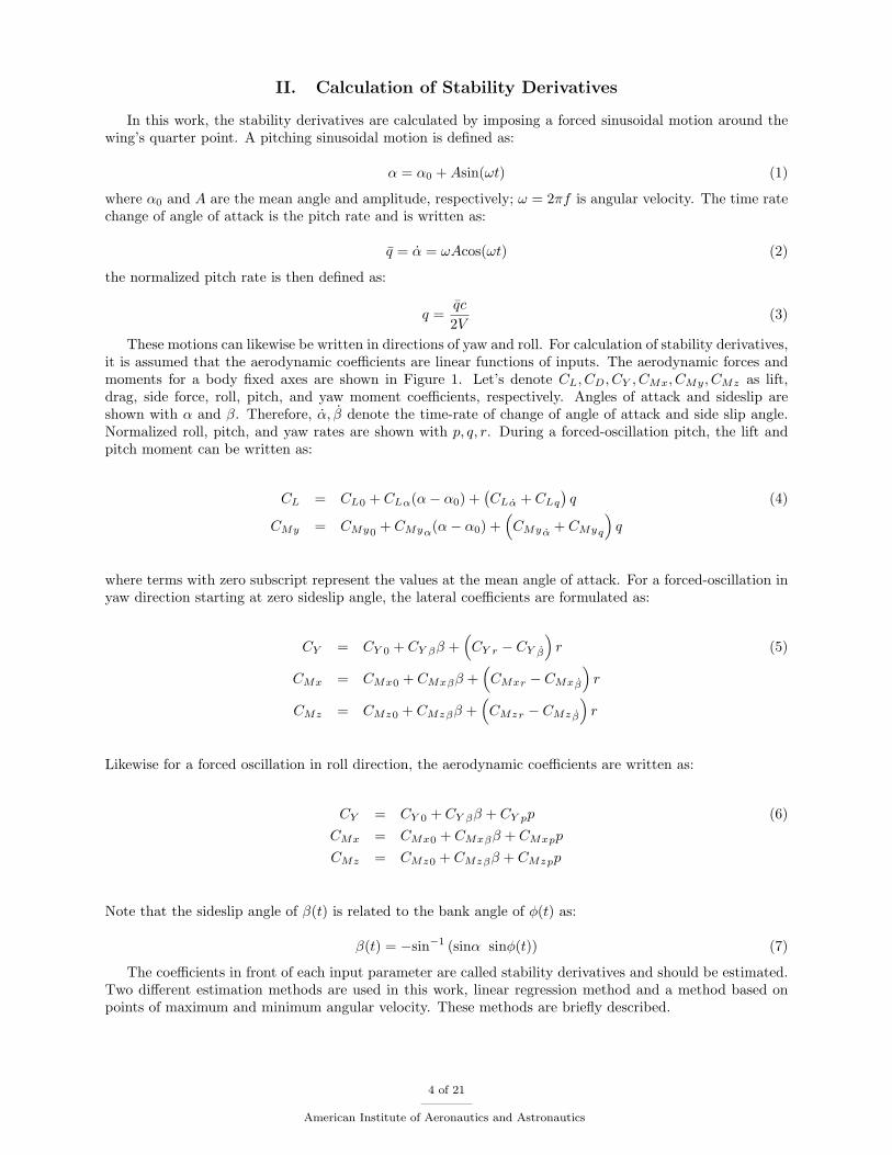
In this work, the stability derivatives are calculated by imposing a forced sinusoidal motion around thewing’s quarter point. A pitching sinusoidal motion is defined as:

α = α0 +Asin(ωt) (1)

where α0 and A are the mean angle and amplitude, respectively; ω = 2πf is angular velocity. The time ratechange of angle of attack is the pitch rate and is written as:

q̄ = α̇ = ωAcos(ωt) (2)

the normalized pitch rate is then defined as:

q =q̄c

2V(3)

These motions can likewise be written in directions of yaw and roll. For calculation of stability derivatives,it is assumed that the aerodynamic coefficients are linear functions of inputs. The aerodynamic forces andmoments for a body fixed axes are shown in Figure 1. Let’s denote CL, CD, CY , CMx, CMy, CMz as lift,drag, side force, roll, pitch, and yaw moment coefficients, respectively. Angles of attack and sideslip areshown with α and β. Therefore, α̇, β̇ denote the time-rate of change of angle of attack and side slip angle.Normalized roll, pitch, and yaw rates are shown with p, q, r. During a forced-oscillation pitch, the lift andpitch moment can be written as:

CL = CL0 + CLα(α− α0) +(CLα̇ + CLq

)q (4)

CMy = CMy0 + CMyα(α− α0) +(CMyα̇ + CMyq

)q

where terms with zero subscript represent the values at the mean angle of attack. For a forced-oscillation inyaw direction starting at zero sideslip angle, the lateral coefficients are formulated as:

CY = CY 0 + CY ββ +(CY r − CY β̇

)r (5)

CMx = CMx0 + CMxββ +(CMxr − CMxβ̇

)r

CMz = CMz0 + CMzββ +(CMzr − CMzβ̇

)r

Likewise for a forced oscillation in roll direction, the aerodynamic coefficients are written as:

CY = CY 0 + CY ββ + CY pp (6)

CMx = CMx0 + CMxββ + CMxpp

CMz = CMz0 + CMzββ + CMzpp

Note that the sideslip angle of β(t) is related to the bank angle of ϕ(t) as:

β(t) = −sin−1 (sinα sinϕ(t)) (7)

The coefficients in front of each input parameter are called stability derivatives and should be estimated.Two different estimation methods are used in this work, linear regression method and a method based onpoints of maximum and minimum angular velocity. These methods are briefly described.

4 of 21


A. Linear Regression Method

Equations 4-7 can be arranged in the form of:

y = β0 + β1x1 + β2x2 + ...+ βkxk + ϵ (8)

where y is a chosen aerodynamic coefficient; x1, x2, ..., xk are corresponding inputs; β⃗ = [β0, β1, ..., βk] is thevector of unknown coefficients for selected aerodynamic coefficient and ϵ is the approximation error. Nowassume there are n samples of function of y; define the vectors of y⃗ = [y1, y2, ..., yn] and ϵ⃗ = [ϵ1, ϵ2, ..., ϵn];In this work y⃗ contains full CFD data from forced oscillation motions and n is number of time steps.Independent inputs of x1, x2, ..., xk are the variables used in Eqs. 4-7 (e.g. α, β, ...). These variables areknown at each time step of motion. The input matrix of X is then defined as:

X =

1 x11 · · · xk1

1 x12 · · · xk2

......

......

1 x1n · · · xkn

(9)

The sum of squared errors should be minimized; the squared error is:

S =(y⃗ −XTβ⃗

)T (y⃗ −XTβ⃗

)(10)

The unknown parameters can then be estimated as:

β⃗ =(XXT

)−1(Xy⃗) (11)

B. Points of Maximum and Minimum Angular Velocity

This is a very simple method for direct calculation of dynamic derivatives (combined terms) from simu-lations of forced periodic motions. Consider the pitch moment changes during a sinusoidal pitching motion

CMy = CMy0 + CMyα(α− α0) +(CMyα̇ + CMyq

)q (12)

The plot of pitch moment versus angle of attack makes a quasi-steady elliptical hysteresis as illustratedin Fig. 2. There exists two points at which the angular velocity is maximum and minimum. These points arewhere α = α0 as shown in Fig. 2. The maximum and minimum angular velocities equal to +ωA rad/s and−ωA rad/s. Denote pitch moment values at these points as Cm+ and Cm− and substitute them in Eq. 12to find below equations:

Cm+ = CMy0 +(CMyα̇ + CMyq

) ωAc

2V(13)

Cm− = CMy0 −(CMyα̇ + CMyq

) ωAc

2V

If we subtract these equations, the pitch damping moment can be found as:

CMyα̇ + CMyq =Cm+ − Cm−

2kA(14)

where k =ωc

2Vis the reduced frequency. Other damping coefficients can be estimated in a similar fashion.

III. Flow Solvers

Cobalt and Kestrel flow solvers are used in this work. Both codes originated from the Air VehiclesUnstructured Solver (AVUS, formally known as Cobalt60) that was developed at the Air Force ResearchLaboratory (AFRL).13,14 Cobalt is now a commercial code whilst Kestrel is being developed by the U.S.Department of Defense as part of the CREATETM-AV program. More details are given below:

5 of 21


A. Cobalt Solver

The Cobalt code14 solves the unsteady, three-dimensional and compressible Navier-Stokes equations inan inertial reference frame. The ideal gas law and Sutherland’s law close the system of equations and theentire equation set is nondimensionalized by free stream density and speed of sound.14 The Navier-Stokesequations are discretised on arbitrary grid topologies using a cell-centered finite volume method. Second-order accuracy in space is achieved using the exact Riemann solver of Gottlieb and Groth,15 and least squaresgradient calculations using QR factorization. To accelerate the solution of discretized system, a point-implicitmethod using analytic first-order inviscid and viscous Jacobians. A Newtonian sub-iteration method is usedto improve time accuracy of the point-implicit method. Tomaro et al.16 converted the code from explicit toimplicit, enabling Courant-Friedrichs-Lewy numbers as high as 106. Some available turbulence models forReynolds-averaged Navier-Stokes (RANS) and delayed detached-eddy simulations (DDES) are the Spalart-Allmaras model,17 Wilcox’s k-ω model,18 and Mentor’s SST model.19

B. Kestrel Solver

Kestrel is a new DoD-developed CFD solver in the framework of CREATE Program which is funded bythe High Performance Computing Modernization Program (HPCMP). The CREATETM Program is a 12-year program, started in 2008, and is aimed at addressing the complexity of applying computationally basedengineering to improve DoD acquisition processes.20 CREATETM consists of three computationally basedengineering tool sets for design of air vehicles, ships, and radio-frequency antennae. The fixed wing analysiscode, Kestrel, is part of the Air Vehicles Project (CREATETM-AV) and is a modularized, multidisciplinary,virtual aircraft simulation tool incorporating aerodynamics, structural dynamics, kinematics, and kinetics.20

The flow solver component of Kestrel (named kCFD) solves the unsteady, three-dimensional, compressibleRANS equations on hybrid unstructured grids.21 Its foundation is based on Godunov’s first-order accurate,exact Riemann solver.22 Second-order spatial accuracy is obtained through a least squares reconstruction.The code also uses an implicit Newton sub-iteration method to improve time accuracy as well. Grismeret al13 parallelized the code, with a demonstrated linear speed-up on thousands of processors. Kestrelreceives an eXtensible Markup Language (XML) input file generated by Kestrel User Interface and storesthe solution convergence and volume results in a common data structure for later use by the Output Managercomponent. Some available turbulence models are the Spalart-Allmaras model, Spalart-Allmaras rotationcorrection (SARC), and DDES with SARC.

IV. Test Cases

The details of test cases can be found in Ref. 11. Briefly, four wings are studied. These wings haveeither an open or closed inlet and are with and without a left-side bending trailing edge. TE deflection isapproximately 45◦ as measured from the flat lower surface. These wings are named SR, BR, OpenS andOpenB representing straight/round, bent/round, open/straight, and open/bent geometries.

The airfoil section of of all wings were provided by NSRDEC and was based on a modified Clark-Y witha flat lower surface used as the cut pattern for drop tested systems.23 The wing planform is characterizedby a rectangular wing with an aspect ratio of two and zero anhedral angle. The open wings have fourteencells as well.

viscous grids are generated for the full-geometry wings. These grids are unstructured with prismaticlayers near the surfaces. Inviscid tetrahedral grids were generated by the ICEM-CFD code; these grids werethen used as a background grid by the grid generator of TRITET24,25 which builds prism layers using afrontal technique. TRITET rebuilds the viscous grid while respecting the size of the original inviscid gridfrom ICEM-CFD. The closed-wing grids have around 30 million cells and the open-wing grids contain about45 million cells. The surface grids are shown in Fig. 3. Note that grids have a left-side bending, however,the pictures of Fig. 3 are the mirror images to show the bent side and open inlets.

The static experiments of closed wings were performed in the subsonic wind tunnel of USAFA. Thisclosed-loop tunnel has an 8 ft long test section with a test section cross-section 3 ft by 3 ft. The tunnel canachieve speeds in excess of Mach 0.5. Bergeron et al.23 detailed the experimental setup and data of ram-airparachutes. The experimental Mach and Reynolds number were 0.25 and 1.4× 106. The lift and drag forcesand pitch moment coefficients were measured by an external force balance installed under the wind tunnel.

6 of 21


V. Results and Discussion

All CFD simulations were run on the Air Force Research Laboratory (AFRL) machines of Spirit andThunder with core speeds of 2.6 and 2.3 GHz. Standard viscous no-slip wall boundary conditions are usedfor the solid surfaces, with a farfield boundary condition on the outer sphere. The flow conditions and solversetup are identical in Cobalt and Kestrel flow solvers.

Closed wing simulations were performed using the SST turbulence model and ran for 2,000 time steps.Open wings ran for 6,000 time steps and used the SARC-DDES turbulence model to capture the separationbubble(s) forming and collapsing near the leading edge. Static simulations are unsteady with second orderspatial and temporal accuracy. Time step value was set to 1× 10−4 second, and two Newton sub-iterationswere used. Dynamic motion runs were made with five Newton sub-iterations to improve time accuracy ofthe point implicit method and approximate Jacobians. In all simulations, the free-stream Mach number is0.25 and the Reynolds number corresponds to 1.4 million to match experimental conditions. The momentreference point and the point of rotation are at the wing’s quarter chord.

The validation results are described first. After 2,000 time steps, the coefficient of closed wings in CFDreached a constant value. Figure 4 compares predictions with the experimental data of closed wings. Inthis figure, Kestrel and Cobalt predictions are shown as solid and dashed-dot lines, respectively. Verygood agreement is observed in all coefficients between predictions of Cobalt and Kestrel. However, the stallbehaviors do not match up. Cobalt predicts a stall around 16◦, but no stall was observed in Kestrel. Figure 4shows the preliminary experimental data from wind tunnel as well. The measurements before stall agree verywell with the predictions as seen in Fig. 4. Based on these experiments, Cobalt may have predicted the stallangle correctly. Figure 4 also shows that by pulling the trailing edge down the lift coefficient increases butthe lift curve slope remains constant. The drag increases for the bent geometry as well. The pitch momentabout the wing’s quarter point becomes more negative. The left-side bending will produce a negative side-force, a positive roll and a negative yaw moment as well. Finally, these wings have a large positive camberand therefore produce some lift at zero angle of attack. The pitch moment about the quarter chord is nearlyconstant.

The open wing simulations ran for 6,000 time steps, but some CFD solutions still show coefficient vari-ations at final time steps. Therefore, the solutions at last 500 time steps were averaged to obtain themean values. Computed and measured aerodynamic coefficients of open wings are shown in Fig. 5. Noticethat only the straight wing was tested in the wind tunnel. Figure 5 shows that again Cobalt and Kestrelcomputations reasonably match each other and experiments before stall. At some conditions, Kestrel mayoutperform Cobalt predictions. Compared with closed wings, opening the leading edge will increase the drag.The lift coefficient will stall earlier. The pitch moment curve slope will become negative. The aerodynamicnonlinearity can be seen in Fig. 5 even at small angles of attack

After validation for CFD results, the stability derivatives are calculated by imposing a forced sinusoidalmotion around the wing’s quarter point. The first motions considered are pitching oscillation with anamplitude of one degree and a reduced frequency of 0.1 starting at different angles of attack up to 10◦.Figure 6(a)-(b) show computed lift and pitch moment loops of the SR wing for oscillations about a meanangle of six degrees using Cobalt and Kestrel. The loop directions from both codes match each other; Kestrel,however, forms slightly thinner loops. The lift loops are circumvented in a clockwise direction; but counter-clockwise loops are seen for the pitch moment. Both estimation methods where used to calculate stabilityderivatives of the SR wing from these full CFD simulations. The results of the linear regression method areshown with solid lines in Fig. 6; the pitch damping derivatives are found from the points of maximum andminimum angular velocity and are shown with dashed-dot lines in Figs. 6 (e)-(f). Both methods producedvery similar result. Figure 6 shows that SR wing has nearly constant slope curve values with the angle ofattack. Pitch moment curve slope is near zero. This wing geometry has damping derivatives that remainednearly constant with angle of attack as well. Kestrel data result in smaller damping force and less negativedamping moment compared with Cobalt.

Next results present the effects of reduced frequency on calculated stability derivatives of the SR wing.Two sets of motions were generated for reduced frequencies of k = 0.1 and k = 0.05. All motions have onedegree amplitude and start at different angles of attack. These motions were simulated in Cobalt. Figure 7compares the hysteresis loops of both motions with six degrees mean angle of attack. As the reducedfrequency increases, the hysteresis effect becomes larger as seen in Fig. 7. Stability derivatives are calculatedusing linear regression method and are shown in Fig. 7 for both motions. Some variations can be seen inderivatives due to reduced frequency changes, but they are small.

7 of 21


The open wing stability derivatives were calculated from pitching harmonic motions and are comparedwith those found for the SR wing in Fig. 8. CFD data shown in the figure are Cobalt predictions. Motionsagain have one degree amplitude and have reduced frequencies of 0.1 and 0.05. Derivatives were calculatedusing the linear regression model and the method based on maximum/minimum angular velocity. The liftand pitch moment hysteresis loops at α = 6◦ can be seen in Figs. 8 (a)-(b). These loops are very differentfrom those found for the closed wing. At α = 6◦, the hysteresis loops of the open wing are thinner and havedifferent directions. Curve slopes of the open wing show significant changes with angle of attack as seen inFigs. 8 (c)-(d). The pitch moment slope of the open wing is non zero and has negative values. Figures 8(e)-(f) show that both methods produce similar results, in particular for the angle of attack ranging fromfour to eight degrees. Pitch damping derivatives of the open wing change significantly with the angle ofattack. As detailed in Ref. 23, the open wings have an eddy formed over the lower surface at small angles ofattack. The eddy becomes smaller with increasing angle of attack. At higher angles, the flow separates atthe upper surface as well. These features make aerodynamics of the open wings very nonlinear. The effectsof motion reduced frequency on damping derivatives can be seen in Figs. 8 (e)-(f). The derivatives becomefrequency-dependent at high angles of attack.

Yaw damping derivatives of the closed wing are calculated from periodic yawing motions and shown inFig. 9. The motions again have one degree sideslip amplitude and have a reduced frequency of 0.1. Referringto Eqs. 5 and 6, the derivatives with respect to sideslip angle can be found from both yawing and rollingmotions. Figure 9 compares calculated derivatives from both motions at different angles of attack. Yawing-motion derivatives are shown with solid lines; the dashed-dot lines correspond to rolling-motion derivatives.Note that during the rolling motion, the sideslip angle is related to the bank angle and the angle of attack,such that it increases with increasing the angle of attack. Figure 9 shows that calculated derivatives aredifferent using rolling and yawing motions; they become closer as the angle of attack increases. Results ofFig. 9 confirm that Cobalt and Kestrel predictions are very similar for the closed wing geometry. Finally,the stability derivatives shown in Fig. 9 slightly change with angle of attack.

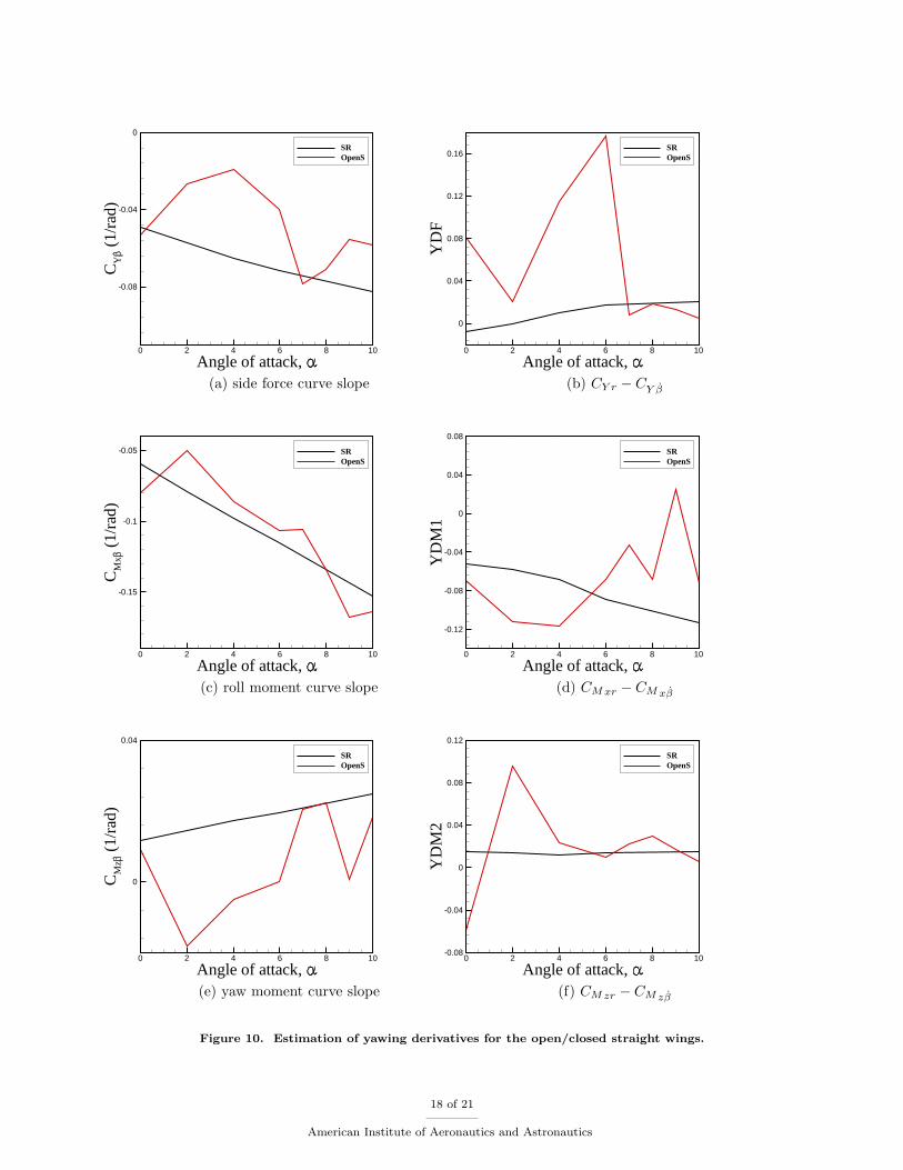
Next, the closed and open wing stability derivative during the yawing motions are compared with eachother in Fig. 10. All simulations were obtained using Cobalt. The closed wing derivatives change smoothand small with the angle of attack. However, the open wing derivatives are very sensitive to changes in theangle-of-attack. Figure 10 shows that at about 7 to 8 degrees angle of attack, the open and closed wingderivatives are closer. At these angles, a much smaller eddy is formed on the lower surface. This eddy isprobably the cause of large changes seen at small angles.

Aerodynamic derivatives with respect to rolling motions are shown in Fig. 11 for the open and closedwings. In these motions, the grids rotate about the x axis with a reduced frequency of 0.1 and one degreeamplitude. Figure 11 shows that the open wing has again a nonlinear behavior even at small angles of attack.

Damping derivatives during pitching and yawing motions have the effects of both angular velocity andunsteady effects (α̇, β̇). To separate these effects, periodic translation motions might be used. In thesemotions, the angular velocities are zero and the hysteresis loops are due to unsteady effects. To demonstratethe method, a plunging motion was applied to the open and closed wings. The motion inputs include α andα̇ but not the pitch rate. The maximum displacement was selected such that the effective angle of attackchanges from -1 to 1 around the mean angle of attack. Stability derivatives are calculated from plungingmotions and are compared with those found from the pitching motions in Fig. 12. The comparisons showthat for these wings, α̇ effects are the largest factor for pitch damping derivatives.

Since the stability derivatives are found they can be used for aerodynamic predictions of new motions.In this work, the stability derivatives models are tested for a chirp motion. The chirp motion used has aconstant amplitude and linearly increasing frequency in time. The motion is shown in Fig. 13 (a). Themodel predictions based on stability derivatives are compared with the full CFD data in Fig. 13. To showthe motion effects, the static data are also included in the plots. The comparisons show a good agreementbetween model and full CFD data for the closed wings. Static data only depend on the current angle ofattack and do not change with angular velocity. Figure 13 (d) shows that the static data underestimate themodel and CFD data for the pitch moment. There are some lag effects between static and full CFD dataas well. For the open wings, the models do not mach CFD everywhere. The comparison results show thatCFD data of the open wings are time dependent. For example, Fig. 13 (d) depicts that maximum pitchmoment coefficient obtained in CFD can increase and decrease as time progresses, although frequency doesincreases in time. These results suggest substantial unsteady effects present on the numerical simulations ofopen wings during the motion. These effects cannot be reconciled with stability derivatives.

8 of 21


VI. Concluding Remarks

This work concentrated on calculating and evaluating the stability derivative for the aerodynamic pre-dictions of ram-air parachutes with open and closed inlets. All wings were assumed to be rigid and have anaspect ratio of two. Aerodynamic predictions were made with flow solvers of Cobalt and Kestrel and werecompared with available wind-tunnel experimental data. Simulations and measurements were carried out ata Mach number of 0.25 and Reynolds number of 1.4 million.

The results showed that experimental data of wings considered here match the computational predictionsquite well. The calculated derivatives were similar for both methods and showed only a small change withreduced frequencies less than 0.1. The results showed that damping derivatives of closed wings remain fairlyconstant up to ten degrees angle of attack. However, the open wings showed a very sensitive behaviorin damping derivatives with respect to angles of attack. The models were evaluated for the closed andopen wings undergoing a chirp motion of increasing frequency. The results of the comparison showed thatthe aerodynamic models of the closed wing match time-marching full CFD calculations well, but somediscrepancies was seen in the open wing plots. These results suggested substantial unsteady effects presenton the numerical simulations of open wings during the motion. These effects cannot be reconciled withstability derivatives.

VII. Acknowledgements

Mehdi Ghoreyshi is supported by USAFA; their financial support is gratefully acknowledged. Acknowl-edgements are expressed to the Department of Defense High Performance Computing Modernization Pro-gram (HPCMP) and AFRL for providing computer time. The authors appreciate the support provided byNSRDEC Airdrop Technology Team and the High Performance Computing Research Center at USAFA.

References

1Force Multiplying Technologies for Logistics Support to Military Operations, National Academies Press, 2014.2Carter, D., Singh, L., Wholey, L., Rasmussen, S., Barrows, T., George, S., McConley, M., Gibson, C., Tavan, S., and

Bagdonovich, B., “Band-Limited Guidance and Control of Large Parafoils,” AIAA Paper 2009-2981, May 2009.3Benney, R. J., Krainski, W. J., Onckelinx, C. P., Delwarde, C. C., Mueller, L., and Vallance, M., “NATO Precision

Airdrop Initiatives and Modeling and Simulation Needs,” RTO-MP-AVT-133 Technical Report, October 2006.4Harrington, N. and Doucette, E., “Army After Next and Precision Airdrop,” Army Logistician, Vol. 31, No. 1, 1999,

pp. 46.5Mittal, S., Saxena, I. P., and Singh, A., “Computation of Two-Dimensional Flows Past Ram-Air Parachutes,” Interna-

tional Journal For Numerical Methods in Fluids, Vol. 35, 2001, pp. 643–667.6Lingard, J. S., “Precision Aerial Delivery Seminar Ram-Air Parachute Design,” 13th AIAA Aerodynamic Decelerator

Systems Technology Conference, Clearwater Beach, May 1995.7Lingard, J. S., “The Aerodynamics of Gliding Parachute,” 9th AIAA Aerodynamic Decelerator Systems Technology

Conference, AIAA Paper 1986-2427, May 1986.8Mohammadi, M. A. and Johari, H., “Computations of Flow Over a High Performance Parafoil,” AIAA Paper 2009–2972,

May 2009.9Ghoreyshi, M., Seidel, J., Bergeron, K., Lofthouse, A. J., and Cummings, R. M., “Grid Quality and Resolution Effects

on the Aerodynamic Modeling of Parachute Canopies,” AIAA Paper 2015-0407, January 2015.10Ghoreyshi, M., Seidel, J., Bergeron, K., Jirasek, A., Lofthouse, A. J., and Cummings, R. M., “Prediction of Aerodynamic

Characteristics of a Ram-Air Parachute,” AIAA Paper 2014-2831, June 2014.11Ghoreyshi, M., Bergeron, K., Jirasek, A., Seidel, J., Lofthouse, A. J., and Cummings, R. M., “Computational Aerody-

namic Modeling For Flight Dynamics Simulation of Ram-Air Parachutes,” AIAA Paper 2015-3169, June 2015.12Da Ronch, A., Vallespin, D., Ghoreyshi, M., and Badcock, K. J., “Evaluation of Dynamic Derivatives Using Computa-

tional Fluid Dynamics,” AIAA Journal, 2012.13Grismer, M. J., Strang, W. Z., Tomaro, R. F., and Witzemman, F. C., “Cobalt: A Parallel, Implicit, Unstructured

Euler/Navier-Stokes Solver,” Advanced Engineering Software, Vol. 29, No. 3-6, 1998, pp. 365–373.14Strang, W. Z., Tomaro, R. F., and Grismer, M. J., “The Defining Methods of Cobalt: A Parallel, Implicit, Unstructured

Euler/Navier-Stokes Flow Solver,” AIAA Paper 1999–0786, 1999.15Gottlieb, J. J. and Groth, C. P. T., “Assessment of Riemann Solvers For Unsteady One-dimensional Inviscid Flows of

Perfect Gasses,” Journal of Fluids and Structure, Vol. 78, No. 2, 1998, pp. 437–458.16Tomaro, R. F., Strang, W. Z., and Sankar, L. N., “An Implicit Algorithm For Solving Time Dependent Flows on

Unstructured Grids,” AIAA Paper 1997–0333, 1997.17Spalart, P. R. and Allmaras, S. R., “A One Equation Turbulence Model for Aerodynamic Flows,” AIAA Paper 1992–0439,

January 1992.

9 of 21


18Wilcox, D. C., “Reassesment of the Scale Determining Equation for Advanced Turbulence Models,” AIAA Journal ,Vol. 26, November, 1988, pp. 1299–1310.

19Menter, F., “Eddy Viscosity Transport Equations and Their Relation to the k − ε Model,” ASME Journal of FluidsEngineering, Vol. 119, 1997, pp. 876–884.

20Roth, G. L., Morton, S. A., and Brooks, G. P., “Integrating CREATE-AV Products DaVinci and Kestrel: Experiencesand Lessons Learned,” AIAA Paper 2012-1063, January 2012.

21Morton, S. A., McDaniel, D. R., Sears, D. R., Tillman, B., and Tuckey, T. R., “Kestrel: A Fixed Wing Virtual AircraftProduct of the CREATE Program,” AIAA Paper 2009-0338, January 2009.

22Godunov, S. K., “A Difference Scheme for Numerical Computation of Discontinuous Solution of Hydrodynamic Equa-tions,” Sbornik Mathematics, Vol. 47, 1959, pp. 271–306.

23Bergeron, K., Jurgen, S., and McLaughlin, T., “Wind Tunnel Investigations of Rigid Ram-Air Parachute Canopy Con-figurations,” AIAA Paper 2015–2156, March-April 2015.

24Tyssel, L., “Hybrid Grid Generation for Complex 3D Geometries,” Proceedings of the 7th International Conference onNumerical Grid Generation in Computational Field Simulation, 2000, pp. 337–346.

25Tyssel, L., “The TRITET Grid Generation System,” International Society of Grid Generation (ISGG),” Proceedings ofthe 10the International Conference on Numerical Grid Generation in Computational Field Simulations, 2000.

26Computational Research and Engineering Acquisition Tools And Environments (CREATE), Eglin AFB, FL 32542, KestrelUser Guide, Version 6.0 , August 2015.

Figure 1. Coordinate system for definition of aerodynamic forces and moments. Adapted from Ref. 26.

Angle of attack,

CM

y

5 6 7

Cm+

Cm-

Figure 2. Illustration of a method to identify pitch damping moment from points of maximum and minimumpitch rate.

10 of 21


(a) Bent and Round (BR) (b) Staright and Round (SR)

(c) Open and bent (d) Open and straight

Figure 3. Computational grids.

11 of 21


Angle of attack,

CL

0 5 10 15 200.0

0.5

1.0

1.5

Exp. (SR)Exp. (BR)CFD (SR)CFD (BR)

Angle of attack,

CD

0 5 10 15 200.0

0.1

0.2

0.3

0.4

0.5


(a) lift coefficient (b) drag coefficient

Angle of attack,

CM

y

0 5 10 15 20

-0.12

-0.08

-0.04

0.00


Angle of attack,

CY

0 5 10 15 20-0.02

-0.01

0.00

0.01

CFD (SR)CFD (BR)

(c) pitch-moment coefficient (d) side-force coefficient

Angle of attack,

CM

x

0 5 10 15 20-0.02

0.00

0.02

0.04

CFD (SR)CFD (BR)

Angle of attack,

CM

z

0 5 10 15 20-0.02

-0.01

0.00

0.01

CFD (SR)CFD (BR)

(e) roll-moment coefficient (f) yaw-force coefficient

Figure 4. Comparison of aerodynamic predictions of bent/round and straight/round wings using the SSTturbulence model.

12 of 21


Angle of attack,

CL

0 5 10 15 20

0.5

1.0 Exp. (OpenS)CFD (OpenS)CFD (OpenB)

Angle of attack,

CD

0 5 10 15 200.0

0.1

0.2

0.3

0.4

0.5

Exp. (OpenS)CFD (OpenS)CFD (OpenB)

(a) lift coefficient (b) drag coefficient

Angle of attack,

CM

y

0 5 10 15 20-0.2

-0.1

0.0

0.1Exp. (OpenS)CFD (OpenS)CFD (OpenB)

Angle of attack,

CY

0 5 10 15 20

-0.01

0.00

0.01

CFD (OpenS)CFD (OpenB)

(c) pitch-moment coefficient (d) side-force coefficient

Angle of attack,

CM

x

0 5 10 15 20-0.04

-0.02

0.00

0.02

0.04CFD (OpenS)CFD (OpenB)

Angle of attack,

CM

z

0 5 10 15 20

-0.01

0.00

0.01

CFD (OpenS)CFD (OpenB)

(e) roll-moment coefficient (f) yaw-force coefficient

Figure 5. Aerodynamic predictions of open wings.

13 of 21


Angle of attack,

CL

5 5.5 6 6.5 7

0.54

0.56

0.58

0.6

0.62 KestrelCobalt

Angle of attack,

CM

y

5 5.5 6 6.5 7-0.025

-0.02

-0.015

-0.01

KestrelCobalt

(a) lift coefficient (b) pitch moment coefficient

Angle of attack,

CL

(1/

rad)

0 2 4 6 8 10

2.6

2.8

3.0

3.2

3.4KestrelCobalt

Angle of attack,

CM

y (

1/ra

d)

0 2 4 6 8 10

-0.1

0.0

0.1

0.2KestrelCobalt

(c) lift curve slope (d) pitch moment slope

Angle of attack,

PD

F

0 2 4 6 8 10

2

4

6

8

KestrelCobalt

Angle of attack,

PD

M

0 2 4 6 8 10-2.5

-2.0

-1.5

-1.0

KestrelCobalt

(e) CLq + CLα̇ (f) CMyq + CMyα̇

Figure 6. Estimation of longitudinal derivatives for the straight/round wing. Solid and dashed lines correspondto regression and pitch rate methods, respectively.

14 of 21


Angle of attack,

CL

5 5.5 6 6.5 7

0.54

0.56

0.58

0.6

0.62 Cobalt k =0.1Cobalt k =0.05

Angle of attack,

CM

y

5 5.5 6 6.5 7-0.025

-0.02

-0.015

-0.01

Cobalt k = 0.1Cobalt K =0.05


Angle of attack,

CL

(1/

rad)

0 2 4 6 8 10

2.6

2.8

3.0

3.2

3.4 k = 0.1k = 0.05

Angle of attack,

CM

y (

1/ra

d)

0 2 4 6 8 10-0.1

0.0

0.1

0.2

k = 0.1k = 0.05

(c) lift curve slope (d) pitch moment slope

Angle of attack,

PD

F

0 2 4 6 8 102

4

6

8

10

k = 0.1k = 0.05

Angle of attack,

PD

M

0 2 4 6 8 10-6

-4

-2

0

k = 0.1k = 0.05

(e) CLq + CLα̇ (f) CMyq + CMyα̇

Figure 7. Effects of reduced frequency on pitch damping derivatives.

15 of 21


Angle of attack,

CL

5 5.5 6 6.5 70.45

0.5

0.55

0.6

SROpenS

Angle of attack,

CM

y

5 5.5 6 6.5 7-0.025

-0.02

-0.015

-0.01

-0.005

0

SROpenS


Angle of attack,

CL

(1/

rad)

0 2 4 6 8 102.0

2.5

3.0

3.5

4.0

SROpenS

Angle of attack,

CM

y (

1/ra

d)

0 2 4 6 8 10

-0.5

0.0

SROpenS

(b) lift curve slope (c) pitch moment slope

Angle of attack,

PD

F

0 2 4 6 8 10-5

0

5

10

15

20

25

SROpenS k=0.1OpenS k=0.05

Angle of attack,

PD

M

0 2 4 6 8 10-4

-2

0

2

4SROpenS k=0.1OpenS k=0.05

(d) CLq + CLα̇ (e) CMyq + CMyα̇

Figure 8. Estimation of longitudinal derivatives for the open straight and straight/round wing. Solid anddashed lines correspond to regression and pitch rate methods, respectively.

16 of 21


Angle of attack,

CY

(1/

rad)

0 2 4 6 8 10

-0.08

-0.04

0

KestrelCobaltKestrel - Rolling motionCobalt - Rolling motion

Angle of attack,

YD

F

0 2 4 6 8 10-0.04

0

0.04

KestrelCobalt

(a) side force curve slope (b) CY r − CY β̇

Angle of attack,

CM

x (

1/ra

d)

0 2 4 6 8 10

-0.1

0


Angle of attack,

YD

M1

0 2 4 6 8 10-0.12

-0.08

-0.04

0

KestrelCobalt

(c) roll moment curve slope (d) CMxr − CMxβ̇

Angle of attack,

CM

z (

1/ra

d)

0 2 4 6 8 100

0.02

0.04


Angle of attack,

YD

M2

0 2 4 6 8 100.01

0.012

0.014

0.016

KestrelCobalt

(e) yaw moment curve slope (f) CMzr − CMzβ̇

Figure 9. Estimation of yawing derivatives for the closed straight wing.

17 of 21


Angle of attack,

CY

(1/

rad)

0 2 4 6 8 10

-0.08

-0.04

0

SROpenS

Angle of attack,

YD

F

0 2 4 6 8 10

0

0.04

0.08

0.12

0.16SROpenS

(a) side force curve slope (b) CY r − CY β̇

Angle of attack,

CM

x (

1/ra

d)

0 2 4 6 8 10

-0.15

-0.1

-0.05 SROpenS

Angle of attack,

YD

M1

0 2 4 6 8 10

-0.12

-0.08

-0.04

0

0.04

0.08

SROpenS

(c) roll moment curve slope (d) CMxr − CMxβ̇

Angle of attack,

CM

z (

1/ra

d)

0 2 4 6 8 10

0

0.04

SROpenS

Angle of attack,

YD

M2

0 2 4 6 8 10-0.08

-0.04

0

0.04

0.08

0.12

SROpenS

(e) yaw moment curve slope (f) CMzr − CMzβ̇

Figure 10. Estimation of yawing derivatives for the open/closed straight wings.

18 of 21


Angle of attack,

RD

F

0 2 4 6 8 10-0.2

-0.15

-0.1

-0.05

0

SROpenS

Angle of attack,

RD

M1

0 2 4 6 8 100

0.1

0.2

0.3

0.4

0.5

0.6

SROpenS

(a) CY p (b) CMxp

Angle of attack,

RD

M2

0 2 4 6 8 10-0.1

0

0.1

0.2

0.3

SROpenS

(b) CMzp

Figure 11. Estimation of rolling derivatives for the open/closed straight wings.

19 of 21


Angle of attack,

PD

F

0 2 4 6 8 10-5

0

5

10

15

20

SR (pitching)OpenS (pitching)SR (plunging)OpenS (plunging)

Angle of attack,

PD

M

0 2 4 6 8 10-4

-2

0

2

4

6

SR (pitching)OpenS (pitching)SR (plunging)OpenS (plunging)

(a) pitching: CLq + CLα̇, plunging: CLα̇ (b) pitching: CMyq + CMyα̇, plunging: CMyα̇

Figure 12. Estimation of pitching derivatives for the open/closed straight wings from pitching/plunging mo-tions. All motions has one degree amplitude and a reduced frequency of 0.1. In plunging motions q = 0.

20 of 21


Time (s)

Ang

le o

f at

tack

,

0 0.2 0.4 0.6 0.8 1-2

0

2

4

6

8

10

(a) A chirp motion

Time (s)

CL

0 0.2 0.4 0.6 0.8 10

0.2

0.4

0.6

0.8

1

CFDStaticModel

Time (s)

CL

0 0.2 0.4 0.6 0.8 10

0.2

0.4

0.6

0.8

1

CFDStaticModel

(b) SR, lift coefficient (c) OpenS, lift coefficient

Time (s)

CM

y

0 0.2 0.4 0.6 0.8 1

-0.04

-0.02

0CFDStaticModel

Time (s)

CM

y

0 0.2 0.4 0.6 0.8 1

-0.04

-0.02

0

0.02

0.04

0.06CFDStaticModel

(d) SR, pitch moment coefficient (e) OpenS, pitch moment coefficient

Figure 13. Aerodynamic modeling of the open/closed straight wings for a chirp motions.

21 of 21


cfd calculation of stability and control derivatives for ...cfd calculation of stability and control...

Documents