Cesium Clocks: Telling Time with Spectroscopy

by

Mark Hayden

A Thesis in Chemistry Education

Presented to the Faculty of the University of Pennsylvania in partial fulfillment of the

requirement of the degree of

Master of Chemistry Education

At

University of Pennsylvania

2009

__________________________

Constance W. Blasie

Program Director

__________________________

Dr. Michael Topp

Thesis Advisor

__________________________

Hayden Page 2

1. Introduction

Due to the nature of science, all scientific disciplines depend on advancements in

metrology, the science of measurement. The quality of data is limited by the accuracy and

precision of instruments used in the data collection process. Communication and peer review

cannot occur without

established physical

quantities that are universally

accepted and accessible.

Time, length, temperature,

and mass are fundamental

quantities from which many

others can be derived.

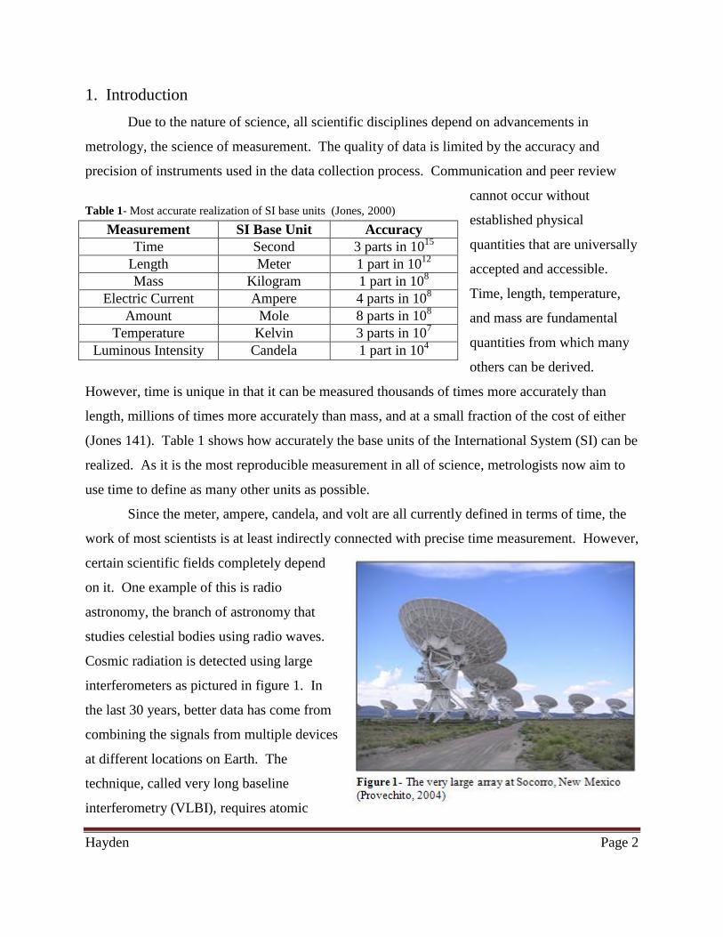
However, time is unique in that it can be measured thousands of times more accurately than

length, millions of times more accurately than mass, and at a small fraction of the cost of either

(Jones 141). Table 1 shows how accurately the base units of the International System (SI) can be

realized. As it is the most reproducible measurement in all of science, metrologists now aim to

use time to define as many other units as possible.

Since the meter, ampere, candela, and volt are all currently defined in terms of time, the

work of most scientists is at least indirectly connected with precise time measurement. However,

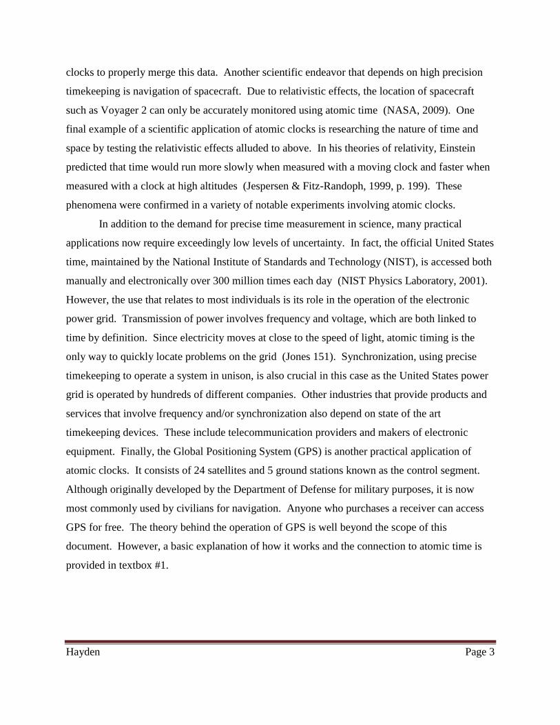
certain scientific fields completely depend

on it. One example of this is radio

astronomy, the branch of astronomy that

studies celestial bodies using radio waves.

Cosmic radiation is detected using large

interferometers as pictured in figure 1. In

the last 30 years, better data has come from

combining the signals from multiple devices

at different locations on Earth. The

technique, called very long baseline

interferometry (VLBI), requires atomic

Table 1- Most accurate realization of SI base units (Jones, 2000)

Measurement SI Base Unit Accuracy

Time Second 3 parts in 1015

Length Meter 1 part in 1012

Mass Kilogram 1 part in 108

Electric Current Ampere 4 parts in 108

Amount Mole 8 parts in 108

Temperature Kelvin 3 parts in 107

Luminous Intensity Candela 1 part in 104

Hayden Page 3

clocks to properly merge this data. Another scientific endeavor that depends on high precision

timekeeping is navigation of spacecraft. Due to relativistic effects, the location of spacecraft

such as Voyager 2 can only be accurately monitored using atomic time (NASA, 2009). One

final example of a scientific application of atomic clocks is researching the nature of time and

space by testing the relativistic effects alluded to above. In his theories of relativity, Einstein

predicted that time would run more slowly when measured with a moving clock and faster when

measured with a clock at high altitudes (Jespersen & Fitz-Randoph, 1999, p. 199). These

phenomena were confirmed in a variety of notable experiments involving atomic clocks.

In addition to the demand for precise time measurement in science, many practical

applications now require exceedingly low levels of uncertainty. In fact, the official United States

time, maintained by the National Institute of Standards and Technology (NIST), is accessed both

manually and electronically over 300 million times each day (NIST Physics Laboratory, 2001).

However, the use that relates to most individuals is its role in the operation of the electronic

power grid. Transmission of power involves frequency and voltage, which are both linked to

time by definition. Since electricity moves at close to the speed of light, atomic timing is the

only way to quickly locate problems on the grid (Jones 151). Synchronization, using precise

timekeeping to operate a system in unison, is also crucial in this case as the United States power

grid is operated by hundreds of different companies. Other industries that provide products and

services that involve frequency and/or synchronization also depend on state of the art

timekeeping devices. These include telecommunication providers and makers of electronic

equipment. Finally, the Global Positioning System (GPS) is another practical application of

atomic clocks. It consists of 24 satellites and 5 ground stations known as the control segment.

Although originally developed by the Department of Defense for military purposes, it is now

most commonly used by civilians for navigation. Anyone who purchases a receiver can access

GPS for free. The theory behind the operation of GPS is well beyond the scope of this

document. However, a basic explanation of how it works and the connection to atomic time is

provided in textbox #1.

Hayden Page 4

Textbox #1: Measurement and the Global Positioning System

All measured values are estimates that involve uncertainty. The time measurements required to operate

The Global Positioning System (GPS) carry some of the lowest uncertainties in all of science. These

measurements are made using atomic clocks.

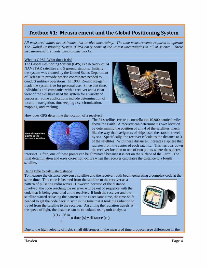
What is GPS? What does it do?

The Global Positioning System (GPS) is a network of 24

NAVSTAR satellites and 5 ground stations. Initially,

the system was created by the United States Department

of Defense to provide precise coordinates needed to

conduct military operations. In 1983, Ronald Reagan

made the system free for personal use. Since that time,

individuals and companies with a receiver and a clear

view of the sky have used the system for a variety of

purposes. Some applications include determination of

location, navigation, timekeeping / synchronization,

mapping, and tracking.

How does GPS determine the location of a receiver?

The 24 satellites create a constellation 10,900 nautical miles

above the Earth. A receiver can determine its own location

by determining the position of any 4 of the satellites, much

like the way that navigators of ships used the stars to travel

by sea. Specifically, the receiver calculates the distance to 3

of the satellites. With these distances, it creates a sphere that

radiates from the center of each satellite. This narrows down

the receiver location to one of two points where the spheres

intersect. Often, one of these points can be eliminated because it is not on the surface of the Earth. The

final determination and error correction occurs when the receiver calculates the distance to a fourth

satellite.

Using time to calculate distance

To measure the distance between a satellite and the receiver, both begin generating a complex code at the

same time. This code is beamed from the satellite to the receiver as a

pattern of pulsating radio waves. However, because of the distance

involved, the code reaching the receiver will be out of sequence with the

code that is being generated at the receiver. If both the receiver and the

satellite started releasing the pattern at the exact same time, the time-shift

needed to get the code back in sync is the time that it took the radiation to

travel from the satellite to the receiver. Assuming the radiation travels at

the speed of light, the distance can be calculated using unit analysis:

(m) distance (s) times

m103.0 8

Due to the high velocity of light, small differences in the measured time produce large differences in the

Hayden Page 5

calculated distance. Even a difference of 1/100th of a second, many times faster than the blink of an eye,

results in drastically different calculated distances as shown below:

m10 x 1.8 s 0.060 s

m103.0 m10 x 1.5 s 0.050

s

m103.0

s 0.060 t s 0.050t

78

78

1.8 x 107 m – 1.5 x 10

7 m = 3.0 x 10

6 m

Note that a difference of 1/100th of a second resulted in a difference of 3 million meters, just under half of

the radius of the Earth! In addition, large errors occur in the distance calculations if the patterns of pulses

coming from the satellite and the receiver are not synchronized initially.

Time Measurement and Synchronization

Atomic clocks are the only timing devices with the precision needed to

operate GPS. They keep track of time by mimicking periodic electron

transitions within rubidium and cesium atoms. All 24 NAVSTAR satellites

have several atomic clocks on board, each keeping time with an uncertainty

of less than 1 x 10-8

. The 5 ground stations house even better atomic clocks.

They communicate with all of the satellites and each other to ensure that the

entire system remains synchronized. Clocks at these stations have

uncertainties as low as 5 x 10-16

, meaning that they are on pace to not gain or

lose a second for over 60 million years!

References Geocachegirls.com. (2007). Ground station [Data file]. Retrieved from http://geocachegirls.com/images/grnd_station.jpg

Levine, J. (2002, July). Time and frequency distribution using satellites. Reports on progress in physics, 65, 1119-1164.

National Air and Space Museum. (1998). GPS: A new constellation. Retrieved July 26, 2009, from Smithsonian Web site:

http://www.nasm.si.edu/gps/index.htm

Navstar [Data file]. (2009). Retrieved from Enseignement polytechnique Web site: http://www.enseignement.polytechnique.fr/mecanique/

Images/Navstar-2.jpg

NIST-F1 cesium fountain atomic clock [Physics laboratory: Time and frequency division]. (n.d.). Retrieved July 20, 2009, from National Institute of Standards and Technology Web site: http://tf.nist.gov/cesium/fountain.htm

Trimble Navigation Limited. (2009). GPS tutorial. Retrieved July 26, 2009, from http://www.trimble.com/gps/index.shtml

As previously mentioned, science requires established physical quantities that are

universally accepted and accessible. These references are called standards. Today, scientists

rely on the SI units and standards adopted by the General Conference on Weights and Measures

(CGPM). However, before the first version of the current system was created in 1875,

metrologists experimented and debated over various standards. For instance, some suggested

defining the meter as a fraction of the distance of the circumference of the Earth, while others

preferred using the length of a pendulum with a particular period (NIST, 2009). Ultimately, the

Hayden Page 6

former was used due to fluctuations in the pendulum’s period at different places on Earth. Using

this calculated distance, a platinum-iridium bar was made in 1889 to serve as the standard of

length. Copies of this standard were distributed to various countries. A similar standard with

copies was created for the kilogram.

Examples of both standards are shown in

figure 2. However, a similar standard was

not available for the second. The quest to

establish a “physical second” was the

driving force behind much of the

foundational research and developments

made in atomic timekeeping. By 1967,

the international scientific community was sufficiently satisfied with the accuracy, stability, and

reproducibility of the cesium clock and defined the second using the frequency of a specific

electronic transition within cesium. Rapid developments in atomic time continue to this day with

6 of the 7 base SI units, including the meter, now redefined in terms of the second. Although the

kilogram standard is still a platinum-iridium mass, many are in favor of redefining it in terms of

the second using the speed of light in Einstein’s famous equation (Jones 159):

E = mc2

(1)

2. Timekeeping and Frequency

Historical Clocks

Timekeeping involves counting and keeping track of cycles of a repetitive event.

Throughout history, this has been done in a variety of ways involving a broad spectrum of

sophistication. Periodic astronomical occurrences, especially the spin of the Earth and its

rotation around the sun, have long served as the repetitive event used to keep track of time.

Surely, even our earliest ancestors were able to count days simply by acknowledging the

repeating cycle of light and darkness. As early as 3500 B.C., Egyptians had developed obelisks

that could be used to divide the day into 12 parts (Jespersen & Fitz-Randoph, 1999, p. 11).

Solar timekeepers realized that the length of a day varies when measured using the

position of the sun in the sky. The combination of the Earth’s elliptical orbit, varying orbit

speed, and tilted axis produce a complex variation in the length of the solar day. This leads to a

Hayden Page 7

difference in nearly a full minute depending on the month. Although methods were developed to

correct sundials and other timekeeping devices for these factors, time cannot be measured

precisely on the basis of a day that is not constant. For this reason, astronomers developed the

“mean solar day.” It is a more convenient average value for the day that assumes that the sun’s

orbit in the sky as seen from Earth is consistent. It is essentially a mathematical correction for

the variations listed above (Jones, 2000, p. 5). For centuries, the second was defined as

1/86,400 of the mean solar day (Time Services Department, 2003):

(2)

Meanwhile, many were less interested in correcting solar clocks and more interested in

developing accurate timekeeping devices on Earth. Not only were these devices more accurate

than sundials and more useful for monitoring small increments of time, but they also could be

used on cloudy days or at night. The Egyptians, Chinese, Greeks, and Romans built

sophisticated sand and water clocks. However, because of a variety of problems with these

devices, the focus was shifted almost entirely to mechanical clocks by the start of the 15th

century (Jespersen & Fitz-Randoph, 1999, p. 36). Although many types of mechanical clocks

were constructed, few made more of an impact than the pendulum clock.

Galileo is generally credited with coming up with the idea of using a pendulum as the

repetitive event from which to keep time, although he did not construct a working device before

his death in 1642. Christiaan Huygens, known for his work in mathematics and physics, is

credited with developing the first working pendulum clock, which he patented in 1657. Initial

models of this clock were accurate within 10 seconds a day, which was a drastic improvement

over other clocks from the past (Jespersen & Fitz-Randoph, 1999, p. 37). However, it was a

new version of the pendulum clock, called the Shortt clock, which made the biggest impact in

science.

Hayden Page 8

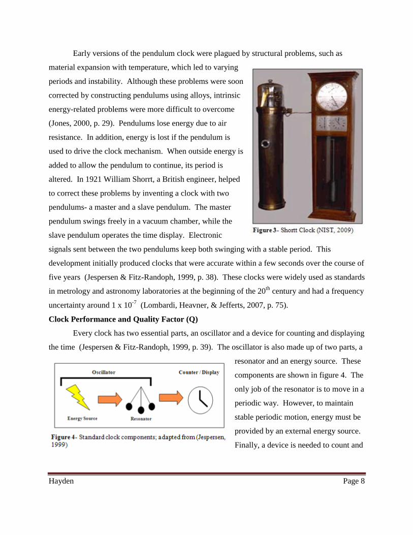
Early versions of the pendulum clock were plagued by structural problems, such as

material expansion with temperature, which led to varying

periods and instability. Although these problems were soon

corrected by constructing pendulums using alloys, intrinsic

energy-related problems were more difficult to overcome

(Jones, 2000, p. 29). Pendulums lose energy due to air

resistance. In addition, energy is lost if the pendulum is

used to drive the clock mechanism. When outside energy is

added to allow the pendulum to continue, its period is

altered. In 1921 William Shorrt, a British engineer, helped

to correct these problems by inventing a clock with two

pendulums- a master and a slave pendulum. The master

pendulum swings freely in a vacuum chamber, while the

slave pendulum operates the time display. Electronic

signals sent between the two pendulums keep both swinging with a stable period. This

development initially produced clocks that were accurate within a few seconds over the course of

five years (Jespersen & Fitz-Randoph, 1999, p. 38). These clocks were widely used as standards

in metrology and astronomy laboratories at the beginning of the 20th

century and had a frequency

uncertainty around 1 x 10-7

(Lombardi, Heavner, & Jefferts, 2007, p. 75).

Clock Performance and Quality Factor (Q)

Every clock has two essential parts, an oscillator and a device for counting and displaying

the time (Jespersen & Fitz-Randoph, 1999, p. 39). The oscillator is also made up of two parts, a

resonator and an energy source. These

components are shown in figure 4. The

only job of the resonator is to move in a

periodic way. However, to maintain

stable periodic motion, energy must be

provided by an external energy source.

Finally, a device is needed to count and

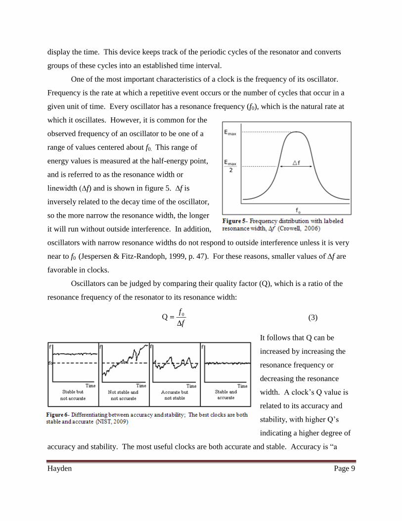
Hayden Page 9

display the time. This device keeps track of the periodic cycles of the resonator and converts

groups of these cycles into an established time interval.

One of the most important characteristics of a clock is the frequency of its oscillator.

Frequency is the rate at which a repetitive event occurs or the number of cycles that occur in a

given unit of time. Every oscillator has a resonance frequency (f0), which is the natural rate at

which it oscillates. However, it is common for the

observed frequency of an oscillator to be one of a

range of values centered about f0. This range of

energy values is measured at the half-energy point,

and is referred to as the resonance width or

linewidth (∆f) and is shown in figure 5. ∆f is

inversely related to the decay time of the oscillator,

so the more narrow the resonance width, the longer

it will run without outside interference. In addition,

oscillators with narrow resonance widths do not respond to outside interference unless it is very

near to f0 (Jespersen & Fitz-Randoph, 1999, p. 47). For these reasons, smaller values of ∆f are

favorable in clocks.

Oscillators can be judged by comparing their quality factor (Q), which is a ratio of the

resonance frequency of the resonator to its resonance width:

f

f 0Q (3)

It follows that Q can be

increased by increasing the

resonance frequency or

decreasing the resonance

width. A clock’s Q value is

related to its accuracy and

stability, with higher Q’s

indicating a higher degree of

accuracy and stability. The most useful clocks are both accurate and stable. Accuracy is “a

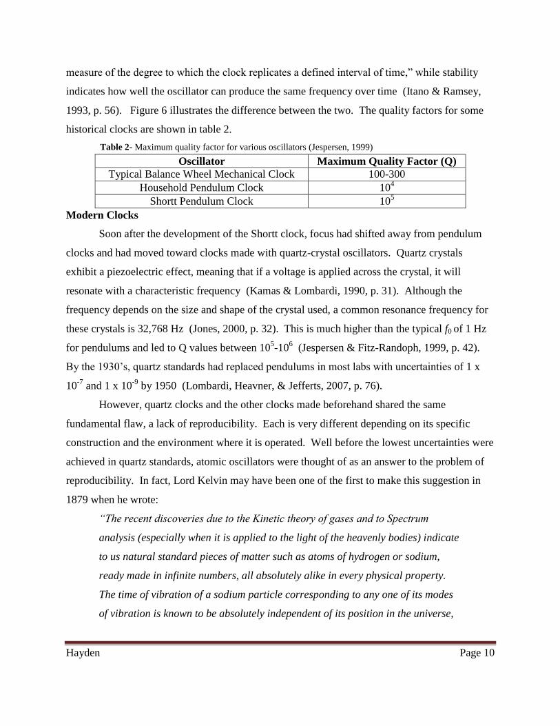
Hayden Page 10

measure of the degree to which the clock replicates a defined interval of time,” while stability

indicates how well the oscillator can produce the same frequency over time (Itano & Ramsey,

1993, p. 56). Figure 6 illustrates the difference between the two. The quality factors for some

historical clocks are shown in table 2.

Table 2- Maximum quality factor for various oscillators (Jespersen, 1999)

Oscillator Maximum Quality Factor (Q)

Typical Balance Wheel Mechanical Clock 100-300

Household Pendulum Clock 104

Shortt Pendulum Clock 105

Modern Clocks

Soon after the development of the Shortt clock, focus had shifted away from pendulum

clocks and had moved toward clocks made with quartz-crystal oscillators. Quartz crystals

exhibit a piezoelectric effect, meaning that if a voltage is applied across the crystal, it will

resonate with a characteristic frequency (Kamas & Lombardi, 1990, p. 31). Although the

frequency depends on the size and shape of the crystal used, a common resonance frequency for

these crystals is 32,768 Hz (Jones, 2000, p. 32). This is much higher than the typical f0 of 1 Hz

for pendulums and led to Q values between 105-10

6 (Jespersen & Fitz-Randoph, 1999, p. 42).

By the 1930’s, quartz standards had replaced pendulums in most labs with uncertainties of 1 x

10-7

and 1 x 10-9

by 1950 (Lombardi, Heavner, & Jefferts, 2007, p. 76).

However, quartz clocks and the other clocks made beforehand shared the same

fundamental flaw, a lack of reproducibility. Each is very different depending on its specific

construction and the environment where it is operated. Well before the lowest uncertainties were

achieved in quartz standards, atomic oscillators were thought of as an answer to the problem of

reproducibility. In fact, Lord Kelvin may have been one of the first to make this suggestion in

1879 when he wrote:

“The recent discoveries due to the Kinetic theory of gases and to Spectrum

analysis (especially when it is applied to the light of the heavenly bodies) indicate

to us natural standard pieces of matter such as atoms of hydrogen or sodium,

ready made in infinite numbers, all absolutely alike in every physical property.

The time of vibration of a sodium particle corresponding to any one of its modes

of vibration is known to be absolutely independent of its position in the universe,

Hayden Page 11

and will probably remain the same so long as the particle itself exists” (Jones,

2000, p. 33).

Atomic clocks were only possible after substantial developments in quantum mechanics

and microwave technologies made before, during, and after the second world war (Diddams,

Bergquist, Jefferts, & Oates, 2004, p. 1319). Quantum mechanics suggests that atoms only

absorb and release energy in discrete amounts called quanta. Theoretically, the resonance

frequency of an atom depends on differences between allowed energy levels as shown in

equation 4, where h is Planck’s constant:

h

EEf 12

0 (4)

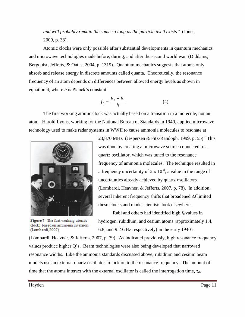
The first working atomic clock was actually based on a transition in a molecule, not an

atom. Harold Lyons, working for the National Bureau of Standards in 1949, applied microwave

technology used to make radar systems in WWII to cause ammonia molecules to resonate at

23,870 MHz (Jespersen & Fitz-Randoph, 1999, p. 55). This

was done by creating a microwave source connected to a

quartz oscillator, which was tuned to the resonance

frequency of ammonia molecules. The technique resulted in

a frequency uncertainty of 2 x 10-8

, a value in the range of

uncertainties already achieved by quartz oscillators

(Lombardi, Heavner, & Jefferts, 2007, p. 78). In addition,

several inherent frequency shifts that broadened ∆f limited

these clocks and made scientists look elsewhere.

Rabi and others had identified high f0 values in

hydrogen, rubidium, and cesium atoms (approximately 1.4,

6.8, and 9.2 GHz respectively) in the early 1940’s

(Lombardi, Heavner, & Jefferts, 2007, p. 79). As indicated previously, high resonance frequency

values produce higher Q’s. Beam technologies were also being developed that narrowed

resonance widths. Like the ammonia standards discussed above, rubidium and cesium beam

models use an external quartz oscillator to lock on to the resonance frequency. The amount of

time that the atoms interact with the external oscillator is called the interrogation time, τd.

Hayden Page 12

Quality factors are inversely related to τd as shown in the following relationship (Lombardi,

Heavner, & Jefferts, 2007, p. 79):

00

1

ff d

f (5)

The combination of higher f0 and lower ∆f values for atomic resonators produce much higher-Q

values and more accurate and stable clocks.

Table 3- Maximum quality factor for additional oscillators (Jespersen, 1999)

Oscillator Maximum Quality Factor (Q)

Quartz clock 105-10

6

Rubidium clock 106

Hydrogen maser 109

Cesium clock 1010

Although rubidium clocks and clocks built around hydrogen masers have advantages and

disadvantages, it is the cesium transition that is the basis of the best atomic clocks and frequency

standards used today. This is mainly due to some important properties of cesium that are

discussed in section 3. However, both the rubidium and hydrogen models are plagued by

frequency shifts and other problems that limit the time that they can operate effectively.

Defining the Second

With advancements in timekeeping and astronomy came the realization that complexities

surrounding the Earth’s rotation about its axis meant that the mean solar day should no longer

serve as the basis for determining the length of the second. Astronomers had already adopted a

new time scale called Ephemeris Time in 1952, which was based on Earth’s orbit around the sun.

In 1956, the International Committee on Weights and Measures suggested that the second should

be defined as 1/31 556 925.9747 of year 1900

(Bergquist, Jefferts, & Wineland, 2001, p. 37).

This definition was ultimately adopted by the

General Conference on Weights and Measures

in 1960.

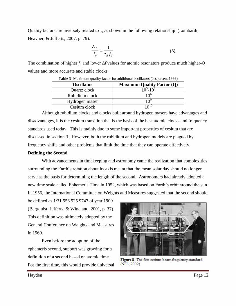
Even before the adoption of the

ephemeris second, support was growing for a

definition of a second based on atomic time.

For the first time, this would provide universal

Hayden Page 13

access to a “physical second” that did not require complex and timely astronomical observations

and calculations. In 1955, Louis Essen and Jack Parry created the first operational cesium clock,

shown in figure 8, at the National Physical Laboratory in the UK. Once reliable cesium

standards became more common, effort was directed toward determining the resonance

frequency of cesium in relation to the ephemeris second. In 1958, this was completed and the

frequency was published as 9 192 631 770 ± 20 Hz (Markowitz, Hall, Essen, & Parry, 1958, p.

107). Finally, in 1967 at the 13th

Conference on Weights and Measures, the SI second was

defined as:

“ the duration of 9 192 631 770 periods of the radiation corresponding to the

transition between the two hyperfine levels of the ground state of the cesium 133

atom.”

In 1997, it was amended to state:

“a cesium atom at rest at a thermodynamic temperature of 0K”

3. Properties of Cesium

Physical Properties

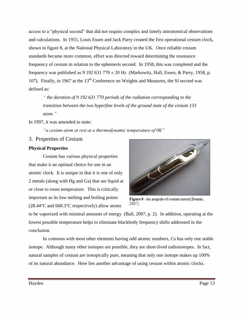
Cesium has various physical properties

that make it an optimal choice for use in an

atomic clock. It is unique in that it is one of only

2 metals (along with Hg and Ga) that are liquid at

or close to room temperature. This is critically

important as its low melting and boiling points

(28.44°C and 668.3°C respectively) allow atoms

to be vaporized with minimal amounts of energy (Ball, 2007, p. 2). In addition, operating at the

lowest possible temperature helps to eliminate blackbody frequency shifts addressed in the

conclusion.

In common with most other elements having odd atomic numbers, Cs has only one stable

isotope. Although many other isotopes are possible, they are short-lived radioisotopes. In fact,

natural samples of cesium are isotopically pure, meaning that only one isotope makes up 100%

of its natural abundance. Here lies another advantage of using cesium within atomic clocks.

Hayden Page 14

Any sample used will contain only 133

Cs, which eliminates concern about the presence of

transitions from other isotopes (Jones, 2000, p. 40).

With stable atoms having 55 protons and 78 neutrons, cesium is a heavy atom. This

limits the speed at which the atoms can travel. In fact, cesium atoms move at just greater than

8% of the speed of hydrogen atoms (130 m/s vs. 1600 m/s) at room temperature (Lombardi,

Heavner, & Jefferts, 2007, p. 79). Slower moving atoms help to increase interrogation time in

the microwave cavity. Longer interaction times lead to narrower Δfa, which in turn increase the

Q factor. Higher Q factors are associated with more accurate and stable oscillators as addressed

in section 2 (Lombardi, Heavner, & Jefferts, 2007, p. 77).

Hayden Page 15

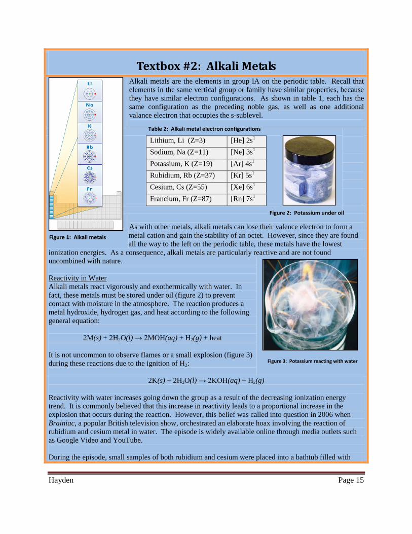
Textbox #2: Alkali Metals Alkali metals are the elements in group IA on the periodic table. Recall that

elements in the same vertical group or family have similar properties, because

they have similar electron configurations. As shown in table 1, each has the

same configuration as the preceding noble gas, as well as one additional

valance electron that occupies the s-sublevel.

As with other metals, alkali metals can lose their valence electron to form a

metal cation and gain the stability of an octet. However, since they are found

all the way to the left on the periodic table, these metals have the lowest

ionization energies. As a consequence, alkali metals are particularly reactive and are not found

uncombined with nature.

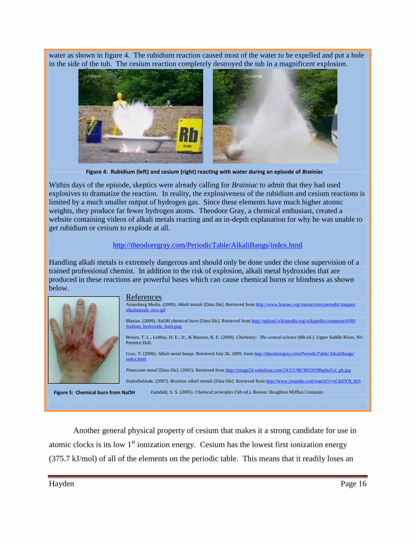
Reactivity in Water

Alkali metals react vigorously and exothermically with water. In

fact, these metals must be stored under oil (figure 2) to prevent

contact with moisture in the atmosphere. The reaction produces a

metal hydroxide, hydrogen gas, and heat according to the following

general equation:

2M(s) + 2H2O(l) → 2MOH(aq) + H2(g) + heat

It is not uncommon to observe flames or a small explosion (figure 3)

during these reactions due to the ignition of H2:

2K(s) + 2H2O(l) → 2KOH(aq) + H2(g)

Reactivity with water increases going down the group as a result of the decreasing ionization energy

trend. It is commonly believed that this increase in reactivity leads to a proportional increase in the

explosion that occurs during the reaction. However, this belief was called into question in 2006 when

Brainiac, a popular British television show, orchestrated an elaborate hoax involving the reaction of

rubidium and cesium metal in water. The episode is widely available online through media outlets such

as Google Video and YouTube.

During the episode, small samples of both rubidium and cesium were placed into a bathtub filled with

Lithium, Li (Z=3) [He] 2s1

Sodium, Na (Z=11) [Ne] 3s1

Potassium, K (Z=19) [Ar] 4s1

Rubidium, Rb (Z=37) [Kr] 5s1

Cesium, Cs (Z=55) [Xe] 6s1

Francium, Fr (Z=87) [Rn] 7s1

Figure 1: Alkali metals

Table 2: Alkali metal electron configurations

Figure 2: Potassium under oil

Figure 3: Potassium reacting with water

Hayden Page 16

water as shown in figure 4. The rubidium reaction caused most of the water to be expelled and put a hole

in the side of the tub. The cesium reaction completely destroyed the tub in a magnificent explosion.

Within days of the episode, skeptics were already calling for Brainiac to admit that they had used

explosives to dramatize the reaction. In reality, the explosiveness of the rubidium and cesium reactions is

limited by a much smaller output of hydrogen gas. Since these elements have much higher atomic

weights, they produce far fewer hydrogen atoms. Theodore Gray, a chemical enthusiast, created a

website containing videos of alkali metals reacting and an in-depth explanation for why he was unable to

get rubidium or cesium to explode at all.

http://theodoregray.com/PeriodicTable/AlkaliBangs/index.html

Handling alkali metals is extremely dangerous and should only be done under the close supervision of a

trained professional chemist. In addition to the risk of explosion, alkali metal hydroxides that are

produced in these reactions are powerful bases which can cause chemical burns or blindness as shown

below.

References Annenberg Media. (2009). Alkali metals [Data file]. Retrieved from http://www.learner.org/interactives/periodic/images/

alkalimetals_new.gif

Blazius. (2009). NaOH chemical burn [Data file]. Retrieved from http://upload.wikimedia.org/wikipedia/commons/0/09/

Sodium_hydroxide_burn.png

Brown, T. L., LeMay, H. E., Jr., & Bursten, B. E. (2000). Chemistry: The central science (8th ed.). Upper Saddle River, NJ:

Prentice Hall.

Gray, T. (2006). Alkali metal bangs. Retrieved July 26, 2009, from http://theodoregray.com/PeriodicTable/AlkaliBangs/

index.html

Potassium metal [Data file]. (2002). Retrieved from http://image24.webshots.com/24/2/1/90/38520190qdwZyi_ph.jpg

Stattotheblade. (2007). Brainiac alkali metals [Data file]. Retrieved from http://www.youtube.com/watch?v=eCk0lYB_8c0

Zumdahl, S. S. (2005). Chemical principles (5th ed.). Boston: Houghton Mifflan Company.

Another general physical property of cesium that makes it a strong candidate for use in

atomic clocks is its low 1st ionization energy. Cesium has the lowest first ionization energy

(375.7 kJ/mol) of all of the elements on the periodic table. This means that it readily loses an

Figure 4: Rubidium (left) and cesium (right) reacting with water during an episode of Brainiac

Figure 5: Chemical burn from NaOH

Hayden Page 17

electron after an input of only a minimal amount of energy. This has a practical application to

atomic clocks, because the detectors that are used in many older and commercially available

cesium-beam standards use a hot metal filament to ionize cesium atoms and generate an electric

current (Itano & Ramsey, 1993, p. 59). Types of detectors are presented in section 4.

Hyperfine Structure

Another advantage of using cesium

in atomic clocks is that it has a large nuclear

spin (I=7/2) and nuclear magnetic moment

that interact with its lone 6s1 electron

resulting in what is referred to as hyperfine

structure (Ball, 2007, pp. 2-3). Nuclei that

have an odd mass number have a non-zero

spin that results from the spin pairings of

protons and neutrons. These interactions

were studied extensively, particularly at

Columbia University, in the 1930’s by Rabi,

Cohen, Millman, Zacharias, and others

(Millman & Zacharias, 1937, p. 1049).

Zacharias is generally credited with coming

up with concept and design of the first

cesium atomic fountain which will be

discussed in section 5.

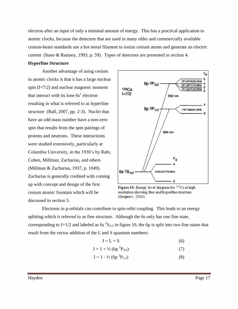
Electrons in p-orbitals can contribute to spin-orbit coupling. This leads to an energy

splitting which is referred to as fine structure. Although the 6s only has one fine state,

corresponding to J=1/2 and labeled as 6s 2S1/2 in figure 10, the 6p is split into two fine states that

result from the vector addition of the L and S quantum numbers:

J = L + S (6)

J = 1 + ½ (6p 2P3/2) (7)

J = 1 - ½ (6p 2P1/2) (8)

Hayden Page 18

In the presence of a magnetic field, such the one created by cesium’s magnetic nucleus,i

additional energy splitting called hyperfine structure can be detected at high resolution. This

splitting is the result of the vector addition of the nuclear spin (I=7/2) with J and leads to levels

labeled as F (M. Topp, personal communication, July 16, 2009):

F = I + J (9)

F = 7/2 + ½ = 4 (10)

F = 7/2 – ½ = 3 (11)

Similar hyperfine splitting occurs for the p-orbitals, with additional F values possible because of

the various combinations that result due to the presence of 3 orbital types. Each may also be

split into magnetic (mf) states in the presence of an external field.

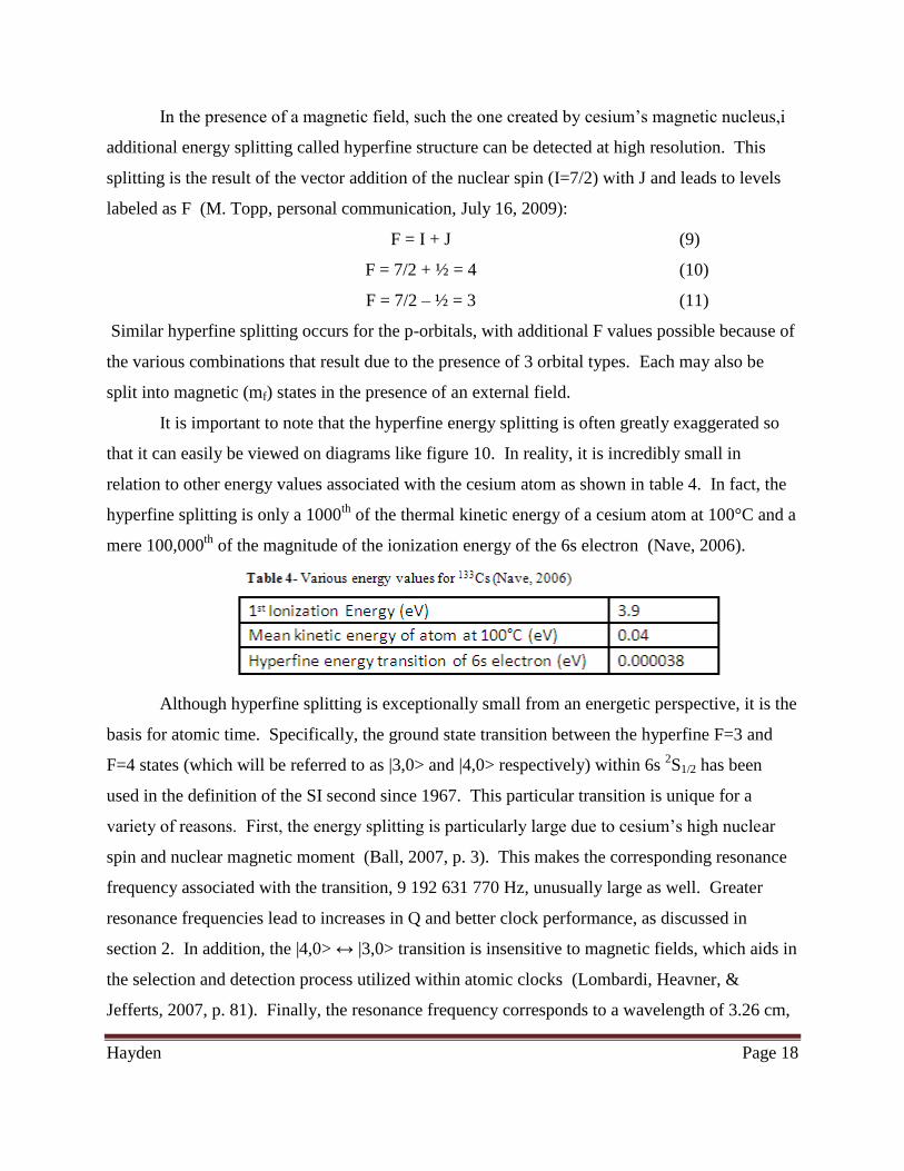
It is important to note that the hyperfine energy splitting is often greatly exaggerated so

that it can easily be viewed on diagrams like figure 10. In reality, it is incredibly small in

relation to other energy values associated with the cesium atom as shown in table 4. In fact, the

hyperfine splitting is only a 1000th

of the thermal kinetic energy of a cesium atom at 100°C and a

mere 100,000th

of the magnitude of the ionization energy of the 6s electron (Nave, 2006).

Although hyperfine splitting is exceptionally small from an energetic perspective, it is the

basis for atomic time. Specifically, the ground state transition between the hyperfine F=3 and

F=4 states (which will be referred to as |3,0> and |4,0> respectively) within 6s 2S1/2 has been

used in the definition of the SI second since 1967. This particular transition is unique for a

variety of reasons. First, the energy splitting is particularly large due to cesium’s high nuclear

spin and nuclear magnetic moment (Ball, 2007, p. 3). This makes the corresponding resonance

frequency associated with the transition, 9 192 631 770 Hz, unusually large as well. Greater

resonance frequencies lead to increases in Q and better clock performance, as discussed in

section 2. In addition, the |4,0> ↔ |3,0> transition is insensitive to magnetic fields, which aids in

the selection and detection process utilized within atomic clocks (Lombardi, Heavner, &

Jefferts, 2007, p. 81). Finally, the resonance frequency corresponds to a wavelength of 3.26 cm,

Hayden Page 19

which is part of the microwave region of the electromagnetic spectrum. Equipment is readily

available to induce and detect this transition. In fact, many of the original parts used in clocks

came from advancements made in microwave technology that was used for radar and

communication during the World War II (Diddams, Bergquist, Jefferts, & Oates, 2004, p. 2).

4. Cesium-Beam Frequency Standard

Overview

As discussed in section 2, all clocks consist of two basic components: an oscillator and a

device that counts and displays the time. Once this external source of radiation (usually a quartz

oscillator) has been tuned to match the resonance frequency of a beam of cesium atoms, a

counter keeps track of the cycles. This is very similar to the way the master and slave

pendulums operate in the Shortt clock. Cesium beam standards are no longer used as official

primary frequency standards but are still used in commercially available devices.

The process specifically involves the ground-state |4,0> ↔ |3,0> hyperfine transition in

133Cs. The frequency of the radiation absorbed and released during this transition is referred to

as the resonance frequency and has been identified as 9 192 631 770 ±20 Hz. The corresponding

wavelength is 3.26 cm, which falls in the microwave region of the electromagnetic spectrum.

The goal is to monitor and match the frequency of the external source of microwaves with the

resonance frequency of the cesium atoms.

The source of the cesium beam is an oven where a sample of cesium atoms is converted

to the gaseous state. Since cesium has a relatively low boiling point (28.4°C) and high vapor

pressure, temperatures between 80°C-100°C are enough to produce more than enough vaporized

cesium for the process (Ball, 2007, p. 2). A small slit in the side of the oven releases a beam of

the atoms. Upon leaving the oven, both ground level hyperfine states will be populated

according to the Bolzmann distribution, with F=3 slightly favored (M. Topp, personal

communication, July 21, 2009). However, all 16 possible mf states in the ground level are

occupied, 9 for F=4 and 7 for F=3 (Sullivan et al., 2001, p. 49). Even if the external source of

radiation is properly tuned to the resonance frequency, these atoms will not undergo the desired

|4,0> ↔ |3,0> transition, which makes them useless in their current states.

Hayden Page 20

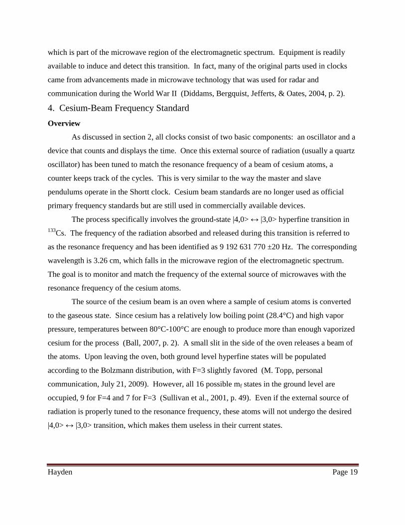
For this reason, a variety of state selection techniques are used to ensure that as many atoms as

possible are in the |3,0> hyperfine state before exposure to the microwaves. In figure 11,

magnets are used (labeled A magnet) to filter out atoms in undesirable magnetic states before

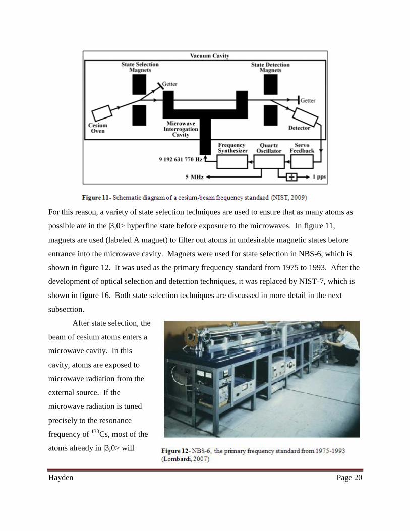
entrance into the microwave cavity. Magnets were used for state selection in NBS-6, which is

shown in figure 12. It was used as the primary frequency standard from 1975 to 1993. After the

development of optical selection and detection techniques, it was replaced by NIST-7, which is

shown in figure 16. Both state selection techniques are discussed in more detail in the next

subsection.

After state selection, the

beam of cesium atoms enters a

microwave cavity. In this

cavity, atoms are exposed to

microwave radiation from the

external source. If the

microwave radiation is tuned

precisely to the resonance

frequency of 133

Cs, most of the

atoms already in |3,0> will

Hayden Page 21

undergo a transition to |4,0>. These altered atoms are detected outside of the microwave cavity.

The number of |4,0> atoms at the detector reaches a maximum when the resonance frequency is

matched, so the frequency of the microwave radiation must be carefully adjusted until that

occurs. In the past, operators of the standard completed this meticulous process by hand.

However, modern standards employ Servo loops that electronically adjust the frequency in the

microwave cavity based on information provided by the detector. Both microwave cavities and

detectors are discussed in more depth in subsequent subsections.

State Selection Techniques

As indicated in section 3, various levels of fine (J) and hyperfine (F) structure are

detected in cesium at high resolution. In addition to these levels, magnetic (mf) splitting occurs

in the presence of an external

magnetic field. When gaseous

cesium atoms leave the oven,

they occupy all 16 of the

possible mf states within the 6s

2S1/2 ground level state

(Sullivan et al., 2001, p. 49).

These states are shown in figure

13. Both magnetic states

involved in the clock transition,

|3,0> and |4,0>, are insensitive to magnetic fields, which means that magnets can be used to

select for them (Lombardi, Heavner, & Jefferts, 2007, p. 81). In practice, the process is more

about selecting against the other 14 magnetically sensitive states. A device called a Stern-

Gerlach magnet allows atoms in the |3,0> and |4,0> to proceed toward the microwave cavity,

while deflecting atoms in other states toward a getter. However, it is still possible for atoms in

the wrong state to make it past the initial magnet. For this reason, another magnet is used to

select for the |4,0> after the microwave cavity and before detection.

Magnetic selection techniques are no longer used in the most accurate atomic clocks.

Clocks utilizing them experience an excessive amount of “noise” at their detector because of the

number of atoms in the wrong magnetic state that are able to pass by state selection magnets.

Hayden Page 22

This decreases detection efficiency and increases the amount of time needed to make

measurements. In addition, magnets have varying effects on atoms that are traveling at different

velocities, which can make the frequency distribution of the cesium atoms asymmetric (Sullivan

et al., 2001, p. 50). An asymmetric complicates the determination of the resonance frequency.

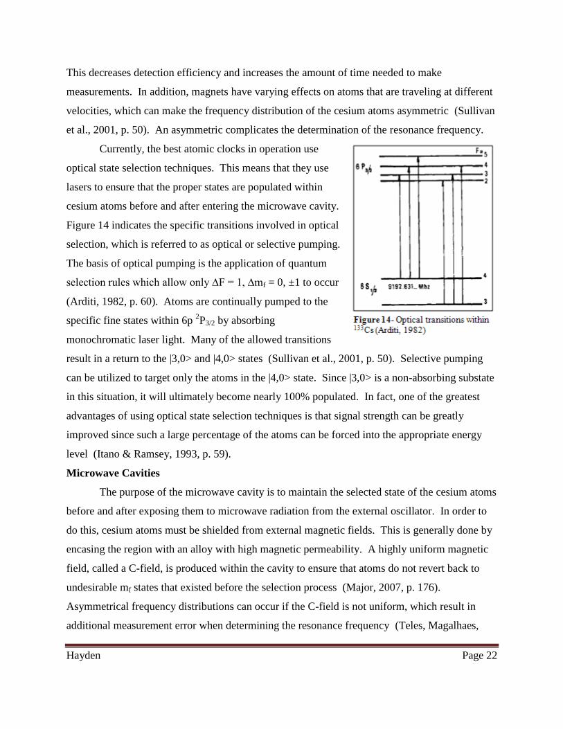
Currently, the best atomic clocks in operation use

optical state selection techniques. This means that they use

lasers to ensure that the proper states are populated within

cesium atoms before and after entering the microwave cavity.

Figure 14 indicates the specific transitions involved in optical

selection, which is referred to as optical or selective pumping.

The basis of optical pumping is the application of quantum

selection rules which allow only ∆F = 1, ∆mf = 0, ±1 to occur

(Arditi, 1982, p. 60). Atoms are continually pumped to the

specific fine states within 6p 2P3/2 by absorbing

monochromatic laser light. Many of the allowed transitions

result in a return to the |3,0> and |4,0> states (Sullivan et al., 2001, p. 50). Selective pumping

can be utilized to target only the atoms in the |4,0> state. Since |3,0> is a non-absorbing substate

in this situation, it will ultimately become nearly 100% populated. In fact, one of the greatest

advantages of using optical state selection techniques is that signal strength can be greatly

improved since such a large percentage of the atoms can be forced into the appropriate energy

level (Itano & Ramsey, 1993, p. 59).

Microwave Cavities

The purpose of the microwave cavity is to maintain the selected state of the cesium atoms

before and after exposing them to microwave radiation from the external oscillator. In order to

do this, cesium atoms must be shielded from external magnetic fields. This is generally done by

encasing the region with an alloy with high magnetic permeability. A highly uniform magnetic

field, called a C-field, is produced within the cavity to ensure that atoms do not revert back to

undesirable mf states that existed before the selection process (Major, 2007, p. 176).

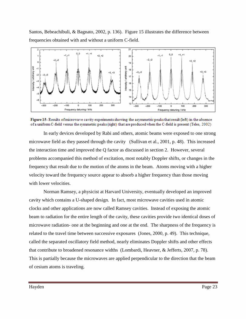
Asymmetrical frequency distributions can occur if the C-field is not uniform, which result in

additional measurement error when determining the resonance frequency (Teles, Magalhaes,

Hayden Page 23

Santos, Bebeachibuli, & Bagnato, 2002, p. 136). Figure 15 illustrates the difference between

frequencies obtained with and without a uniform C-field.

In early devices developed by Rabi and others, atomic beams were exposed to one strong

microwave field as they passed through the cavity (Sullivan et al., 2001, p. 48). This increased

the interaction time and improved the Q factor as discussed in section 2. However, several

problems accompanied this method of excitation, most notably Doppler shifts, or changes in the

frequency that result due to the motion of the atoms in the beam. Atoms moving with a higher

velocity toward the frequency source appear to absorb a higher frequency than those moving

with lower velocities.

Norman Ramsey, a physicist at Harvard University, eventually developed an improved

cavity which contains a U-shaped design. In fact, most microwave cavities used in atomic

clocks and other applications are now called Ramsey cavities. Instead of exposing the atomic

beam to radiation for the entire length of the cavity, these cavities provide two identical doses of

microwave radiation- one at the beginning and one at the end. The sharpness of the frequency is

related to the travel time between successive exposures (Jones, 2000, p. 49). This technique,

called the separated oscillatory field method, nearly eliminates Doppler shifts and other effects

that contribute to broadened resonance widths (Lombardi, Heavner, & Jefferts, 2007, p. 78).

This is partially because the microwaves are applied perpendicular to the direction that the beam

of cesium atoms is traveling.

Hayden Page 24

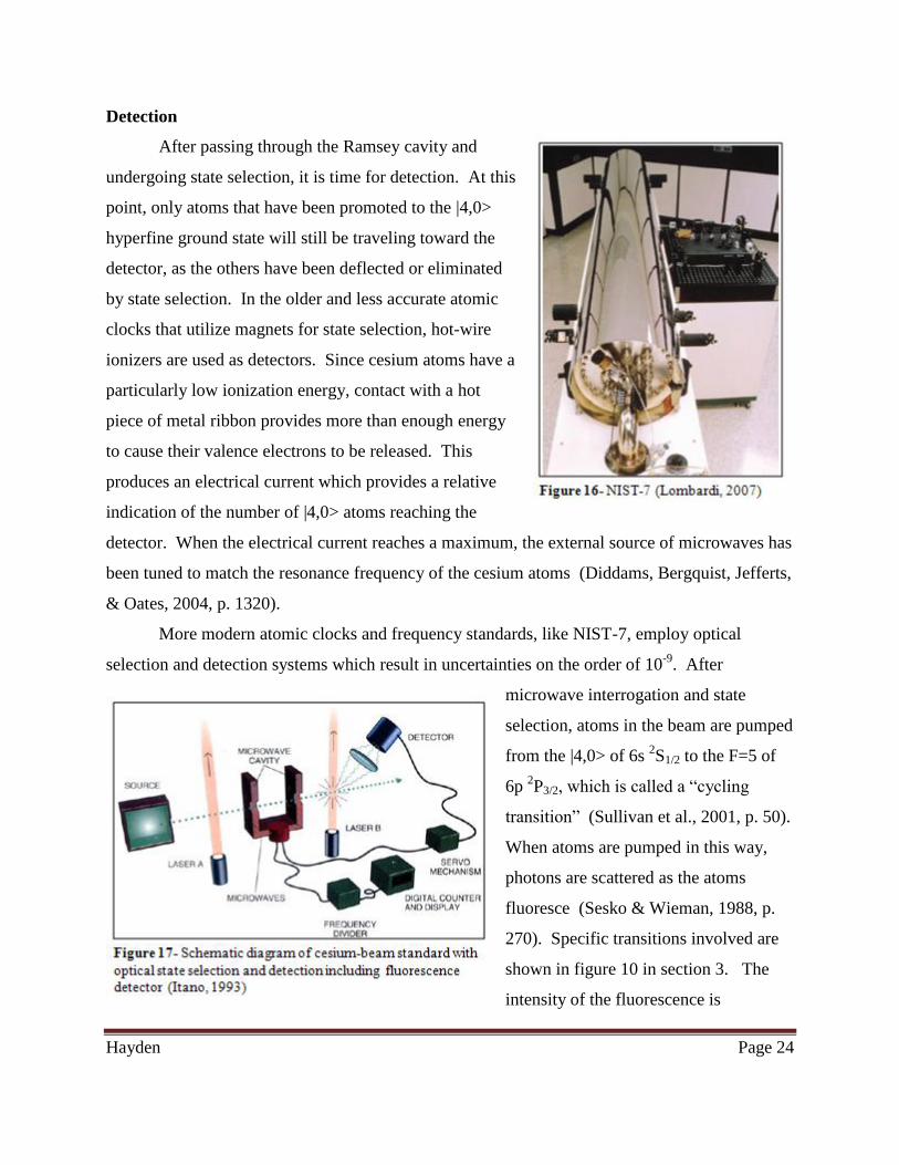
Detection

After passing through the Ramsey cavity and

undergoing state selection, it is time for detection. At this

point, only atoms that have been promoted to the |4,0>

hyperfine ground state will still be traveling toward the

detector, as the others have been deflected or eliminated

by state selection. In the older and less accurate atomic

clocks that utilize magnets for state selection, hot-wire

ionizers are used as detectors. Since cesium atoms have a

particularly low ionization energy, contact with a hot

piece of metal ribbon provides more than enough energy

to cause their valence electrons to be released. This

produces an electrical current which provides a relative

indication of the number of |4,0> atoms reaching the

detector. When the electrical current reaches a maximum, the external source of microwaves has

been tuned to match the resonance frequency of the cesium atoms (Diddams, Bergquist, Jefferts,

& Oates, 2004, p. 1320).

More modern atomic clocks and frequency standards, like NIST-7, employ optical

selection and detection systems which result in uncertainties on the order of 10-9

. After

microwave interrogation and state

selection, atoms in the beam are pumped

from the |4,0> of 6s 2S1/2 to the F=5 of

6p 2P3/2, which is called a “cycling

transition” (Sullivan et al., 2001, p. 50).

When atoms are pumped in this way,

photons are scattered as the atoms

fluoresce (Sesko & Wieman, 1988, p.

270). Specific transitions involved are

shown in figure 10 in section 3. The

intensity of the fluorescence is

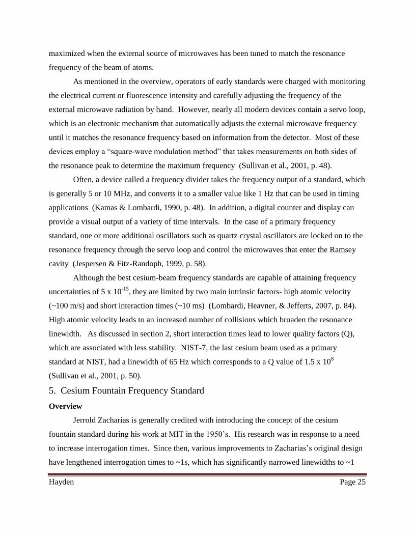
Hayden Page 25

maximized when the external source of microwaves has been tuned to match the resonance

frequency of the beam of atoms.

As mentioned in the overview, operators of early standards were charged with monitoring

the electrical current or fluorescence intensity and carefully adjusting the frequency of the

external microwave radiation by hand. However, nearly all modern devices contain a servo loop,

which is an electronic mechanism that automatically adjusts the external microwave frequency

until it matches the resonance frequency based on information from the detector. Most of these

devices employ a “square-wave modulation method” that takes measurements on both sides of

the resonance peak to determine the maximum frequency (Sullivan et al., 2001, p. 48).

Often, a device called a frequency divider takes the frequency output of a standard, which

is generally 5 or 10 MHz, and converts it to a smaller value like 1 Hz that can be used in timing

applications (Kamas & Lombardi, 1990, p. 48). In addition, a digital counter and display can

provide a visual output of a variety of time intervals. In the case of a primary frequency

standard, one or more additional oscillators such as quartz crystal oscillators are locked on to the

resonance frequency through the servo loop and control the microwaves that enter the Ramsey

cavity (Jespersen & Fitz-Randoph, 1999, p. 58).

Although the best cesium-beam frequency standards are capable of attaining frequency

uncertainties of 5 x 10-15

, they are limited by two main intrinsic factors- high atomic velocity

(~100 m/s) and short interaction times (~10 ms) (Lombardi, Heavner, & Jefferts, 2007, p. 84).

High atomic velocity leads to an increased number of collisions which broaden the resonance

linewidth. As discussed in section 2, short interaction times lead to lower quality factors (Q),

which are associated with less stability. NIST-7, the last cesium beam used as a primary

standard at NIST, had a linewidth of 65 Hz which corresponds to a Q value of 1.5 x 108

(Sullivan et al., 2001, p. 50).

5. Cesium Fountain Frequency Standard

Overview

Jerrold Zacharias is generally credited with introducing the concept of the cesium

fountain standard during his work at MIT in the 1950’s. His research was in response to a need

to increase interrogation times. Since then, various improvements to Zacharias’s original design

have lengthened interrogation times to ~1s, which has significantly narrowed linewidths to ~1

Hayden Page 26

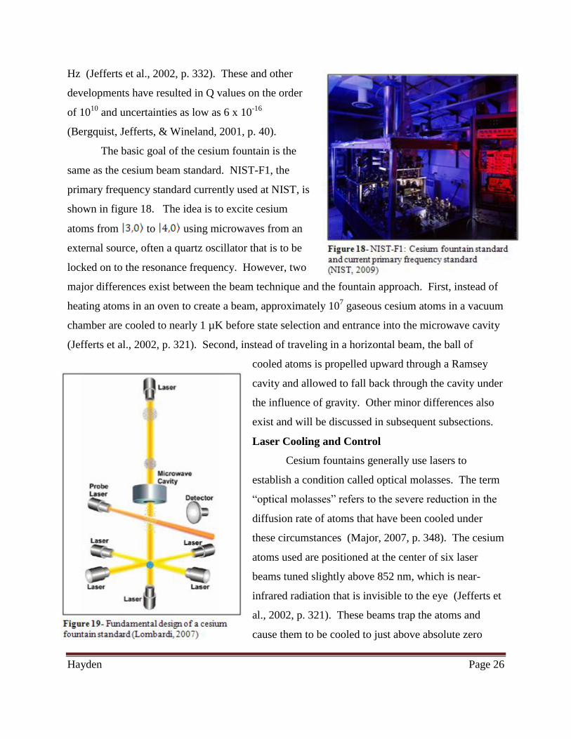
Hz (Jefferts et al., 2002, p. 332). These and other

developments have resulted in Q values on the order

of 1010

and uncertainties as low as 6 x 10-16

(Bergquist, Jefferts, & Wineland, 2001, p. 40).

The basic goal of the cesium fountain is the

same as the cesium beam standard. NIST-F1, the

primary frequency standard currently used at NIST, is

shown in figure 18. The idea is to excite cesium

atoms from to using microwaves from an

external source, often a quartz oscillator that is to be

locked on to the resonance frequency. However, two

major differences exist between the beam technique and the fountain approach. First, instead of

heating atoms in an oven to create a beam, approximately 107 gaseous cesium atoms in a vacuum

chamber are cooled to nearly 1 µK before state selection and entrance into the microwave cavity

(Jefferts et al., 2002, p. 321). Second, instead of traveling in a horizontal beam, the ball of

cooled atoms is propelled upward through a Ramsey

cavity and allowed to fall back through the cavity under

the influence of gravity. Other minor differences also

exist and will be discussed in subsequent subsections.

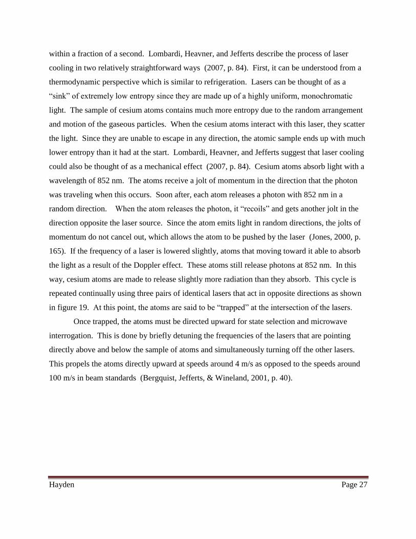
Laser Cooling and Control

Cesium fountains generally use lasers to

establish a condition called optical molasses. The term

“optical molasses” refers to the severe reduction in the

diffusion rate of atoms that have been cooled under

these circumstances (Major, 2007, p. 348). The cesium

atoms used are positioned at the center of six laser

beams tuned slightly above 852 nm, which is near-

infrared radiation that is invisible to the eye (Jefferts et

al., 2002, p. 321). These beams trap the atoms and

cause them to be cooled to just above absolute zero

Hayden Page 27

within a fraction of a second. Lombardi, Heavner, and Jefferts describe the process of laser

cooling in two relatively straightforward ways (2007, p. 84). First, it can be understood from a

thermodynamic perspective which is similar to refrigeration. Lasers can be thought of as a

“sink” of extremely low entropy since they are made up of a highly uniform, monochromatic

light. The sample of cesium atoms contains much more entropy due to the random arrangement

and motion of the gaseous particles. When the cesium atoms interact with this laser, they scatter

the light. Since they are unable to escape in any direction, the atomic sample ends up with much

lower entropy than it had at the start. Lombardi, Heavner, and Jefferts suggest that laser cooling

could also be thought of as a mechanical effect (2007, p. 84). Cesium atoms absorb light with a

wavelength of 852 nm. The atoms receive a jolt of momentum in the direction that the photon

was traveling when this occurs. Soon after, each atom releases a photon with 852 nm in a

random direction. When the atom releases the photon, it “recoils” and gets another jolt in the

direction opposite the laser source. Since the atom emits light in random directions, the jolts of

momentum do not cancel out, which allows the atom to be pushed by the laser (Jones, 2000, p.

165). If the frequency of a laser is lowered slightly, atoms that moving toward it able to absorb

the light as a result of the Doppler effect. These atoms still release photons at 852 nm. In this

way, cesium atoms are made to release slightly more radiation than they absorb. This cycle is

repeated continually using three pairs of identical lasers that act in opposite directions as shown

in figure 19. At this point, the atoms are said to be “trapped” at the intersection of the lasers.

Once trapped, the atoms must be directed upward for state selection and microwave

interrogation. This is done by briefly detuning the frequencies of the lasers that are pointing

directly above and below the sample of atoms and simultaneously turning off the other lasers.

This propels the atoms directly upward at speeds around 4 m/s as opposed to the speeds around

100 m/s in beam standards (Bergquist, Jefferts, & Wineland, 2001, p. 40).

Hayden Page 28

State Selection

State selection techniques used in fountain

standards differ from those utilized in beam standards,

because they involve both microwaves and optics.

Figure 20 shows a schematic diagram of the inside of

NIST-F1. After cooling and trapping, almost all

atoms occupy the 9 mf states of |4,0> (Sullivan et al.,

2001, p. 53). These atoms first travel through the

inactive detection region into a magnetically isolated

state selection cavity. This state selection cavity is

identical to the Ramsey cavity. It provides a short

burst of microwaves that drives as many atoms into

|3,0> as possible. Immediately after receiving this

dose of microwaves, a laser is used to remove any

additional |4,0> atoms using the same strategy

employed in beam standards. State selection in NIST-

F1 is able to remove greater than 99% of the |4,0>

atoms (Jefferts et al., 2002, p. 322).

Microwave Cavities

After state selection, the cesium atoms continue their ascent into the Ramsey cavity. The

structure and function of these cavities are the same as those used in the beam standards that

were previously explained. However, interaction time is lengthened as microwaves are applied

once on the way up and then again after the atoms reach the apogee and travel back down.

Detection

Once atoms have gone through the Ramsey cavity, optical techniques are used to

determine how many of the atoms made the desired |4,0> ↔ |3,0> hyperfine transition. As with

the beam standard, fluorescence detectors are used. In the case of the fountain standard, the

|3,0> atoms are also detected, as noise can be reduced by accounting for these atoms (Sullivan et

al., 2001, p. 54). In, NIST-F1, the |4,0> atoms are detected first by using a standing wave that

pumps atoms from F=4 to F=5 as shown in figure #. A mirror, an optical telescope, and a silicon

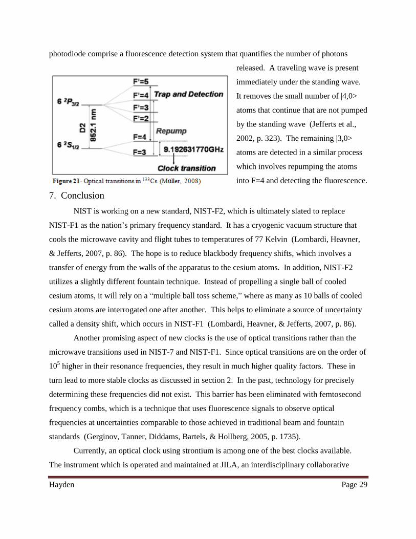
Hayden Page 29

photodiode comprise a fluorescence detection system that quantifies the number of photons

released. A traveling wave is present

immediately under the standing wave.

It removes the small number of |4,0>

atoms that continue that are not pumped

by the standing wave (Jefferts et al.,

2002, p. 323). The remaining |3,0>

atoms are detected in a similar process

which involves repumping the atoms

into F=4 and detecting the fluorescence.

7. Conclusion

NIST is working on a new standard, NIST-F2, which is ultimately slated to replace

NIST-F1 as the nation’s primary frequency standard. It has a cryogenic vacuum structure that

cools the microwave cavity and flight tubes to temperatures of 77 Kelvin (Lombardi, Heavner,

& Jefferts, 2007, p. 86). The hope is to reduce blackbody frequency shifts, which involves a

transfer of energy from the walls of the apparatus to the cesium atoms. In addition, NIST-F2

utilizes a slightly different fountain technique. Instead of propelling a single ball of cooled

cesium atoms, it will rely on a “multiple ball toss scheme,” where as many as 10 balls of cooled

cesium atoms are interrogated one after another. This helps to eliminate a source of uncertainty

called a density shift, which occurs in NIST-F1 (Lombardi, Heavner, & Jefferts, 2007, p. 86).

Another promising aspect of new clocks is the use of optical transitions rather than the

microwave transitions used in NIST-7 and NIST-F1. Since optical transitions are on the order of

105 higher in their resonance frequencies, they result in much higher quality factors. These in

turn lead to more stable clocks as discussed in section 2. In the past, technology for precisely

determining these frequencies did not exist. This barrier has been eliminated with femtosecond

frequency combs, which is a technique that uses fluorescence signals to observe optical

frequencies at uncertainties comparable to those achieved in traditional beam and fountain

standards (Gerginov, Tanner, Diddams, Bartels, & Hollberg, 2005, p. 1735).

Currently, an optical clock using strontium is among one of the best clocks available.

The instrument which is operated and maintained at JILA, an interdisciplinary collaborative

Hayden Page 30

project between NIST and the University of Colorado, is capable of operating at or below the

uncertainty level of 10-18

(Ludlow et al., 2008, p. 1806). It uses a lattice technique that traps

atoms before interrogation. This and other techniques such as Penning traps, magneto-optical

traps, and chip-scale atomic clocks are driving much of the current research.

In just under 100 years, uncertainty in time-related measurements has decreased by at

least 8 orders of magnitude. It is difficult to determine exactly how accurate the best clock is

today, since the progress seems to be occurring so quickly. In fact, many have compared

research in this area to hitting a moving target. Rapid progress in timekeeping, as a result of the

work of many renown contributors in multiple fields within physical science, is a perfect

example of advancements in science leading to dramatic lifestyle changes for ordinary people.

For this reason, the topic is exigent and relevant for everyone from experienced scientists to high

school learners.

Hayden Page 31

References

Arditi, M. (1982). A caesium beam atomic clock with laser optical pumping, as a potential frequency

standard. Metrologia, 18, 59-66.

Ball, D. W. (2007, January). Atomic clocks: An application of spectroscopy. Spectroscopy, 21(1).

Bergquist, J. C., Jefferts, S. R., & Wineland, D. J. (2001, March). Time measurement at the millennium.

Physics Today, 37-42.

Crowell, B. (2006). Bandwidth [Data file]. Retrieved July 24, 2009, from http://en.wikipedia.org/wiki/

File:Bandwidth2.png

Dennis, S. K. (2007). Cesium metal [Data file]. Retrieved July 15, 2009, from Wikipedia Web site:

http://upload.wikimedia.org/wikipedia/commons/2/2a/Csmetal.jpg.jpg

Diddams, S. A., Bergquist, J. C., Jefferts, S. R., & Oates, C. W. (2004, November 19). Standards of Time

and Frequency at the Outset of the 21st Century. Science, 306, 1318-1324.

Gerginov, V., Tanner, C. E., Diddams, S., Bartels, A., & Hollberg, L. (2004). Optical frequency

measurements of 6s 2S1/2–6p 2P3/2 transition in a 133Cs atomic beam using a. Physical Review

A, 70(042505), 1-8.

Gerginov, V., Tanner, C. E., Diddams, S. A., Bartels, A., & Hollberg, L. (2005). High-resolution

spectroscopy with a femtosecond laser frequency comb. Optics Letters, 30(13), 1734-1736.

Itano, W., & Ramsey, N. (1993, July). Accurate measurement of time. Scientific American, 56-65.

Jefferts, S. R., Shirley, J., Parker, T. E., Heavner, T. P., Meekhof, D. M., Nelson, C., et al. (2002).

Accuracy evaluation of NIST-F1. Metrologia, 32, 321-336.

Hayden Page 32

Jespersen, J., & Fitz-Randoph, J. (1999, March). From sundials to atomic clocks: Understanding time and

frequency (Monograph No. 155). Washington, DC: National Institute of Standards and

Technology.

Jones, T. (2000). Splitting the second. The history of atomic time. Bristol and Philadelphia: Institute of

Physics Publishing.

Kamas, G., & Lombardi, M. A. (1990, September). Time and frequency users manual. Washington: US

Government Printing Office.

Levine, J. (2002, July). Time and frequency distribution using satellites. Reports on progress in physics,

65, 1119-1164.

Lombardi, M. A., Heavner, T. P., & Jefferts, S. R. (2007, December). NIST primary frequency standards

and the realization of the SI second. The Journal of Mesurement Science, 2(4), 74-89.

Ludlow, A. D., Zelevinksy, T., Campbell, G. K., Blatt, S., Boyd, M. M., de Miranda, M. H. G., et al.

(2008, March 28). Sr lattice clock at 1 × 10−16 fractional uncertainty by remote optical

evaluation with a Ca clock. Science, 319, 1805-1808.

Major, F. G. (2007). The quantum beat: Principles and applications of atomic clocks (2nd ed.). New

York: Springer.

Markowitz, W., Hall, R. G., Essen, L., & Parry, J. (1958, August). Frequency of cesium in terms of

ephemeris time. Physical review letters, 1(3), 105-107.

Metcalf, H., & van der Staten, P. (1994, August). Cooling and trapping of neutral atoms. Physics Reports,

244(4), 203-386.

Hayden Page 33

Millman, S., & Zacharias, J. R. (1937). The signs of the nuclear magnetic moments of Li7, Rb85, Rb87,

and Cs133. Physical Review, 51, 1049-1052.

Müller, S. T., Magalhães, D. V., Bebeachibuli, A., Ortega, T. A., Ahmed, M., & Bagnato, V. S. (2008).

Free expanding cloud of cold atoms as an atomic standard: Ramsey fringes contrast. Journal of

the Optical Society of America B, 25(6), 909-914.

NASA. (2009). Voyager location in heliocentric coordinates. Retrieved from http://voyager.jpl.nasa.gov/

science/Vgrlocations.pdf

National Institute of Standards and Technology. (2009). Time and frequency from a to z: An illustrated

glossary. Retrieved June 28, 2009, from http://tf.nist.gov/general/glossary.htm

National Physical Laboratory. (2009). Essen’s Caesium Clock [Data file]. Retrieved from

http://www.npl.co.uk/upload//img_200/atomic_clock.jpg

Nave, C. R. (2006). Quantum physics. In Hyperphysics. Retrieved July 15, 2009, from Georgia State

University Department of Physics and Astronomy Web site: http://hyperphysics.phy-astr.gsu.edu/

hbase/quacon.html#quacon

NIST. (2009). Historical context of the SI. Retrieved August 7, 2009, from http://physics.nist.gov/cuu/

Units/history.html

NIST-F1 cesium fountain atomic clock [Physics laboratory: Time and frequency division]. (n.d.).

Retrieved July 20, 2009, from National Institute of Standards and Technology Web site:

http://tf.nist.gov/cesium/fountain.htm

NIST Physics Laboratory. (2001). Research highlights. Retrieved August 9, 2009, from

http://physics.nist.gov/Divisions/Div840/PLflyer/time.html

Hayden Page 34

NIST virtual museum. (2009). Retrieved July 24, 2009, from http://museum.nist.gov/realmuseum.html

Provechito, J. (2004). The very large array at at Socorro, New Mexico, United States. [Data file].

Retrieved from http://upload.wikimedia.org/wikipedia/commons/6/63/

USA.NM.VeryLargeArray.02.jpg

Ramsey, N. F. (1986). The successive oscillatory field method and the hydrogen maser. In 40th Annual

Symposium on Frequency Control.

Sesko, D. W., & Wieman, C. E. (1988). Observation of the cesium clock transtion in laser-cooled atoms.

Optics Letters, 14(5).

Sullivan, D. B., Bergquist, J. C., Bollinger, J. J., Drullinger, R. E., Itano, W. M., Jefferts, S. R., et al.

(2001). Primary atomic frequency standards at NIST. Journal of Research of the National

Institute of Standards and Technology, 106(1), 47-63.

Teles, F., Magalhaes, D. V., Santos, M. S., Bebeachibuli, A., & Bagnato, V. S. (2002). Characterization

of the brazilian Cs atomic-frequency standard: Evaluation of major shifts. Metrologia, 39, 135-

141.

Topp, M. Personal communication. July 16, 2009

Time services department [Leap seconds]. (2003). Retrieved July 24, 2009, from United States Navy Web

site: http://tycho.usno.navy.mil/time.html