1

Cereal Banking Impacts on Food and Nutrition Security and Resilience

building of rural households in The Gambia By Raymond Jatta 1

Abstract

Using Propensity score matching built on a stratification and randomisation, this paper

attempts to evaluate the impact of cereal banking on Food and Nutrition Insecurity. Cereal

Banking is a community-based risk management strategy which involves buying of food

during harvest when prices are low and storing for consumption during the lean period when

food prices are high. The purpose is to smooth consumption in rural communities and

households through the year.

The results of our matching indicate that communities that are relative poorer, living further

away from markets and are vulnerable to high inter-seasonal food price changes have a

higher probability of adopting and sustaining cereal banking schemes.

Our impact evaluation show that cereal banking has far reaching positive impacts on food

availability, accessibility and nutrition at individual, households and community level. In

particular, the results show an average treatment effect of 25 – 30% reduction in both the

food gap and inter-seasonal food price variability in treated villages. Cereal banking

enhances food self-sufficiency by an average of 11.6%. The Difference in mean between

children from households in treated villages and control villages show significant differences

of more than 16 percentage points between the average rates of malnutrition of children in

treated households and children from control villages. Like other studies, we observe that

the literacy of household head significantly improves the nutritional status of children.

Similarly, provision of farming implements has a significant impact on food and nutrition

security of rural households.

However, the impact on wealth seems to indicate that for cereal banking to enhance wealth

and other livelihood outcomes, it must be consistently operated for a while.

Introduction

Cereal banking is a community social safety net that is employed by communities in most

arid and semiarid regions of the world, especially in food deficit countries or regions (Bosu et

al 2012, Bhattamisha R 2012). It is defined as…..“as an organization in a village or group of

villages which buy, stores and sells food-grain in order to guarantee the food security of the

village community, and it is managed by a management committee appointed by this

community”…(Beer F 1990). The intuition behind cereal banks is that rural subsistent

agricultural households tend to sell the bulk of their farm produce at low prices at harvest but

during the lean period, they have to buy food (often the same products) at high prices. This

1 University of Cheikh Anta Diop, Dakar

2

inter-seasonal price variability tends to reduce income of farmers at harvest when they are net

sellers and erode their purchasing power during the lean period when they are net buyers.

Whilst storing food as a means of smoothing consumption is an age-long practice (Sampson,

2012, AITP 2012), the evidence show that the evolution and practice of cereal banking in

West Africa is closely linked with the drought that hit most of the region in the 1960s to the

1990s (SOS FAIM, 2009, Moussa 2010 p 3, Beer F 1990, CCAFS 2003). Recently, its

importance is being reemphasised as a policy initiative to manage the increasing recurrent

price and climate shocks negatively impacting on food and nutrition security of vulnerable

people and countries. For example, as part of its emergency response, the ECOWAS region

plans to operationalize more than 5000 cereal banking schemes in 12 member countries

(Rural Hub 2012).

Our review of the literature indicates that beside reports by promoters of cereal banking

(often aid organisations and NGOs), not much impact evaluation research has been conducted

about the usefulness of the practice. Evaluating its usefulness and viability will provide tools

on how to upscale, manage, redesign or upscale the scheme to build resilience to future

shocks.

Our focus is to test if cereal banking is useful in reducing food and nutrition insecurity and

enhance livelihood outcomes for participating households faced with the risk of price and

climate variability. We use a mix of randomisation, stratification and propensity score

matching to match treated and control villages and compare food and nutrition security

drivers and outcomes overtime.

Seasonality of Production and Consumption

Food production, affordability and consumption in most developing countries follow the

agricultural cycle (Bellemare and Barrett 2012). During harvest, food is in abundance and

most households become net supplier. In The Gambia, this period ranges from October –

February. Food supplies tend to move from rural areas following high demand and better

prices in the urban areas (Barrett C 1996). However, approaching the rainy season, food is

normally in short supply (FAO 2011, IFAD 2012). Rural households and communities

become net buyers and often have to rely on imported food from the urban areas. A flow

reversal of food occurs which is associated with higher prices in rural areas. Production

constraints exacerbated by the absence of large storage schemes and credit constraints tend to

worsen this spatial and temporal food availability and price changes (Barrett C, 1996). This

dynamics affect rural households and communities more, eroding incomes and causing

seasonal food and nutrition insecurity (CFSVA 2011). As a result food insecurity is much

more seasonal than it is a chronic problem in rural areas of The Gambia.

The main purposes of cereal banking are in three folds

1. Provide food to food deficit households during the lean period, which also coincides

with the farming period.

3

2. Preserve purchasing power of participating households due to high food prices during

lean periods by providing loans food (often on loan or at low prices) to participating

households

3. To act as first-to-reach emergency buffer stocks when disasters occur.

Context We conduct our research in three of the rural regions of The Gambia; Central River North,

Central Rive South and Upper River Regions. Beside their high poverty rates, malnutrition

and proportion of food insecure households, these regions are located further away from the

main export market, having relatively more adverse weather conditions and are home to more

than 85% of cereal banking initiatives in The Gambia (MICS 2006, CFSVA 2011). Poverty

rates in these regions are above the national average of 48% (IHS 2010). Price shocks and

frequent weather-induced crop failures are common covariate shocks that affect livelihood

and food security and are blamed for the countries inadequate progress in meeting its MDG1

(IFAD 2011, GoG MDGs Status Report 2007).

Like most other studies in The Gambia, the population distribution in the sample villages

show a youthful population of 75% being below 30 years old (IHS 2010, NPHS 2008).

Average household size is the sample communities is 12. The main economic activity is

farming with 80% of respondents above 12 years indicating that they are engaged in crop

farming, followed by livestock production and fishing respectively. The major crops

cultivated are millet, groundnut, rice and maize. There is also a gender dimension of cropping

system with men mainly cultivating upland crops; millet, maize and groundnut and women

concentrated in the cultivation of the main staple food; rice (Von Braun et al 1989, Carney

and Watts 2001).

The Gambia is characterised by arid and semi-arid zones with two seasons of about four

months of rainy season (June – September) and eight months of dry season (Ceesay M 2004).

Only less than 6% of arable land is irrigated (Von Braun et al 1989, Ceesay M 2004). In

addition to reducing rainfall trend, one of the most striking occurrence of climate change is

the increasing rainfall variability since the late 1960s exhibiting recurrent droughts and

changes in onset and cessation of rainfall and dry spell.(Camberlin and Diop, 2003, Ndaiye

and Batchiery 2005, Sima F 2010, CCAFS 2008). This is typical of the Sahel.

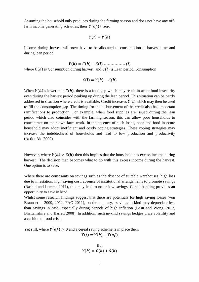
Agriculture is rainfed and as such production often varies with rainfall pattern (Rural Hub

2012). The figure below shows increasing variability of both rainfall and domestic food

production.

4

Source: Author

The Analytical Framework The practice of storage or food reserves is a precautionary savings mechanism which is

practiced to smooth consumption (Sarris et al 2006). Whilst the practice may be located

within the main theories of consumption and savings (Permanent Income Hypothesis and Life

Cycle Hypothesis), the major difference is the frequency of inter-temporal utility

maximisation objective. Communities in rural areas in arid countries employ savings as a risk

management strategy (Bhattamshira and Barrette 2008) with decisions not limited to Life

Cycles but more so frequent production, savings and consumption decisions across seasons of

an agricultural cycle from one harvest to the next (Deaton A 1998, Udry et al 2012). The

purpose is mainly to reduce the incidence of seasonal food insecurity and malnutrition.

It is commonly held as rational that consumers smooth consumption over their lifetime (see

see Deaton 2005 on Modigliani’s life cycle hypothesis). For agrarian households that produce

once in a year but have to consume for the whole of the year, smoothing consumption within

a single agricultural cycle is as important as the life cycle smoothing objective (Khandker,

2009, Basu and Wong 2012).

We can represent this in a simplified framework that allow us to show seasonal consumption

variability, credit and savings constraints

( ) ( ) ( )…………(1)

Where ( ) is Total Income, ( ) is Income at harvest and ( )) is Income off-farm

y = 0.123x - 1.3532 R² = 0.5549

y = 0.0685x - 0.753 R² = 0.1718

-2.5

-2

-1.5

-1

-0.5

0

0.5

1

1.5

2

2.5

3

0 5 10 15 20 25Var

iab

ility

Cereal Production and Rainfall Variability (1991

- 2012

Cereal Prod. Var

Rainfall Var.

5

Assuming the household only produces during the farming season and does not have any off-

farm income generating activities, then ( ) ≈ zero

( ) ( )

Income during harvest will now have to be allocated to consumption at harvest time and

during lean period

( ) ( ) ( ) ……………. (2)

where ( ) is Consumption during harvest and ( ) is Lean period Consumption

( ) ( ) ( )

When ( )is lower than ( ), there is a food gap which may result in acute food insecurity

even during the harvest period peaking up during the lean period. This situation can be partly

addressed in situation where credit is available. Credit increases ( ) which may then be used

to fill the consumption gap. The timing for the disbursement of the credit also has important

ramifications to production. For example, when food supplies are issued during the lean

period which also coincides with the farming season, this can allow poor households to

concentrate on their own farm work. In the absence of such loans, poor and food insecure

household may adopt inefficient and costly coping strategies. These coping strategies may

increase the indebtedness of households and lead to low production and productivity

(ActionAid 2009).

However, where ( ) ( ) then this implies that the household has excess income during

harvest. The decision then becomes what to do with this excess income during the harvest.

One option is to save.

Where there are constraints on savings such as the absence of suitable warehouses, high loss

due to infestation, high saving cost, absence of institutional arrangements to promote savings

(Rashid and Lemma 2011), this may lead to no or low savings. Cereal banking provides an

opportunity to save in kind.

Whilst some research findings suggest that there are potentials for high saving losses (von

Braun et al 2009, 2012, FAO 2011), on the contrary, savings in-kind may depreciate less

than savings in cash, especially during periods of high inflation (Basu and Wong, 2012,

Bhattamshire and Barrett 2008). In addition, such in-kind savings hedges price volatility and

a cushion to food crisis.

Yet still, where ( ) and a cereal saving scheme is in place then;

( ) ( ) ( )

But

( ) ( ) ( )

6

where ( ) is savings during harvest

( ) ( ) ( ) ( )……… (3)

Then ( ) ( ) ( ) ( ) ( )

( ) ( ) ( ) ………… (4)

This means that consumption during the lean period is financed by savings made at harvest

and income from off-farm income sources.

Relating ( ) ( ) ( ) and ⁄ , being inter-seasonal food prices changes. High

inter-seasonal food prices have the potential to reduce lean period consumption through

lessening real incomes and cash savings.

Thus if ( ) is in cash and where ⁄ is significantly high, then it may pay for savings to

be made in–kind than in cash. According to Von Braun at el 1989, AATG 2008, inter-

seasonal food price changes can be up to 300 – 400% which invariably suggests the gains in

physical food savings compared to savings in cash. The above is also true for off-farm

income that is used to purchase food. High food price inflation reduces Y(of).

In addition, savings can either be made at household level (private savings) or by a

community. The main difference between individual savings and community savings rests in

the rules and regulations on period of savings and credit distribution in the case of

community savings. In other words, whilst private stocks may be used anytime as the

household prefers disbursements in the case of collective savings is only allowed at critical

period of the hungry season (AATG 2009). In addition, cereal banking schemes tend to instil

a type of “forced savings in collective action” and thus encourage a high savings rate in a

community (Bhattmashira 2011). This notwithstanding, the risk of collective savings is

mismanagement by committee members and potential reduction in real value of stored

cereals due to poor storage when cereals are jointly stored (Beer F 1990, Kent 1989).

Methodology and Sampling Design Our methodology is based on a World Bank implemented Community Driven Development

Project (CDDP) in the Gambia 2008 - 2011. The project target rural communities across The

Gambia. Due to high village subscription and eligibility relative to fund availability, selection

of final beneficiary villages went through the following process (Arcand et al 2010).

1. Stratification

Using the National Population Census data of 2003 on village characteristics for more

than 930 villages in all seven of the eight regions of the Gambia2, a Poverty Index was

2 The number of regions are based on the Local Government Act of 2002

7

compiled for all the villages with a population of less than 10,000 inhabitants. The

Poverty Index comprised the following varaibles

i. Proportion of household heads who cannot read or write

ii. Proportion of households without electricity

iii. Proportion of households with clean drinking water

iv. Proportion of households without own toilet facilities

This stratification process was meant to set criteria for eligibility which eliminated

some villages. 950 out of more than 1800 villages were eligible

2. Randomisation

Out of the eligible villages, a randomisation was undertaken (by simple lottery) to

choose final set of 400 villages to be treated.

According to the Baseline report (Arcand et al 2010), a comparison of the characteristics of

the villages that were selected and those that did not from the randomisation produced fairly

similar average characteristics. As such evaluating such a project could employ Randomised

Control Trial. Of the 400 villages that received funding from CDDP about 12% chose to

implement cereal banking schemes from many possible subprojects based on community

members voting (Arcand et al 2010, Jaimovich D 2012).

Four years into the implementation of the CDDP project, we undertake to evaluate the impact

of cereal banking as a subproject on household food and nutrition security. Unlike, the

randomised CDDP treatment, the choice of cereal banking was endogenous to village

characteristics. The choice reflected the community members’ valuations of risks, aspirations

as well as the perceived benefits for which they expect cereal banking may address (Brooks

2009, Smit 2003). This risk could be that of food and nutrition insecurity caused by rainfall

and inter-seasonal price changes. We argue that these characteristics formed the determinants

to the choice of cereal banking and are most likely also going to influence the outcome. Thus,

any impact evaluation must have to control for these possible confounding factors in order to

eliminate selection bias (Angrist 2012, Baker, J. L., 2000, Rosenbaum and Robin 1983,

Heckman et al 1998).

This implied that

1. We had to have a set of useful village characteristics that determined choice of cereal

banking in other to answer the question, what are the determinants to the choice of

cereal banking.

2. Given these determinants, we can select control villages that had similar

characteristics with the treatment villages in terms of these determinants to choice of

cereal banking.

3. By implication, this will enable the two groups to be similar at baseline based on the

characteristics that determines the choice of cereal banking.

4. The assumption then is that given their similarities in these important observable

characteristics, impact of the programme on these two groups would be similar.

According to (Heckman and Ichimura 1997), the fulfilment of this assumption

produces a comparison group that resembles the treated group of an experiment in one

8

key respect: conditional on village characteristics X, the distribution of treatment

outcome Y0 given treatment D = 1 is the same as the distribution of control outcome

Y0 given non-treatment D = 0. This eliminates the problem of section bias. After

controlling for these confounding characteristics, the expected outcomes for the two

groups is similar to being random (Duflo and Kramer 2003).

E(Y0 | X;D = 1) = E(Y0 | X;D = 0) … ie similar baseline averages

5. Thus if one is given treatment and another used as a control (not given treatment) then

difference in these two groups after treatment will be an unbiased estimator of the

treatment effect.

The option was to used quasi experiments and in particular Propensity Score Matching

(PSM) (Heckman and Ichimura 1997, Baker, J. L., 2000, Duflo and Saez 2002 Duflo and

Kramer 2003). This was also necessary given data limitations.

Technically, PSM rely on the conditional independence assumption. If we can ascertain that

the characteristics that compel communities or households receiving treatment or choosing a

project are independent of the outcomes of interest, we can reasonably attribute changes. This

assumption is called the unconfoundedness assumption, or conditional independence

assumption (Rosenbaum and Rubin 1983):

(YTi, Y

Ci)Ti|Xi

This is to say that if it can be reasonably ascertained that selection into treatment (Ti = 1)

given the observable covariates (Xi) is uncorrelated or independent to the outcomes of

interest; YT and Y

C, we can assume validity of the unconfoundedness assumption.

Determinants to Choice of Cereal Banking

Bottom-up participatory approach to development is increasingly being championed as an

effective way to improved project performance and targeting for service delivery (Wong S

2012, Mansuri and Rao 2004). Despite the potentials to be affected by elite capture and free

rider behaviours (Olken B 2012), it is increasing being applied in project delivery. This was

the case of the CDDP (Arcand et al 2010). It is important to note that funding was allocated

to the treatment villages but the choice of what community project to implement was left for

community members to choose. An important question to ask therefore was; what determines

the choice of one subproject in a community and another in another community, in particular

cereal banking?

Several researches on such decision making posit that local information on risk, vulnerability,

social capital factors coupled with the expected benefits of an intervention determine choice

of an intervention (Brooks 2009). There is a likelihood that when presented with two options,

a consumer will chose the option that is expected to yield the maximum benefits (Ravallion

2010). This intuition can also be applied to a group of individuals or a community. When

faced with the option to choose from an array of possible interventions, the community will

9

choose the intervention which is expected to give the highest return. This is at the heart of

economic thinking.

For example, (Smit 2003 and Brooks 2009) posit that the choice of an adaptation or risk

management strategy is based on

1. A community valuation of risk occurrence and its possible impacts

2. The importance the community attaches on the adaptation or risk management

strategy.

Cereal banking is a community risk management strategy and a social safety net that reduces

the risk of food insecurity caused by rainfall variability and food price variability. Our choice

of variables included factors such as price and rainfall variability, drivers and proxies of

poverty and food insecurity, biophysical and demographic characteristics etc.

We use data on 27 pre-treatment village socioeconomic, climate, livelihood assets and

demographic characteristics to construct our propensity score. In addition, we collect data on

livelihood assets such as physical and natural assets/resources available for each village or

area. These also include geographical location of a village with respect to main roads, forest

resources and other important resources. Data on rainfall variability and price volatility are

obtained from meteorological stations whilst data on prices of cereals were obtained at local

markets nearest to each of the villages used in our PSM.

Mathematically, our model is expressed as;

( ) ( ) ( ) ( )

Where P(CB) is the probability of participating in a cereal bank, β represent parameter that

must be estimated, Vc is a vector of pre-exposure control village level characteristics ;

social, economic, livelihood, natural and market characteristics and ε is the error term of all

factors that are not controlled for in our model.

In the case of the study, it was useful to generate control villages to each of the treated village

so that a unique pair is mapped. One-to-One nearest neighbour matching algorithm without

replacement (Caliendo and Kopeinig 2005, p.9) was applied for this study. An individual

from the comparison group is chosen as a match for a treated individual based on the

predicted probability to choose cereal banking (Sianesi B. 2010).

The Propensity Scores

Due to its binary nature, PSM is carried out using either a probit or logit model (Caliendo and

Kopeinig 2005) as indicated in equation (1). Our PSM on both treated to partial control and

pure control produced fairly similar results. We interpret the P-Values and the signs of the

coefficients3

3 The Coefficients are not marginal effects but on odd ratios.

10

Partial Control PSM Pure Control PSM

Variable Coefficient P>|z| Coefficient P>|z|

Coeff of Variation (Rainfall) 13.8706 0.286 16.076 0.246

Coeff of Variation ()rice) 660.3531 0.006** 681.091 0.018*

Poverty 7.2494 0.035* 2.695 0.041*

Fruit Trees 0.0512 0.033* 0.043 0.102

Millet grown 0.00134 0.004** 0.000** 0.009**

Crop farmers 46.2541 0.029* 32.713 0.053

Average HH size 0.7248 0.209 0.283 0.501

No daily mkt 0.1836 0.046* 0.152 0.058

No improved trans 0.5373 0.009** 0.476 0.038*

Dominant ethnicity gr. 3 14.6823 0.003** 7.953 0.009**

Dominant ethnicity gr. 2 7.4451 0.004** 3.842 0.113

Connect & lowland Villages 1.1066 0.109 1.618 0.039*

Distance to market 0.5274 0.038* 0.446 0.033*

Proximity of the LGA 33.20208 0.024* 33.592 0.02**

Proximity of the District 2.873271 0.021* -3.023 0.016*

Cov_Price2 1128.559 0.004** -1157.499 0.016**

N. of 0bservations 451 422

R2 0.4549 0.3947

P<0.05*, P<0.01**

Our PSM results show the variables that are important determinants to choice of cereal

banking. The price risk shown by the covariance of price calculated by the standard deviation

over the mean prices of main food crops positively affects choice of cereal banking.

Proximity to markets, poverty rates, cropping systems and infrastructure are also significant

determinants to choice of cereal banking. These results are similar to (Bhattamishra 2012).

Villages that are relatively poorer, remote and poorly integrated in markets, having fewer

infrastructures and suffer from rainfall and price volatility are more likely to choose and

sustain cereal banking schemes.

The results of the PSM point to the fact that self-assessment of risk and vulnerability of

events to livelihood outcomes drives choices of adaptation or risk management strategy (Smit

2003). Targeting on the basis of need and likelihood for survival is important for cereal

banking and safety nets in general.

11

To test the robustness of out propensity score matching and setting a solid foundation for the

impact evaluation, we test our PSM. The test show that the matched treated and control

villages have similar propensity scores and that there is no significant difference between the

treated and control villages before cereal banking.

Variable Sample Treated Partial Control T-stat

Coefficient of Variation ( price) Unmatched 0.2647 0.2428 2.92

Matched 0.2644 0.2625 0.19

Poverty Index Unmatched 0.7061 0.6543 2.7

Matched 0.7061 0.732 -1.23

Millet per cap Unmatched 227.289 148.82 2.15

Matched 227.289 221.77 0.08

HHs with Fruit trees Unmatched 4332.19 5795.61 -1.61

Matched 4332.19 3811.68 0.76

Crop farmers Unmatched 0.9657 0.921 4.14

Matched 0.96574 0.9681 -0.41

Av. HH Size Unmatched 11.419 11.12 0.62

Matched 11.419 11.64 -0.33

No daily market Unmatched 81.476 62.65 4.24

Matched 81.47 82.54 -0.27

Distance from market Unmatched 43.308 41.83 0.55

Matched 43.3 45.168 -0.77

No Improved transport Unmatched 98.22 91.72 3.43

Matched 98.229 97.668 0.54

Remote & Upland Villages Unmatched 0.5106 0.4108 1.31

Matched 0.5106 0.5106 0.00

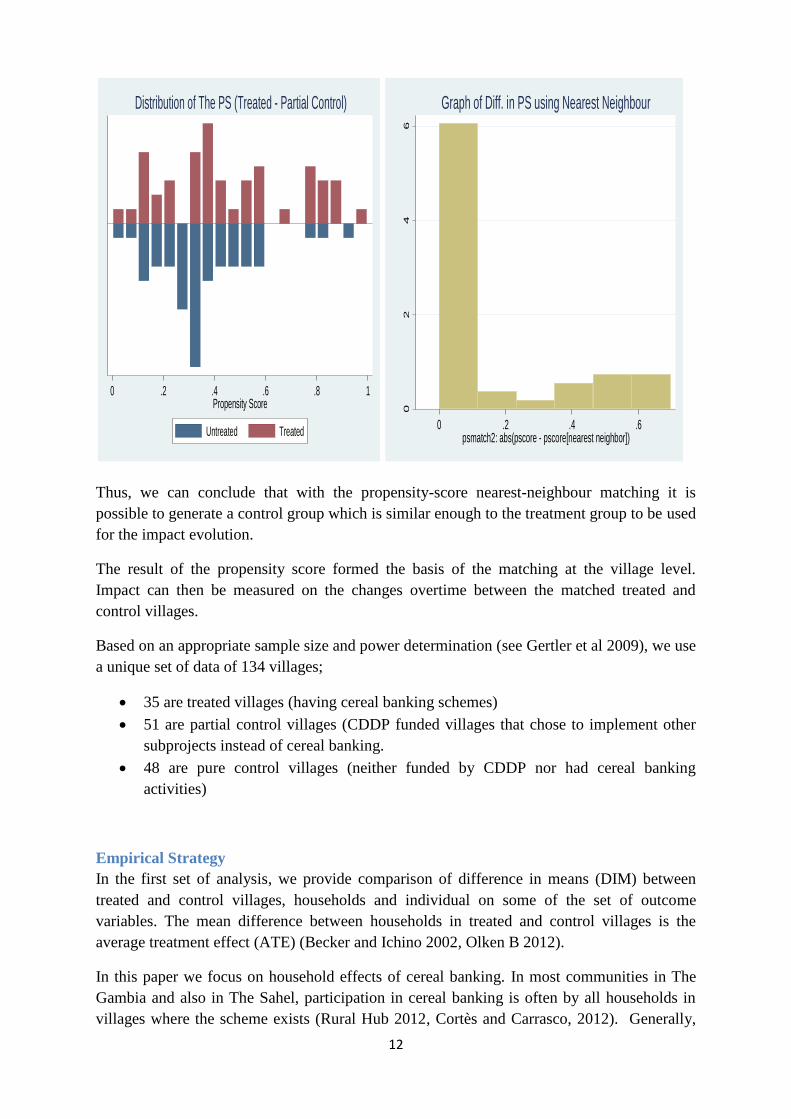
In addition, the graph indicates the possibility of a common support and that the distribution

of the difference in the matched treated and control villages shows that more 70% of the

difference is between 0 – 0.1.

PSM Results

Treated and Pure Control

Treated and Partial Control

Variable Obs Mean Min Max Obs Mean Min Max

Propensity score 422 0.1836 0.0000 0.9842 451 0.1042 0.0000 0.9614

Diff in matched neighbours 47 0.1464 0.0001 0.5198 47 0.1514 0.0001 0.496

12

Thus, we can conclude that with the propensity-score nearest-neighbour matching it is

possible to generate a control group which is similar enough to the treatment group to be used

for the impact evolution.

The result of the propensity score formed the basis of the matching at the village level.

Impact can then be measured on the changes overtime between the matched treated and

control villages.

Based on an appropriate sample size and power determination (see Gertler et al 2009), we use

a unique set of data of 134 villages;

35 are treated villages (having cereal banking schemes)

51 are partial control villages (CDDP funded villages that chose to implement other

subprojects instead of cereal banking.

48 are pure control villages (neither funded by CDDP nor had cereal banking

activities)

Empirical Strategy

In the first set of analysis, we provide comparison of difference in means (DIM) between

treated and control villages, households and individual on some of the set of outcome

variables. The mean difference between households in treated and control villages is the

average treatment effect (ATE) (Becker and Ichino 2002, Olken B 2012).

In this paper we focus on household effects of cereal banking. In most communities in The

Gambia and also in The Sahel, participation in cereal banking is often by all households in

villages where the scheme exists (Rural Hub 2012, Cortès and Carrasco, 2012). Generally,

0 .2 .4 .6 .8 1Propensity Score

Untreated Treated

Distribution of The PS (Treated - Partial Control)

02

46

Den

sity

0 .2 .4 .6psmatch2: abs(pscore - pscore[nearest neighbor])

Graph of Diff. in PS using Nearest Neighbour

13

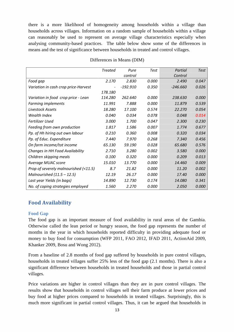
there is a more likelihood of homogeneity among households within a village than

households across villages. Information on a random sample of households within a village

can reasonably be used to represent on average village characteristics especially when

analysing community-based practices. The table below show some of the differences in

means and the test of significance between households in treated and control villages.

Differences in Means (DIM)

Treated Pure control

Test Partial Control

Test

Food gap 2.170 2.830 0.000 2.490 0.047

Variation in cash crop price-Harvest -178.180

-192.910 0.350 -246.660 0.026

Variation in food crop price - Lean 114.280 262.640 0.000 238.630 0.000

Farming implements 11.991 7.888 0.000 11.879 0.539

Livestock Assets 18.280 17.100 0.574 22.270 0.054

Wealth Index 0.040 0.034 0.078 0.048 0.014

Fertilizer Used 3.000 1.700 0.047 2.300 0.230

Feeding from own production 1.817 1.586 0.007 1.774 0.677

Pp. of Hh hiring out own labour 0.210 0.360 0.008 0.320 0.034

Pp. of Educ. Expenditure 7.440 7.970 0.268 7.340 0.456

On farm income/tot income 65.130 59.190 0.028 65.680 0.576

Changes in HH Food Availability 2.710 3.280 0.002 3.580 0.000

Children skipping meals 0.100 0.320 0.000 0.209 0.013

Average MUAC score 15.010 13.770 0.000 14.460 0.009

Prop of severely malnourished (<11.5) 8.7 21.82 0.000 11.20 0.002

Malnourished (11.5 – 12.5) 12.19 26.17 0.000 17.40 0.000

Last year Yields (in bags) 14.890 12.730 0.174 14.080 0.341

No. of coping strategies employed 1.560 2.270 0.000 2.050 0.000

Food Availability

Food Gap

The food gap is an important measure of food availability in rural areas of the Gambia.

Otherwise called the lean period or hungry season, the food gap represents the number of

months in the year in which households reported difficulty in providing adequate food or

money to buy food for consumption (WFP 2011, FAO 2012, IFAD 2011, ActionAid 2009,

Khanker 2009, Bosu and Wong 2012).

From a baseline of 2.8 months of food gap suffered by households in pure control villages,

households in treated villages suffer 25% less of the food gap (2.1 months). There is also a

significant difference between households in treated households and those in partial control

villages.

Price variations are higher in control villages than they are in pure control villages. The

results show that households in control villages sell their farm produce at lower prices and

buy food at higher prices compared to households in treated villages. Surprisingly, this is

much more significant in partial control villages. Thus, it can be argued that households in

14

control villages suffer more from season price fluctuations which can inhibit their access to

food and increase income poverty. .

Yields and Investments

Researcher argue that increasing own-production is one of the most effective ways of

reducing hunger in rural communities. For example, Ramirez conclude that a 1% increase in

yields is associated with a 0.12% increase in the Human Development Index (Ramírez R,

2002 p7). The results shows that average crop yield in 2012 were better in treated households

than control households. The difference may be explained given that when food is available

or is secured, households can afford to invest more in inputs such as fertilizer. The above is in

line with the risk aversion literature which postulates that the higher the income smoothing

options, the higher the willingness to invest in riskier (less risk averse) but higher return

investments (Yesuf and Bluffstone 2007, Karlan D 2012, Cole et al 2012, Modruch 2009,

Heltberg R 2008).

Similarly, several studies suggest that yields of crops and profitability of farming activities

respond positive to fertilizer application (Xu Z 2006, Akponikpe P 2008). Our results show

that whilst households that participate in cereal banking reported purchasing and applying 3

bags of inorganic fertilizer in the last cropping season, households in partial and pure control

villages apply only 2.3 and 1.7 bags of fertilizer respectively. This represents a difference of

30 – 40% fertilizer application. It must be noted that a bag of fertilizer costs as much as a bag

of rice and may be worth as much as 4 weeks of feeding for an average 12 member

household.

Ability to store food as in cereal banking reduce time spent in search for food during periods

of scarcity at the expense of concentrating on own production (ActionAid 2009, OXFAM

2013). Coupled with adoption of inefficient coping strategies such as taking loans at high

interest, giving out own labour for payment, investments in inputs influences the ability of

households to produce enough food to meet their consumption. Such investments enhance the

timely completion of farming activities, production and yields. Evidently, households in

treated villages are able to produce more food to feed their households for a longer period of

the year than households in control villages4.

Table 1: Months of Feeding from Own Production

4 Feeding from own production is a categorical variable (1 being producing less than 5 months and 4 being

producing food enough for more than 12 months of household food needs)

15

Vividly, whilst only 55.01% of households in control villages claim to be able to produce

more than half of their food needs from their own production, as much as 62.09% of

households in treated villages produce more than half of their food needs in a year.

Stability

Changes in Food Availability – (From Harvest to Lean)

Several studies are on a consensus that in the Gambia, during the lean period, both the

quantity and quality of food for most rural households reduces significantly (CFSVA2011,

IFAD 2011, FAO 2012). This however varies for different households given their

accumulated livelihood assets/endowments and also access to credit schemes such as cereal

banking. From the analysis, it is observed that a significantly larger proportion of households

in control villages reported significant reduction in both food quantity and quality of food in

control villages than in treated villages. Reduction in food quantity and quality from harvest

to the lean period shows the extent of seasonal food insecurity among rural households in the

Gambia (Bosu and Wong 2012, Khander 2009, CFSVA 2011).

Food Accessibility From the data, it can be shown that about 75% of household expenditure is on food. Income

spent on Health and Education accounts for about 11% and 7.5% of household expenditure

respectively. Research suggests that poor households spend a higher percentage of their

income on food and less on other livelihood needs (FAO 2011, Wright and Cafiero 2012).

This is linked to the theory of marginal propensity to consumption and savings (Deaton A

1989). This implies that among such food deficit households, any increase in food prices

affect them the most as they spend relatively a higher percentage of their income on food

(Kalkuhl M et al 2013). In addition, it is also argued that once the ability of meeting

household food demands are threatened, other needs suffer first (AATG 2008). Unlike food

availability indicators, cereal banking does not have as much impact on income sources

37.91

42.48

18.61

1

44.09 44.09

11.02

0.79

0

5

10

15

20

25

30

35

40

45

50

< 5 months 5 - 8 months 8 - 12 months > 12 months

% of Treated HHs % of Control HHs

16

diversification and expenditure. We observe that households which participate in cereal

banking tend to use most of their income on food and have less diversified income sources.

Although these differences are not significant, they tend to explain the level of vulnerability

to rainfall dependent livelihood activities (Warner, K. et al 2013 p1).

Wealth Index

The wealth index which sums up livestock, housing, farming implements and domestic assets

is higher in partial control villages than in both treated and pure control villages though the

difference is not statistically significant. The above indicators are used as proxy for wealth oi

food security assessments (Morris S 1999, Doocy and Burnham 2009, Saaka and Osman

2013, CFSVA 2011). This suggests that cereal banking has little impact or that the significant

impact of cereal banking on wealth may only be realised after implementing the scheme for a

while. This is uncommon for such community-based interventions. In rural communities

where the constraint is on safety or suitable private storage infrastructure relative to the risk

of fires, theft or borrowing from other, the presence of cereal banking schemes provide a

security against the risks. From the graph, it can be observed that treated households have

slightly a higher proportion of households having corrugated and cement buildings than

control villages.

Nutrition

Anthropometric Analysis

The Mid Upper Arm Circumference (MUAC) is one of the anthropometric measures of food

and nutrition security but in particular, level of malnourishment among children. The recently

published WHO guideline 2013 reported that the anthropometric assessments methods of

weight-to height and MUAC were good and consistent methods for measuring wasting

(WHO 2013). It is applied to children under five years as they are observed to respond more

quickly to short term changes in food intake and quality (Pangaribowo E et al 2013).

The WHO guideline of 1995 revised in 2013 suggest that in children who are aged 6 – 59

months, severe malnutrition be defined as

1. Weight-for-height of ≤-3 Z score or

2. MUAC of < 11.5cm

3. Presence of bilateral oedema

Whilst weight–to-height measure may be more appropriate for measuring age specific

differences, MUAC is simpler and has a superior correlation to risk of death (WHO 2013,

p25). It is also cheaper to use especially in measuring short term and emergency phenomena

than other measures of malnutrition. According to Myatt et al, 2006, MUAC is less prone to

mistakes and interviewers influence when compared to weight for child measure of

malnutrition. Despite the absence of generally agreeable standard or cut off points, most

researchers adopt the 1995 WHO recommended cut off points (Biswas S et al 2013).

17

MUAC Reading Colour Description

Below 11.5 cm Red Severe acute malnutrition

11.5 – 12.5 Red Moderate acute malnutrition

12.5 – 13.5 Yellow Risk of malnutrition

Above 13.5 Green Well nourished

Source: WHO 1995

We use a dataset of 980 children aged between 1 – 5 years old from the sampled households.

The average MUAC reading for the children in our sampled villages is 14.0cm which using

the WHO 1995 recommended cut off points indicate that on average 65% of children in the

sample areas are well nourished or that 35% of the children in our sample suffer from

moderate to acute levels of malnutrition (MICS 2010, Mwangome Martha et al 2012). This

is slightly above the national average of 22% in 2006 (MICS 2006). It would have been

interesting to measure MUAC of children in different periods of the year (lean and post-

harvest) to assess the impact of these seasonal food security differences.

Comparing children from households in treated villages to their counterparts in control

villages, we observe that households in treated villages have higher MUAC averages and are

thus better nourished. The results show that on average a higher percentage of children and

adults skip meals in control villages than in treated villages which may adversely affect

energy and micronutrient intake adequacy (Rolls B et al, 2002, 2010). This is reflected from

the MUAC readings and the proportion of children who are severely malnourished, showing

significant differences between households in treated, pure and partial control villages

respectively. We also observe a higher deviation from the median MUAC reading for

children in control households than their counterparts in treated households.

51

01

52

05

10

15

20

Pure Control Partial Control

Treated

mu

ac r

ea

din

g

Graphs by Participation in cereal banking and CDDP_Vill

Midupper Arm Circumference for Children (Treated and Control)

18

The results show that 8.7% of children in treated households are severely malnourished

whilst 11.2% and 21.82% are severely malnourished in households from partial and pure

control villages respectively. It is often observed that children respond quickly to even short

term changes in food intake and as such these differences may be attributed to food

availability, skipping of meals and intake differences across households in treated and control

villages during the critical lean period (Pangaribowo E et al 2013)

It has recently been questioned whether MUAC is age- and sex dependent (NC Roy 2011,

WHO 2013). After reviewing the scientific evidence underlying the use and interpretation of

MUAC, a WHO Expert Committee established in the 1990s to review and report on

assessment, monitoring and evaluation of FNS indicators recommended for an age and

gender sensitive MUAC measure (Onis M et al 1997 WHO and UNICEF 2009).

We therefore compare MUAC readings among treated and control villages categorised

according to their ages. Using the same 11.5cm cut of point; we observe that MUAC is age

sensitive as fewer children suffer malnutrition the higher their ages; level of malnutrition

reducing from 18.8% in less than two-year old to less than 1% among five-year old children

This results supports earlier research findings supporting the need to adjust the MUAC cut-

off point to respond to age as undertaken in some studies (Myatt M, 2006). However, we

observe a slightly lower level of malnutrition in less than one year olds than 2-years old.

Similar results in Mahgoub, Nnyepi and Bandeke 2006, were attributed to care giving

(breastfeeding) being more in younger ages reducing the occurrence of underweight among

children during breastfeeding. We found this argument plausible for our case though we do

not have data to prove this claim.

In addition to the MUAC for age categorisation, we also undertake a MUAC for sex

comparison. Unlike (Choudhury K et al 2000) who found a significant MUAC gender gap in

Bangladesh, our MUAC - gender interactions results were not dissimilar among male and

female under-five year old children.

Coping Strategies Rural agricultural households have often learnt to adapt with exogenous changes that threaten

their livelihoods (Boko M et al 2007) such as price and rainfall risk. These coping strategies

are short term means of hedging the impact of a risk factor. The impact of price and rainfall

variability which can range from increasing poverty, hunger or mortality can either be mild,

medium or high. This will depend among other things on;

1. The probability of severity of the shock (hazard)

2. The degree to which livelihoods are dependent on the shock (exposure)

3. Household access or stock of these livelihood assets and coping strategies (Maxwell

D 1995 IPCC, 2007).

19

Coping with Risks to Food and Nutrition Insecurity

Mild Medium High (Risk)

Changing Cropping Systems When both the probability of the occurrence of shocks and its potential impact are high

(resulting in high risks) households often adopt more coping strategies than when probability

and potential impact are mild (Maxwel et al 2000). However, the use of these coping

strategies has different implications on livelihood stability in the short and long term.

When rainfall and price variability is experience or is expected, households in The Gambia

often adopt other cropping systems to hedge the impact (Ceesay M 2004). These include

adopting high yielding or early maturing crop varieties, changing from cash crop to food crop

production etc. These strategies are implemented before a hazard occurs and in the literature

considered to be adaptation strategies.

Borrowing Another option that is often adopted to reduce impact once a shock occurs includes

borrowing. On average 70% of respondents interviewed highlighted that they take loans from

middlemen and moneylenders whilst 30% secure loans from family members and friends in

the village. Whilst networks, exchange of land, credit, labour etc are a strong pillar of rural

Gambian society (Jamiovich 2012, Yilma et al 2014), during the lean period, most other

households are affected by food insecurity. This is because price volatility is also a covariate

risk which is incurred by all (Gilbert C 2012) in a given locality. Thus during the lean period,

rural networks of exchange slightly become less effective, at least for food loans within a

cluster of villages. However, this reduces the larger the area of analysis. Depending on the

location of the village relative to lowland food surplus producing areas, poor harvest upland

is often mitigated by borrowing from households in the lowland areas close to the fresh water

source of the River Gambia (von Braun et al 1989, Carney and Watts 2001).

Hired

labour Distress sale

of livestock &

other assets

Changes in

cropping

system

Taking

Loans

Migration Reduced food

intake

(frequency,

quality and

quantity

Coping strategies used

20

Distress Sale of Livestock

Livestock is often kept as savings (buffer stock) which can be used during periods of need

especially in rural communities with little or no financial market penetration (Fafchamps M

et al 1996). Extreme events such as drought can lead to distress sale of livestock (Kaitibie,

Moyo and Perry 2008) during which time livestock is sold at low prices or in exchange for

some quantity of cereals. Our data show that there is evidence of distress selling of livestock,

as most sales occurred between July to September also corresponding to the hungry season

(FAO 2011).

Hiring out own labour The lean period in The Gambia also coincides with the farming season. In the absence of

food during this period, most households will offer their own labour to work in other farmers

farms in exchange for food, credit or money to buy food. This tends to disengage farmers

from their own production leading to vicious cycles of indebtedness, low production and

poverty (Bazin F 2004). Evidently, households in treated communities engage less in hiring

out their labour in exchange for food or payments for food during the critical lean period than

households in control villages.

Food Related Coping Strategies Other coping strategies employed in rural areas against threats to household security include

the use of less preferred foods, borrowing food from friends and kinsmen, reduce number and

frequency of meals, restricting consumption by adults or temporary migration (Deressa -

2010, Yilma et al 2014). From our data, households tend to use less preferred food, reducing

meal sizes and borrowing than other coping strategies. Using less preferred food, reducing

meal sizes or frequency of meals have a more direct an immediate impact on food and

nutrition security in the very short run (Ivanic et al. 2011, Hoddinott et al 2008).

Since some of the variables are categorical varaibles, we conduct both ttest and the Wilcoxon

rank-sum test to test for significance in the differences in our outcome indicators between

treated and control villages. Often the Wilcoxon rank-sum (Mann-Whitney) test is used in

place of the ttest in testing for differences in means or proportions for categorical and binary

varaibles. It is widely used in experimental and quasi experiments (Sawilowsky S 2005). We

present both the results to assess how robust the tests are for categorical and continuous

outcome indicators.

Estimating Treatment Effect on the Treated

Cross sectional analysis Given the successful matching, a cross-sectional econometric regression analysis using

Ordinary Least Square Estimation (Olken B 2012) can then be implemented, controlling for

village - and household level characteristics to estimate the actual impact of cereal banking

on treated households. In other words, we attempt to quantitatively estimate the influence of

cereal banking on the outcome of interest on the treated. This is similar to estimating the

Average Treatment Effect on the Treated (ATET) or the Intention to Treat (ITT) (Arcand et

al 2009, Duflo, Glennerster and Kremer 2007).

21

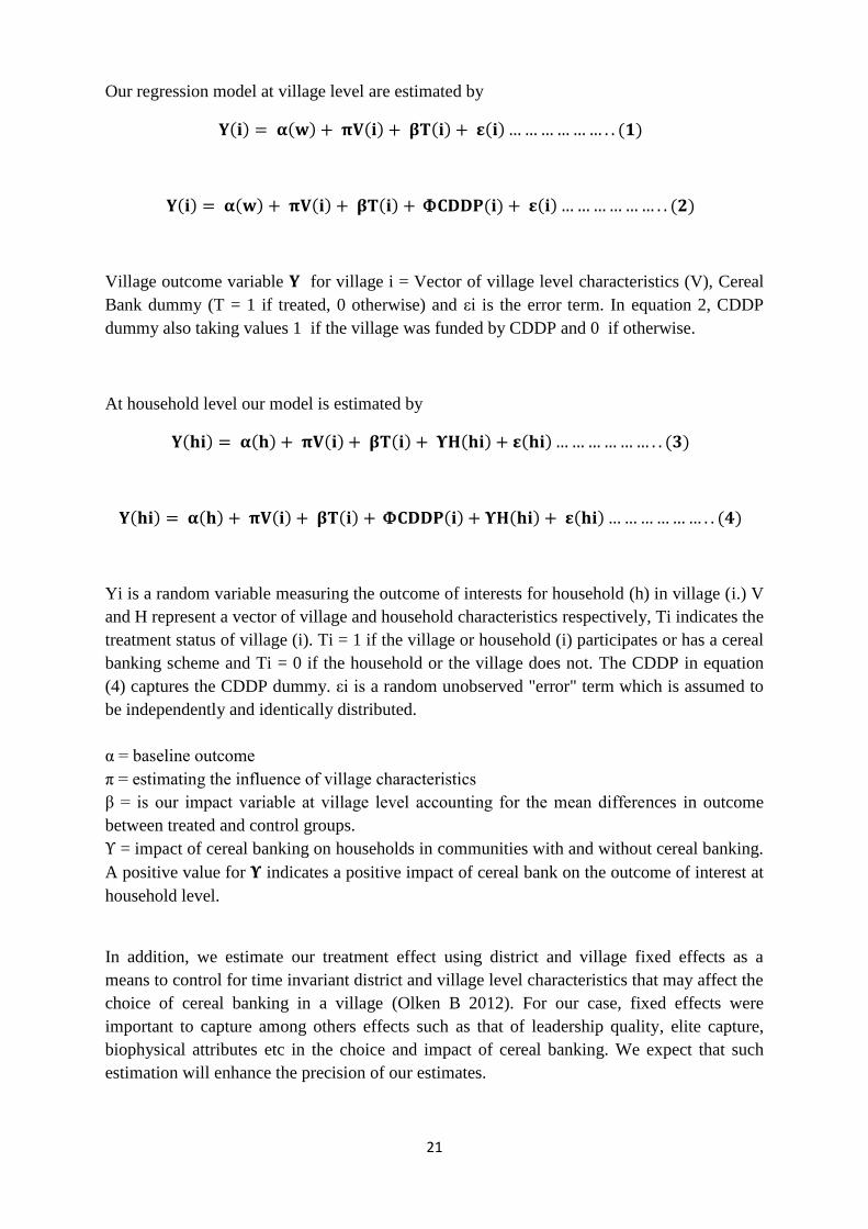
Our regression model at village level are estimated by

( ) ( ) ( ) ( ) ( ) ( )

( ) ( ) ( ) ( ) ( ) ( ) ( )

Village outcome variable for village i = Vector of village level characteristics (V), Cereal

Bank dummy (T = 1 if treated, 0 otherwise) and εi is the error term. In equation 2, CDDP

dummy also taking values 1 if the village was funded by CDDP and 0 if otherwise.

At household level our model is estimated by

( ) ( ) ( ) ( ) ( ) ( ) ( )

( ) ( ) ( ) ( ) ( ) ( ) ( ) ( )

Yi is a random variable measuring the outcome of interests for household (h) in village (i.) V

and H represent a vector of village and household characteristics respectively, Ti indicates the

treatment status of village (i). Ti = 1 if the village or household (i) participates or has a cereal

banking scheme and Ti = 0 if the household or the village does not. The CDDP in equation

(4) captures the CDDP dummy. εi is a random unobserved "error" term which is assumed to

be independently and identically distributed.

α = baseline outcome

π = estimating the influence of village characteristics

β = is our impact variable at village level accounting for the mean differences in outcome

between treated and control groups.

= impact of cereal banking on households in communities with and without cereal banking.

A positive value for indicates a positive impact of cereal bank on the outcome of interest at

household level.

In addition, we estimate our treatment effect using district and village fixed effects as a

means to control for time invariant district and village level characteristics that may affect the

choice of cereal banking in a village (Olken B 2012). For our case, fixed effects were

important to capture among others effects such as that of leadership quality, elite capture,

biophysical attributes etc in the choice and impact of cereal banking. We expect that such

estimation will enhance the precision of our estimates.

22

Food availability

Food self-sufficiency is an important driver to food security especially in rural communities

in developing countries (Deb Uttam et al 2009). This is even more so in the face of recurrent

global food crisis which makes reliance on own food production for consumption more

appropriate. The regression results show the treatment effect of cereal banking on food self-

sufficiency measured by the number of months households depend on their own farm and off

farm production or income to meet food needs of the households.

(1) (2) (3) (4) (5)

VARIABLES Self-Sufficiency

Treatment Dummy

Self-Sufficiency

CDDP Dummy

Self-Sufficiency

District FE

Self-Sufficiency

Pure Cont plus FE

Self-Sufficiency

Part Cont plus FE

Treatment 0.182** 0.0883 0.160** 0.168* 0.141

(0.0704) (0.0786) (0.0800) (0.0961) (0.0853)

Hired Labour -0.0303 -0.0384 -0.0750 0.00871 0.0592

(0.0711) (0.0707) (0.0742) (0.101) (0.0948)

Food Expenses -0.00597* -0.00486 0.00158 0.00337 0.00159

(0.00336) (0.00337) (0.00359) (0.00495) (0.00424)

Education expenses -0.00771 -0.00675 -0.00173 0.00190 -0.00477

(0.00506) (0.00504) (0.00520) (0.00715) (0.00608)

PP. of Self-produced 0.00739*** 0.00672*** 0.00541** 0.00542* 0.00255

(0.00218) (0.00218) (0.00224) (0.00279) (0.00281)

Age of HH head 0.00435* 0.00417* 0.00320 0.00243 0.00178

(0.00235) (0.00233) (0.00229) (0.00302) (0.00285)

No. of HH members 0.0184 0.0225 0.0224 0.00408 0.0294*

(0.0144) (0.0144) (0.0140) (0.0179) (0.0174)

No. of Farmer -0.0239** -0.0241** -0.0218* -0.00712 -0.0115

(0.0119) (0.0118) (0.0125) (0.0163) (0.0161)

Farming Implement 0.0596** 0.0525** 0.0860*** 0.0588* 0.0644**

(0.0244) (0.0244) (0.0259) (0.0325) (0.0299)

CDDP Village 0.218*** 0.0401

(0.0838) (0.0862)

District Dummy 4 0.710*** 0.710*** 0.791**

(0.196) (0.267) (0.372)

District Dummy 9 0.841*** 0.965*** 0.869**

(0.228) (0.272) (0.377)

Observations 459 459 459 294 327

R-squared 0.281 0.295 0.389 0.450 0.390

The treatment effect of cereal banking on food self-sufficiency is positive and significant

implying that cereal banking enhances food self-sufficiency by an average of 11.6%. When

the CDDP dummy is introduced in model (2), the results also show a positive and significant

impact of CDDP on food self-sufficiency. However, this renders the impact of cereal banking

insignificant. We also observe negative influence of coping strategies, food and education

expenditure on food self-sufficiency whilst revenue sources being from own production

positively influences self-sufficiency.

The key policy implications are that cereal banking and improving access to farming

implements are important for enhancing the capacity of smallholders to be food self-

sufficient. However, unlike as though, the numbers of household members who are farmers

23

tend to reduce the ability of households to be food self-sufficient. This may imply that other

income sources are more productive than farming or that diversified income sources for

households have a better influence on food production.

We also estimate the ATET using village level fixed effects. Similar to Olken B 2012, this

was incorporate to reduce bias that may result from unobservable but time invariant village

characteristics confounding the results of our estimation. More importantly, the result show a

positive and significant impact of irrigation enable double cropping on food self-sufficiency.

District 4 and 9 are rice growing areas that have access to Tidal Irrigation Infrastructure

(Ceesay M 2004, Carney et al 1992). The estimation with fixed effects produces similar

results to that without fixed effects. However, the higher R2

depicts higher precision for the

model with fixed effects. However, with or with fixed effects, the average treatment effect on

the treated is positive.

Our results show positive and significant impact of cereal banking on fertilizer application,

improving fertilizer application by at least 12.8%.

Contrary to earlier literature, the proportion of land borrowed by households significantly

improves fertilizer application. For example, it is argue that land ownership enhances

investment in long term productivity enhancement inputs which may improve yields, food

production and self-sufficiency (Feinerman and Peerlings 2002, Deininger and Jin 2006,

Hagos H 2012). This may be explained by the fact that most borrowed lands are marginal

lands in upland areas that require fertilizer application (ActionAid 2012). Similarly, double

cropping which is carried out in lowland areas during the dry season requires fertilizer

(1) (2) (3) (4) (5)

VARIABLES Fertilizer use

Treatment Dummy

Quantity fertilizer

CDDP Dummy

Fertilizer Use

District Fix. Eff.

Fertilizer

Pure Cont plus FE

Quantity fertilizer

Part Cont plus FE

Treatment 0.354** 0.282 0.307* 0.461** 0.128

(0.163) (0.180) (0.174) (0.225) (0.229)

Land_Borrowed 0.123** 0.123* 0.132** 0.179* 0.151*

(0.0625) (0.0625) (0.0668) (0.0924) (0.0855)

Double_cropping 0.380 0.400 0.0422 0.302 -0.886*

(0.283) (0.284) (0.314) (0.420) (0.517)

Feeding_Ownproduction -0.175 -0.191* -0.0760 -0.0201 -0.144

(0.107) (0.108) (0.113) (0.134) (0.145)

Food_Expenses -0.00125 -0.000510 -0.00707 -0.00260 -0.00679

(0.00749) (0.00753) (0.00836) (0.0108) (0.0108)

No_Coping_Strategies 0.0568 0.0634 0.0719 -0.0257 0.199*

(0.0699) (0.0702) (0.0767) (0.106) (0.108)

NNotliterate -0.0829*** -0.0856*** -0.0862*** -0.0746** -0.122***

(0.0280) (0.0281) (0.0294) (0.0376) (0.0379)

Farmer -0.305 -0.308 -0.187 -0.310 -0.358

(0.207) (0.207) (0.222) (0.279) (0.288)

WealthIndex 4.612*** 4.646*** 4.443*** 1.785 8.456***

(0.904) (0.904) (0.916) (1.095) (1.432)

District Dummy 9 -0.558 -0.786 -0.980

(0.485) (0.533) (0.908)

cddp_vill 0.180

(0.187)

Observations 452 452 452 289 322

R-squared 0.329 0.330 0.355 0.360 0.449

Standard errors in parentheses *** p<0.01, ** p<0.05, * p<0.1

24

application to maintain soil fertility (Jaimovich and Jatta 2014 forthcoming). The proportion

of food expenses, household head being farmer and illiterate negatively impacts on fertilizer

application. This may be due to the investment cost and information required for fertilizer

application. The CDDP dummy shows a positive impact on fertilizer application. The use of

fixed effects enhances our precession as it increases our R2 and standard errors.

The important policy implication is that beside affordability, education of farmers though

extension services significantly improves investments and technology adoption.

Food Stability Variables (1) (2) (3) (4) (5)

Food_Quantity in Food Qty

Treatment Dummy

in Food Qty

CDDP Dummy

in Food Qty

District Fixed Eff

in Food Qty Part

Cont plus FE

in Food Qty

Pure Cont plus FE

Treatment -1.160*** -1.320*** -1.142*** -0.542* -1.388***

(0.201) (0.220) (0.215) (0.279) (0.255)

Feeding_Ownproduction -0.272** -0.309** -0.201 -0.0761 -0.106

(0.127) (0.130) (0.139) (0.171) (0.164)

Hired_Labour 0.845*** 0.824*** 1.401*** 0.940*** 1.435***

(0.183) (0.184) (0.213) (0.273) (0.266)

Fertilizer_applied -0.296 -0.296 -0.678*** -1.168*** -0.370

(0.239) (0.239) (0.258) (0.330) (0.309)

age -0.0211*** -0.0213*** -0.0173** -0.0232*** -0.0210**

(0.00656) (0.00656) (0.00672) (0.00872) (0.00828)

N 0.0329 0.0345 0.000726 -0.0141 0.00112

(0.0347) (0.0347) (0.0357) (0.0429) (0.0403)

NFrom30to65 -0.0766 -0.0791 -0.0162 0.0226 -0.00246

(0.0835) (0.0838) (0.0856) (0.111) (0.0991)

Notliterate 0.870*** 0.929*** 0.257 0.478 0.270

(0.210) (0.213) (0.238) (0.302) (0.303)

WealthIndex 0.741 0.893 0.492 0.698 0.438

(1.024) (1.032) (1.072) (1.329) (1.572)

District Dummy 4 -1.491** -1.491* -1.172

(0.631) (0.850) (1.025)

District Dummy 9 -1.866*** -1.611** -1.837*

(0.599) (0.657) (0.973)

Cddp_vill -0.421*

(0.224)

Observations 452 452 452 289 322

R2 0.0748 0.0773 0.1135 0.1352 0.1283

Standard errors in parentheses ** p<0.01, ** p<0.05, * p<0.1

Using an Ordered Logit, we estimate the effect of cereal banking on the stability of the

quantity of food used for household consumption from harvest to lean period. Changes in

food quantity is self-reported categorical variable in which 1 indicates more stability whilst 5

indicates less stability. Our results show a negative treatment effect of cereal banking on food

quantity instability. This implies that cereal banking significantly reduces household food

instability. This is also true for access to double cropping and food self-sufficiency showing

the positive influence of irrigation which is possible for district 4 and 9. On the other hand,

households that practice hiring out own labour and large household sizes tend to increase

food instability. This is also true of age of household head and the proportion of household

members within active working age of 30-65 years.

25

The result clearly point to the fact that households that are poor are likely to adopt less

efficient coping strategies such as hiring out their own labour are more vulnerable and suffer

from seasonal food insecurity.

The treatment effect on the level of nutrition measured by the Midupper Arm Circumference

score is positive and significant whilst land borrowing has a negative effect on nutrition of

children. The number and frequency by which households employ food related coping

strategies has a negative impact on the level of nutrition. Polygamy and illiteracy of

household head negative impacts on nutrition level,

In agreement with recent literature and empirical findings, nutritional level of children as

measured by an unadjusted MUAC cut-off mark of 11.5cm indicate that the malnutrition

reduces with age of children. This supports the argument for an MUAC-Age comparison.

Unlike our age-MUAC interaction, we do not observe any significant difference between

male and female children in in their MUAC scores although females tend to have a lesser

MUAC scores than male children as shown by the regression results.

Like other studies, we observe that the literacy of household head significantly improves the

nutritional status children.

(1) (2) (3) (4) (5)

MUAC Score

Treatment Dummy

MUAC Score

CDDP Dummy

MUAC Score

District FE

MUAC Score

Pure Cont plus FE

MUAC Score Part

Cont plus FE

Treatment 0.668 0.488 0.710 1.032 0.491

(0.215)** (0.237)* (0.219)** (0.315)** (0.217)*

% of land borrowed -0.178 -0.181 -0.149 -0.108 -0.211

(0.081)* (0.081)* (0.085) (0.116) (0.087)*

Fertilizer (inorganic) 0.325 0.352 0.184 0.292 0.625

(0.270) (0.269) (0.271) (0.335) (0.284)*

Children skipping meals -0.704 -0.797 -0.653 -0.967 -0.833

(0.259)** (0.264)** (0.266)* (0.351)** (0.330)*

Marital status 0.055 0.060 0.146 0.186 0.071

(0.155) (0.154) (0.151) (0.188) (0.155)

No. of Coping Strategies -0.253 -0.253 -0.178 -0.240 -0.080

(0.090)** (0.090)** (0.097) (0.135) (0.109)

Age categories of children 0.561 0.547 0.534 0.495 0.465

(0.066)** (0.067)** (0.068)** (0.091)** (0.071)**

Gender of Child -1.040 -1.041 -1.100 -1.745 -1.311

(0.300) (0.302) (0.275) (0.085) (0.075)

HH head Not literate -0.748 -0.726 -0.688 -1.086 0.029

(0.207)** (0.207)** (0.255)** (0.321)** (0.293)

CDDP_Vill 0.451

(0.252)

District Dummy 4 1.427 1.868 0.913

(0.609)* (0.826)* (1.068)

District Dummy 9 0.357 0.169 1.685

(0.574) (0.646) (1.057)

Observations 366 366 366 239 261

R-squared 0.47 0.48 0.55 0.59 0.60

Standard errors in parentheses * significant at 5%; ** significant at 1%

26

Conclusion

According to the (FAO 2013), the majority of the World’s 842 million hungry are rural

smallholders or landless people in developing countries without access to productive

resources, especially Sub Saharan Africa. The Gambia, like most West Africa has

experienced very little progress in reducing food insecurity and child malnutrition in the past

20 years (Lopriore and Ellen 2003, ECA 2012, IFPRI 2012) and is off track in meeting

MDG1 (GoG 2009). This is due to a composite of factors such as recurrent climate shocks

compounded by low level of human development and import dependence. Food markets have

been proved to be inherently volatile (Kalkuhl M et al 2013) and a total dependence on these

markets exposes economies to shocks and uncertainties in their food and nutrition security.

Having responsive safety nets is thus critical to the attainment and stability of food and

nutrition security of the teeming poor population in food deficit importing countries.

We attempted to evaluate the impact of cereal banking by comparing food and nutrition

security outcomes between households that practice the schemes and similar counterfactual

households without the schemes. Our results vividly supports our hypotheses that cereal

banking is important for enhancing food and nutrition security at community, households and

individual levels and in all the four dimensions; food availability, accessibility and nutrition

and stability. The strongest effects are found in indicators of food availability, stability and

nutrition. The least effects are on wealth proxies.

In the rural areas of the Gambia, as in many other rural areas of developing countries, food

self-sufficiency is an important food and nutrition security driver. In terms of food intake,

the mere fact that food is supplied to households at critical period of the lean period reduces

the food gap, smooth consumption and stabilizes food intake. This has a bearing on avoiding

malnutrition, hunger. This also helps households to avoid the long term consequences of

short term food insecurity situations even for under-five-year old children.

The evidence of lower prices and lesser price variability in communities that operate cereal

banking schemes also support our hypothesis that cereal banking affect food accessibility by

reducing inter-seasonal food price variability by an average of 25%.

Our regression results showing the average treatment effect on the treated (ATET) implies

that participation in cereal banking reduces changes in food availability from harvest to lean

periods and thus enhances smooth consumption for participating households. The treatment

effect of cereal banking on food self-sufficiency is positive and significant implying that

cereal banking enhances food self-sufficiency by an average of 11.6%. Households who

participate in cereal banking reported stability in the quantity of food they consume during

the lean period, and this can be attributed 40% to the impact of cereal banking. This is partly

explained by the fact that cereal banking provides physical food credit facilities which are

meant to ensure that the quantity of food available remain stable throughout the year (Sarris

et al 2006). The treatment effect on the yields of participating households is quiet significant.

Yields on average increases by 12 bags of cereals and reduces the number of days households

had offered to hire out their own labour for food by 14 days or 11.7%. Participation in cereal

banking enable household invest in their farming operations more in terms of their time,

27

equipment and inputs. Our results show positive and significant impact of cereal banking on

fertilizer application, improving fertilizer application by at least 12.8%. The investments

enhance yields and on average build the capacity to feed from own production.

Contrary to what we hypothesised, there is a positive but insignificant impact of cereal

banking on wealth score. Our wealth score combines the score for household ownership of

domestic assets, farming implements, access to electricity, toilet facilities and the nature of

housing materials used. The positive coefficient on the treatment indicates a positive

treatment effect, implying that participation in cereal banking activities enhances wealth.

Conversely, it is also observed that the treatment effect on the number of coping strategies is

significant different from zero implying that participation in cereal banking reduces the

number of coping strategies a household employs.

Participation in cereal banking enhances the nutritional level of children in participating

households by 1.5 MUAC scores. The DIM show significant differences of more than 16

percentage points between the rates of malnutrition of children in treated households and

children from control villages. Like other studies, we observe that the literacy of household

head significantly improves the nutritional status children.

Beside the treatment effect of cereal banking, we observe that education of rural household

heads is important for enhancing the nutrition of children as well as adoption of technology

such as fertilizer application. Similarly, provision of farming implements has a significant

impact on food self-sufficiency or rural households

References

ActionAid the Gambia, 2008, Territorial Development Initiative (TDI), Agrarian diagnosis and

stakeholder analysis of Niamina East district.

Arcand J et al 2010, The Gambia CDDP baseline: rural household survey, qualitative survey, village

network survey.

Baker, J. L., 2000, Evaluating the Impact of Development Projects on Poverty: A Handbook for

Practitioners

Basu and Wong 2012, Evaluating Seasonal Food Security Programs in East Indonesia

Barrett R 2012, Grain Bank Survival and Longevity: Evidence from Orissa

Bhattamishra and Barrett 2010, Community-Based Risk Management Arrangements: A Review ,

World Development Vol. 38, No. 7, pp. 923–932, 2010

Caliendo and Kopeinig 2005 Some Practical Guidance for the Implementation of Propensity Score

Matching IZA DISCUSSION PAPER SERIES DP No. 1588

Ceesay M 2004, Management of Rice Production Systems to increase productivity in The Gambia,

West Africa, Cornell University

Cortès and Carrasco, 2012, Oxfam GB, Oxfam GB, Oxfam House, ISBN 978-1-78077-204-2

28

Daviron and Douillet 2013, Major players of the international food trade and the world food security

FOODSECURE Working paper no. 12

Duflo, Glennerster and Kremer 2007, Using Randomization in Development Economics Research: A

Toolkit* CEPR Discussion Paper No. 6059

Fafchamps M et al 1996, Drought and Saving in West Africa: Are Livestock a Buffer Stock?

Department of Economics, North western University.

FAO 2011, The State of Food Insecurity in the World, How does international

Government of The Gambia, March 2007, Poverty Analysis of The Gambia, Household Poverty

Survey, 2003 – 2004, Banjul

Institute for Agriculture and Trade Policy 2012 Grain Reserves and the Food Price Crisis: Selected

Writings from 2008–2012,

Heckman and Ichimura 1997, Characterising Selection Bias using experimental data

Kalkuhl, Kornher, Marta Kozicka, Pierre Boulanger, Maximo Torero 2013 Conceptual framework on

price volatility and its impact on food and nutrition security, FOODSECURE Working paper no. 15

Kent 1998, Community-level Grain Storage Projects (Cereal Banks) Why do they Rarely Work and

What are the Alternatives

Luers A. 2005, The surface of vulnerability: An analytical framework for examining environmental

change

Maxwell D 1995, Measuring Food Insecurity: The frequency and Severity of "Coping Strategies"

IFPRI FCND Discussion Paper no. 8

Mendelsohn R 2010, Efficient adaptation to Climate Change Yale School of Forestry and

Environmental Studies

Morris S et al 1999, Validity of rapid estimates of Household Wealth and Income for Health surveys

in Rural Africa FCND DISCUSSION PAPER NO. 72

Pangaribowo, Gerber and Torero 2013 Food and Nutrition Security Indicators: A Review

FOODSECURE working paper 05

Ravallion M 2000, Evaluating Anti-Poverty Programs Development Research Group, World Bank

Susan Wong 2012, What Have Been the Impacts of World Bank Community-Driven Development

Programs? CDD Impact Evaluation Review and Operational and Research Implications

Tadesse, Algieri, Kalkuhl and von Braun 2013, Drivers and triggers of international food price spikes

and volatility

von Braun 2011, Food price volatility and FNS, Center for Development Research, University of

Bonn

von Braun and Maximo Torero, 2009, Implementing Physical and Virtual Food Reserves to Protect

the Poor and Prevent Market Failure, International Food Policy Research Institute

29

von Braun and Tadesse, Global Food Price Volatility and Spikes: An Overview of Costs, Causes, and

Solutions, ZEF- Discussion Papers on Development Policy No. 161, Center for Development

Research, Bonn, January 2012, pp. 42.ISSN: 1436-9931

Wright and Cafiero 2009, Grain Reserves and Food Security in MENA Countries, University of

California, Berkeley

Annexes

0.2

.4.6

.80

.2.4

.6.8

Pure Control Partial Cont

Treated

Cheap/less pref. food Borrowing Food

Reducing Meal Sizes Reduce Adult Consup

Reduce Freq of meals No. of Strat. used

Graphs by Participation in cereal banking and CDDP_Vill

Food Related Coping Strategies

(1) (2) (3) (4) (5)

No. of Coping

Strategies Treatment

Dummy

No. of Coping

Strategies CDDP

Dummy

No. of Coping

Strategies District

Fixed Effects

No. of Coping

Strategies Pure

Cont plus FE

No. of Coping

Strategies Part Cont

plus FE

Treatment -0.516 -0.502 -0.529 -0.780 -0.387

(0.115)** (0.127)** (0.110)** (0.129)** (0.125)**

% of land borrowed 0.075 0.075 0.101 0.011 0.112

(0.044) (0.044) (0.043)* (0.055) (0.048)*

Fertilizer (inorganic) -0.371 -0.372 -0.134 -0.139 -0.091

(0.143)** (0.143)** (0.137) (0.157) (0.154)

Self labour hired 0.373 0.376 0.010 0.241 -0.206

(0.112)** (0.112)** (0.116) (0.135) (0.138)

Notliterate 0.268 0.265 0.305 0.121 0.337

(0.112)* (0.113)* (0.124)* (0.144) (0.150)*

Livestock Val -0.004 -0.004 -0.015 -0.012 -0.018

(0.007) (0.007) (0.007)* (0.007) (0.009)*

Food quantity -0.121 -0.119 -0.033 -0.002 0.013

(0.042)** (0.043)** (0.041) (0.046) (0.048)

CDDP_Vill -0.036

(0.131)

District Dummy 4 -1.427 -2.097 -1.151

(0.296)** (0.371)** (0.492)*

30

District Dummy 9 -1.716 -1.355 -1.928

(0.313)** (0.319)** (0.516)**

Observations 452 452 452 289 322

R-squared 0.37 0.37 0.52 0.59 0.54

Standard errors in parentheses * significant at 5%; ** significant at 1%