centre for research on globalisation and labour …

Centre for Research on Globalisation and Labour Markets, School of Economics,University of Nottingham

The Centre acknowledges financial support from The Leverhulme Trust underProgramme Grant F114/BF

CENTRE FOR RESEARCH ON GLOBALISATION AND LABOUR MARKETS

Research Paper 2000/19

Multinational Enterprises and NewTrade Theory: Evidence for the

Convergence Hypothesis

by

Salvador Barrios, Holger Görg and Eric Strobl

The Authors

Salvador Barrios is Research Fellow in the School of Economic Studies, University of

Manchester, Holger Görg is Research Fellow in the School of Economics, University of

Nottingham and Eric Strobl is Lecturer in Economics, University College Dublin.

Acknowledgements

The authors are grateful to David Greenaway, participants of the ETSG 2000 conference in

Glasgow, the CEPR workshop on “Labour Market Effects of Foreign Direct Investments” in

Madrid, and a GLM workshop in Nottingham for helpful comments on an earlier draft. All

remaining errors are, of course, their own. This research has benefited from financial support

through the “Evolving Macroeconomy” programme of the Economic and Social Research

Council (Grant No. L138251002), the European Commission Fifth Framework Programme

(Grant No. HPSE-CT-1999-00017) and the Leverhulme Trust (Grant No. F114/BF).

Multinational Enterprises and New Trade Theory:

Evidence for the Convergence Hypothesis

by

S. Barrios, H. Görg and E. Strobl

Abstract

According to the ‘convergence hypothesis’ multinational companies will tend to displace

national firms and trade as total market size increases and as countries converge in relative size,

factor endowments, and production costs. Using a recent model developed by Markusen and

Venables (1998) as a theoretical framework, we explicitly develop empirical measures to proxy

bilateral FDI between two countries and address their properties with regard to the convergence

hypothesis. Using a panel of data of country pairs over the years 1985-96 we econometrically

test for the relationship between convergence and bilateral FDI. Our results provide some

empirical support for the convergence hypothesis.

Outline

1. Introduction

2. Theoretical Framework

3. Measuring the Convergence Hypothesis

4. Data Set

5. Econometric Methodology

6. Econometric Results

7. Conclusion

Non-Technical Summary

Between 1988 and 1997, foreign direct investment (FDI) has grown far more than trade. In real terms, the

total combined outward FDI stock of the EU, US, and Japan rose at an average of 10.5% against an

increase of 2.6% in trade. This trend implies that in the industrialised world production by multinational

enterprises (MNEs) is replacing national production, at least in the sense of supplying goods between

countries.

On the theoretical side, however, New Trade Theory (NTT) has mainly focused on providing support for

the increased importance of trade between industrialised countries and the prevalence of intra-industry

specialization between them, rather than the growing importance of multinationals relative to trade. In

recent years there have, however, been a number of theoretical models within the framework of NTT that

can explain some of the observed pattern of multinational production. In these models firms are seen as

being willing to engage in direct investment instead of alternatives such as exporting or licensing if firm

level economies of scale are important relative to plant level economies. A model developed by

Markusen and Venables (1998) probably provides the most coherent framework within which to analyse

the increasing importance of FDI relative to trade in the world economy. They show that the convergence

of countries in size and relative endowments shifts the regime from national to multinational firms, a

phenomenon termed the ‘convergence hypothesis’.

Our paper utilises this model to define and discuss empirical equations with which to analyse this

convergence hypothesis. Specifically, using these equations, we investigate how total market size,

differences in the market size and factor endowments of host and home countries, transport costs and

plant level scale economies (relative to firm level scale economies) impact on the level of two way

multinational activity between the two countries. To this end we make use of a panel dataset for the

period 1985 to 1996, which allows us to analyse changes in bilateral investment behaviour between a set

of OECD countries over time.

Our results support the convergence hypothesis to some extent. Overall market size tends to increase,

while differences in market size tend to reduce bilateral MNE activity. While the role of differences in

relative endowments of human or physical capital skilled workers is not clear from our results, R&D

intensity, which serves to proxy the importance of firm level scale economies, and a common language in

home and host country significantly increase bilateral MNE activity. We also find that for many cases

transportation costs, contrary to the convergence hypothesis, are negative determinants, although these

findings are in line with similar findings in the literature. Breaking down our sample into EU and non-EU

pairs we find that a large number of our results in aggregate still hold, although, given the small sample

size particularly for EU country pairs, these results must be viewed with some caution.

1

1 Introduction

High-income industrialised countries are both the most important source and destination for

foreign direct investment (FDI). For example, in 1997, the total outward FDI stock of the Triad

was equal to 2441 billion US dollars and 63% of this amount concerned FDI stock within the

Triad.1 In view of the substantial rise of both intra- and inter industry trade between

industrialised countries, this feature may not seem that startling. However the important fact to

consider is that FDI has grown far more than trade: in real terms, the total outward FDI stock

rose at an average of 10.5% p.a. between 1988 and 1997 against an increase of 2.6% p.a. in

trade. This evidence is in line with the observation by Markusen (1998, p.753), that "most of

the growth in North Atlantic economic activity since the early 1980s has been in investment, not

trade". These trends, thus, mean that in the industrialised world multinational production is

replacing national production, at least in the sense of supplying goods between countries. For

example between 1984 and 1995 UNCTAD (1997) estimated that sales by multinational

enterprises (MNE) were higher than the total exports of goods and services.

In looking for a theoretical rationale for these patterns one observes that much of the New

Trade Theory (NTT) has expended its efforts on providing support for the increased importance

of trade between industrialised countries and the prevalence of intra-industry specialization

between them, rather than the growing importance of multinationals relative to trade (Markusen

and Venables, 1998).2 The theoretical challenge in terms of the pattern of production of MNEs,

however, lies in attempting to explain the existence of MNEs within the general equilibrium

theory of trade. Put differently, one needs models to explain why some firms choose to invest

abroad rather than exporting. To achieve this trade economists have mainly relied on Dunning's

OLI framework (1977) as a starting point. Accordingly, MNEs are seen as firms which

internalise a specific ownership advantage that provides them with some market power. Firms

1 These figures are taken from the UN International Trade Statistics Yearbook (1997) and the World InvestmentReport (1999). Trade figures are for the period 1990-1997 and concern merchandises only. The Triad refers tothe EU, the US and Japan.2 For example, Krugman (1979) and Helpman and Krugman (1985) suggest that trade between countries withsimilar factor proportions is likely to be mostly in differentiated products and increasing return to scale activities,which contrasts clearly with the Heckscher-Ohlin (HO) neoclassical model where inter industry trade occurred asa consequence of factor proportion differences. See, however, Falvey (1981) for a model of intra-industry tradewith a role for differences in factor endowments.

2

are willing to exploit this through FDI instead of exports in order to benefit from some location

advantage and to avoid possible asset dissipation that may occur with licensing for example.

This line of reasoning has resulted in a (relatively) small number of theoretical models within the

framework of NTT that can explain some of the observed pattern of multinational production:

see, for example, the pioneering analyses of Markusen (1984), Ethier (1986), Helpman (1984

and 1985) and Brainard (1993). In these models firms are seen as being willing to engage in

direct investment instead of alternatives such as exporting or licensing if firm level economies of

scale are important relative to plant level economies. This may be the case if, for example,

R&D activity is important for the firm, as R&D has some of the characteristics of a public good;

in particular, the output of R&D can be transferred between different plants within the firm at

low or zero costs (Markusen, 1995). FDI may then displace trade when countries are relatively

similar in both size and factor endowments, as pointed out by Markusen and Venables (1998).3

The model developed by Markusen and Venables (1998) probably provides the most coherent

framework within which to analyse the increasing importance of FDI relative to trade in the

world economy. Using a two-country model they show that the convergence of countries in

size and relative endowments shifts the regime from national to multinational firms, a

phenomenon termed the ‘convergence hypothesis’ according to which “multinational production

will tend to displace national firms and trade as the two countries converge in (a) relative size,

(b) relative factor endowments, and (c) relative production costs” (Markusen and Venables,

1996, p. 172)4.

Our paper utilises the Markusen-Venables (1998) model to define and discuss empirical

equations with which to analyse this convergence hypothesis. Specifically, using these

equations, we investigate how total market size, differences in the market size and factor

endowments of host and home countries, transport costs and plant level scale economies

(relative to firm level scale economies) impact on the level of two way multinational activity

between the two countries. To this end we make use of a panel dataset for the period 1985 to

3 These models refer to horizontal FDI where foreign affiliates produce similar goods to those produced in thehome country in order to exploit firm specific economies of scale.4 As the authors point out this is not simply due to trade disappearing with the convergence in relative factor

3

1996, which allows us to analyse changes in bilateral investment behaviour between a set of

OECD countries over time.

There have been a number of recent papers which are related to our work. Ekholm (1995)

examines the level and determinants of foreign production by home i firms in host j using data

on FDI stocks for a number of OECD countries and also analyses the determinants of two-way

multinational activity between countries i and j. Ekholm (1997, 1998) extends this work using

employment data for the US and Sweden. She finds that foreign production and the level of

two-way MNE activity are positively related to similarities in GDP and relative endowments of

human capital between the host and home country, while similarities in the endowments of

physical capital do not seem to affect foreign production to any great extent. Also, total market

size is found to be a positive determinant of multinational activity. Using data on US

multinationals, Brainard (1997) investigates the determinants of exports vs. sales by

multinationals in the host country. She finds that multinational production abroad increases

with higher transport costs and trade barriers, and the less important are plant level scale

economies. Complementary work by Markusen and Maskus (1999) and Carr et al. (2000), also

using US data, furthermore highlights the importance of market size, size differences, and

differences in factor endowments between host and home country for the multinationals’

decision to produce abroad for the host country market or for exports to third country markets.5

We extend this work in at least two ways. Firstly, we analyse bilateral multinational activity for

a number of OECD country pairs. Secondly, we link our indices explicitly to the Markusen and

Venables (1998) model and the convergence hypothesis, i.e., the displacement of indigenous

firms by multinationals when countries become more similar in terms of size and endowments.

The remainder of the paper is structured as follows. In Section 2 we outline the theoretical

framework upon which our empirical analysis is based. We discuss the empirical measurement

of the convergence hypothesis in Section 3 and describe the dataset used in Section 4. Section

endowments and production costs.5 There have, of course, been numerous other empirical studies of FDI and the activities of multinationalcompanies in the literature. These studies, however, mainly examine one way multinational activity only, i.e.,the dependent variable is the unilateral activity of multinationals from home to host country, and they do notexplicitly examine the effect of size and endowment differences between host and home country. See, forexample, Kravis and Lipsey (1982), Culem (1988), Wheeler and Mody (1992), Head et al. (1995), Barrell and

4

5 contains an outline of our empirical methodology and Section 6 presents the results of the

econometric estimations. Concluding remarks are provided in the final section.

2 Theoretical Framework

We begin with a brief review of the structure and main results of the Markusen and Venables

(1998) model, hereafter referred to as MV. We do not provide a detailed account of it; for

further details, the reader should refer to the appendix and the exposition of the original MV

model. Our objective is to provide a basis for the test of the convergence hypothesis

interpreting the MV main findings in terms of MNE’s employment. Hence, we focus on the

main equations necessary to allow us to derive an index of cross-FDI intensity based on

employment data.

The MV model derives the conditions necessary for multinationals to dominate within a general

equilibrium framework of trade with increasing return to scale and imperfect competition (the

NTT framework). The elements considered are differences in size, factor proportions, the

importance of trade costs, etc, between two countries: h and f. Each economy is identical and

consists of two industries producing homogenous goods and using two production factors: L

(labour) and R (resources). L is mobile between X and Y industries but internationally immobile.

L is used in both sectors but R is used only in the Y-sector. Both goods are traded and only X

entails a positive transport cost between h and f, which is represented by a variable quantity of L

used in transport activities. Factor unit prices r (for R) and w (for L) are derived from marginal

products of these factors in Y production.6

The analysis focuses on the X-sector in which FDI occurs. This industry is characterized by

Cournot-type competition and the equilibrium is defined by free entry and exit of firms with

zero profits. The variable under scrutiny is the number of active firms in equilibrium

represented by m and n, where m represents the equilibrium number of multinational firms and n

the equilibrium number of national firms. Symbols mi and ni are also used to identify the type of

Pain (1996, 1999).6 Appendix 1 shows the derivation of factor prices, see equations A.1-A.3.

5

firm we refer to and subscripts are used to represent the country where the firm has its

headquarters, for example mi refers to MNEs with headquarter located in country i.7

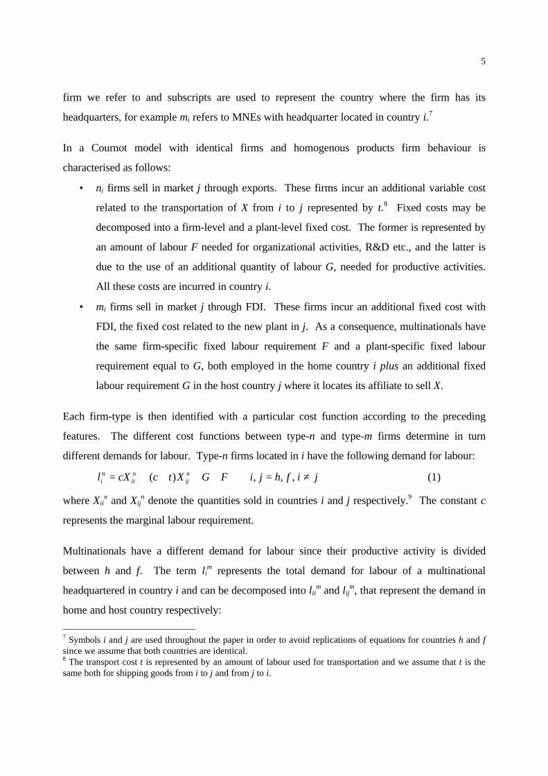
In a Cournot model with identical firms and homogenous products firm behaviour is

characterised as follows:

• ni firms sell in market j through exports. These firms incur an additional variable cost

related to the transportation of X from i to j represented by t.8 Fixed costs may be

decomposed into a firm-level and a plant-level fixed cost. The former is represented by

an amount of labour F needed for organizational activities, R&D etc., and the latter is

due to the use of an additional quantity of labour G, needed for productive activities.

All these costs are incurred in country i.

• mi firms sell in market j through FDI. These firms incur an additional fixed cost with

FDI, the fixed cost related to the new plant in j. As a consequence, multinationals have

the same firm-specific fixed labour requirement F and a plant-specific fixed labour

requirement equal to G, both employed in the home country i plus an additional fixed

labour requirement G in the host country j where it locates its affiliate to sell X.

Each firm-type is then identified with a particular cost function according to the preceding

features. The different cost functions between type-n and type-m firms determine in turn

different demands for labour. Type-n firms located in i have the following demand for labour:

jifhjiFGXtccXl nij

nii

ni ≠=++++= ,,,)( (1)

where Xiin and Xij

n denote the quantities sold in countries i and j respectively.9 The constant c

represents the marginal labour requirement.

Multinationals have a different demand for labour since their productive activity is divided

between h and f. The term lim represents the total demand for labour of a multinational

headquartered in country i and can be decomposed into liim and lij

m, that represent the demand in

home and host country respectively:

7 Symbols i and j are used throughout the paper in order to avoid replications of equations for countries h and fsince we assume that both countries are identical.8 The transport cost t is represented by an amount of labour used for transportation and we assume that t is thesame both for shipping goods from i to j and from j to i.

6

jiandfhjilll mij

mii

mi ≠=+= ,, (2)

jiandfhjiFGcXl mii

mii ≠=++= ,, (3)

jiandfhjiGcXl mij

mij ≠=+= ,, (4)

Accordingly, multinationals avoid transportation costs but incur twice the plant-fixed cost of

national firms since they use a fixed quantity of labour equal to 2G instead of G, the quantity of

labour used by type-n firms.10

The differences in cost functions in turn determines the differences in the relative profitability of

each firm type. With free entry in the market of X, profits are zero so that the relative

performance of each firm-type falls with the number of active firms. All other variables of

interest, such as trade or employment can be derived from the equilibrium number of firms.

Using this theoretical framework, MV show that MNEs (as outlined in appendix 2) will have an

advantage relative to type-n firms when:

1. The overall market is large.

2. The markets are of similar size.

3. Labour costs are similar.

4. Firm-level scale economies are large relative to plant-level scale economies.

5. Transport costs are high.

These results provide a strong basis for the convergence hypothesis since, as noted by Markusen

and Venables (1998, p.196) "convergence of countries h and f in either size or relative

endowments shifts the regime from national to multinational firms."

3 Measuring the convergence hypothesis

From an empirical perspective, the preceding results raise several issues. The first is a problem

common to many empirical analyses of general equilibrium trade models: the models are usually

designed to describe the relationships between two countries, while in the real world, trade and

foreign investment concern a large number of countries (see Bowen et al., 1998). This makes

the model restrictive in applicability but it helps to understand the determinants of FDI, and

9 The equilibrium values for X are given by A.14-A.17 in appendix 1.10 In each country, labour is also employed by type-n firms (with a total demand represented by ni.li

n) and byfirms in Y-sector (LiY). Equation (A3) in the appendix 1 gives the clearing condition in the labour market.

7

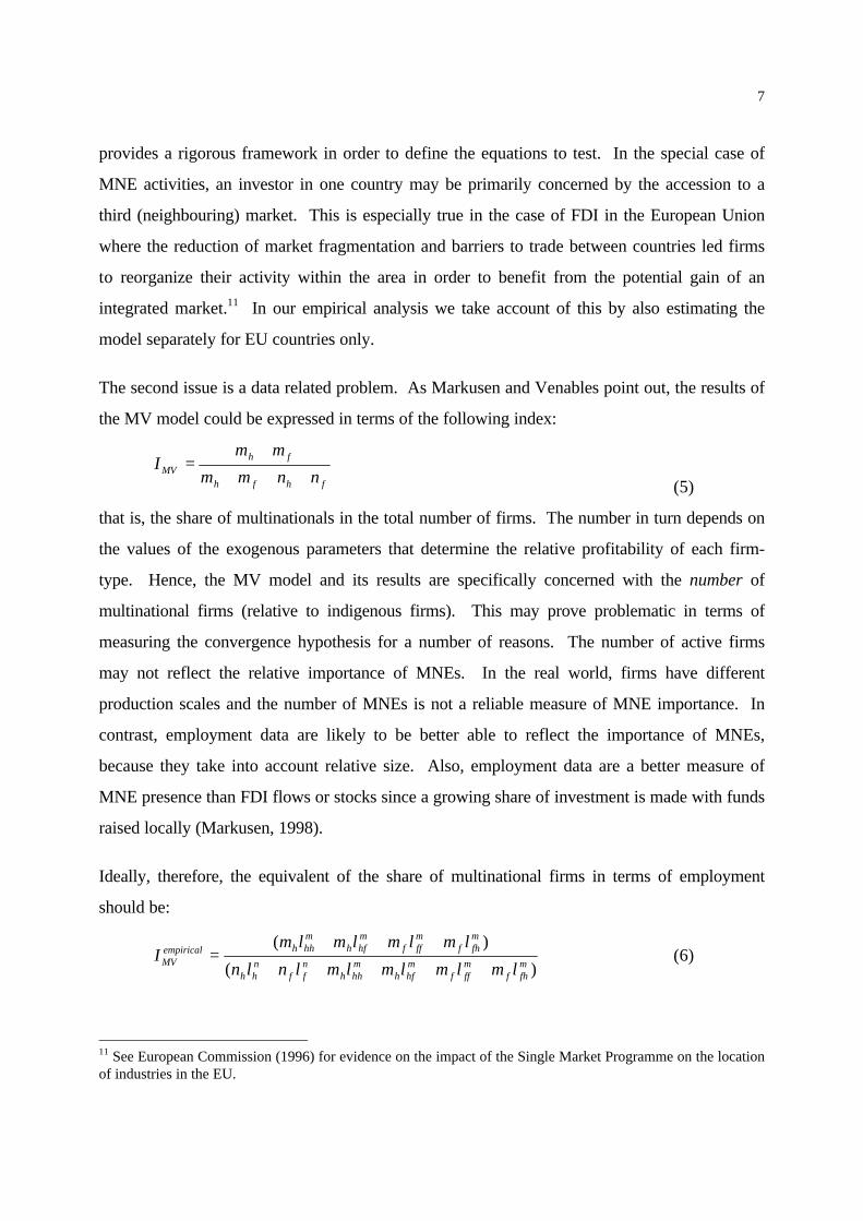
provides a rigorous framework in order to define the equations to test. In the special case of

MNE activities, an investor in one country may be primarily concerned by the accession to a

third (neighbouring) market. This is especially true in the case of FDI in the European Union

where the reduction of market fragmentation and barriers to trade between countries led firms

to reorganize their activity within the area in order to benefit from the potential gain of an

integrated market.11 In our empirical analysis we take account of this by also estimating the

model separately for EU countries only.

The second issue is a data related problem. As Markusen and Venables point out, the results of

the MV model could be expressed in terms of the following index:

fhfh

fhMV nnmm

mmI

+++

+=

(5)

that is, the share of multinationals in the total number of firms. The number in turn depends on

the values of the exogenous parameters that determine the relative profitability of each firm-

type. Hence, the MV model and its results are specifically concerned with the number of

multinational firms (relative to indigenous firms). This may prove problematic in terms of

measuring the convergence hypothesis for a number of reasons. The number of active firms

may not reflect the relative importance of MNEs. In the real world, firms have different

production scales and the number of MNEs is not a reliable measure of MNE importance. In

contrast, employment data are likely to be better able to reflect the importance of MNEs,

because they take into account relative size. Also, employment data are a better measure of

MNE presence than FDI flows or stocks since a growing share of investment is made with funds

raised locally (Markusen, 1998).

Ideally, therefore, the equivalent of the share of multinational firms in terms of employment

should be:

)(

)(mfhf

mfff

mhfh

mhhh

nff

nhh

mfhf

mfff

mhfh

mhhhempirical

MV lmlmlmlmlnln

lmlmlmlmI

+++++

+++= (6)

11 See European Commission (1996) for evidence on the impact of the Single Market Programme on the locationof industries in the EU.

8

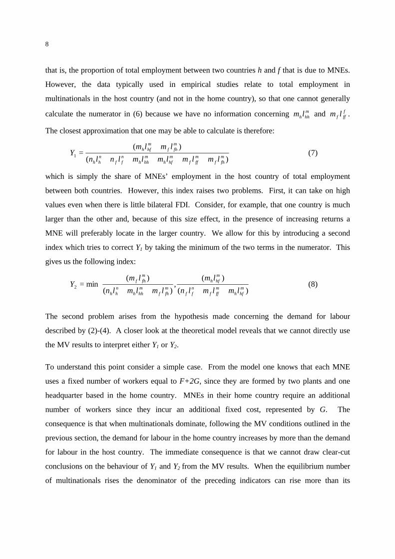
that is, the proportion of total employment between two countries h and f that is due to MNEs.

However, the data typically used in empirical studies relate to total employment in

multinationals in the host country (and not in the home country), so that one cannot generally

calculate the numerator in (6) because we have no information concerning mhhhlm and f

fff lm .

The closest approximation that one may be able to calculate is therefore:

)(

)(1 m

fhfmfff

mhfh

mhhh

nff

nhh

mfhf

mhfh

lmlmlmlmlnln

lmlmY

+++++

+= (7)

which is simply the share of MNEs’ employment in the host country of total employment

between both countries. However, this index raises two problems. First, it can take on high

values even when there is little bilateral FDI. Consider, for example, that one country is much

larger than the other and, because of this size effect, in the presence of increasing returns a

MNE will preferably locate in the larger country. We allow for this by introducing a second

index which tries to correct Y1 by taking the minimum of the two terms in the numerator. This

gives us the following index:

++++=

)(

)(,

)(

)(min2 m

hfhmfff

nff

mhfh

mfhf

mhhh

nhh

mfhf

lmlmln

lm

lmlmln

lmY (8)

The second problem arises from the hypothesis made concerning the demand for labour

described by (2)-(4). A closer look at the theoretical model reveals that we cannot directly use

the MV results to interpret either Y1 or Y2.

To understand this point consider a simple case. From the model one knows that each MNE

uses a fixed number of workers equal to F+2G, since they are formed by two plants and one

headquarter based in the home country. MNEs in their home country require an additional

number of workers since they incur an additional fixed cost, represented by G. The

consequence is that when multinationals dominate, following the MV conditions outlined in the

previous section, the demand for labour in the home country increases by more than the demand

for labour in the host country. The immediate consequence is that we cannot draw clear-cut

conclusions on the behaviour of Y1 and Y2 from the MV results. When the equilibrium number

of multinationals rises the denominator of the preceding indicators can rise more than its

9

numerator depending on how MNE’s employment in their home country behaves with respect

to national firms employment. The model does not provide a clear answer on this and we have

to rely on the empirical estimates provided in the next section.

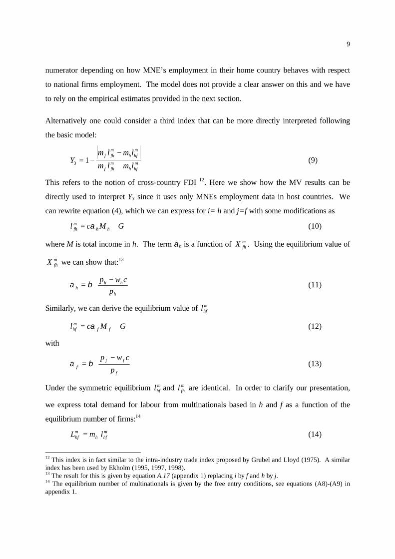
Alternatively one could consider a third index that can be more directly interpreted following

the basic model:

Ym l m l

m l m lf fh

mh hf

m

f fhm

h hfm3 1= −

−

+(9)

This refers to the notion of cross-country FDI 12. Here we show how the MV results can be

directly used to interpret Y3 since it uses only MNEs employment data in host countries. We

can rewrite equation (4), which we can express for i= h and j=f with some modifications as

GMcl hhmfh += α (10)

where M is total income in h. The term αh is a function of mfhX . Using the equilibrium value of

mfhX we can show that:13

h

hhh p

cwp −= βα (11)

Similarly, we can derive the equilibrium value of mhfl

GMcl ffmhf += α (12)

with

f

fff p

cwp −= βα (13)

Under the symmetric equilibrium mhfl and m

fhl are identical. In order to clarify our presentation,

we express total demand for labour from multinationals based in h and f as a function of the

equilibrium number of firms:14

mhfh

mhf lmL = (14)

12 This index is in fact similar to the intra-industry trade index proposed by Grubel and Lloyd (1975). A similarindex has been used by Ekholm (1995, 1997, 1998).13 The result for this is given by equation A.17 (appendix 1) replacing i by f and h by j.14 The equilibrium number of multinationals is given by the free entry conditions, see equations (A8)-(A9) inappendix 1.

10

mfhf

mfh lmL = (15)

In order to see how Y3 behaves with the exogenous variables of the model, we use the type of

analysis carried out by MV to derive our results concerning mhfL and m

fhL for five cases; the

impact of a change in (i) total income, (ii) the distribution of income, (iii) factor proportions,

(iv) plant versus firm-fixed costs and (v) transport costs. As in MV, we assume that countries h

and f are identical, which implies that, initially, commodity and factor prices as well as income,

are identical in both countries.15

Case 1: Change in total income: 0>= fh dMdM

The impact on mhfL and m

fhL can be represented by:

0)( >++=+= hhhffmhfhh

mhf

mhf cmdmGMcdlmdmldL αα

0)( >++=+= fffhhmfhff

mfh

mfh cmdmGMcdlmdmldL αα

Following MV, we have 0>= fh dmdm since the relative profitability of multinationals rises

compared to national firms. With a positive number of mh and mf firms, the other components

are all positive.

We can then write:

00 3 >⇒>= dYdMdM fh

Case 2: Change in the distribution of income: 0>−= fh dMdM

The impact on mhfL and m

fhL is as follows:

00 >+=+= hhmhfhh

mhf

mhf cmdlmdmldL α

00 <+−=+= hhmfhff

mfh

mfh cmdlmdmldL α

The equilibrium values of mh and mf are not affected by this change and the change in mhfl and m

fhl

is exactly opposite given that countries are symmetric in all respects. Accordingly, the

15 All changes affecting the equilibrium number of firms in the five cases considered here are explained in moredetail in appendix 2.

11

numerator of Y3 does not change but the denominator rises. The final outcome is a decrease in

Y3:

00 3 <⇒>−= dYdMdM fh

Case 3: Change in unit labour cost: 0>−= hf dwdw with i=f and j=h.

This change can be equally considered as a change in factor proportions:

0>

∆−=

∆

RL

dRL

d

with: 0(.)'',0(.)'0)0( =∆>∆=∆

∆=−= andand

RL

R

w

r

ww

j

j

i

iδ

Here the impact is straightforward since αh and αf are descreasing function of wh and wf

respectively: 0>mhfdL and 0<m

fhdL and Y3 falls, we can then state that:

00 3 <⇒>−= dYdwdw hf

Case 4: Change in firm versus plant cost ratio: 0>−= dGdF

The symmetric change is in fact used by MV to get a relative measure of the change in the

relative profitability of type-m firms vs. type-n firms. Type-n firms are not directy affected since

their losses (dF>0) are exactly identical to their gains (–dG>0), so that total fixed costs do not

change. For MNEs, however, total fixed cost falls and the relative profitability of MNEs rises

compared to national firms. There is a dual effect on labour demand since foreign affiliates

lower their use of labour (because of -dG ), while the number of active MNEs increases

following MV. We have:

hhmhf

mhf mdmldL −=

ffmfh

mfh mdmldL −=

The final outcome depends on the relative values of jiandhfiwithmanddml iimij ≠= , .

As a consequence, the model does not yield unambiguous results as to whether the numerator

of Y3 will increase or decrease with such a symmetric change.

12

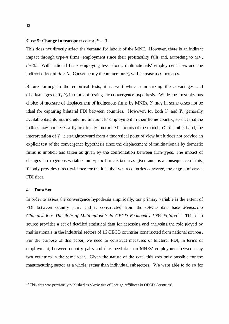
Case 5: Change in transport costs: dt > 0

This does not directly affect the demand for labour of the MNE. However, there is an indirect

impact through type-n firms’ employment since their profitability falls and, according to MV,

dn<0. With national firms employing less labour, multinationals’ employment rises and the

indirect effect of dt > 0. Consequently the numerator Y3 will increase as t increases.

Before turning to the empirical tests, it is worthwhile summarizing the advantages and

disadvantages of Y1-Y3 in terms of testing the convergence hypothesis. While the most obvious

choice of measure of displacement of indigenous firms by MNEs, Y1 may in some cases not be

ideal for capturing bilateral FDI between countries. However, for both Y1 and Y2, generally

available data do not include multinationals’ employment in their home country, so that that the

indices may not necessarily be directly interpreted in terms of the model. On the other hand, the

interpretation of Y3 is straightforward from a theoretical point of view but it does not provide an

explicit test of the convergence hypothesis since the displacement of multinationals by domestic

firms is implicit and taken as given by the confrontation between firm-types. The impact of

changes in exogenous variables on type-n firms is taken as given and, as a consequence of this,

Y3 only provides direct evidence for the idea that when countries converge, the degree of cross-

FDI rises.

4 Data Set

In order to assess the convergence hypothesis empirically, our primary variable is the extent of

FDI between country pairs and is constructed from the OECD data base Measuring

Globalisation: The Role of Multinationals in OECD Economies 1999 Edition.16 This data

source provides a set of detailed statistical data for assessing and analysing the role played by

multinationals in the industrial sectors of 16 OECD countries constructed from national sources.

For the purpose of this paper, we need to construct measures of bilateral FDI, in terms of

employment, between country pairs and thus need data on MNEs’ employment between any

two countries in the same year. Given the nature of the data, this was only possible for the

manufacturing sector as a whole, rather than individual subsectors. We were able to do so for

16 This data was previously published as ‘Activities of Foreign Affiliates in OECD Countries’.

13

27 country pairs over a number of years, providing us with a data sample size of 118 for which

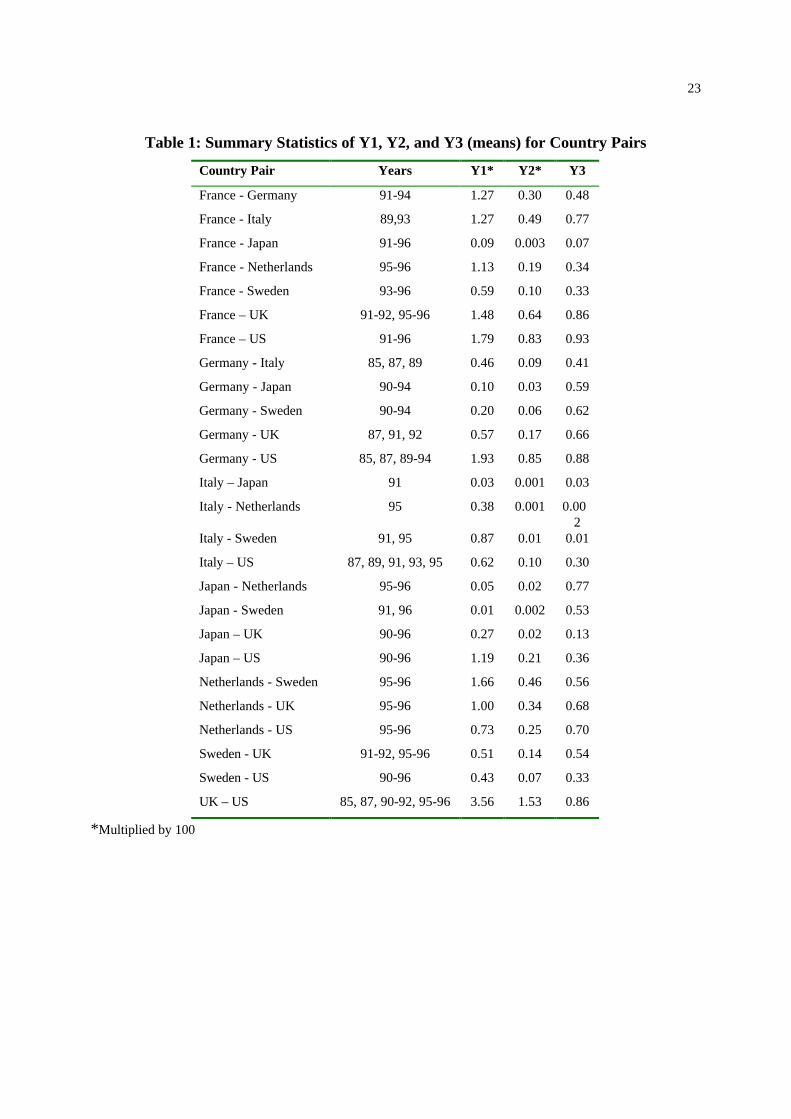
we have provided summary statistics in Table 1.

As can be seen, there is a considerable variety of country pairs, all of which are between

developed countries. The sample years and size also differs for each country pair. For example

our proxy for bilateral FDI, Y1, varies considerably across these, from 1.66 to 0.01, for

Netherlands-Sweden and Japan-Sweden, respectively.17 The correlation coefficient between Y1

and Y2 is 0.96, implying that may be a good proxy for both displacement of indigenous industry

by MNEs and bilateral FDI. In contrast, the correlation coefficient between Y3 and Y1 and Y2 is

0.69 and 0.55, respectively. Thus this measure of bilateral FDI may not be a particularly good

proxy for displacement.

[Table 1 here]

5 Econometric Methodology

In order to estimate empirically the effect of the above factors on the intensity of cross-direct

investment we use the following basic model,18

Yij = β0 + β1[ln(GDPi)+ln(GDPj)] + β2(abs(GDPi-GDPj)) + β3((abs(SENDi-SENDj)) + + β

4((abs(CENDi-CENDj)) + β5[ln(RDi)+ln(RDj)] + β6(DISTij) + β7(LANGij) + eij (16)

where Yij is two-way multinational activity between countries i and j measured in terms of

employment using the three indices discussed in Section 3, GDPs is gross domestic product of

country s = i,j, SENDs is country s’ relative endowment of skilled labour, CENDs is country s’

relative endowment of physical capital, RDs is a proxy of country s’ research intensity, DISTij is

the distance between the capitals of i and j, and LANGij is a dummy variable set equal to one if

countries i and j have a common language.

The first four terms on the right hand side of the equation relate to size and relative

endowments. They are included to test the predictions that multinational employment between

17 For both the summary statistics and the regression results we have multiplied both Y1 and Y2 by 100.18 The definition of the explanatory variables and their data sources are summarised in appendix 3.

14

two countries increases as (i) total market size increases and countries grow more similar in (ii)

size and (iii) relative endowments. We measure relative endowments of skilled workers using

two alternative proxies, (i) the share of employment in R&D activity relative to total

employment in the country, and (ii) the percentage of students enrolled in secondary school

education in the total population in the country. Relative physical capital endowments are

measured as per capita capital stock in the country.

The MV model also predicts that multinational employment can be expected to be more

important if firm-level scale economies are large. Therefore, R&D intensity is included to proxy

the importance of firm-level scale economies. A country pair’s R&D intensity is calculated as

the sum of each country’s per capita R&D expenditures. This in some way captures the

"knowledge-capital model" referred to by Markusen (1995) in which multinationals are seen as

firms exploiting some ownership advantage through investment abroad. The ability to exploit

such advantages is more likely in industries in which knowledge intensive production is

important. As a consequence, multinationals are associated with high ratios of R&D relative to

sales and employ a large proportion of qualified workers. From an empirical perspective this

implies that multinationals are more likely to exist in countries were industry is R&D-intensive.

In the MV model this variable corresponds to F, the firm-specific fixed cost.

Furthermore, the MV model suggests that multinationals can be assumed to be important

relative to national firms if transport costs and trade barriers are high. We include the distance

between the two countries as a rough proxy in the empirical formulation to take account of this.

Finally, the equation also includes a dummy variable set equal to one if countries share a

common language, since a common language can be assumed to reduce transaction costs of

setting up subsidiaries abroad and should, therefore, favour multinational production.

It should be noted that equation (16) is similar to a gravity equation as used in empirical work in

international trade (see, for example, Bergstrand, 1985, McCallum, 1995, Frankel et al., 1998)

and, more recently, in the analysis of the activities of multinational companies (Ekholm, 1995,

1997, 1998, Brainard, 1997, Markusen and Maskus, 1999, Carr et al., 2000). While the

theoretical foundations for using gravity equations in trade are, however, debatable (see

15

Deardorff, 1984 and Evenett and Keller, 1998) the MV model appears to provide a coherent

theoretical framework for the use of gravity equations for the analysis of the activities of

multinational companies.

6 Econometric Results

Our results for estimating (16) using standard OLS techniques for our total sample for the

indices Y1, Y2 and Y3 are given in Table 2.19 For all three indices we find that total market size

(GDP) and the absolute difference in relative market size (ABSGDP), are significantly positive

and negative determinants of bilateral multinational activity, although in the case of Y3,

ABSGDP does not turn out to be statistically significant. Despite this the results are in line with

the convergence hypothesis, i.e., the share of bilateral FDI of total manufacturing employment

of country pairs increases as total market size increases and as countries become more similar in

size.

[Table 2 here]

The evidence on the effect of differences in relative endowments is less clear-cut, however.

While the first proxy of endowments of skilled workers, SEND1, is statistically insignificant in

all specifications, SEND2 turns out to be significantly negative in the case of Y1 but positive and

significant in the case of Y3. Differences in physical capital intensity turn out positive in all

specifications but are only statistically significant in those that utilise SEND2. We thus find

evidence for the convergence hypothesis in terms of relative endowments only for the

specification using Y1 and SEND2 (as proxy of relative human capital endowments) and even in

that case, the proxy of physical capital endowments is not as one would expect.20,21

19 One could argue that given the panel nature of our data set that perhaps we should have controlled for countrypair fixed effects. However, we chose not to do so for two reasons. Firstly, given our sample size and the largenumber of country pairs this would have considerably reduced the degrees of freedom. Secondly, given that foreach country pair the time period covered is generally only a few years and many of our explanatory variables,such as relative market size or relative factor endowments, will not have varied to any great extent over shorttime periods, controlling for country pair fixed effects would have purged from our equation exactly what we aretrying to measure. Hence, our estimation always assumes that country pair specific fixed unobservables are notcorrelated with the explanatory variables.20 We also re-ran the regressions including only one measure of resource endowments, i.e., either SEND1,SEND2 or CEND. The results, which are not reported here, are qualitatively similar to the ones reported herein,however.21 One should note, however, that Markusen (1998) in his review of the literature also states that, "a high volumeof outward direct investment is positively related to a country's endowment of skilled labour and insignificantly

16

In all specifications, we find a positive and significant coefficient on the proxy for firm level

economies of scale, RD. As noted earlier, the nature of our independent variable did not allow

us, within the framework of the MV model, to predict a priori what effect this proxy for the

importance of firm-level fixed costs would have on bilateral FDI. However, our results indicate

that the relationship is clearly positive and statistically significant.

Our results also show that countries with a common language experience greater bilateral FDI.

In contrast, the greater the distance between two country’s capitals the lower is bilateral FDI.

This latter result is contrary to the convergence hypothesis. However, Markusen (1998, p. 736)

notes that there is weak evidence that FDI is primarily motivated by the avoidance of tariffs or

measurable transport costs. This may be particularly the case for vertical FDI, where the

production of intermediate goods is in low-cost locations but the final good is assembled in the

home country. In this case, the multinational may wish to locate as near as possible to the home

country to avoid transportation costs for shipping the intermediate good between host and home

country. Also, Brenton et al. (1999) note that distance may be negatively related to FDI since

the costs of operating overseas are likely to rise with distance because of, for example, higher

communication costs and higher costs of placing personnel abroad.

The opposite sign we report for distance could possibly be due to the fact that our sample

contains mainly European firms with strong cross-investment during the period under study.22

Moreover, the distance between countries may not be a perfect proxy for transport costs. For

instance, it may also reflect cultural differences between countries - countries that are further

apart may also be culturally more distinct from each other and, as Kumar (2000) finds for US

and Japanese FDI, foreign investment is positively related to cultural proximity.

or negatively related to its physical capital endowment" (p. 736).22 The increased level of integration has translated into a significant decrease in barriers for goods, services andfactor movements within the Union, lowering the segmentation of markets and enhancing the rationalization ofproduction as noted by Muchielli and Burgenmeier (1991). The fall in trade barriers may act in favour ofvertical FDI since intermediate goods are more easily traded within the firm. The fact that investment occursbetween developed countries means that there is still a scope for production rationalization and costminimization within the firm even if labour costs are similar between locations. Labour skills may be diversifiedacross countries or regions and this in turn may provide a rationale for relocation of productive activities whentrade barriers are being removed. On the other hand, factor costs may still be different between industrializedcountries, even if those differences are lower than comparing to developing countries. The combination of lowinternal barriers to trade and still high barriers to external trade may provide a valid reason for cost reduction

17

Part of the drawback of estimating (16) for our total sample of country pairs is that we are

pooling within EU, across the EU and outside the EU data. The nature of bilateral FDI may,

however, be intrinsically different for country pairs within these three groupings. To examine

how this may affect our results we also sub-divided our sample into those with bilateral FDI

within the EU and those for which at least one country was not in the EU at the time. Note,

however, that particularly for the EU sample, all results must be viewed with some caution

given the relatively small sample size.

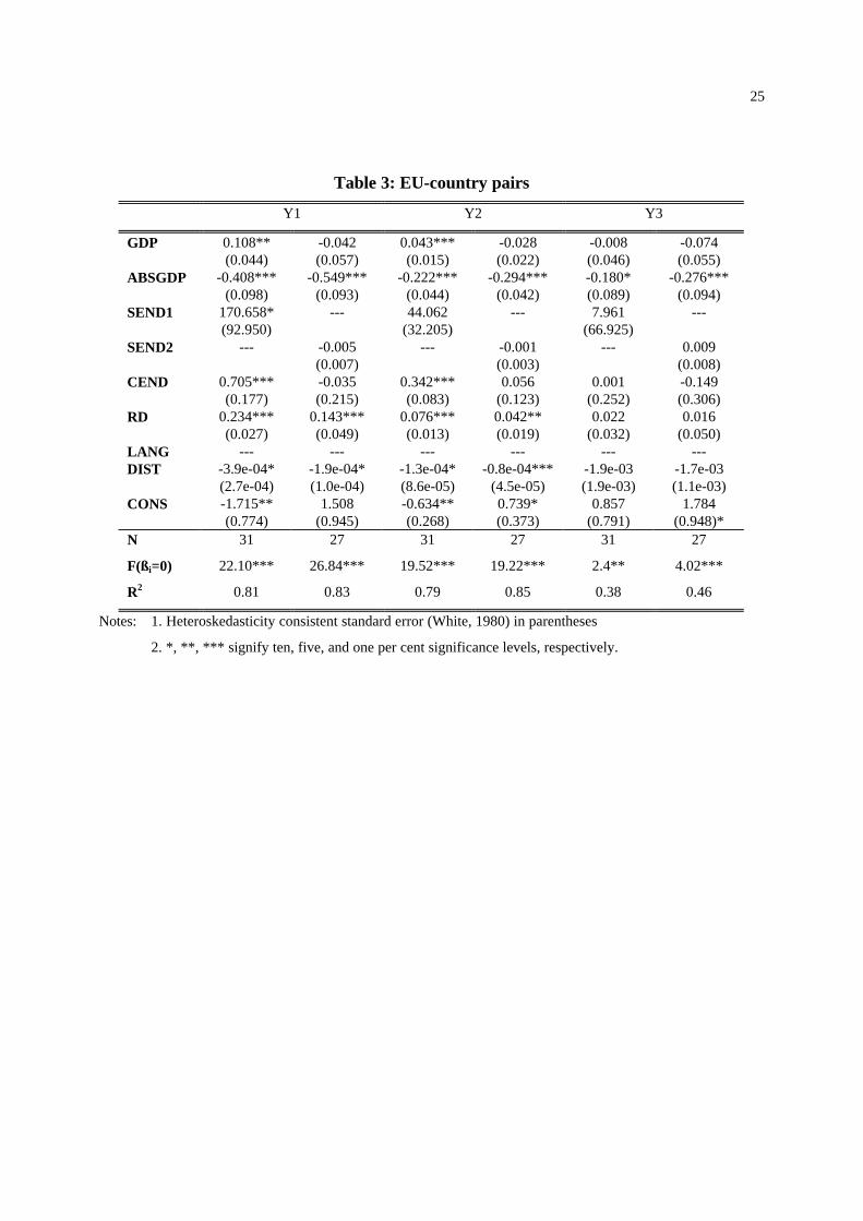
The results for estimating (16) for the sample of EU country pairs only are given in Table 3.

Reducing our sample to bilateral FDI within the EU does not alter our results in terms of

relative market size, distance or R&D intensity, although the coefficients on distance and R&D

intensity turn out to be statistically insignificant in the case of Y3.23 Total market size also turns

only out to be statistically significant and positive in two out of six cases. In terms of relative

factor endowments we find that both SEND1 and CEND are statistically significant for the

dependent variable Y1, but both have a positive effect. Differences in physical capital

endowments also turn out to be positive and statistically significant for Y2, although the proxies

for human capital endowments are statistically insignificant in that case.

[Table 3 here]

For the non-EU sample, the results of which are reported in Table 4, the proxy for differences in

physical capital endowments are statistically insignificant in all specifications, while differences

in country size and the proxy for R&D intensity are only significant in one and three

specifications respectively although with similar signs as in the overall sample. Our findings are

much in line with the overall sample, however, for total market size, human capital endowments,

language and distance variables.

[Table 4 here]

The consistently negative and statistically significant sign on the distance variable in all

specifications is particularly puzzling. The MV model clearly predicts that multinationals

through FDI in low-wages countries when factor intensities between stages of production differ.23 The language dummy is dropped for the EU sample because none of the country pairs share a commonlanguage.

18

become relatively more important as transport costs increase, but, assuming that transport costs

increase with distance, our results suggest the opposite – closeness favours FDI. As pointed

out above, distance may not be a perfect proxy for transport costs, however. In the absence of

detailed data on the actual level of transport costs between countries, we, therefore, in an

extension to the basic empirical model replace the distance variable with an indicator of the

importance of trade flows between two countries. This may serve as a proxy for transport costs

if we assume that countries trade more the lower are transport costs. Specifically, we calculate

the variable as )()( jiijijij GDPGDPMXOPEN ++= where Xij are exports from country i to j,

and Mij are imports into country i from country j.

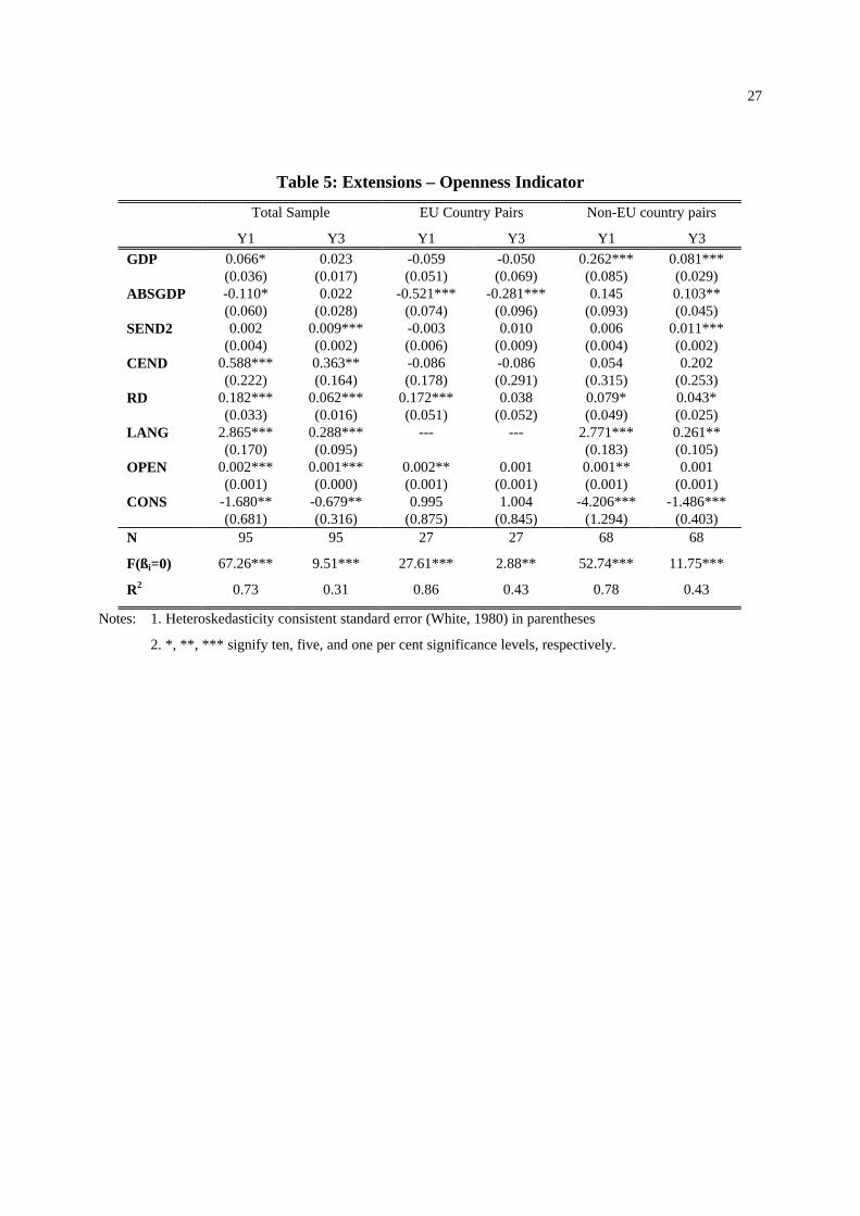
The results are reported in Table 5. Overall these are similar to the results reported previously

and we find that the trade variable has a positive sign and is statistically significant in four out of

six cases. This is again in contrast with the MV model, which predicts that high transport costs

favour FDI. The positive sign then provides further evidence that this relationship is more

complex for a number of reasons – not least because trade and FDI may be complements rather

than substitutes (Markusen, 1983).

[Table 5 here]

In the estimations thus far we have assumed that it is the size of the individual country that

matters. Arguably, however, it may be the case that for EU countries it is not the size of the

individual EU member country, but the size of the total EU that attracts FDI (both from extra-

EU and intra-EU sources) to serve the large EU market (see Görg and Ruane, 1999 for a

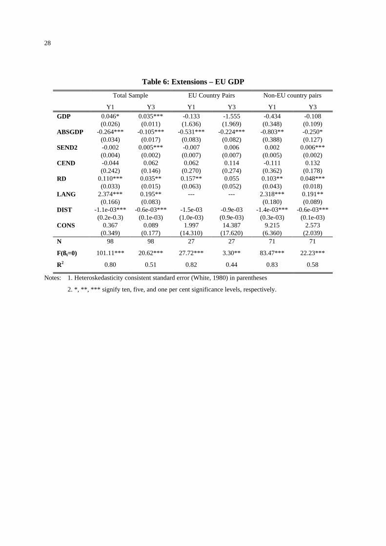
discussion). In an alternative specification we re-calculated both GDP and ABSGDP to take

account of this. GDP is calculated as total EU GDP if we analyse a pair of EU countries, the

sum of total EU GDP and individual country GDP in the case of one EU country and one non-

EU country, and the sum of individual country GDP for two non-EU countries. ABSGDP is

calculated as the difference between EU GDP and country GDP in the case of one EU and one

non-EU country. Otherwise, it is calculated as the difference of individual country’s GDPs.

The results of the estimations using these measures are presented in Table 6. While the

coefficients on ABSGDP are negative and statistically significant as expected in all cases, the

19

results on the GDP variable are rather disappointing. While it turns out to be statistically

significant and positive for the total sample, breaking the sample up into EU country pairs and

non-EU country pairs yields statistically insignificant results in all cases. Assuming the

convergence hypothesis is correct, this casts doubt on the assertion that it is the total EU market

size, rather than individual country size that matters for investment decisions, although again we

have to be cautious in drawing conclusions due to the small sample sizes, particularly for the EU

sample.

[Table 6 here]

7 Conclusion

In this paper we investigate whether multinational companies tend to displace indigenous firms

and trade as countries become more similar in size, factor endowments and production costs

and as total market size increases. To do so we explicitly relate our empirical measures of

bilateral FDI between two countries to a recent theoretical model developed by Markusen and

Venables (1998). We set out to test this for a panel of OECD country pairs over the period

1985-96.

Our results support the convergence hypothesis to some extent. Overall market size tends to

increase, while differences in market size tend to reduce bilateral MNE activity. While the role

of differences in relative endowments of human or physical capital skilled workers is not clear

from our results, R&D intensity, which serves to proxy the importance of firm level scale

economies, and a common language in home and host country significantly increase bilateral

MNE activity. We also find that for many cases transportation costs, contrary to the

convergence hypothesis, are negative determinants, although these findings are in line with

similar findings in the literature. Breaking down our sample into EU and non-EU pairs we only

find that a large number of our results in aggregate still hold, although, given the small sample

size, particularly for EU country pairs, these results must be viewed with some caution.

20

References

Barrell, R. and Pain, N. 1996, “An Econometric Analysis of U.S. Foreign Direct Investment”,Review of Economics and Statistics, Vol. 78, pp. 200-207.

Barrell, R. and Pain, N. 1999, “Domestic Institutions, Agglomerations and Foreign DirectEuropean Economic Review, Vol. 43, pp. 925-934.

Bergstrand, J.H. 1985, “The Gravity Equation in International Trade: Some MicroeconomicFoundations and Empirical Evidence”, Review of Economics and Statistics, Vol. 67, pp.474-481.

Bowen H.P., Holander, A. and Viaene, J.M. (ed.) 1998, Applied International Trade Analysis,London: MacMillan.

Brainard, S.L. 1993, A simple theory of multinational corporations and trade with a trade-offbetween proximity and concentration, NBER working paper 4269.

Brainard, S.L. 1997, “An Empirical Assessment of the Proximity-Concentration Trade-offbetween Multinational Sales and Trade”, American Economic Review, Vol. 87, pp. 520-544.

Brenton, P., Di Mauro, F. and Lücke, M. 1999, “Economic Integration and FDI: An EmpiricalAnalysis of Foreign Investment in the EU and in Central and Eastern Europe”,Empirica, Vol. 26, pp. 95-121.

Carr, D.L., Markusen, J.R. and Maskus, K.E. 2000, “Estimating the Knowledge-Capital Modelof the Multinational Enterprise”, American Economic Review, forthcoming.

Culem, C.G. 1988, “The Locational Determinants of Direct Investments among IndustrializedEuropean Economic Review, Vol. 32, pp. 885-904.

Deardorff, A.V. 1984, “Testing Trade Theories and Predicting Trade Flows”, in: Jones, R. andKenen, P. (eds), Handbook of International Economics Vol. 1 (Amsterdam: Elsevier),pp. 467-517.

Dunning, J.H. 1977, “Trade, Location of Economic Activity and MNE: A search for an EclecticOhlin, B. Hesselborn, P.O. and Wijkman, P.M. (eds), The International

Allocation of Economic Activity (London, MacMillan), pp. 395-418.Ekholm, K. 1995, “Multinational Production and Trade in Technical Knowledge”. Lund

Economic Studies No. 58, Lund.Ekholm, K. 1997, “Factor Endowments and the Pattern of Affiliate Production by Multinational

Enterprises”, CREDIT Research Paper 97/19, University of Nottingham.Ekholm, K. 1998, “Proximity Advantages, Scale Economies, and the Location of Production”,

in: Pontus Braunerhjelm and Karolina Ekholm (eds.), The Geography of Multinationals(Kluwer Academic Publishers, Dordrecht), pp. 59-76.

Ethier, W.J. 1986, “The multinational firm”, Quarterly Journal of Economics, Vol. 80, pp. 805-834.

European Commission 1996, Economic Evaluation of the Internal Market, European Economyno4, Directorate General for Economic and Financial Affairs, Brussels.

21

Evenett, S.J. and Keller, W. 1998, On Theories Explaining the Success of the Gravity Equation,NBER working paper 6529.

Falvey, Rod E. 1981, “Commercial Policy and Intra-Industry Trade”, Journal of InternationalEconomics, Vol. 11, pp. 495-511.

Frankel, J.; Stein, E. and Wei, S. 1998, “Continental trading blocs: are they natural orsupernatural?”, in J. Frankel (ed.), The Regionalization of the World Economy. ChicagoUniversity Press, Chicago, pp. 91-113.

Görg, H. and Ruane, F. 1999, „US Investment in EU Member Countries: The Internal Marketand Sectoral Specialization”, Journal of Common Market Studies, Vol. 37, pp. 333-348.

Grubel, H.G. and Lloyd, P.J. 1975, Intra Industry Trade, Macmillan: London.Head, K.; Ries, J. and Swenson, D. 1995, “Agglomeration Benefits and Location Choice:

Evidence from Japanese Manufacturing Investments in the United States”, Journal ofInternational Economics, Vol. 38, pp. 223-247.

Helpman, E.M. 1984, “A simple theory of international trade with multinational corporations”,Journal of Political Economy, Vol. 92, pp. 451-471.

Helpman, E.M. 1985, “Multinational corporations and trade structure”, Review of EconomicStudies, Vol. 52, pp. 443-457.

Helpman, E.M. and Krugman, P.R. 1985, Market Structure and Foreign Trade, Cambridge,MIT Press (ed.).

Kravis, I.B. and Lipsey, R.E. 1982, “The Location of Overseas Production and Production forExport by U.S. Multinational Firms”, Journal of International Economics, Vol. 12, pp.201-223.

Krugman, P.R. 1979, “Increasing returns, Monopolistic Competition, and International Trade”,Journal of International Economics, Vol. 9, pp.469-480.

Kumar, N. 2000, “Explaining the Geography and Depth of International Production: The Caseof US and Japanese Multinational Enterprises”, Weltwirtschaftliches Archiv, Vol. 136,pp. 442-477.

Markusen, J.R. 1983, "Factor Movements and Commodity Trade as Complements". Journal ofInternational Economics. Vol. 14. pp. 341-356.

Markusen, J.R. 1984, “Multinationals, multi-plant economies and the gains from trade”, Journalof International Economics, Vol. 16, pp.205-226.

Markusen, J.R. 1995, “The boundaries of Multinational Enterprises and the Theory ofJournal of Economic Perspectives, Vol. 9, pp.169-189.

Markusen, J.R. 1998, “Multinational Firms, Location and Trade”, World Economy, Vol. 21, pp.733-56.

Markusen, J.R. and Maskus, K.E. 1999, “Multinational Firms: Reconciling Theory andEvidence”, NBER Working Paper 7163.

Markusen, J.R. and Venables, A.J. 1996, “The Increased Importance of Direct Investment inNorth Atlantic Economic Relationships: A Convergence Hypothesis”, in Cazoneri, M.,

22

Ethier, W., and Grilli, V. (eds.), The New Transatlantic Economy (CambridgeUniversity Press: Cambridge).

Markusen, J.R. and Venables, A.J. 1998, “Multinational Firms and the New Trade Theory”,Journal of International Economics, Vol. 46, pp. 183-203.

McCallum, J. 1995, “National borders matter: Canada-U.S. regional trade patterns”, AmericanEconomic Review, Vol. 85, pp. 615-623.

Muchielli, J.L. and Burgenmeier, B. 1991, Multinationals and Europe 1992: Strategies for thefuture, London, Routledge.

Organisation for Economic Co-Operation and Development, 1999(a), MeasuringGlobalisation: The role of multinationals in OECD economies, OECD, Paris.

Organisation for Economic Co-Operation and Development, 1999(b), Science, Technology andIndustry Scoreboard, Benchmarking Knowledge based economies, OECD, Paris.

Organisation for Economic Co-Operation and Development 1999(c), Research andDevelopment Expenditure in Industry, OECD, Paris.

United Nations 1997, International Trade Statistics Yearbook, U.N. New York.United Nations 1999, World Investment Report, U.N. New York.Wheeler, D.and Mody, A. 1992, “International Investment Location Decisions”, Journal of

International Economics, Vol. 33, pp. 57-76.

23

Table 1: Summary Statistics of Y1, Y2, and Y3 (means) for Country Pairs

Country Pair Years Y1* Y2* Y3

France - Germany 91-94 1.27 0.30 0.48

France - Italy 89,93 1.27 0.49 0.77

France - Japan 91-96 0.09 0.003 0.07

France - Netherlands 95-96 1.13 0.19 0.34

France - Sweden 93-96 0.59 0.10 0.33

France – UK 91-92, 95-96 1.48 0.64 0.86

France – US 91-96 1.79 0.83 0.93

Germany - Italy 85, 87, 89 0.46 0.09 0.41

Germany - Japan 90-94 0.10 0.03 0.59

Germany - Sweden 90-94 0.20 0.06 0.62

Germany - UK 87, 91, 92 0.57 0.17 0.66

Germany - US 85, 87, 89-94 1.93 0.85 0.88

Italy – Japan 91 0.03 0.001 0.03

Italy - Netherlands 95 0.38 0.001 0.002

Italy - Sweden 91, 95 0.87 0.01 0.01

Italy – US 87, 89, 91, 93, 95 0.62 0.10 0.30

Japan - Netherlands 95-96 0.05 0.02 0.77

Japan - Sweden 91, 96 0.01 0.002 0.53

Japan – UK 90-96 0.27 0.02 0.13

Japan – US 90-96 1.19 0.21 0.36

Netherlands - Sweden 95-96 1.66 0.46 0.56

Netherlands - UK 95-96 1.00 0.34 0.68

Netherlands - US 95-96 0.73 0.25 0.70

Sweden - UK 91-92, 95-96 0.51 0.14 0.54

Sweden - US 90-96 0.43 0.07 0.33

UK – US 85, 87, 90-92, 95-96 3.56 1.53 0.86

*Multiplied by 100

24

Table 2: Total Sample

Y1 Y2 Y3

GDP 0.264***(0.049)

0.257***(0.047)

0.135***(0.024)

0.121***(0.021)

0.107***(0.025)

0.095***(0.025)

ABSGDP -0.150***(0.054)

-0.176***(0.047)

-0.048**(0.022)

-0.060***(0.020)

-0.012(0.023)

-0.012(0.020)

SEND1 15.988(29.030)

--- 3.374(15.009)

--- -19.363(24.230)

---

SEND2 --- -0.006***(0.003)

--- -0.002(0.002)

--- 0.005***(0.002)

CEND 0.316(0.205)

0.405**(0.178)

0.131(0.092)

0.243***(0.082)

0.106(0.116)

0.262**(0.134)

RD 0.190***(0.032)

0.187***(0.030)

0.068***(0.015)

0.077***(0.015)

0.039***(0.014)

0.060***(0.015)

LANG 2.518***(0.129)

2.543***(0.120)

1.152***(0.070)

1.192***(0.074)

0.273***(0.063)

0.306***(0.086)

DIST -1.2e-04***(1.49e-05)

-1.2e-04***(1.31e-05)

-5.3e-05***(7.76e-06)

-5.1e-05***(7.31e-06)

-5.0e-04***(1.0e-04)

-4.7e-04***(1.1e-04)

CONS -3.481***(0.618)

-3.223***(0.637)

-1.806***(0.319)

-1.732***(0.303)

-0.987***(0.337)

-1.159***(0.314)

N 105 98 105 98 105 98

F(ßi=0) 103.86*** 129.93*** 88.98*** 75.06*** 12.16*** 12.88***

R2 0.80 0.85 0.76 0.81 0.38 0.45

Notes: 1. Heteroskedasticity consistent standard error (White, 1980) in parentheses

2. *, **, *** signify ten, five, and one per cent significance levels, respectively.

25

Table 3: EU-country pairs

Y1 Y2 Y3

GDP 0.108**(0.044)

-0.042(0.057)

0.043***(0.015)

-0.028(0.022)

-0.008(0.046)

-0.074(0.055)

ABSGDP -0.408***(0.098)

-0.549***(0.093)

-0.222***(0.044)

-0.294***(0.042)

-0.180*(0.089)

-0.276***(0.094)

SEND1 170.658*(92.950)

--- 44.062(32.205)

--- 7.961(66.925)

---

SEND2 --- -0.005(0.007)

--- -0.001(0.003)

--- 0.009(0.008)

CEND 0.705***(0.177)

-0.035(0.215)

0.342***(0.083)

0.056(0.123)

0.001(0.252)

-0.149(0.306)

RD 0.234***(0.027)

0.143***(0.049)

0.076***(0.013)

0.042**(0.019)

0.022(0.032)

0.016(0.050)

LANG --- --- --- --- --- ---DIST -3.9e-04*

(2.7e-04)-1.9e-04*(1.0e-04)

-1.3e-04*(8.6e-05)

-0.8e-04***(4.5e-05)

-1.9e-03(1.9e-03)

-1.7e-03(1.1e-03)

CONS -1.715**(0.774)

1.508(0.945)

-0.634**(0.268)

0.739*(0.373)

0.857(0.791)

1.784(0.948)*

N 31 27 31 27 31 27

F(ßi=0) 22.10*** 26.84*** 19.52*** 19.22*** 2.4** 4.02***

R2 0.81 0.83 0.79 0.85 0.38 0.46



26

Table 4: Non-EU country pairs

Y1 Y2 Y3

GDP 0.483***(0.055)

0.440***(0.053)

0.224***(0.031)

0.197***(0.029)

0.153***(0.047)

0.128***(0.044)

ABSGDP 0.005(0.067)

-0.100*(0.060)

-0.006(0.033)

-0.027(0.032)

0.005(0.039)

0.021(0.034)

SEND1 -28.867(40.880)

--- -4.940(24.613)

--- -24.367(35.570)

---

SEND2 --- -0.008***(0.004)

--- 0.001(0.002)

--- 0.005**(0.002)

CEND -0.157(0.318)

0.135(0.220)

-0.078(0.160)

0.090(0.120)

0.113(0.179)

0.201(0.182)

RD 0.055(0.041)

0.102***(0.030)

0.022(0.022)

0.044**(0.019)

0.028(0.027)

0.048*(0.025)

LANG 2.319***(0.133)

2.287***(0.131)

1.040***(0.076)

1.076***(0.081)

0.195***(0.068)

0.257***(0.097)

DIST -1.7e-04***(2.1e-05)

-1.9e-04***(2.3e-05)

-8.9e-05***(1.2e-05)

-8.4e-05***(1.3e-05)

-7.4e-04***(1.5e-04)

-5.9e-04***(1.9e-04)

CONS -5.415***(0.682)

-4.800***(0.671)

-2.526***(0.348)

-2.360***(0.317)

-1.424***(0.508)

-1.510***(0.423)

N 74 71 74 71 74 71

F(ßi=0) 126.65*** 144.20*** 93.52*** 81.75*** 13.05*** 14.85***

R2 0.87 0.91 0.84 0.87 0.50 0.55



27

Table 5: Extensions – Openness Indicator

Total Sample EU Country Pairs Non-EU country pairs

Y1 Y3 Y1 Y3 Y1 Y3

GDP 0.066*(0.036)

0.023(0.017)

-0.059(0.051)

-0.050(0.069)

0.262***(0.085)

0.081***(0.029)

ABSGDP -0.110*(0.060)

0.022(0.028)

-0.521***(0.074)

-0.281***(0.096)

0.145(0.093)

0.103**(0.045)

SEND2 0.002(0.004)

0.009***(0.002)

-0.003(0.006)

0.010(0.009)

0.006(0.004)

0.011***(0.002)

CEND 0.588***(0.222)

0.363**(0.164)

-0.086(0.178)

-0.086(0.291)

0.054(0.315)

0.202(0.253)

RD 0.182***(0.033)

0.062***(0.016)

0.172***(0.051)

0.038(0.052)

0.079*(0.049)

0.043*(0.025)

LANG 2.865***(0.170)

0.288***(0.095)

--- --- 2.771***(0.183)

0.261**(0.105)

OPEN 0.002***(0.001)

0.001***(0.000)

0.002**(0.001)

0.001(0.001)

0.001**(0.001)

0.001(0.001)

CONS -1.680**(0.681)

-0.679**(0.316)

0.995(0.875)

1.004(0.845)

-4.206***(1.294)

-1.486***(0.403)

N 95 95 27 27 68 68

F(ßi=0) 67.26*** 9.51*** 27.61*** 2.88** 52.74*** 11.75***

R2 0.73 0.31 0.86 0.43 0.78 0.43



28

Table 6: Extensions – EU GDP

Total Sample EU Country Pairs Non-EU country pairs

Y1 Y3 Y1 Y3 Y1 Y3

GDP 0.046*(0.026)

0.035***(0.011)

-0.133(1.636)

-1.555(1.969)

-0.434(0.348)

-0.108(0.109)

ABSGDP -0.264***(0.034)

-0.105***(0.017)

-0.531***(0.083)

-0.224***(0.082)

-0.803**(0.388)

-0.250*(0.127)

SEND2 -0.002(0.004)

0.005***(0.002)

-0.007(0.007)

0.006(0.007)

0.002(0.005)

0.006***(0.002)

CEND -0.044(0.242)

0.062(0.146)

0.062(0.270)

0.114(0.274)

-0.111(0.362)

0.132(0.178)

RD 0.110***(0.033)

0.035**(0.015)

0.157**(0.063)

0.055(0.052)

0.103**(0.043)

0.048***(0.018)

LANG 2.374***(0.166)

0.195**(0.083)

--- --- 2.318***(0.180)

0.191**(0.089)

DIST -1.1e-03***(0.2e-0.3)

-0.6e-03***(0.1e-03)

-1.5e-03(1.0e-03)

-0.9e-03(0.9e-03)

-1.4e-03***(0.3e-03)

-0.6e-03***(0.1e-03)

CONS 0.367(0.349)

0.089(0.177)

1.997(14.310)

14.387(17.620)

9.215(6.360)

2.573(2.039)

N 98 98 27 27 71 71

F(ßi=0) 101.11*** 20.62*** 27.72*** 3.30** 83.47*** 22.23***

R2 0.80 0.51 0.82 0.44 0.83 0.58



29

Appendix 1: Main equations in MV model.

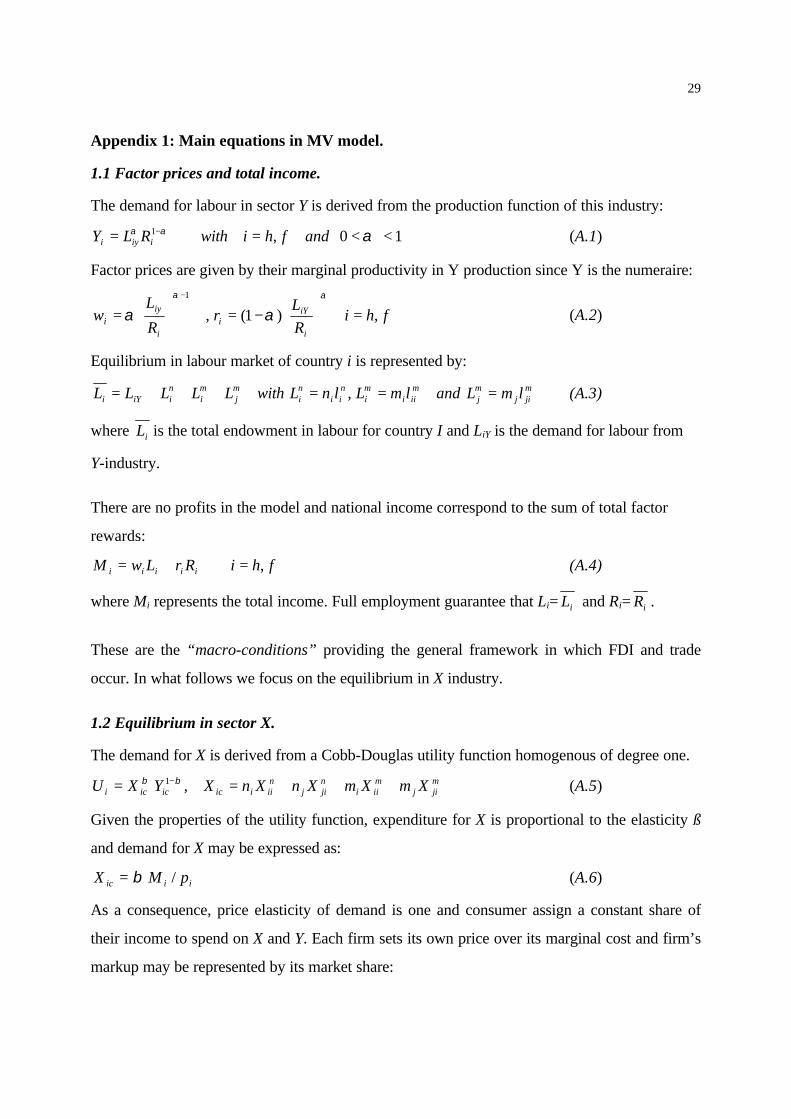
1.1 Factor prices and total income.

The demand for labour in sector Y is derived from the production function of this industry:

10,1 <<== − ααα andfhiwithRLY iiyi (A.1)

Factor prices are given by their marginal productivity in Y production since Y is the numeraire:

fhiR

Lr

R

Lw

i

iYi

i

iyi ,)1(,

1

=

−=

=

− αα

αα (A.2)

Equilibrium in labour market of country i is represented by:

mjij

mj

miii

mi

nii

ni

mj

mi

niiYi lmLandlmLlnLwithLLLLL ===+++= , (A.3)

where iL is the total endowment in labour for country I and LiY is the demand for labour from

Y-industry.

There are no profits in the model and national income correspond to the sum of total factor

rewards:

fhiRrLwM iiiii ,=+= (A.4)

where Mi represents the total income. Full employment guarantee that Li= iL and Ri= iR .

These are the “macro-conditions” providing the general framework in which FDI and trade

occur. In what follows we focus on the equilibrium in X industry.

1.2 Equilibrium in sector X.

The demand for X is derived from a Cobb-Douglas utility function homogenous of degree one.

mjij

miii

njij

niiiicicici XmXmXnXnXYXU +++== − ,1 ββ (A.5)

Given the properties of the utility function, expenditure for X is proportional to the elasticity ß

and demand for X may be expressed as:

iiic pMX /β= (A.6)

As a consequence, price elasticity of demand is one and consumer assign a constant share of

their income to spend on X and Y. Each firm sets its own price over its marginal cost and firm’s

markup may be represented by its market share:

30

fhjiandmnkwithMXpe jkijj

kij ,,,/ === β (A.7)

The term β is the constant share of income spent on X and pj denotes the price of X in country j.

These prices will be identical for firms based in the same country since X is homogenous. But

with positive transport costs and active national firms, prices and quantities differ between i and

j because of higher marginal cost related to export.

The model is completed the model with the assumption that free entry condition drive profits to

zero so that markup revenues cover exactly fixed costs as noted by the following equations:

jiandfhjiwithFGwXepXep inij

nijj

nii

niii ≠=+=+ ,,)( (A.8)

jiandfhjiwithGwFGwXepXep jimij

mijj

mii

miii ≠=++=+ ,,)( (A.9)

Firms in X-industry fix their prices over their marginal cost and pricing equations may be

expressed as:

( ) cwep iniii =−1 (A.10)

( ) )(1 tcwep iniji +=− (A.11)

( ) cwep imiii =−1 (A.12)

( ) cwjep mijj =−1 (A.13)

We do not write equations (A.10)-(A.13) in a complementary-slackness forms since we assume

that right hand side are always positive and that all firms-types exist at the equilibrium with zero

profit.

Equations (A.10)-(A.11) denotes the prices for type-n firms in i and j respectively, while (A.12)

and (A.13) are for type-m firms in i and j.

Replacing (A.7) into (A.10)-(A.13) gives the following expressions for individual outputs:

2i

iii

nii p

cwpMX

−= β (A.14)

2

)(

j

ijj

nij p

tcwpMX

+−= β (A.15)

31

2i

iii

mii p

cwpMX

−= β (A.16)

2j

jjmij p

cwpMjX

−= β (A.17)

32

Appendix 2: Further details concerning MV results.

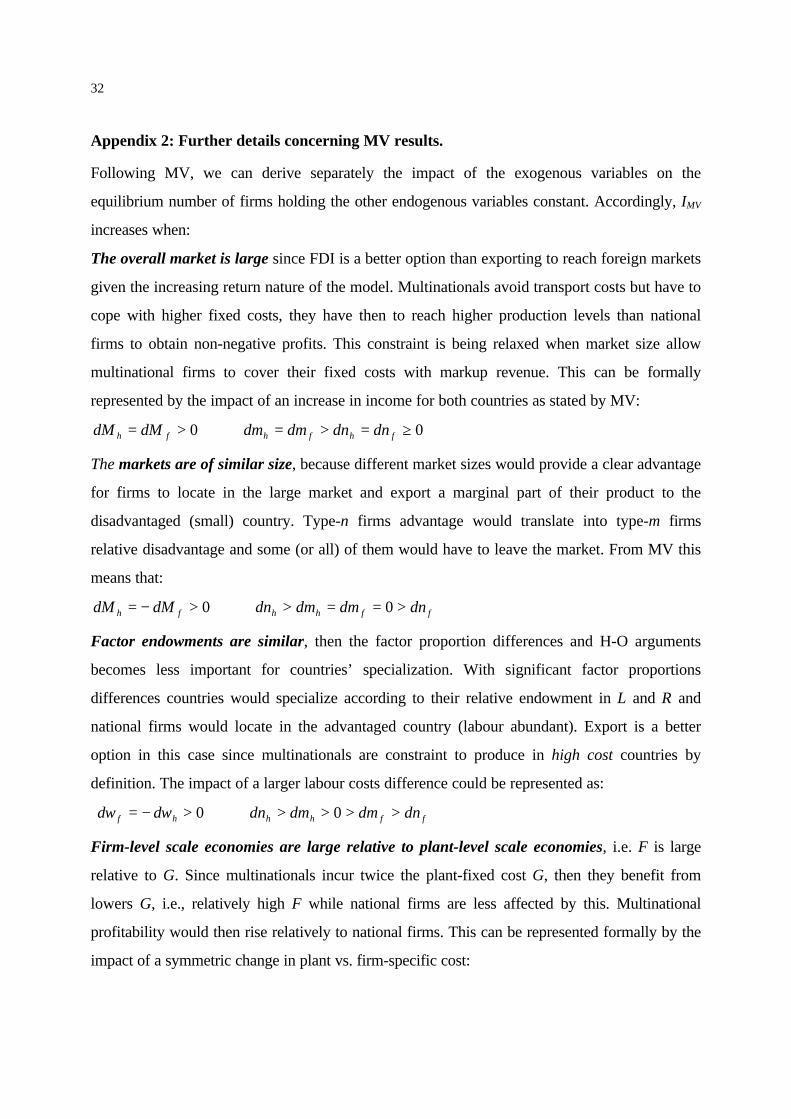
Following MV, we can derive separately the impact of the exogenous variables on the

equilibrium number of firms holding the other endogenous variables constant. Accordingly, IMV

increases when:

The overall market is large since FDI is a better option than exporting to reach foreign markets

given the increasing return nature of the model. Multinationals avoid transport costs but have to

cope with higher fixed costs, they have then to reach higher production levels than national

firms to obtain non-negative profits. This constraint is being relaxed when market size allow

multinational firms to cover their fixed costs with markup revenue. This can be formally

represented by the impact of an increase in income for both countries as stated by MV:

00 ≥=>=⇒>= fhfhfh dndndmdmdMdM

The markets are of similar size, because different market sizes would provide a clear advantage

for firms to locate in the large market and export a marginal part of their product to the

disadvantaged (small) country. Type-n firms advantage would translate into type-m firms

relative disadvantage and some (or all) of them would have to leave the market. From MV this

means that:

ffhhfh dndmdmdndMdM >==>⇒>−= 00

Factor endowments are similar, then the factor proportion differences and H-O arguments

becomes less important for countries’ specialization. With significant factor proportions

differences countries would specialize according to their relative endowment in L and R and

national firms would locate in the advantaged country (labour abundant). Export is a better

option in this case since multinationals are constraint to produce in high cost countries by

definition. The impact of a larger labour costs difference could be represented as:

ffhhhf dndmdmdndwdw >>>>⇒>−= 00

Firm-level scale economies are large relative to plant-level scale economies, i.e. F is large

relative to G. Since multinationals incur twice the plant-fixed cost G, then they benefit from

lowers G, i.e., relatively high F while national firms are less affected by this. Multinational

profitability would then rise relatively to national firms. This can be represented formally by the

impact of a symmetric change in plant vs. firm-specific cost:

33

hffh dndndmdmdGdF =>>=⇒>−= 00

Transport costs are high, in this case export is simply a costly option compared to FDI.

Following MV, we have:

fhfh dndndmdmdt =>==⇒> 00

34

Appendix 3: Definitions of the Variables and data sources:

Variable Description Data SourceYij indicators of bilateral foreign employment,

defined by equations (7), (8) and (9).OECD database: Measuring Globalisation,The role of Multinationals in OECDeconomies, 1999 Edition and StanDatabase, OECD to derive bilateral totalemployment in manufactures.

GDP ln(GDPi)+ln(GDPj), expressed in constantUS dollars 1995

AMECO database, EuropeanCommission- DG ECFIN

ABSGDP abs(GDPi-GDPj), expressed in constantUS dollars 1995

AMECO database, EuropeanCommission- DG ECFIN.

SEND1 abs(SENDi-SENDj); difference in theshare of employment in R&D activityrelative to total employment in the country(*see note below).

OECD Science, Technology and IndustryScoreboard, Benchmarking Knowledgebased economies, OECD 1999, and Standatabase.

SEND2 abs(SENDi-SENDj); difference in thepercentage of students enrolled insecondary school education in the totalpopulation in the country

UNESCO and AMECO database,European Commission- DG ECFIN

CEND abs(CENDi-CENDj); difference in thephysical capital stock per capita

AMECO database, EuropeanCommission- DG ECFIN

RD (R&D Expenditure / Total Employment)i

+ (R&D Expenditure / TotalEmployment)j

Research and Development Expenditure inIndustry (ANBERD), OECD 1999

LANG language dummy variable: 1- samelanguage; 0 - different language

Jon Haveman database available at:http://www.eiit.org/Trade.Resources/TradeData.html

DIST spherical distance between countries’capitals

Jon Haveman database available at:http://www.eiit.org/Trade.Resources/TradeData.html

OPENij )()( jiijij GDPGDPMX ++ , where X and

M are bilateral exports and importsrespectively.

International Trade by CommoditiesStatistics ITCS database, 1988-1997,OECD

* Note:

These numbers have been obtained using per ten thousands number of R&D workers (obtained from theOECD Science, Technology and Industry Scoreboard) and applying this to the total number of employees(obtained from Stan database).

The Centre for Research on Globalisation and Labour Markets was established in the

School of Economics at the University of Nottingham in 1998. Core funding for the

Centre comes from a five-year Programme Grant awarded by the Leverhulme Trust to

the value of almost £1m. The Centre is under the Directorship of Professor David

Greenaway.

The focus of the Centre’s research is economic analysis of the links between changes

in patterns of international trade, cross-border investment and production,

international regulation and labour market outcomes. Researchers in the Centre

undertake both basic scientific and policy-focused research and the Centre supports a

range of dissemination activities.

The School of Economics also publishes Research Papers by the Centre for Research

in Economic Development and International Trade and a Discussion Paper series in

economics. Enquiries concerning copies of the CREDIT papers should be addressed

to Professor Michael Bleaney, CREDIT, School of Economics, University of

Nottingham. Enquiries concerning copies of the Discussion Papers should be

addressed to Professor Richard Disney, School of Economics, University of

Nottingham.

Details on the research papers published by the Centre can be obtained from:

Michelle Haynes

School of EconomicsUniversity of NottinghamNottinghamNG7 2RDUKTel. +44 (0)115 8466447e-mail: [email protected]

Web Site Address:

http://www.nottingham.ac.uk/economics/leverhulme

centre for research on globalisation and labour …

Documents