centralized wind power plant voltage control with optimal power flow algorithm
TRANSCRIPT

Graduate Theses and Dissertations Iowa State University Capstones, Theses andDissertations
2011
Centralized wind power plant voltage control withoptimal power flow algorithmJared Andrew KlineIowa State University
Follow this and additional works at: https://lib.dr.iastate.edu/etd
Part of the Electrical and Computer Engineering Commons
This Thesis is brought to you for free and open access by the Iowa State University Capstones, Theses and Dissertations at Iowa State University DigitalRepository. It has been accepted for inclusion in Graduate Theses and Dissertations by an authorized administrator of Iowa State University DigitalRepository. For more information, please contact [email protected].
Recommended CitationKline, Jared Andrew, "Centralized wind power plant voltage control with optimal power flow algorithm" (2011). Graduate Theses andDissertations. 10335.https://lib.dr.iastate.edu/etd/10335

Centralized wind power plant voltage control with optimal power flow algorithm
by
Jared Andrew Kline
A thesis submitted to the graduate faculty
in partial fulfillment of the requirements for the degree of
MASTER OF SCIENCE
Major: Electrical Engineering
Program of Study Committee: Cheng-Ching Liu, Major Professor
Venkataramana Ajjarapu Manimaran Govindarasu
Iowa State University
Ames, Iowa
2011

ii
Table of Contents
Table of Contents .................................................................................................................... ii!
List of Figures ......................................................................................................................... vi!
List of Tables ......................................................................................................................... vii!
Acknowledgements .............................................................................................................. viii!
Abstract ..................................................................................................................................... x!
Chapter 1 Introduction ...........................................................................................................1!
Chapter 2 Large-Scale Wind Plants and Wind Plant Collection Systems .........................2!
Utility Scale WPPs ...................................................................................................................................... 2!
WTG Characteristics ................................................................................................................................. 2!
Medium-Voltage Collection System ......................................................................................................... 2!
Substation Characteristics ......................................................................................................................... 3!
Chapter 3 The Voltage Control Problem ...............................................................................5!
The Power Flow Equations ........................................................................................................................ 5!
Decoupling of Active and Reactive Power ............................................................................................... 5!
Chapter 4 Optimal VAR Flow Voltage Control for Large Scale Wind Power
Plant .................................................................................................................................8!
Introduction ................................................................................................................................................ 8!

iii
Large-Scale Wind Plants and Wind Plant Collection Systems .............................................................. 8!Medium-Voltage Collection System ....................................................................................................... 8!The Voltage Control Problem ................................................................................................................. 9!Reactive Power Compensation ................................................................................................................ 9!Collection System Losses ...................................................................................................................... 11!
Wind Plant Control .................................................................................................................................. 11!Centralized Control Systems ................................................................................................................. 11!Proposed Approach ............................................................................................................................... 13!Optimal Power Flow .............................................................................................................................. 13!Application to Wind Plant Collection Systems ..................................................................................... 13!
Proposed Control Topology ..................................................................................................................... 14!Control Inputs ........................................................................................................................................ 14!Control Outputs ..................................................................................................................................... 15!Methodology .......................................................................................................................................... 15!Voltage Regulator .................................................................................................................................. 18!Practical Considerations ........................................................................................................................ 18!Physical Implementation ....................................................................................................................... 22!
Conclusion ................................................................................................................................................. 23!
Chapter 5 100 WTG Test System Utilized for Case Study ................................................25!
Test System Model ................................................................................................................................... 25!WTG Data ............................................................................................................................................. 26!Turbine Transformer Data ..................................................................................................................... 27!35kV Cable ............................................................................................................................................ 28!Substation Transformer Data ................................................................................................................. 32!Transmission Line ................................................................................................................................. 34!Reactive Power Resources .................................................................................................................... 34!
Chapter 6 Case Study in WPP Reactive Power Compensation and Centralized
Control Methodologies .................................................................................................35!
Control System Strategies ....................................................................................................................... 35!Optimal Strategy .................................................................................................................................... 35!

iv
Uniform Strategy ................................................................................................................................... 36!Operating Conditions Studied ............................................................................................................... 36!
Cases Studied ............................................................................................................................................ 41!Uniform Dispatch System Limitations .................................................................................................. 42!Optimal Dispatch System Limitations ................................................................................................... 43!
MATPOWER Model ................................................................................................................................ 45!
Results ....................................................................................................................................................... 46!
Chapter 7 Discussion of Results ...........................................................................................49!
System Losses ............................................................................................................................................ 49!
Reactive Power Injections ....................................................................................................................... 49!Normal Conditions ................................................................................................................................ 49!Extreme Conditions ............................................................................................................................... 51!
Voltage Profile .......................................................................................................................................... 53!Normal Conditions ................................................................................................................................ 53!Extreme Conditions ............................................................................................................................... 55!
Cost Effectiveness ..................................................................................................................................... 57!Present Value of Avoided Losses .......................................................................................................... 57!Present Value of Costs of the Proposed Control System ...................................................................... 59!Net Present Value of Proposed Control System .................................................................................... 60!
Significant Assumptions .......................................................................................................................... 60!
Conclusion ................................................................................................................................................. 61!Oportunities for Further Work ............................................................................................................... 62!
References ...............................................................................................................................63!
Appendix 1 Test System Medium Voltage Cable Impedances ..........................................68!
Appendix 2 Case Study Results for “Window” Scenario ...................................................71!

v
Appendix 3 Case Study Results for the “Rectangular” Scenario ......................................72!
Appendix 4 Case Study Results for the “Rectangular” Scenario with Extended
Voltage Range ................................................................................................................76!
Appendix 5 Case Study Results for the “Triangular” Scenario ........................................80!
Appendix 6 Case Study Results for the “Triangular” Scenario with Extended
Voltage Range ................................................................................................................84!

vi
List of Figures
Figure 4-1: Wind plant voltage control. .................................................................................15!
Figure 4-2: OPF flow chart. ...................................................................................................19!
Figure 4-3: OPF flow chart with additional logic to allow fine control. ...............................21!
Figure 5-1: Test collection system one-line diagram. ............................................................25!
Figure 5-2: WTG configuration. .............................................................................................26!
Figure 5-3: Assumed WTG real and reactive power capability. ............................................27!
Figure 6-1: “Triangular” reactive power capability. ..............................................................38!
Figure 6-2: Rectangular reactive power capability requirement. ..........................................39!
Figure 7-1: WTG reactive power injection versus system resistance under normal
conditions utilizing the optimal reactive power dispatch strategy. ..................................50!
Figure 7-2: WTG reactive power injection versus system impedance under extreme
conditions utilizing the optimal dispatch strategy. ..........................................................51!
Figure 7-3: WTG reactive power injection versus system impedance under extreme
conditions utilizing the uniform dispatch strategy. ..........................................................52!
Figure 7-4: WTG 34.5kV bus voltage versus system impedance under normal
conditions utilizing the optimal dispatch strategy. ..........................................................53!
Figure 7-5: WTG 34.5kV bus voltage versus system impedance under normal
conditions utilizing the uniform dispatch strategy. ..........................................................54!
Figure 7-6: WTG 34.5kV bus voltage versus system impedance under extreme
conditions utilizing the optimal dispatch strategy. ..........................................................55!
Figure 7-7: WTG 34.5kV bus voltage versus system impedance under extreme
conditions utilizing the uniform dispatch strategy. ..........................................................56!

vii
List of Tables
Table 5-1: 35kV cable data .....................................................................................................28!
Table 6-2: Summary of operation scenarios studied. .............................................................40!
Table 6-3: Summary of potential real power savings at 100% generation. ...........................46!
Table 6-4: Hours spent per year at each generation level. .....................................................47!
Table 6-5: Estimated annual energy savings. .........................................................................48!
Table 7-1: Comparison between substation resource dispatch strategies. .............................49!
Table 7-2: Summary of voltage profiles created by two reactive power dispatch
strategies under normal conditions. .................................................................................54!
Table 7-3: Summary of bus voltage profiles created by two reactive power strategies
under extreme conditions. ................................................................................................56!
Table 7-4: Summary of loss value scenarios. ........................................................................58!
Table 7-5: Assumed incremental costs of proposed control system. .....................................59!
Table 7-6: Estimated net present value of proposed control system. .....................................60!
Table A1-1: 35kV cable impedances used in test system. .....................................................68!
Table A2-1: Case study results for “window” scenario. ........................................................71!
Table A3-1: Cases study results for “Rectangular” scenario. ................................................72!
Table A4-1: Cases study results for “Rectangular” scenario with extended voltage
range. ................................................................................................................................76!
Table A5-1: Case study results for “Triangular” scenario. ....................................................80!
Table A6-1: Case study results for “Triangular” scenario with extended voltage
range .................................................................................................................................84!

viii
Acknowledgements
There are several people who I would like to thank for their support in completing this
project: The principals at P & E Engineering—D. Blasberg, T. Ernst, R. Kline, and A.
Powers—for teaching me the practical art of power systems design and paying for a
significant portion of my degree; A. Kline, R. Kline, Dr. Liu, and A. Powers for reviewing
drafts of this thesis; Dr. Liu for agreeing to take on an off-campus student and his help with
my research project; and Dr. Ajjarapu and Dr. Govindarasu for agreeing to fill out the
remainder of my committee. Additionally, L. He and N. Acharya provided assistance with
research. Dr. Aliprantis provided assistance with the understanding of Type 4 WTGs. Dr.
McCalley also allowed use of lecture notes from previous semesters.
There are four people without whom I would likely have never gotten to this position.
The first is my wife. It has been very difficult to sit down and spend time on my studies after
long days at work, and her loving support and encouragement has proven very helpful,
especially when I began work on the research and thesis almost two years ago. I would like
to thank her for cooking and doing more than her share of housework while I watched lecture
videos and worked on homework assignments and research.
I have been lucky to have two parents who truly value education. Dad is a Principal
Engineer at P & E Engineering and also spent many years at the companies that became
MidAmerican Energy. Mom is a GT Coordinator with Des Moines Public Schools and has
spent the majority of her career as a classroom teacher. They both genuinely loved and are
very good at their chosen professions. This has spilled over into the career choices of their
children who have followed in their parent’s footsteps. My brother, Dan, is in management
at Xcel Energy in Minneapolis and spent several years as an engineer in transmission
planning. My sister, Kelsey, is a Ph.D. candidate in musicology at Washington University in
St. Louis and hopes to one day teach at the college level.
I have had several excellent teachers through the years, and none has been more
influential than S. Waugh, my high school German teacher. While I was not a poor student
in high school, I did not apply myself to my high school classwork as well as I could have.
With his help and encouragement, I won the Congress-Bundestag scholarship that sent me to

ix
Germany for a year as an exchange student. Without this experience, I doubt that I would
have taken the first few years of college seriously enough to put in the extra hours that were
necessary to excel. I would not be surprised to learn that my academic performance in high
school was in the bottom half of the freshman engineering students with whom I started my
career at Iowa State, but my performance as an undergraduate student was significantly better
than average. While many people, including J. Otto, E. Pilartz, H. Prüßmann, and the Nagel
and Wippenhohn families (especially P. Nagel and E. Wippenhohn) helped to make the
experience a positive one, it would not have happened without Herr Waugh.

x
Abstract
This thesis presents a method of controlling the reactive power injected into a medium-
voltage collection system by multiple wind turbine generators such that the voltage at one
bus is maintained at a specified level. The proposed control accounts for the system
impedance between the wind turbine generator terminals and the point of interconnect, and
utilizes an optimal power flow algorithm to dispatch reactive power amongst the wind
turbine generators. This optimal power flow algorithm minimizes real power losses within
the wind power plant and avoids operating conditions that violate various operating
constraints.
This thesis presents a 100 wind turbine generator wind plant test system and uses this
test system to demonstrate the potential increased revenues occasioned by the proposed
control system as compared to a system that dispatches the wind turbine generator reactive
power injections uniformly. Analysis shows that it can be cost effective to install the
proposed control system.

1
Chapter 1 Introduction
The rapid growth of the wind industry in the United States and elsewhere has forced
large wind power plants (WPPs) to provide ancillary services more similar to what is
expected of a traditional power plant. To meet this demand, wind turbine generator (WTG)
manufacturers offer centralized control systems that can provide many of these services [1].
This thesis focuses on one of these ancillary services, voltage and/or reactive power
control; however, the control proposed could be expanded to other ancillary services such as
frequency regulation. Chapter 2 provides an introduction to the topology of large-scale wind
power plants. The standard AC power flow equations are provided in Chapter 3 along with
their implications for voltage control. A centralized voltage control algorithm is proposed in
Chapter 4.
The remainder of the thesis focuses on the benefits of the proposed control system,
namely the ability to minimize electrical losses within the WPP and the ability to avoid
violating system constraints. Chapter 5 presents a test WPP system that is used in the case
study discussed in Chapter 6 and attempts to estimate the reduction in collection system
energy losses caused by the use of an optimal reactive power dispatch strategy. The results
of the case study are discussed in Chapter 7.
In the remainder of this paper, equations enclosed in a box are direct quotes from the
source named in text.

2
Chapter 2 Large-Scale Wind Plants and Wind Plant Collection Systems
Utility Scale WPPs
For the purposes of this paper, utility-scale WPPs consist of several wind turbines that
are connected to the bulk transmission system at one point. The following is a general
description of the utility scale WPPs that are presently being built in the United States. The
IEEE PES Wind Plant Collector System Design Working Group has published several papers
on the subject of collection system design including [1]–[9].
WTG Characteristics
In large-scale WPPs, the individual wind turbine generators (WTGs) typically have
terminal voltages in the low-voltage spectrum. Figure 1 in [2] shows a turbine with a 575V
turbine terminal voltage and Figure 1 in [3] states that terminal voltages between 400V and
690V are typical. The individual wind turbines are connected to a medium voltage collection
system via a transformer [2]. This transformer may be a part of the turbine itself or a
separate unit located outside the tower [3]. Where the transformer is located outside the
WTG, it is typically a three-phase pad-mounted transformer similar to those utilized on
utility distribution systems [2].
Medium-Voltage Collection System
The medium-voltage collection systems utilized in WPPs is discussed in [2] and [4].
Distribution class components in the 15kV, 25kV, and 35kV classes are widely available for
both underground and overhead distribution systems. These components are defined by
industry standards such as [10], [11], [12], and [13]. The use of higher voltages has several
well-documented advantages, including reduced losses, ability to carry larger amounts of
power over longer distances, and better voltage performance.
The typical medium voltage collection system at WPPs constructed in the United States
is operated at 34.5kV [2]. While [2] does not justify the use of 34.5kV as the standard
collection system voltage; it appears to be that this is the highest voltage class for which

3
standard distribution system components, especially cable accessories such as splices,
terminators, and elbows, are available is 35kV.
The use of standard medium-voltage components is typical of utility practices. Use of
standard components minimizes inventory and increases familiarity of crews with correct
installation practices reducing the probability of serious mistakes during installation [4].
Though not specifically discussed in [4], use of standard components reduces costs due to the
widespread availability of the components (Reference [2] describes pad-mounted
transformers as “commodities”) and provides for some interchangeability between
manufacturers. These standard utility practices have carried over to the wind industry and
WPP medium voltage collection systems are typically constructed with standard distribution
class components [4].
The medium-voltage collection systems can be overhead, but are more typically
underground as they are more acceptable to landowners and can also result in reduced losses,
higher reliability, and fewer restrictions on the movement of construction equipment. These
collection circuits are typically constructed in a radial fashion with the turbines connected in
a daisy chain, utilizing junction boxes and the loop-feed bushings in the turbine transformers
[2].
In the author’s experience, this radial configuration is significantly different than what
is typical of modern underground residential distribution (URD) circuits. While practices
vary between utilities, in a typical URD circuit the underground cable would be configured in
a loop with a normally open point in the middle. This allows any individual cable segment to
be de-energized and repaired while maintaining service to customers and allows service to
customers to be restored prior to repairing a failed cable. This method reduces outage
durations, but results in a higher installation cost. In a looped system, the cables will also
necessarily be normally operated at significantly less than maximum capacity, significantly
reducing losses.
Substation Characteristics
The medium voltage collection circuits terminate in a substation and are connected to
the main substation bus via circuit breakers. These circuit breakers and main bus are

4
typically an open bus design [6]. The alternative to an open bus design is metal-clad
switchgear, which the author has also seen on recent projects.
Each collector circuit may be connected to a circuit breaker that is dedicated to that
cable, or multiple cables may be combined and connected to one circuit breaker. The
collection circuits are then connected to the bulk transmission system via transformers in the
substation and a transmission line. This transmission line may amount to bus across a fence
into an adjacent switchyard or may be several miles long, depending on the distance to the
point of interconnect [2]. Depending on a variety of factors, the WPP substation may contain
one or more transformers [9].
The substation may also contain reactive power compensation equipment [1].

5
Chapter 3 The Voltage Control Problem
Reactive power is commonly used to control voltages on power systems. The
justification for using reactive power to control voltage is described in several standard
power systems analysis textbooks and other resources, including [14] and [15].
The Power Flow Equations
One form of the power flow equations are given in (3.1) and (3.2), which are given as
Equation (10.5) in [14] (p. 326) and Equations (25a) and (25b) in [15].
Pi = Vi Vk Gik cosθik +Bik sinθik( )k=1
n
∑ (3.1)
Qi = Vi Vk Gik sinθik −Bik cosθik( )k=1
n
∑ (3.2)
Where:
• Pi is the net real power injection at bus i
• Qi is the net reactive power injection at bus i
• |Vi| is the magnitude of the voltage at bus i
• |Vk| is the magnitude of the voltage at bus k
• Gik is the real component of the entry at position i, k of the bus admittance
matrix YBUS [15]
• Bik is the imaginary component of the entry at position i, k of the bus admittance
matrix YBUS [15]
• θik is the angular difference between the complex voltages of buses i and k
Decoupling of Active and Reactive Power
The decoupling of active and reactive power is discussed in [14] and briefly in [17]. In
[14], the decoupling of active and reactive power is demonstrated by developing the power
flow problem, the Newton-Raphson solution algorithm, and the Jacobian. Here, a less
rigorous approach is utilized to arrive at the same conclusion.

6
To demonstrate the decoupling of active (real) and reactive power, take the partial
derivative of (3.1) and (3.2) with respect to θk and Vk. This yields (3.3), (3.4), (3.5), and
(3.6) which are given as Equation (10.40) in [14] (p. 345) and (9), (11), (13), and (15) in [16]
(p. 10) with the p and q subscripts replaced with i and k, respectively.
∂Pi∂θk
= Vi Vk Gik sinθik −Bik cosθik( ) (3.3)
∂Pi∂Vk
= Vi Gik cosθik +Bik sinθik( ) (3.4)
∂Qi
∂θk= − Vi Vk Gik cosθik +Bik sinθik( ) (3.5)
∂Qi
∂Vk= Vi Gik sinθik −Bik cosθik( ) (3.6)
In typical overhead transmission systems, the resistance and θik will be relatively low
[14]. Additionally, voltages will be close to 1.0 pu under most operating conditions.
Assume:
θik ≈ 0
Vi ≈1
Vk ≈1
Gik ≈ 0
Substituting these into (3.3), (3.4), (3.5), and (3.6) yields (3.7), (3.8), (3.9), and (3.10).
∂Pi∂θk
≈ −Bik (3.7)
∂Pi∂Vk
≈ 0 (3.8)
∂Qi
∂θk≈ 0 (3.9)

7
∂Qi
∂Vk≈ −Bik (3.10)
Equation (3.8) implies that an incremental change in real power injection at a particular
bus has relatively little impact on bus voltage at neighboring buses. Similarly, (3.9) implies
that an incremental change in the reactive power injection at a particular bus will have
relatively limited impact on the angular difference across the branches connected to that bus.
Equation (3.7) implies that an incremental change in the real power injection at a
particular bus will have a relatively large impact on the angular difference across the
branches connected to that bus. Similarly, (3.10) implies that an incremental change in the
reactive power injection at a particular bus will have a relatively large impact on voltage at
neighboring buses.
Stated differently, real and reactive power control different properties. On a steady-
state basis, changes to the real power injections can best control the angular difference across
a branch. Similarly, changes to the reactive power injections control bus voltages [14].

8
Chapter 4 Optimal VAR Flow Voltage Control for Large Scale Wind
Power Plant
Introduction
The wind industry in the United States has grown rapidly over the past several years.
Installed wind capacity in the United States totaled 40 181 MW at the end of 2010. Of these,
5 116 MW were added in 2010 [18]. The growth of the wind industry has forced large wind
plants to provide ancillary services similar to those provided by conventional generation
facilities. In order to provide these ancillary services, wind turbine generator (WTG)
manufacturers offer centralized control systems [1].
Large-Scale Wind Plants and Wind Plant Collection Systems
For the purposes of this paper, large utility-scale wind power plants (WPPs) consist of
several WTGs that are connected to the bulk transmission system at one point. References
[1] through [9] were prepared by the IEEE PES Wind Plant Collector System Design
Working Group and describe the general topology and design considerations of the wind
plants currently being constructed in the United States.
Medium-Voltage Collection System
The individual WTGs utilized on recent utility scale projects in North America tend to
have nameplate generation capabilities between 1.5 and 2.5 MW. The WTGs in use on
utility scale WPPs generally have terminal voltages between 400V and 690V [3]. In the
author’s experience, 690V is a very common terminal voltage. The individual WTGs are
connected to a medium-voltage collection system through a transformer located within or
next to the WTG [3]. If the transformer is located outside of the WTG, the transformer is
likely to be very similar to the three-phase pad-mounted transformers utilized on utility
distribution systems. The medium-voltage collection systems are typically operated with a
nominal voltage of 34.5kV [2].
The medium-voltage collection system connects the individual WTGs with a substation
that contains a transformer connecting the medium-voltage collection system with the bulk

9
transmission system. The medium-voltage collection system is normally constructed in a
radial topology with underground cables, though overhead collection systems have also been
constructed [2].
The Voltage Control Problem
Reactive power is commonly used to control voltages on power systems. The
justification for using reactive power to control voltage is described in several standard
power systems analysis textbooks including [14]. In typical overhead transmission systems,
the resistance will be small compared to the reactance. On a steady state basis, the result of
this is that bus voltages are best controlled by changing the reactive power injections while
the difference in voltage angle between buses is best controlled by changing the real power
injections [14].
Reactive Power Compensation
A large wind plant can consist of many WTGs, which may have reactive power
capability, and the WPP may possess substation reactive power resources such as switched
capacitors and reactors or dynamic devices such as static VAR compensators [1]. There have
been several papers discussing the use of wind plants for the control or support of voltages on
the bulk transmission system including [19] and [20] and discussion of the WTG
characteristics, including reactive power capability, particularly the doubly fed induction
generators (DFIG) including [5], [19], and [21]. Reference [22] proposes a transient model
of the DFIG for use in transmission system level studies.
Reference [1] discusses the requirements and design methodology for WPP reactive
power compensation systems in the United States subject to regulation by FERC. This
paragraph is a summary of this discussion. The interconnecting utility (transmission
provider) performs a system impact study as a part of the interconnection process. FERC
Order 661-A [23] allows the interconnecting utility to require the WPP to supply reactive
power sufficient to provide a power factor between 0.95 leading and 0.95 lagging if the
system impact study shows that it is necessary to maintain system reliability. This reactive
power requirement typically applies to the complex power flow at the point of interconnect.
The Large Generator Interconnection Agreement lays out other reactive power requirements

10
that the WPP is expected to meet. The WPP is required to install sufficient reactive power
resources (either WTGs with reactive power capability, substation resources, or a
combination of the two) to meet this power factor requirement. If needed for reliability
reasons, the interconnecting utility may also require that the reactive power resources be
“dynamic” to provide continuous smooth control of the interconnect bus voltage. The WPP
may be required to meet the reactive power requirement may be at one specific voltage, or
over a range of voltages [1]. While not discussed in [1], reactive power requirements in the
ERCOT region are different [24].
WTG Reactive Power Capability
The reactive power capabilities of the common WTG designs are discussed in [5].
References [19] and [21] also provide discussion of the capabilities of Type 3 (DFIG) WTGs.
Type 1 and 2 designs (induction generators) are generally not capable of providing reactive
power compensation, and the machines themselves actually absorb reactive power.
Manufacturers of Type 1 and 2 designs normally provide several stages of switched power
factor correction capacitors. Type 3 and 4 (full converter) WTGS are capable of operating as
dynamic reactive power resources and may also be capable of generating reactive power
when the WTG is not producing real power. The capability of Type 4 WTGs may vary with
terminal voltage [5].
Substation Reactive Power Resources
If the WTGs do not have sufficient capability to meet the interconnect requirements
described above, reactive power resources must be provided in the substation. These
resources may include switched capacitors and reactors, static VAR compensators (SVC), or
static synchronous compensators (STATCOM). STATCOMs and SVCs can operate as
dynamic resources, but are more expensive than fixed capacitors and reactors. If the
transmission provider requires that the plant be capable of providing smooth voltage control,
a combination of DFIG WTGs and switched capacitors and reactors may be acceptable [1].
Reference [1] also discusses low-voltage ride-through requirements and the role that
power factor compensation has in low-voltage ride-through requirements.

11
Collection System Losses
Energy that is generated by the WTGs but not delivered to the point of interconnect
reduces the operator’s potential profits [9]. The analysis of losses in the WPP is discussed in
detail in [6]. Additionally, losses in specific pieces of equipment are discussed in [4] and [9].
Energy can be lost through electrical resistance in the system and no load losses in
transformers. Furthermore, energy that is not generated due to equipment failures within the
WPP should also be considered as a portion of system losses. A thorough collection system
design will be based on total life-cycle cost. This analysis will determine if the incremental
savings in losses occasioned by a design change offset the cost of that design change [6].
In addition to their consideration during the design phase, losses should be a
consideration during the operation of the WPP as well [25], [26].
Wind Plant Control
Centralized Control Systems
Reference [1] alludes to centralized control systems that can provide ancillary services
that are required by transmission providers. Reference [27] describes the features that are
available with the control systems from one manufacturer. In addition to other features, these
control systems can monitor voltage and current at the substation and adjust the reactive
various power resources (including the WTGs) to meet a desired voltage set point.
The remainder of this paper assumes that the wind plants will typically regulate voltage
at a specified point in the system. There are several means of allocating the reactive power
that is injected by the turbines amongst the several turbines. The simplest would be to divide
the total amount to be supplied equally amongst the WTGs. References [28], [29], and [30]
propose methods of dispatching reactive power proportionally amongst the individual WTGs
based on the relative reactive power capability of each WTG. This has the advantage of
maintaining an equal margin between the turbine operating point and the maximum possible
injection [28]. Reference [31] provides a method for using a central proportional integral
control to regulate the reactive power flow at the point of interconnect, but provides each
WTG with the same power factor signal. The methods presented in [28], [29], [30], and [31]

12
have the advantage of being relatively simple to implement but appear to ignore the
differences in impedance between the WTG terminals and the point of interconnect across
the WPP.
Reference [32] proposes a method dispatching reactive power in a large WPP that
regulates voltage at a pre-determined location and considers the impedance of the collection
system in allocating reactive power amongst the WTGs.
Other papers also present methods of dispatching reactive power but focus mostly on
low voltage ride through. These include [33] and [34].
References [25] and [26] propose dispatching reactive power in an offshore WPP
utilizing a particle swarm optimization method. The WPP referenced in these papers is
connected to the mainland 400kV transmission system via submarine 150kV AC power
cables. While these papers develop the general OPF problem that is broadly applicable to
many WPPs with AC collection systems, and advocate use of an OPF algorithm to dispatch
reactive power during the planning and operations stage, they do not extend the concept to
the development of the reactive power dispatch to a controller that is intended for use in an
on-line environment to regulate voltage at a specific bus.
Reference [35] presents a centralized control scheme that dispatches reactive power
amongst the WTGs using an optimal power flow algorithm. Though [35] briefly discusses
using the WPP to control interconnect bus voltage, the proposed control system receives the
desired reactive power injection from the transmission operator. The control system appears
to be open loop and does not contain a feedback loop to regulate the WPP reactive power
injection to the desired level.
This paper presents an optimal control system similar to [25], [26], and [35] but applied
to the large-scale WPPs currently being constructed in the United States. The control system
contains a feedback loop and is capable of being used in an on-line environment to regulate
voltage to a predetermined set-point.

13
Proposed Approach
The approach proposed in this paper is to allocate the reactive power amongst the
WTGs and substation resources using an AC optimal power flow algorithm. This has the
advantage of minimizing losses and can also incorporate the substation VAR resources.
Optimal Power Flow
Optimal power flow is an extension of the economic dispatch problem in which the
constraints include the set of power flow equations describing the transmission system. In
the classic optimal power flow problem, the generation dispatch of a power system is
determined so as to find the dispatch that will satisfy the system load at the lowest cost. It is
also possible to minimize losses in the system or the amount of load to be shed [36].
By including constraints such as minimum and maximum bus potentials, branch
currents, and generator real and reactive power injections, the optimal power flow solution
can be forced to realize the various constraints on the operation of the system. Some of the
possible control variables include generator real power injection and terminal voltage,
transformer load tap changer (LTC) position (where present), and capacitor switch status.
The system model would need to include the loads at each bus, branch impedances, generator
incremental cost data and constraints. Constraints on the solution would typically include
transmission line flows, bus voltages, and generator minimum and maximum real and
reactive power injections [36].
Application to Wind Plant Collection Systems
In the operation of the in-plant electrical system of a WPP, the problem is substantially
different. The objective of site operation is obviously to maximize profits which are
determined by the real power delivered to the transmission system at the point of
interconnect and therefore requires the minimization of losses within the WPP. Under
normal operating conditions, the WTG real power injections are determined by the wind
prevailing at each WTG. The only way to maximize the real power delivered to the point of
interconnect is to minimize the real power losses within the site. Because the ability to
control generator real power injections has been taken away, the only means to reduce

14
system losses is to change the reactive power dispatch. As described above, the WPP is often
required to regulate voltage at a predetermined bus to a specific level. This serves as a
further constraint on the reactive power dispatch.
In the case of a WPP, the control variables include the WTG reactive power injection
(assuming that the turbines have means of varying the reactive power injection), and may
include the transformer LTC tap position (the substation transformers are often not supplied
with load tap changers and [9] recommends avoiding them), switched capacitor status, and
the reactive power injection from a static VAR compensation system. The system model
would need to include all branch impedances including cables, overhead lines, and
transformers. The transformers and medium-voltage cable systems are generally designed to
carry the maximum expected load, thus thermal constraints are typically not a limiting
condition. Constraints include bus voltages, generator minimum and maximum reactive
power injection, and, if applicable, maximum and minimum transformer LTC position.
The discussion of the optimal power flow problem provided in the paragraphs above is
consistent with [25], [26], and [35], except that load tap changers appear to be common in the
systems described in [25] and [26].
Proposed Control Topology
The proposed control system will regulate the voltage or reactive power flow at a
designated point in the system (usually the point of interconnect) to a predetermined value
while dispatching the reactive power amongst multiple wind turbines so as to minimize total
system losses. The inputs and outputs of the proposed control are listed below. This
generally agrees with the formulations provided in [25], [26], and [35].
Control Inputs
• System data (branch impedances, branch shunt admittances, transformer taps,
etc.)
• Status of substation reactive power resources
• Limitations on changes to substation reactive resources
• Equipment thermal limitations
15
• Bus voltage limitations
• WTG real power injections
• Voltage set point and regulated bus
• WTG reactive power capabilities
• Real power production at each WTG
Control Outputs
• Reactive power injected by each WTG
• Changes to status of substation reactive power resources
Methodology
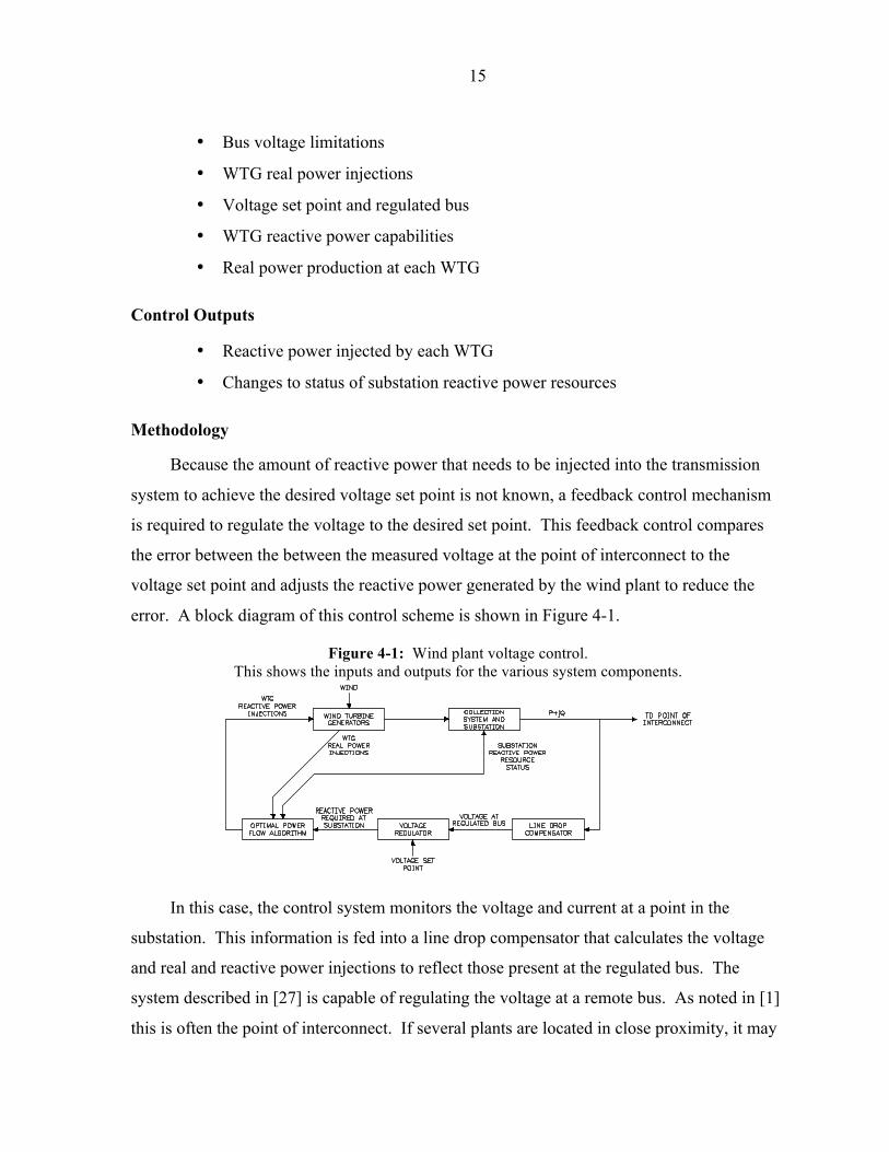
Because the amount of reactive power that needs to be injected into the transmission
system to achieve the desired voltage set point is not known, a feedback control mechanism
is required to regulate the voltage to the desired set point. This feedback control compares
the error between the between the measured voltage at the point of interconnect to the
voltage set point and adjusts the reactive power generated by the wind plant to reduce the
error. A block diagram of this control scheme is shown in Figure 4-1.
Figure 4-1: Wind plant voltage control. This shows the inputs and outputs for the various system components.
In this case, the control system monitors the voltage and current at a point in the
substation. This information is fed into a line drop compensator that calculates the voltage
and real and reactive power injections to reflect those present at the regulated bus. The
system described in [27] is capable of regulating the voltage at a remote bus. As noted in [1]
this is often the point of interconnect. If several plants are located in close proximity, it may

16
be necessary to regulate a different bus or even a fictitious point within the plant. This has
the effect of creating “voltage droop” and allows the plants to share voltage regulation duties
[37]. The calculated voltage at the regulated bus is fed into the voltage regulator which
compares the measured voltage with the voltage set point and calculates the reactive power
that the OPF should deliver to the substation in order to produce the desired voltage.
In order to solve the OPF, the algorithm will also need the real power injected by each
WTG, the voltage limits at each bus, and the current or MVA limits in each branch. It is
assumed that under normal conditions the real power injected by each WTG will be
determined by prevailing wind conditions and the WTG real power injections would be
equality constraints. If generation is curtailed due to transmission constraints or the wind
plant is providing frequency regulation, this would not be the case. The OPF also needs to
know the status of the substation VAR resources. For switched shunt devices such as
capacitors and reactors, the number of times that the devices are switched should be limited
to avoid excessive wear and to reduce circuit breaker or circuit switcher maintenance costs.
Additionally, a delay must be built in to prevent reenergizing a capacitor until the voltage
across the capacitor has decayed to a point where the energizing transients will be acceptable
[38]. The optimal power flow problem is developed below.
minPloss = Iik2 Rik
ik=1
n
∑ (4.1)
For all n branches
Subject to:
Pi = Vi Vk Gik cosθik +Bik sinθik( )k=1
n
∑ (4.2)
Qi = Vi Vk Gik sinθik −Bik cosθik( )k=1
n
∑ (4.3)
PGi = PWINDi (4.4)
VPOI = VSETPOINT (4.5)
QPOI =QVREG (4.6)

17
QMINWTGi ≤QWTGi ≤QMAXWTGi (4.7)
VMINi ≤ Vk ≤ VMAXi (4.8)
Sik ≤ SMAXik (4.9)
Where:
• PGi is the real power injected at bus i
• PWINDi is the real power that the WTG at bus i is capable of injecting based on
prevailing wind conditions
• QPOI is the reactive power supplied to the point of interconnect
• QVREG is the reactive power demanded by the voltage regulator
• |VPOI| is the voltage magnitude at the point of interconnect (or other regulated
bus)
• |VSETPOINT| is the scheduled voltage at the point of interconnect
• QMINWTGi is the maximum reactive power that the WTG at bus i can absorb
• QWTGi is the reactive power supplied by the WTG at bus i
• QMAXWTGi is the maximum reactive power that the WTG at bus i can supply
• |VMINi| is the minimum voltage magnitude each bus i
• |Vi| is the voltage magnitude at bus i
• |VMAXi| is the maximum voltage magnitude at bus i
• |Sik| is the apparent power flowing in branch ik
• |SMAXik| is the maximum apparent power flow in branch ik
• |Iik| is the current magnitude flowing in branch ik
• Rik is the positive sequence AC resistance in branch ik
• Gik and Bik are the real and imaginary components of the bus admittance matrix
Note that (4.2) and (4.3) are given as Equation (10.5) in [14] (p. 326). The formulation
of the optimal power flow problem given in (4.1)–(4.9) is consistent with the formulation
provided in [25], [26], and [35].

18
Voltage Regulator
There are numerous possible topologies that would be suitable for the voltage regulator.
Proportional integral derivative (PID) controllers are commonly used in industry for a variety
of functions [39]. The author sees no reason why they could not be adapted to this purpose.
A transfer function for a standard PID controller is provided in Equation (12.57) in [39] (p.
601), which is repeated in (4.10) below.
GPIDapp s( ) = KP +Ki
1s+Kd
sτ s+1
(4.10)
The constants Kp, Ki, and Kd are selected based on desired control response [39].
Practical Considerations
Dead Band and Coarse Control
A dead band would likely be implemented as a part of the voltage regulator. This
would mean that the control system would solve the OPF only after the measured voltage
deviated from the set point by more than a predetermined amount for a specified duration.
The width of the dead band would be based on discussions with the transmission provider
and the delay would be long enough that the control would not act for faults or other
temporary conditions. This would serve to reduce the computational requirements while still
ensuring that voltage is adequately regulated. Additionally, it would likely be desirable to
solve the OPF at regular intervals or after large changes in real power to ensure that the
reactive power resources are still dispatched optimally. A flow chart showing the logic that
will initiate an OPF solution is provided in Figure 4-2.
Fine Control
This dead band will cause the control system to provide a relatively coarse regulation of
the desired set point. Two possibilities exist if fine voltage control is necessary. The first
possibility is to use dynamic substation reactive power resources such as static VAR
compensators. The alternative is to adjust the WTG reactive power injections as necessary
using linear sensitivity analysis of the OPF results.

19
Figure 4-2: OPF flow chart. This shows the logic used in executing the OPF.
Linear sensitivity analysis is discussed briefly in [40] in the context of linearizing the
power flow equations. This method utilizes partial derivatives to show the variation in one
quantity when another quantity is changed. This method is only useful for small deviations
from the original power flow solution. This is especially true in cases where the sensitivity
factor is for voltage or reactive power flow [40].
In this case, the OPF solution is linearized. One sensitivity coefficient is calculated for
each WTG and shows the change in reactive power injection at the WTG for a change in
reactive power delivered to the point of interconnect. An inelegant way of approximating the
linear sensitivity coefficients is to solve the OPF twice, once with the reactive power
demanded by the voltage controller, and the second with a small incremental change. The

20
linear sensitivity coefficients are then calculated by comparing the reactive power dispatches
from the two OPF solutions.
The linear sensitivity coefficient for WTG i, δ QWTGi, is defined in (4.11). This
provides the sensitivity of the reactive power injected by WTG i to changes in reactive power
provided to the bulk transmission system at the point of interconnect.
δQWTGi =∂QWTGi
∂QPOI
≈ΔQWTGi
ΔQPOI
(4.11)
Where:
• QWTGi is the reactive power injected by WTG i
• QPOI is the reactive power injected at the point of interconnect
Define ∆QPOI as the change in power delivered to the bulk transmission system using
(4.12).
ΔQPOI =QNEWPOI −QPOI (4.12)
Where:
• QNEWPOI is the new reactive power delivered to the bulk transmission system at
the point of interconnect
• QPOI is the reactive power delivered to the point of interconnect in the OPF
solution
Next define the change in reactive power generation at WTG i, ∆QWTGi, using (4.13).
ΔQWTGi = δWTGi •ΔQPOI (4.13)
Next define the new reactive power generation at WTG i, QNEWWTGi, using (4.14).
QNEWWTGi =QPOI +ΔQPOI (4.14)
Where QPOI is the reactive power injection at WTG i from the OPF solution.
It is possible that changing the reactive power injections in this manner may cause the
bus voltages at one or more buses to violate constraints. The fine control should be used for
relatively small adjustments that have negligible impact on voltage constraints. The
difference between the actual reactive power being delivered to the point of interconnect and

21
the value used in the last OPF solution would be used as a trigger to run a new OPF solution.
This logic is shown in Figure 4-3.
Figure 4-3: OPF flow chart with additional logic to allow fine control.

22
Operation at Extreme Voltages or Reactive Power Injections
It is also important to note that the OPF algorithm will fail to return a feasible solution
if it is unable to deliver the desired reactive power without violating constraints. This can be
handled in two ways. The first is to limit the amount of reactive power that the voltage
regulator can demand. The disadvantage to this is that the maximum reactive power that the
WPP can deliver (or absorb) is dependent on the voltage at the point of interconnect. As an
example, analysis shows that in situations where the WPP substation transformer is not
equipped with a load tap changer, the POI bus voltage is high, and the WPP is being asked to
supply large amounts of reactive power, the voltages at the electrically remote WTG buses
will reach high levels and the remote WTGs may begin to absorb reactive power. This keeps
the bus voltage at that WTG within limits, but reduces the reactive power that can be
delivered and increases losses. At moderate voltage levels this is unlikely to happen unless
the collection circuits are very long. See Chapter 7 for more discussion of this issue.
Another option is to implement logic that executes the OPF again if it fails. For the
second attempt, the algorithm would be reconfigured so that it maximizes the reactive power
that the WPP absorbs or delivers to the transmission system without reducing the real power
generated by the WTGs. This would likely result in increased losses, but would allow for the
WPP’s full reactive power capacity to be utilized without exceeding equipment limitations.
This would transform (4.1) into (4.15) or (4.16) below. All constraints remain identical to
those above, which have not been repeated for brevity.
maxQPOI (4.15)
or:
minQPOI (4.16)
Where QPOI is the reactive power injected into the transmission system at the point of
interconnect.
Physical Implementation
The centralized control proposed in this article would be located at the WPP. The
control can be located in the substation control building or, alternatively, in the WPP

23
operations building with transducers or metering equipment located in the substation control
building measuring the voltage, current, and real and reactive power. The WPP SCADA
system would provide these measurements to the control system. In the author’s experience,
fiber optic communications networks are typically built alongside the medium-voltage
collection systems at large-scale WPPs. These fiber optic networks connect the WTGs with
the plant SCADA system and can be used to communicate the reactive power dispatch to the
individual WTGs. The local controllers at the individual WTGs would then be responsible
for making adjustments to produce the desired level of reactive power.
The transmission provider can provide the voltage set point in a number of ways. In
many cases, the transmission provider already has an existing SCADA connection with the
WPP. The voltage set point can be provided via this SCADA link. Otherwise, voltage
schedules can be provided in advance and entered into the SCADA system by WPP
personnel.
As the majority of the SCADA equipment necessary to implement the control is already
present in the majority of cases, the additional cost to implement this control would be
largely limited to the cost of implementing the OPF software and the servers necessary to
handle the extra computing load.
Conclusion
The control system described in this paper presents a method of distributing reactive
power amongst the WTGs and other reactive power resources that minimizes system losses
while regulating voltage at one point in the system. It is also capable of integrating voltage
constraints that exist on the WPP collection system and avoiding operating conditions that
violate these constraints.
There are several opportunities for further work. Perhaps the most obvious is the
integration of such a reactive power dispatch scheme into a commercial WPP control system.
Reference [27] discusses several ancillary services that commercial WPP control systems are
capable of providing. These include frequency response and generation curtailment.
Frequency response and generation curtailment necessarily require reducing the real power
generation below the level that the prevailing wind is capable of producing, this is especially

24
true if the WPP is expected to respond to under-frequency events [27]. The optimal reactive
power dispatch could be extended to the real power dispatch under conditions when the real
power generation is curtailed so that the WPP can respond to under-frequency events.

25
Chapter 5 100 WTG Test System Utilized for Case Study
Test System Model
Figure 5-1: Test collection system one-line diagram.
A 100-1.5 MW (150 MW total) WTG test system model was created using the
MATPOWER software package. The MATPOWER AC OPF function utilizes a primal-dual
interior point algorithm by default [41]. The software package also has a standard AC load
flow algorithm. This model uses data that the author believes to be typical of WPPs
currently under construction in the United States. The model assumes 1.5 MW WTGs with
nominal terminal voltages of 690V. The WTGs are connected to an underground 34.5kV
collection system using pad-mounted transformers. The 34.5kV collection system feeds into

26
a substation with five 38kV circuit breakers. This substation is connected to a 138kV bulk
transmission system via a transformer. The use of 1.5 MW WTGs with a terminal voltage of
690V is consistent with [42]. The use of pad-mounted transformers at each WTG is
consistent with [2]. The use of a 34.5kV medium voltage collection system is consistent with
[2]. In many parts of the United States, 138kV is a common bulk transmission voltage [43].
The system impedances are discussed in the paragraphs that follow. This model is
positive sequence only, as the intention is only to run balanced three-phase load flow and
OPF simulations. A one-line diagram of the system is shown in Figure 5-1. The discussion
of system grounding, while interesting and important, is outside of the scope of this paper.
Due to space limitations, the WTGs are simplified in Figure 5-1. Each WTG is
assumed to have the basic layout shown in Figure 5-2.
Figure 5-2: WTG configuration. The WTG connects to the medium-voltage collection system through a transformer.
Note the loop feed bushings allowing convenient daisy chaining of WTGs.
WTG Data
The WTGs are assumed to be 1.5 MW Type 3 doubly fed induction generators (DFIG).
Each is assumed to be capable of supplying or absorbing 726kVAR from minimum to full
generation. It is assumed that when the WTG is not generating real power, it will be capable
of producing or absorbing 200kVAR as described in [42]. This is shown in Figure 5-3. It is
important to note that several references including [19] and [21] show that the reactive power

27
capability of Type 3 (DFIG) WTGs increases as real power generation decreases. The
assumed reactive power capability used in the case study is shown in Figure 5-3. This curve
is believed to be the best representation of the data provided in [42].
Figure 5-3: Assumed WTG real and reactive power capability.
Turbine Transformer Data
The turbine transformers are 1750kVA ONAN units with an impedance of
0.74+j5.74%. This is typical of units supplied for a recent WPP project that the author was
involved in and yields a nominal impedance of approximately 5.75% that is the standard for
pad-mounted transformers with nameplate ratings between 750kVA and 2500kVA defined in
[44] and described in [42] as typical. The X/R ratio is similar to the 7.5 that [42] describes as
typical. No load losses for each unit are assumed to be 2kW and 4kVAR. It is assumed that
the transformers would be set at nominal tap position.
For the purposes of this study, it is assumed that all transformers would have equal
impedance. Reference [45] allows the impedance of identical units purchased at the same
time to differ by up to 7.5% of the quoted transformer impedance.

28
35kV Cable
The test system utilizes 4/0 AWG, 500 kcmil, and 1000 kcmil aluminum 35kV cables.
Reference [4] discusses the application of power cables to WPP collection systems and lists
commonly used cable sizes as 1/0 and 4/0 AWG, and 500 and 1000 kcmil. Larger cable
sizes such as 1250 and 1500 kcmil are also seeing more use. Factors to include in cable
sizing include, among others, allowable ampacity, available short circuit current, and real
power losses [4]. The 1/0 AWG cable must be used with care as, in the author’s experience,
the available fault current can exceed the capability of the cable and the cable has the highest
resistance and therefore, also has the highest losses.
Table 5-1: 35kV cable data Phase Conductor 4/0 AWG Al 500 kcmil Al 1000 kcmil Al 1000 kcmil Al
with cross-bonded concentric conductors
Concentric Conductor
15-#12 AWG Cu 16-#12 AWG Cu 16-#12 AWG Cu 16-#12 AWG Cu
Positive Sequence Impedance (Ohms/1000 ft)
0.1034+j0.0520 0.0462+j0.0459 0.0252+j0.0422 0.0219+j0.0427
Shunt Admittance B/2, micro-Siemens/1000 ft
8.01 10.76 13.52 13.52
Assumed Ampacity (A)
250 390 510 540
Maximum number of 1.5 MW turbines at 0.90 PF
8 13 18 19
It is common to limit the number of cables in use to three or four. This eases the
construction process and reduces the cable that must be stocked on an on-going basis for
maintenance and repairs [4]. While not mentioned in [4], reducing the number of cable sizes
used in the WPP also reduces the number of different cable accessories such as elbows and
splice kits that must be stocked both during construction and for on-going maintenance. The

29
data for the 35kV cable used in the test system is given in Table 5-1. Impedances for each
branch in the system are provided in Appendix 1.
The impedances for the 35kV cable were calculated using the method outlined in [46]
and physical data available from standard references. The cables in use on WPPs are
typically equipped with both a conductor screen and an insulation screen. Because of this the
shunt admittance was calculated using the formula provided for a tape-shielded cable on page
120 of [47] rather than the formula for a concentric neutral cable presented on page 118 of
[47]. This is more consistent with the formulas provided in [48] (p. 6-6) and is consistent
with standard practices at author’s employer.
The ampacity values presented above are based on recent projects and are believed to
be typical of projects in Iowa. Ampacity is determined largely by the thermal properties of
the surrounding soil and the installation conditions and should be calculated specifically for
each project [4]. Reference [13] limits the conductor temperature under normal operation to
either 90 or 105 degrees C depending on the insulation design. It also notes that the materials
used in the cable joints and terminations may not allow operation at 105 degrees C.
In overhead lines, wind blowing on the conductor provides cooling [49]. Underground
cables do not benefit from this air movement and are instead surrounded by earth that acts as
thermal insulation. Underground cables will virtually always have lower ampacities than
overhead lines utilizing the same phase conductor [2].
Soil Thermal Resistivity
Soil thermal resistivity is discussed in [2], [4], and [50]. The soil thermal resistivity
provides a measure of the thermal insulation provided by the soil [2]. While [2] and [4] do
not directly state that high soil thermal resistivities result in reduced cable ampacities,
comments related to improving thermal resistivity with special backfill materials in [2] and
typical thermal resistivity values in [4] imply that higher values result in lower cable
ampacities. This has been the author’s experience.
The thermal resistivity value typically varies significantly based on the moisture
content of the soil and the compaction level that is achieved after the cable has been installed.

30
High moisture content and low air content reduces the thermal resistivity [50]. Air content
can be created by less-than-ideal compaction, which produces voids. These voids reduce the
ability of the cable to dissipate heat and increase thermal resistivity. In the normal
procedure, the soil resistivity is measured by obtaining several soil samples from the project
site. A testing laboratory compacts these samples to the level that is expected to be achieved
during construction and measures the thermal resistivity properties. The data from this the
laboratory report are then used in the design studies [4].
References [4] and [50] note that cables carrying high currents have the tendency to dry
the surrounding soil and as noted above, dry soils have higher thermal resistivity. This can
result in a thermal runaway condition in which the heat from the cable dries out the
surrounding earth, resulting in a higher conductor temperature that dries out the surrounding
earth further [50].
The cable ampacity must be based on a stable operating point [50]. The method that
appears to be advocated in [4] is to utilize a thermal resistivity value that assumes “dry-out
conditions.” Another method is described in [50]. In this method, the temperature at the
junction between the cable and the earth (the “cable-earth interface”) is restricted to a value
that limits moisture migration. Reference [50] does not recommend the use of this method.
Grounding Concentric Conductors
Concentric neutral cables are used extensively in underground collection systems.
These are single conductor cables constructed with strands of round wire wrapped
concentrically around the insulation screen. This construction is typically referred to as
jacketed concentric neutral cable and the round wire strands are called often called concentric
neutrals [4]. Reference [4] notes that the term concentric “neutral” may not be correct in the
WPP environment but rather argues that the term “shield wires” would be more accurate.
(The WTG transformers are typically supplied with delta connected medium-voltage
windings and grounded wye connected low-voltage windings [3], [7], though [3] notes that
the grounded wye – grounded wye connection is also in use.) These will be referred to as
“concentric conductors” for the remainder of this section.

31
Both the National Electrical Code [51] and the National Electrical Safety Code [52]
require that the concentric conductors be grounded. The problem of grounding the shields in
single conductor cables has been covered in several references including [4], [48] (pp. 6-22–
24), [53], and [54]. Of these, [54] is the most complete and forms the basis of the remainder
of this section except for references to WPP applications, which are based on [4] and the
author’s experience.
There are three common solutions to the problem of grounding of concentric
conductors. The first and most common is “multi-point” grounding. In the multi-point
grounding method, the concentric conductors are bonded to ground at both ends. This
method creates circulating currents in the concentric conductors that increase losses and
reduce the ampacity [54]. These losses can be reduced by using tight cable spacing like the
“trefoil configuration.” In this arrangement, the cables are placed in a tight, triangular bundle
[4]. In the author’s experience, a tight trefoil arrangement can be difficult to achieve
compared to the “random lay,” “flat,” or “stacked” arrangements and reference [4] notes that
random lay is the easiest arrangement to achieve. An alternative method of reducing the
circulating currents is to reduce the concentric conductor conductivity (see formulas in Table
6-3 on page 6-23 of [48] or Table 1 in [53]). With the exception of circuits where the
concentric conductors have been cross-bonded (see discussion below), the cables ampacities
and impedances utilized in the test system model assume that the concentric conductors are
multi-grounded in a triangular arrangement with some spacing between adjacent cables. The
inclusion of some space between the conductors was intended to account for imperfect
installation.
Using single-point grounding can eliminate circulating currents. In this method, the
concentric conductors are only grounded at one end. This will result in a standing voltage at
the ungrounded end of the cable that must be kept to acceptable levels. Additionally, these
standing voltages create safety concerns that the design must address. The standing voltages
can be reduced by limiting the cable length [54]. None of the cable segments in the test
system model utilize this grounding method.

32
A commonly used method that significantly reduces circulating currents and allows for
long cable runs is generally referred to as “cross-bonding.” In this method, the cable section
is divided into three equal segments. At the border between segments, the cable is broken
and the concentric neutral strands are transposed or “cross-bonded.” While this would in
theory eliminate currents circulating in the concentric strands completely, in practical
applications it does not eliminate them unless the cable is laid in a trefoil configuration, or an
evenly spaced arrangement with the phase conductors transposed at the junctions as well. If
this is not done, cross bonding produces a reduction in circulating currents rather than
eliminating them. This method is particularly well suited to long cable segments. A major
disadvantage to this method is that splices at the junctions between segments must not create
a conductive shield path across the splice body [54]. Thus, the splice kits utilized for cross-
bonded circuits will necessarily be different from the other splices in the WPP. As noted in
Figure 5-1, several important cable segments in the test system utilize cross-bonded
concentric conductors.
Substation Transformer Data
This example assumes that a single substation transformer will be used. This is one of
the common arrangements discussed in [9]. The substation transformer used in the test
system is a 100/133/167 MVA ONAN/ONAF/ONAF unit with an impedance of 0.25+j9.1%.
The MVA rating was chosen based on maximum WTG production of 166.7 MVA (100-1.5
MW WTGs operating at 0.90 pf). The impedance is based on data from a similar size unit
applied on a recent project. It is assumed that the transformer will not be equipped with a
load tap changer. WPP transformers are not typically purchased with load tap changers due
to higher initial and ongoing maintenance costs [9]. Reference [9] recommends avoiding
them if possible. Transformers of this type are commonly equipped with no-load tap
changers [9]. Load flow studies show that the optimal transformer no-load tap changer
would be set at the 1.025 pu tap (meaning that the high-voltage winding is 141.5kV instead
of 138kV). Use of an off-nominal tap is intended to offset a portion of the voltage rise
through the transformer at high-load levels and avoids high collector system voltages at high
generation levels.
33
The application of substation transformers in WPPs is discussed in [6] and [9]. In
determining the optimal number of substation transformers, there are several factors to
consider. The first group of factors is the practical. Of this group, the first is the size of the
WPP. When currents at the substation bus exceed 3000A, suitable switches and bus tubing
become expensive. Larger WPPs occupy larger geographic areas and these plants
necessarily have longer collection circuits. This additional length may produce excessive
voltage rise, necessitating the construction of a second substation to reduce the circuit length.
Transporting large transformers in rural areas can also be difficult [9].
As noted in [4], short circuit currents are one factor in the design of the cable system.
The short circuit capability of the cables is discussed in [48], [55] (cited in [48]), and [56].
Additionally, [10] specifies a maximum fault duty for 600A elbows of 25,000A if the fault is
cleared in 10 cycles. Fault current magnitudes can be a problem on large WPP systems with
only one substation transformer. While it may be possible to limit short circuit currents by
utilizing reactors or higher than normal transformer impedances, installing two smaller
substation transformers is one way of reducing fault current magnitudes, provided that they
are not operated in parallel [9].
References [6] and [9] also discuss the issues surrounding the use of multiple substation
transformers to increase “availability.” In a typical utility system, “reliability” (few service
interruptions) is the primary goal, and tends to result in high levels of redundancy [6]. In
WPPs, reliability is not as important as “availability” (delivery of available energy). The
installation of a second substation transformer—even if it does not increase total
transformation capacity—may result in increased availability as wind plants operate at less
than 100% capacity a great deal of the time. This is especially true if the owner is willing to
operate the transformer in excess of 100% of rated capacity. There are several factors to
consider when making an economic justification to purchase multiple transformers. These
include likelihood of a failure, time required for repair or replacement of a failed unit, impact
on losses (two smaller transformers generally have higher losses than one larger transformer
with the same total capacity), the installed cost of the transformers, and any ongoing costs
such as taxes. This may, however, result in increased energy production when one of the

34
transformers is out of service for maintenance or repairs if means to tie the medium voltage
buses together are provided [9].
Transmission Line
Depending on the layout of the WPP and the location of the point of interconnect, the
interconnect substation may be located at the WPP or at a separate location with a
transmission line connecting the WPP substation and the interconnect switchyard [2]. The
test system does not include a transmission line. It is assumed that the collection substation
is located directly adjacent to point of interconnect. The point of interconnect is the
substation 138kV bus.
Reactive Power Resources
A discussion of WPP reactive power compensation is provided in Chapter 4. The WTG
reactive power capability is described in other portions of this chapter. A discussion of the
other reactive power resources included in the test system model is included in Chapter 6.
Concerns in the determination of what reactive power resources are required include
the power factor range that the WPP is required to provide, voltage(s) at which the power
factor range must be provided, and whether or not smooth control of voltage or power factor
is required. Power flow studies are typically used to study the proposed reactive power
compensation systems to verify that interconnection requirements are met [1].

35
Chapter 6 Case Study in WPP Reactive Power Compensation and
Centralized Control Methodologies
Reference [1] alludes to the centralized control systems that are often installed with
large scale WPPs. These control systems are discussed further in Chapter 4 and in [25]–[32]
and [35]. The proposed centralized control system is described in detail in Chapter 4. It is
assumed that this central control system will be installed in the WPP substation, monitor the
voltage and complex power flow at the substation, and utilize a PID control loop to regulate
bus voltage. It is assumed that the reactive power dispatch created by the centralized control
will be communicated to the WTGs using the fiber-optic network that is typically constructed
alongside the medium-voltage collection system.
This chapter presents a case study undertaken to estimate the potential energy savings
caused by the use of the centralized control system described in Chapter 4 if it were used to
control the test system described in Chapter 5. The benchmark against which these results
are compared is a control strategy that divides the reactive power equally amongst the
WTGs.
Control System Strategies
The system losses were calculated with two different control strategies, which are
described in the paragraphs that follow. In all cases, it is assumed that all WTGs will operate
with the same real power injection. This assumption is made here for simplicity. Reference
[30] states that a different wind speed prevails at each WTG and that the WTGs will all
produce different amounts of real power.
Optimal Strategy
The first strategy, referred to as “optimal,” assumes that the reactive power necessary to
achieve the desired set point will be dispatched optimally amongst the turbines and
substation resources by the centralized control system in order to minimize system losses
while maintaining bus voltages within the limits described below. This is the controller
described in Chapter 4.
36
Uniform Strategy
The second strategy, referred to as “uniform,” assumes that the central control system
will divide the reactive power necessary to meet the set point evenly amongst the WTGs.
This method has been utilized by author and author’s coworkers for design load flow studies
performed for several WPPs. Given that it is assumed that all turbines will operate with the
same real power injection, this assumption is consistent with the dispatch method described
in [28]–[31].
A further simplifying assumption used for the uniform strategy is that the substation
reactive power resources would only be used when the turbine capabilities were exhausted.
The impact of this assumption is described in more detail below. The system limitations that
this method was required to adhere to are not as extensive as the limitations placed on the
“optimal” strategy and are discussed in more detail below. No data is available to compare
this strategy with the commercially available WPP control systems such as the system
described in [27].
Operating Conditions Studied
The reactive power that can be delivered to the transmission system is obviously
limited by equipment capabilities. A key concern in selection of this equipment is that it
must be capable of meeting the levels specified by the transmission provider [1]. Reference
[1] discusses the requirements of FERC Order 661-A [23], which provides reactive power
and low voltage ride through requirements in the portions of the United States outside of the
ERCOT region. The reactive power requirements are discussed in more detail in Chapter 4.
The requirements investigated in this case study are described in more detail in the
paragraphs that follow.
“Window” Requirement
The first operating condition, referred to as the “window,” only requires that the WPP
operate with a power factor between 0.95 leading and 0.95 lagging, but does not specify that
the WPP regulate to a power factor or voltage set point. This requirement is based on the
assumption that the system impact study identifies a reliability need to constrain the amount

37
of reactive power that the WPP is allowed to inject (or absorb) into the system, but does not
identify a need for the WPP to provide voltage regulation. The issue of what requirements
apply if no reliability need is identified is discussed in FERC Order 661-A [23]. Several
respondents expressed concern regarding what requirements would apply if no reliability
needs were identified. In issuing Order 661-A, FERC chose not to amend the final rule to
address these concerns.
For simplicity it is assumed that the uniform reactive power dispatch will simply
maintain a unity power factor at the point of interconnect. For the cases with optimal
reactive power dispatch, the WPP is allowed to operate at any power factor between 0.95
leading and 0.95 lagging.
Requirements with Specific Set Points
Reference [1] notes that the WPP may be required to regulate voltage or power factor to
a specific set point. This case study assumes that the WPP will typically control voltage at
the point of interconnect to a value specified by the transmission provider. Reference [1]
also notes that the minimum reactive power requirements may take different forms. This
paper has studied two specific requirements applied in two different ways for a total of four
scenarios. These scenarios are discussed in more detail below.
For the purposes of this case study, it is assumed that the reactive power requirements
would not apply when the WPP was operating at less than 20% generation. The UK Grid
Code [57] requires that the WPP reactive power flow be less than 5% of WPP “rated MW
output” when real power generation is less than 20% of the facilities capability. Similarly,
ERCOT Nodal Protocols [24] only require that the reactive power capabilities be available
when the WPP is at or above 10% of “nameplate capacity.” These protocols also note that
ERCOT may require that the WPP disconnect if it is operating at less than 10% generation
and unable to support system voltage.
“Triangle” Requirement
The “triangle” requires that the wind plant meet any set point within a triangular shaped
region between a power factor of 0.95 lead and 0.95 lagging. The magnitude of the reactive
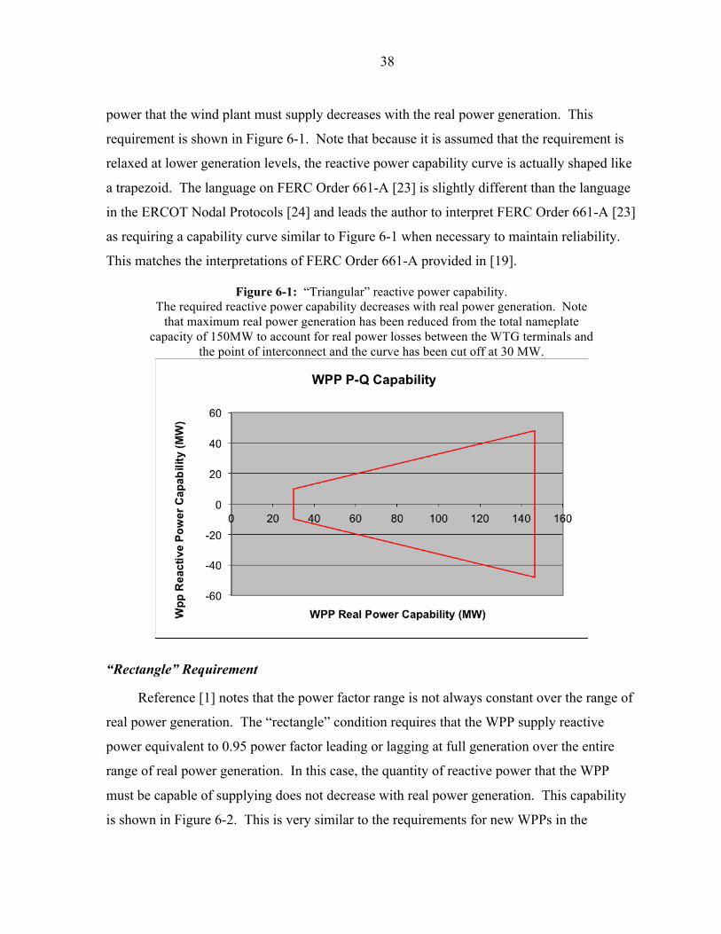
38
power that the wind plant must supply decreases with the real power generation. This
requirement is shown in Figure 6-1. Note that because it is assumed that the requirement is
relaxed at lower generation levels, the reactive power capability curve is actually shaped like
a trapezoid. The language on FERC Order 661-A [23] is slightly different than the language
in the ERCOT Nodal Protocols [24] and leads the author to interpret FERC Order 661-A [23]
as requiring a capability curve similar to Figure 6-1 when necessary to maintain reliability.
This matches the interpretations of FERC Order 661-A provided in [19].
Figure 6-1: “Triangular” reactive power capability. The required reactive power capability decreases with real power generation. Note
that maximum real power generation has been reduced from the total nameplate capacity of 150MW to account for real power losses between the WTG terminals and
the point of interconnect and the curve has been cut off at 30 MW.
“Rectangle” Requirement
Reference [1] notes that the power factor range is not always constant over the range of
real power generation. The “rectangle” condition requires that the WPP supply reactive
power equivalent to 0.95 power factor leading or lagging at full generation over the entire
range of real power generation. In this case, the quantity of reactive power that the WPP
must be capable of supplying does not decrease with real power generation. This capability
is shown in Figure 6-2. This is very similar to the requirements for new WPPs in the

39
ERCOT Nodal Protocols [24] and somewhat similar to the requirements of the UK Grid
Code [57].
Figure 6-2: Rectangular reactive power capability requirement. Note that the required reactive power capability does not decrease with real power
generation. As in Figure 6-1, the maximum real power generation has been reduced to reflect the losses between the WTG terminals and the point of interconnect.
Scenario Voltage Ranges
The reactive power capability of the wind plant varies with voltage. The reactive
power supplied by shunt devices such as capacitors, reactors, and cable shunt admittance
change with the square of voltage. Reactive losses in the cable system and transformers vary
with the square of current [1] and current is obviously dependent on voltage. Additionally,
the reactive power capability of certain WTGs is dependent on terminal voltage [5].
Reference [1] notes that the minimum reactive power requirements may need to be met at
one point of interconnect voltage, or over a range of interconnect voltages. The implication
of this is that the voltage(s) at which the WPP must be able to supply the required reactive
power is an important factor in WPP design.
For the triangle and rectangle scenarios, this study investigates the difference in losses
between the optimal and uniform dispatch under two assumptions, both of which are
consistent with discussion in [1]. The first is that the wind plant is only required to have

40
sufficient reactive power resources available to meet the minimum reactive power flow
requirements when the bus voltage at the point of interconnect is at 1.0 pu. The second is
that the wind plant is required to have sufficient reactive power resources available to meet
the minimum reactive power flow at the point of interconnect when the voltage at the point
of interconnect is between 0.95 and 1.05 pu. As discussed above, it was assumed that the
reactive power flow requirements would not apply when the WPP was operating at less than
20% generation.
Substation Resources Included in Model
Table 6-2: Summary of operation scenarios studied. Note that the rectangular and triangular cases are included twice, once with the
requirement that the reactive power capability be met over a range of voltages, and the other with the requirement that the reactive power capability be met at one
specific voltage. Reactive Power Requirement
Must Specific Set Point Be Met?
Voltage Range Over Which +/-48.1 MVAR Requirement Must Be Met
Required Substation Reactive Power Equipment
Window No N/A None
Rectangular Yes 1.0 pu 1-6 MVAR, 35kV Capacitor
Rectangular Yes 0.95–1.05 pu 2-14 MVAR, 138kV Capacitors
2-15 MVAR, 138kV Reactors
Triangular Yes 1.0 pu 1-6 MVAR, 35kV Capacitor
Triangular Yes 0.95–1.05 pu 2-14 MVAR, 138kV Capacitors
OPF solutions show that the maximum real power that can be delivered to the point of
interconnect is 146.4 MW. Thus, the WPP must be capable of supplying or absorbing 48.1
MVAR in order to operate at 0.95 power factor at 100% generation. The substation reactive
power resources required to meet the power factor requirements for each of the operation
scenarios described above were determined by power flow and OPF analysis and are listed in
Table 6-2.

41
As can be seen in Table 6-2, the quantity of substation reactive power resources can be
heavily influenced by the voltage range over which the reactive power is expected to be
delivered. For example, if the WPP is expected to provide significant quantities of reactive
power with the point of interconnect bus voltage at high levels, it may not be possible to
provide this reactive power from the WTGs as the voltage rise caused by reactive power flow
in the WTG and substation transformers may be objectionable. If this is the case, it may be
necessary to install substantial reactive power resources on the substation high voltage bus.
Additionally, if the WPP is expected to absorb significant quantities of reactive power with
the point of interconnect bus voltage at low levels, the voltage drop caused by reactive power
flow in the WTG and substation transformers may be objectionable.
Cases Studied
Several cases were run for the scenarios listed above. These cases are intended to cover
the full range of operation and are used to determine the difference in system losses between
the two reactive power dispatch strategies. These include cases in which the voltage at the
point of interconnect was at 0.95 pu, 0.975 pu, 1.0 pu, 1.025 pu, and 1.05 pu. Reference [58]
specifies that the maximum voltage for a 138kV system is 145kV or 1.05 pu. This is used as
the upper limit for the purposes of this case study. An arbitrary lower limit of 0.95 pu is
used. While specific systems may occasionally operate outside of these limits, it is assumed
that they would be of short duration and would not have a significant influence on the results
though no data was available to confirm this.
For each of the four scenarios that required the WPP to meet a specific set point, cases
were also run over a range of power factors. For the “triangle” reactive power requirement,
cases were run at 0.95 and 0.975 power factor lag, 1.0 power factor, and 0.975 and 0.95
power factor lead. The choice of 0.95 power factor leading and lagging is based on [23] and.
For the “rectangle” power factor requirement, cases were run with reactive power injections
of +/-48.1 MVAR, +/- 33.4MVAR supply, and 0 MVAR. These are based on 0.95 and 0.975
power factor lag, 1.0 power factor, and 0.975 and 0.95 power factor lead at full generation
and are similar to the windows set by [24].

42
For each of the four scenarios that required the WPP to meet a specific voltage set
point, 260 cases were run. Of these, 130 cases each were run with the turbines dispatched
optimally and another 130 cases each with the turbines dispatched uniformly. Of these 130
cases, 25 cases each were run with the WPP at 100%, 80%, 60%, 40%, and 20% generation.
These 25 cases included five cases each with the 138kV bus at 0.95 pu, 0.975 pu, 1.0 pu,
1.025 pu, and 1.05 pu. These five cases covered operation of the WPP at unity power factor,
two cases with the WPP operating with a leading power factor, and two cases with the WPP
operating with a lagging power factor. The remaining five cases were run with the WPP
operating 0% generation (no wind). These five cases covered operation with the 138kV bus
at 0.95 pu, 0.975 pu, 1.0 pu, 1.025 pu, and 1.05 pu, and it was assumed that the WPP would
operate to control the reactive power flow at the point of interconnect to 0 MVAR, though
there is no specific basis for this assumption.
For the first “window” scenario, 30 cases each were run for the optimal and uniform
dispatch. These covered operation at 100%, 80%, 60%, 40%, 20%, and 0% with the 138kV
bus voltage operating at 0.95 pu, 0.975 pu, 1.0 pu, 1.025 pu, and 1.05 pu.
Uniform Dispatch System Limitations
The only limitations placed on the uniform dispatch solutions are caused by the
capability of the WTGs. Figure 4-7 and Table 4-5 in [42] describe a portion of the dynamic
model of one manufacturer’s DFIG WTG. These imply that logic exists to prevent the
terminal voltage at the WTG from straying above 1.10 pu or below 0.90 pu on a steady state
basis though the model description does not confirm this. For the purposes of this study, it is
assumed that the controls in the individual WTGs will have logic capable of overriding the
reactive power request from the central control system if this request would cause the
terminal voltage (690V bus) to fall outside of the range between 0.90 pu and 1.10 pu and
reduce (or increase) the reactive power request to keep the WTG within its limits. It is also
assumed that the centralized control system would not act to limit voltages on the 35kV
collection system.

43
Optimal Dispatch System Limitations
One major advantage of using the OPF-based centralized control is the ability to
prevent the system from operating in a fashion that would exceed predetermined limits. The
limits placed on the OPF solution and the justifications for them are described in the
following paragraphs.
Current Limitations
In the design of new large-scale WPPs, the maximum load is determined by the total
maximum WTG generation capability. This is easy to calculate, and WPP collection systems
are generally deliberately designed such that current limitations will not be exceeded.
Voltage Limitations
The discussion of voltage limitations provided in this section is based on analysis used
by author and author’s coworkers in the design of several medium voltage collection
systems.
• Reference [10] specifies a maximum continuous operating voltage of 36.6kV or
1.061 pu on a 34.5kV base for cable elbows.
• Reference [11] specifies a maximum design voltage of 22kV for 35kV
terminators. This is 1.10 pu on 34.5kV base
• Reference [12] does not specify a maximum continuous operating voltage for
cable splices. For the purposes of this paper, it is assumed that the equipment
ratings would not be more restrictive than ratings of the cable and elbows.
• Reference [13] specifies that the operating voltage for underground cable should
not be higher than the rated voltage by more than 5% continuously and 10% for
an emergency lasting not longer than 15 minutes. This implies that 35kV cable
should not be operated continuously in excess of 36.75kV, or 1.065 pu on a
34.5kV base, and that the cable should not operate at a voltage higher than
1.116 on a 34.5kV base for longer than 15 minutes.

44
• Reference [45] limits the secondary voltage to 1.05 pu at full nameplate kVA
rating and 0.80 power factor and 1.10 pu at no load. This implies that the
primary winding voltage is allowed to be whatever is necessary to achieve a
1.05 pu secondary voltage. In the case of a WTG step up transformer, [59]
defines the primary winding as the low voltage winding and the secondary
winding as the medium-voltage winding provided that the transformer is
suitable for step-up operation. The normal service conditions defined in [45]
are for step down operation. If the 1750kVA transformer described in Chapter
5 is loaded to 1750kVA at 0.80 pf, the voltage rise through the transformer
would result in a 690V winding voltage of approximately 1.09 pu. This
calculation is shown in (6.1) below.
1.05+ 0.0074+ j0.0574( )• 0.8− j0.6( ) =1.091 (6.1)
The 690V winding voltage that would result from operating the WTG at full
rated real and reactive power (1500kW and 726kVAR) is approximately 1.08pu.
This calculation is shown in (6.2) below.
1.05+ 0.0074+ j0.0574( )•1500− j7261750
=1.081 (6.2)
• Surge arresters are commonly used in the medium-voltage collection system to
protect the cable and transformers from voltage transients. Reference [60]
recommends choosing surge arresters with 27kV duty cycle ratings for the
substation transformer and 30kV duty cycle ratings elsewhere. These
correspond to maximum continuous overvoltage ratings of 22kV and 24.4kV
(line to ground), respectively [61]. This is 1.104 and 1.225 pu on a 19.92kV
base. Reference [61] recommends utilizing an arrester with an MCOV rating
that is higher than the maximum expected phase-ground voltage.
The voltage limitations on the 34.5kV buses were set at 0.88 and 1.075 pu. The upper
limit is somewhat above the voltage levels described in the standards referenced above which
would imply a limit of 1.05 or 1.061 pu but allows for the WTG to operate closer to full

45
reactive capability. This is consistent with the limits operating voltage limits typically
utilized by author and author’s coworkers.
The minimum and maximum WTG terminal (690V) buses were set at 0.90 and 1.10 pu
as discussed above.
MATPOWER Model
A model was built in the MATPOWER software package [41]. All branches
(transformers and cable segments) and WTGs were modeled explicitly. The substation
138kV bus was treated as the slack bus. A load equal to the total WTG production as
measured at the WTG terminals (i.e., 150MW for the 100% generation cases; 120 MW the
80% generation cases) was placed at the substation 138kV bus so that the slack generator
would only supply system losses.
The MATPOWER software package does not have the capability to minimize system
losses, but does provide an AC OPF algorithm that can minimize generation cost [41]. For
the optimal model, both the upper and lower voltage limits on the substation 138kV bus were
placed at the value desired for that particular case. The reactive load on the substation
138kV bus was set at the level that was required to be delivered to the bulk transmission
system for that particular case. The incremental cost for the WTGs was set at $0/MWHr.
The slack bus generator was set at $80/MWHr to force the slack generator to generate as
little real power as possible. These values were arbitrarily chosen, any values would suffice
as long as the incremental costs for the WTGs were lower than the slack bus generator. For
the slack bus generator, the maximum and minimum reactive power generation were set to
zero to force all reactive power to be generated by the WPP. The maximum power limit for
each WTG was set at the desired value for that case (i.e., 1.5 MW for 100% generation, 1.2
MW for 80% generation, etc).
MATPOWER also possesses a standard AC power flow algorithm that was used for the
uniform cases. For these cases, the WTG real power generation was set at the required level.
The slack bus voltage was set at the value desired for that case. The slack bus load was set
with zero reactive power demand. Each WTG was treated as a P-Q bus with the real power
injection set to the desired value for that case (i.e., 1.5 MW for 100% generation, 1.2 MW for

46
80% generation, etc). The reactive power injection for each WTG was changed until the
reactive power injection by the slack bus generator reached the desired value. If a particular
WTG 690V bus voltage reached dropped below 0.90 pu or exceeded 1.10 pu, that unit was
changed to a P-V bus and the other WTG reactive power injections were adjusted
accordingly.
Results
In total, 1100 cases were run. The differences in losses between the optimal and
uniform dispatch were then compared for each case. A summary of the potential energy
savings at 100% generation created by optimally dispatching reactive power resources is
provided in Table 6-3.
Table 6-3: Summary of potential real power savings at 100% generation. Note that in certain cases, the optimal reactive power dispatch actually produces
higher losses than the uniform dispatch case due to the additional voltage constraints imposed on the solution.
Reactive Power Requirement Voltage Range Over Which +/-48.1 MVAR Requirement Must Be Met
Range of Potential Power Savings Due to Optimal Dispatch of Reactive Power (kW)
Window N/A 6.8–11.3
Rectangular 1.0 pu -304.6–127.0
Rectangular 0.95–1.05 pu -230.0–354.0
Triangular 1.0 pu -304.2–127.0
Triangular 0.95–1.05 pu -230.3–197.2
The cases in which the optimal solution actually produced higher losses are caused by
the voltage constraints that are placed on the optimal reactive power strategy but not on the
uniform strategy. These cases are expected to occur infrequently as they are caused by cases
where the transmission system voltage is low and the WPP is absorbing large quantities of
reactive power or the transmission system voltage is high and the WPP is generation large
quantities of reactive power.
The difference in losses was then multiplied by the hours per year that the WPP would
be expected to operate at that particular level. From this information, the total difference in

47
losses between the various scenarios can be calculated. Unfortunately, data showing how
many years a typical WPP operates at a given level were not available and were estimated.
In estimating the number of hours per year that the WPP would operate at a particular level,
the assumptions listed below were made.
• When a specific set point is required to be met, the WPP will control voltage at the
point of interconnect to a value that varies based on system conditions but will be
between 1.0 pu and 1.05 pu.
• The WPP will be connected to a system that is neither strong nor weak, implying that
the WPP will have a significant impact on system voltage levels, but will not always
be capable of supplying (or absorbing) sufficient reactive power to regulate the bus
voltage to the desired set-point. This implies that the bus voltage will stray from the
set point during normal operation, but should remain close.
• The WPP will spend the hours listed in Table 6-4 per year at each respective
generation level, regardless of the case. This data was taken from the average of
several recent WPP projects.
Table 6-4: Hours spent per year at each generation level. Note that this produces a yearly capacity factor of approximately 46%.
Generation Level
Hours/Year
100% 1100
80% 1300
60% 1400
40% 1600
20% 2000
0% 1360
With the assumptions described above, the hours that WPP operations would
approximate each case was estimated, and the total difference in losses between the uniform
and optimal dispatch were calculated and appear in Table 6-5.

48
Table 6-5: Estimated annual energy savings. Reactive Power Requirement
Voltage Range Over Which +/-48.1 MVAR Requirement Must Be Met
Estimated Annual Energy Savings (MWhr)
Window N/A 18
Rectangular 1.0 pu 372
Rectangular 0.95–1.05 pu 1,358
Triangular 1.0 pu 140
Triangular 0.95–1.05 pu 339

49
Chapter 7 Discussion of Results
System Losses
The results show that the majority of the difference between the optimal and uniform
dispatches comes from utilizing the substation reactive power resources more effectively. To
demonstrate this, five cases were run using the “rectangular” case with the 0.95 –1.05 pu
voltage requirement. The uniform reactive power dispatch strategy described in Chapter 6
was used except that the substation resources were utilized in the same manner as the results
from the optimal dispatch strategy. The results of this are shown in Table 7-1.
Table 7-1: Comparison between substation resource dispatch strategies. “Uniform-Optimal” utilizes the original uniform dispatch strategy. “Uniform
Alternate-Optimal” utilizes the alternate dispatch described above. Difference in Losses (kW)
Reactive Power Flow at POI
48.1 MVAR Supply
33.4 MVAR Supply
0 MVAR
33.4 MVAR Absorb
48.1 MVAR Absorb
Uniform - Optimal 147.5 178.6 6.3 204.1 347.3
Uniform Alternate - Optimal 27.9 10.5 6.3 4.1 1.4
The OPF results for the “window” cases offer some insight as to the optimal operating
point for the WPP. Surprisingly, the results show that it is most efficient for the wind farm to
deliver between 1.4 and 4.1 MVAR to the point of interconnect depending on the voltage at
the point of interconnect. It was anticipated that the optimal operating point would be to
have the WPP absorb modest quantities of reactive power.
Reactive Power Injections
Normal Conditions
As expected, the results show an inverse relationship between the total resistance
measured at the WTG terminals and the reactive power injection under normal operating

50
conditions. Also as expected, the WTGs that are closest electrically to the point of
interconnect inject the most reactive power while the WTGs that are furthest electrically
inject the least. This relationship is illustrated in Figure 7-1, which shows a plot of the
reactive power injected by the WTGs on two of the test system’s six collection circuits
versus total resistance between the WTG terminals and the point of interconnect. Circuit
F1B is the collection circuit containing the WTG that is electrically closest to the point of
interconnect. Circuit F4 contains the most electrically distant WTG. The case shown in
Figure 7-1 was chosen because it was assumed that this would be the maximum generation
case that occurs most frequently.
Figure 7-1: WTG reactive power injection versus system resistance under normal conditions utilizing the optimal reactive power dispatch strategy.
Note that only two collector circuits are shown for clarity. The figure shows the results for Case 18 from the “triangular” reactive power requirement.
As can be seen in Figure 7-1, the relationship between resistance to the point of
interconnect and reactive power injection is not perfect. This is to be expected because losses
in a given branch are proportional to resistance multiplied by the square of the current and
the optimal reactive power injection is therefore dependent on the other WTGs. The case
shown in Figure 7-1 is expected to be a fairly common occurrence. In this case, the WPP is
operating at full capacity, is supplying 0 MVAR to the transmission system, and the point of

51
interconnect is operating at 1.025 pu. In this case, the solution is not limited by any voltage
constraints.
Extreme Conditions
Figure 7-2: WTG reactive power injection versus system impedance under extreme conditions utilizing the optimal dispatch strategy.
Note that the x-axis begins at 3.4 pu. Total system impedance is used in lieu of the system resistance that was used in Figure 6-1 as voltage rise is affected by total
system impedance. This figure shows the results for Case 21 from the “triangular” reactive power requirement.
While the results show that the optimal reactive power controller will generally reduce
system losses, under certain situations, the optimal solution will actually produce losses that
exceed those produced by the uniform cases. This is due to more restrictive voltage
constraints that are imposed on the optimal solution over the similar cases utilizing the
uniform dispatch method. These situations arise in two fashions. The first is where the
interconnect bus voltage is high and the WPP is expected to supply significant quantities of
reactive power. In these cases, 34.5kV bus voltages restrain the OPF and some of the
electrically more distant WTGs absorb reactive power to reduce the voltages on the more
remote 34.5kV buses. The WTGs that are closer to the substation in turn generate additional
reactive power to compensate. A similar situation occurs at low interconnect bus voltages
(0.95 pu) when the WPP is being asked to absorb reactive power. The cases where this

52
happens are expected to occur infrequently but are more extreme in cases where the WPP
does not have significant substation reactive power resources.
Figure 7-3: WTG reactive power injection versus system impedance under extreme conditions utilizing the uniform dispatch strategy.
Note that only two collector circuits are shown for clarity and that the x-axis begins at 3.4 pu. This figure shows the results for Case 21 from the “triangular” reactive
power requirement.
Figure 7-2 and Figure 7-3 are scatter plots of reactive power injections versus system
impedances for Case 21 with the “triangular” reactive power requirement. In this case, the
bus voltage at the point of interconnect is 1.05 pu and the WPP is asked to deliver maximum
reactive power. Figure 7-2 shows a plot of the reactive power injected by the WTGs on two
of the test system’s six collection circuits versus total system impedance between the WTG
terminals and the point of interconnect.
Figure 7-2 clearly shows that when utilizing the optimal dispatch algorithm, the WTGs
can be divided into two groups. The first group is injecting close to maximum reactive
power; the second, smaller, group is absorbing close to maximum reactive power to hold bus
voltages on the medium-voltage collection system within limits. In this case, the correlation
between reactive power injection and system impedance is significantly less than in the case
depicted in Figure 7-1. However, the general trend is that the WTGs that are more distant
electrically from the point of interconnect are more likely to be absorbing reactive power

53
than the WTGs that are closer to the point of interconnect. There is a significant contrast
between the reactive power injections shown in Figure 7-2 and the injections from the
corresponding uniform dispatch case, which are shown in Figure 7-3.
As can be seen in Figure 7-3, the reactive power injections are uniform with the
exception of some of the more distant WTGs, whose injections are reduced to prevent the
WTG terminal voltage from exceeding 1.10 pu. Note that in the uniform dispatch case, all
WTGs inject reactive power into the system and none absorbs reactive power. This is
significantly different from the results obtained utilizing the optimal dispatch algorithm.
Voltage Profile
Normal Conditions
Also of interest are the differences between the voltage profiles created by the two
reactive power dispatch methods. A plot of 34.5kV bus voltages versus system impedance
created by the optimal dispatch method is shown in Figure 7-4. Note that these bus voltages
are from the same case as the reactive power injections in Figure 7-1.
Figure 7-4: WTG 34.5kV bus voltage versus system impedance under normal conditions utilizing the optimal dispatch strategy.
This figure shows the results for the optimal strategy for Case 18 from the “triangular” reactive power requirement.

54
Figure 7-5 shows a plot of bus voltages versus system impedance for the same case as
Figure 7-4 but with the results from the uniform dispatch method. As can be seen by
comparing Figure 7-4 to Figure 7-5, the voltage profile created by the two dispatch strategies
is similar under normal circumstances. Table 7-2 shows a summary of the 35kV bus voltage
profiles resulting from Case 18 with the “triangular” reactive power requirement.
Figure 7-5: WTG 34.5kV bus voltage versus system impedance under normal conditions utilizing the uniform dispatch strategy.
This figure shows the results for the uniform strategy for Case 18 from the “triangular” reactive power requirement.
Table 7-2: Summary of voltage profiles created by two reactive power dispatch strategies under normal conditions.
Optimal Strategy
Uniform Strategy
Minimum 34.5kV Bus Voltage
1.0165 pu 1.0165 pu
Maximum 34.5kV Bus Voltage
1.0477 pu 1.0504 pu
Average 34.5kV Bus Voltage
1.0283 pu 1.0293 pu
Table 7-2 shows that under conditions where bus voltages are less than the constraints,
the voltage profiles created by the two dispatch strategies are similar. The voltage profile for

55
the optimal strategy is somewhat less than the uniform strategy; however, some of this is due
to the fact that the optimal solution deployed one 6 MVAR substation capacitor whereas the
uniform strategy deployed none.
Extreme Conditions
Under extreme conditions, the voltage profile created by the two strategies differs
significantly. The optimal strategy is forced to constrain the 34.5kV bus voltages to 1.075pu,
whereas the uniform strategy only restricts the 690V bus voltages to 1.10 pu or less. Figure
7-6 and Figure 7-7 show the voltage profile on the 34.5kV system under the same conditions
as the scatter plots in Figure 7-2 and Figure 7-3. The voltage profile created by the optimal
strategy under these conditions is shown in Figure 7-6.
Figure 7-6: WTG 34.5kV bus voltage versus system impedance under extreme conditions utilizing the optimal dispatch strategy.
This figure shows the results for the optimal solution to Case 21 with the “triangular” reactive power requirement.
The voltage profile created by the uniform dispatch strategy under the same conditons
as the results shown in Figure 7-6 is shown in Figure 7-7. These figures clearly show that
there is a siginificant difference between the voltage profiles created using the optimal and

56
uniform strategies under more extreme conditions. As can be seen in Figure 7-6, the
requirement to maintain the 34.5kV bus voltages at or below 1.075 is a much more severe
requirement than the requirement to maintain the 690V bus voltages at no more than 1.10 pu.
Table 7-3 shows a summary of the collection system 34.5kV bus voltages under the more
extreme conditions. Note that the bus voltages created by the uniform strategy are
significantly higher than the voltages created by the optimal strategy.
Figure 7-7: WTG 34.5kV bus voltage versus system impedance under extreme conditions utilizing the uniform dispatch strategy.
This figure shows the results or the uniform solution to Case 21 with the “triangular” reactive power requirement.
Table 7-3: Summary of bus voltage profiles created by two reactive power strategies under extreme conditions.
Optimal Strategy
Uniform Strategy
Minimum 34.5kV Bus Voltage
1.0576 pu 1.0571 pu
Maximum 34.5kV Bus Voltage
1.0750 pu 1.0908 pu
Average 34.5kV Bus Voltage
1.0679 pu 1.0706 pu

57
Cost Effectiveness
The net present value method of making project investment decisions is described in
[62]. In order to determine the present value of the losses that are avoided by using the
proposed control strategy over the “uniform” strategy, it is first necessary to determine the
present value of the avoided losses and the present value of incremental expenditures
necessary to purchase and install the OPF based control system. The net present value is
then the money remaining after the present value of the incremental cost of the improvements
is subtracted from the present value of the avoided losses.
Present Value of Avoided Losses
The present value of the avoided losses is obviously dependent on the cost of the
energy produced by the WPP. Lawrence Berkeley National Laboratory has compiled market
data on WPPs and the power purchase agreements (PPA) through which the energy is
typically sold. A summary of this research is provided in [63]. The typical WPP built in
2009 averaged 91 MW, was owned by an independent power producer, and the energy was
sold through a long term PPA. For projects constructed in 2009, the average sale price of
wind energy sold under a power purchase agreement was $61/MWhr [63]. According to
Figure 20 in [63], PPA prices for projects completed in 2009 ranged from $40/MWhr to
$85/MWhr. These prices do not include the renewable energy production tax credit (PTC)
[63]. Discussion in [64]–[66] provides an outline of a PPA that was proposed in proceedings
before the Iowa Utilities Board. In this case, an independent power producer offered to sell
energy from two WPPs for a period of 25 years at a cost of $54.06/MWhr with a yearly cost
increase of 2% [64], [65].
The PTC is available for the first 10 years after commercial operation commences and
is adjusted for inflation [67], [68]. In tax year 2010, the value of this tax credit was
$0.022/kWhr or $22/MWhr [68], [69].
Discussion in [66] quotes testimony from the independent power producer where they
stated that they generally do not proceed with a project unless the return on equity is in “the
teens or the twenties” (quoted on p. 80) whereas the regulated utility was requesting a return
on equity of 12.2% to build its own WPPs [66].

58
Reference [70] provides formulas for calculating the present value of a series of cash
flows. The formula for calculating the present value of a geometrically increasing series is
provided in Equation (4.26) in [70] (p. 147). This is repeated in (7.1) below.
P = A11− 1+ g( )N 1+ i( )−N
i− gif i ≠ g
or
P = N ⋅A11+ i
if i = g
(7.1)
Where:
• P is the present value of the series of cash flows
• A1 is the cash flow at the end of the first period
• g is the change, in percent, of the cash flow between consecutive periods
• i is the interest rate
• N is the number of periods
Table 7-4: Summary of loss value scenarios. High Energy
Value Middle Energy Value
Low Energy Value
Initial PPA Energy Price ($/MWhr)
$80 $60 $40
Minimally Attractive Rate of Return (%)
10% 15% 20%
PPA Escalation (%/year) 2% 2% 2%
PPA Duration (years) 25 25 25
Initial PTC Value ($/MWhr) $22 $22 $22
PTC Inflation Adjustment (%/year)
3.2% 3.2% 3.2%
PTC Duration (Years) 10 10 10
Calculated Present Value of Avoided Losses ($/MWhr)
$1000 $560 $320

59
It is possible to calculate a range of possible values for a MWhr of loss that is avoided
each year. Because of the substantial variation in values provided in the information above,
three scenarios were calculated using (7.1) and are shown in Table 7-4. The assumed
inflation rate is based on information presented in [71] which implies an annual inflation rate
of 3.2% in the 30 years between 1981 and 2010.
Present Value of Costs of the Proposed Control System
It is difficult to forecast the costs of the proposed control system and the Author is not
aware of any published data that would serve as a useful reference. As mentioned in Chapter
4, much of the hardware necessary to implement the control system is already present at most
WPPs. The development costs for the control software would be spread across several
WPPs; however, there would be costs associated with setting up and tuning the algorithm for
each individual WPP. Estimated incremental costs associated with the installation and
maintenance of the proposed system were calculated using (7.1) and are given in Table 7-5.
Table 7-5: Assumed incremental costs of proposed control system. High Energy
Value Middle Energy Value
Low Energy Value
Upfront Set-Up Costs $100 000 $100 000 $100 000
Average Yearly Maintenance Costs ($/Year)
$10 000 $10 000 $10 000
Minimally Attractive Rate of Return (%)
10% 15% 20%
Inflation Rate (%/year) 3.2% 3.2% 3.2%
Site Life (years) 25 25 25
Calculated Present Value of System Costs
$220 000 $180 000 $160 000
The estimates presented in Table 7-5 are not based on any published data but rather on
the assumption that the proposed system is an incremental improvement over the centralized
control systems that are already installed at a large number of WPPs.

60
Net Present Value of Proposed Control System
Using the values presented in Table 6-5, Table 7-4, and Table 7-5, it is possible to
calculate the net present value of the proposed control system. The estimated net present
value of the control system proposed in Chapter 4 is shown in Table 7-6. As expected, the
cost effectiveness depends heavily on the amount of reactive power that the WPP is expected
to provide to the transmission system and the value of the energy. Using the assumptions
described above, the proposed control system can be justified on the basis of cost savings in
7 of the 15 cases that were analyzed.
Table 7-6: Estimated net present value of proposed control system. Reactive Power Requirement
Voltage Range Over Which +/-48.1 MVAR Requirement Must Be Met
Estimated Annual Energy Savings (MWhr)
High Value Energy
Middle Value Energy
Low Value Energy
Window N/A 18 ($202 000) ($169 920) ($154 240)
Rectangular 1.0 pu 372 $152 000 $28 320 ($40 960)
Rectangular 0.95–1.05 pu 1,358 $1 138 000 $580 480 $274 560
Triangular 1.0 pu 140 ($80 000) ($101 600) ($115 200)
Triangular 0.95–1.05 pu 339 $119 000 $9 840 ($51 520)
Significant Assumptions
Several significant assumptions that were made and conjecture on their potential impact
on the study results are given below.
• While there has been some discussion of centralized control systems in the literature,
a discussion of which is provided in Chapter 4, the strategies used by commercial
centralized control systems is unknown. The author has utilized the uniform dispatch
method described here for recent studies; however, it should not be considered an
accurate representation of a commercially available system.
• As discussed above, a significant portion of the difference between the optimal and
uniform dispatch methodologies comes from the assumption that the uniform dispatch
will utilize the substation resources last, whereas the optimal dispatch tends to use

61
them first. If it were assumed that the uniform dispatch utilized the substation
reactive power resources first, the difference between the two methods would be less.
• Data showing the hours that the WPP would spend at each generation level were
taken from the average of several sites and are believed to be typical.
• Data showing the variation of the interconnect bus voltage and reactive power
injections over time were not available and would likely vary considerably from
location to location. This means that the hours spent operating at each case were not
available, and assumptions were made to create this data.
• This study assumes that the WTGs will all operate at the highest real power injection
allowed by the prevailing winds at all times. For simplicity, it was assumed that all
WTGs would operate at an equal generation level. Under normal operations, the
wind speed may be different across the wind plant. This may cause individual WTGs
to produce different levels of real power at the same time [30].
• No data was available to provide an accurate cost estimate of the incremental costs of
the proposed control system. Data used to determine cost effectiveness is estimated.
Conclusion
Using the data presented here, it appears that while a centralized control system that
integrates an OPF algorithm will reduce system losses, the reduction in losses is smaller than
the author had anticipated. An important advantage of this control system is the ability to
force the reactive power dispatch to respect voltage constraints.
It appears that an economic justification for utilizing the proposed OPF based
centralized control system may exist at WPPs with higher energy values. The author feels
that the control system would be most useful in very large WPPs with long collection
circuits. In these WPPS, the long collection circuits cause increased losses and voltage
regulation problems and a control system that accounts for the system impedance between
the WTG terminals and the point of interconnect would provide the most benefits in such a
system.

62
Oportunities for Further Work
Opportunities for further advancement of the control system are provided in Chapter 4.
The analysis of cost effectiveness could be refined in several ways. Most of these revolve
around clarifying the significant assumptions listed above. The estimate of the incremental
loss savings could be improved by using real WPP systems with historical data showing the
number of hours that the wind plant operates at various combinations of interconnect bus
voltage and real and reactive power injections. Additionally, the estimate of incremental loss
savings could be improved by comparing the proposed control system to a commercial
control system. The economic analysis could be improved by using economic data from
actual projects and by developing a detailed estimate of the incremental cost to install the
proposed OPF based centralized control system.
This thesis has presented detailed steady-state studies. Another possibility for further
study is detailed time-domain studies to show the dynamic performance of the control system
to changing system conditions.

63
References
[1] Wind Power Plant Collector Design WG, “Reactive power compensation for wind power plants,” presented at the 2009 Power and Energy Soc. General Meeting, Calgary, Canada.
[2] Wind Power Plant Collector Design WG, “Wind power plant collector system design considerations,” presented at the Proc. 2009 Power and Energy Soc. General Meeting, Calgary, Canada.
[3] Wind Power Plant Collector Design WG, “Wind plant collector system fault protection and coordination,” presented at the Transmission and Distribution Conf. and Exposition, New Orleans, LA, 2010.
[4] Wind Power Plant Collector Design WG, “Design and application of cables and overhead lines in wind power plants,” presented at the Transmission and Distribution Conf. and Exposition, New Orleans, LA, 2010.
[5] Wind Power Plant Collector Design WG, “Characteristics of wind turbine generators for wind power plants,” presented at the 2009 Power and Energy Soc. General Meeting, Calgary, Canada.
[6] Wind Power Plant Collector Design WG, “Wind power plant substation and collector system redundancy, reliability, and economics,” presented at the 2009 Power and Energy Soc. General Meeting, Calgary, Canada.
[7] Wind Power Plant Collector Design WG, “Wind power plant grounding, overvoltage protection, and insulation coordination,” presented at the 2009 Power and Energy Soc. General Meeting, Calgary, Canada.
[8] Wind Power Plant Collector Design WG, “Arc-flash hazard in wind power plants,” in Transmission and Distribution Conf. and Exposition, New Orleans, LA, 2010.
[9] Wind Power Plant Collector Design WG, “Power transformer application for wind plant substations,” presented at the Transmission and Distribution Conf. and Exposition, New Orleans, LA, 2010.
[10] IEEE Standard for Separable Insulated Connector Systems for Power Distribution Systems Above 600 V, IEEE Standard 386-2006.
[11] IEEE Standard Test Procedures and Requirements for Alternating Current Cable Terminations 2.5kV Through 765kV, IEEE Standard 48-1996.
[12] IEEE Standard for Extruded and Laminated Dielectric Shielded Cable Joints Rated 2500V to 500,000V, IEEE Standard 404-2006.
[13] Standard for Concentric Neutral Cables Rated 5 through 46kV, ANSI/ICEA Standard S-94-649-2004.
[14] A. R. Bergen, V. Vittal, 2000. “Power flow analysis” in Power Systems Analysis, 2nd ed., Upper Saddle River, Prentice Hall, 2000, chap. 10, sec. 10.1–8, pp. 325–356.

64
[15] J. D. McCalley, “Power flow 2,” Unpublished lecture notes for EE 456, Fall Semester, 2006, Iowa State University.
[16] J. D. McCalley, “Obtaining the jacobian,” Unpublished lecture notes for EE 456, Fall Semester, 2006, Iowa State University.
[17] J. D. McCalley, “Fast power flow methods,” Unpublished lecture notes for EE 456, Fall Semester, 2006, Iowa State University.
[18] American Wind Energy Association. (2011, April). 2010 U.S. Wind Industry Market Update. [Online]. Accessed 8/13/11. Available: http://www.awea.org/learnabout/publications/factsheets/upload/Market-Update-Factsheet-Final_April-2011.pdf.
[19] R. J. Konopinski, P. Vijayan, V. Ajjarapu, “Extended reactive capability of DFIG wind parks for enhanced system performance,” IEEE Trans. Power Syst., vol. 24, no. 3, pp. 1346–1355, August 2009.
[20] X. R. Zhu, Y. Wang, C. Fu, “Strategy of reactive power and voltage control in large wind farms integrated region,” in 2010 Int. Conf. on Power Syst. Tech., Hangzhou, China.
[21] S. Engelhardt, I. Erlich, C. Feltes, J. Kretschmann, F. Schewarega, “Reactive power capability of wind turbines based on doubly fed induction generators,” IEEE Trans. Energy Convers., vol. 26, no. 1, pp. 364–372, March 2011.
[22] Y. Lei, A. Mullane, G. Lightbody, R. Yacamini, “Modeling of the Wind Turbine with a Doubly Fed Induction Generator for Grid Integration Studies.” IEEE Trans. Energy Convers., vol. 21. no. 1, pp. 257–264, March 2006.
[23] Federal Energy Regulatory Commission. (2005, December) Order 661-A. Interconnection for Wind Energy (Order on Re-Hearing and Clarification), Docket No. RM05-4-001.
[24] Electric Reliability Council of Texas. (2011, Sep. 1) ERCOT Nodal Protocols Section 3 Management Activities for the ERCOT System, 2011, pp. 3-115–121.
[25] M. Wilch, V. S. Pappala, S. N. Singh, I. Erlich, “Reactive power generation by DFIG based wind farms with AC grid connection,” in IEEE Powertech, Lausanne, 2007, pp. 626–632.
[26] V. S. Pappala, M. Wilch, S. N. Singh, I. Erlich, “Reactive power management in offshore wind farms by adaptive PSO,” presented at the 2007 Int. Conf. Intelligent Syst. Applications to Power Syst., Kaohsiung, Taiwan, 2007.
[27] N. Miller, P. Marken, “Facts on grid friendly wind plants,” presented at the Proc. Power and Energy Soc. General Meeting, Minneapolis, MN.
[28] A. Tapia, G. Tapia, J. X. Ostolaza, J. R. Saenz, R. Criado, J. L. Berasategui, “Reactive power control of a wind farm made up with doubly fed induction generators (II),” in Proc. IEEE Powertech, Porto, 2001, vol. 4.

65
[29] D. Xu, R. Li, Y. Liu, L. Lang, “Reactive power analysis and control of doubly fed induction generator wind farm,” presented at the 13th European Conf. on Power Electron. and Applicat., Barcelona, Spain, 2009.
[30] A. Beugniez, T. Ghennam, B. Francois, E. M. Berkouk, B. Robyns, “Centralized supervision of reactive power generation for a wind farm,” presented at the 12th European Conf. on Power Electron. and Applicat., Aalborg, Denmark, 2007.
[31] G. Tapia, A. Tapia, J. X. Ostolaza, “Proportional-integral regulator-based approach to wind farm reactive power management for secondary voltage control,” IEEE Trans. Energy Convers., vol. 22, no. 2, pp. 488–498, June 2007.
[32] N. Chen, Y. Fu, L. Huang, “Prioritizing reactive power assignment strategy for doubly fed induction generation of large-scale wind farm,” in Proc. Int. Power Electron. Conf., Sapporo, Japan, 2010, pp. 262–267.
[33] W. Chengfu, Z. Li, L. Jun, Nuiyuanfang, “A new method of reactive power-voltage coordinated control in wind farm,” presented at the 2010 Asia Pacific Power and Energy Eng. Conf., Chengdu, China.
[34] W. Qiao, R. G. Harley, G. K. Venayagamoorthy, “Coordinated reactive power control of a large wind farm and a STATCOM using heuristic dynamic programming,” IEEE Trans. on Energy Convers., vol. 24, no. 2, pp. 493–503, June 2009.
[35] J. Fang, G. Li, X. Liang, M. Zhou, “An optimal strategy for reactive power in wind farms consisting of VSCF DFIG wind turbine generator systems,” in 4th International Conf. on Elect. Utility Deregulation and Restructuring and Power Technologies, Weihai, China, 2011, pp. 1709–1715.
[36] A. J. Wood, B. F. Wollenberg, “Optimal power flow” in Power Generation Operation and Control, 2nd ed. New York, Wiley, 1996, ch. 13, sec. 13.1–2, pp. 514–531.
[37] P. Kundur, “Excitation Systems” in Power System Stability and Control, New York, McGraw-Hill, 1994, ch. 8, sec. 8.5.4, pp. 335–337.
[38] IEEE Guide for the Application of Shunt Capacitors, IEEE Standard 1036-2010. [39] Z. Gajic, “Linear control systems” in Linear Dynamic Systems and Signals, Upper
Saddle River, Prentice Hall, 2002, ch. 12 sec. 12.6 pp. 599–601. [40] A. J. Wood, B. F. Wollenberg, “Optimal power flow” in Power Generation Operation
and Control, 2nd ed. New York, Wiley, 1996, ch. 13, sec. 13.3, pp. 531–534. [41] R.D. Zimmerman, C. E. Murillo-Sánchez, R. J. Thomas, "MATPOWER steady-state
operations, planning, and analysis tools for power systems research and education," in IEEE Trans. on Power Syst., vol. 26, no. 1, pp. 12–19, Feb. 2011.
[42] K. Clark, N. Miller, J. Sanchez-Gasca. (2010, April 16) Modeling of GE wind turbine-generators for grid studies Version 4.5. [Online]. Accessed 3/26/11. Available: http://www.gepower.com/prod_serv/products/utility_software/en/downloads/GE_WTG_Modeling-v4.5.pdf.
66
[43] P. Kundur, “General characteristics of modern power systems,” in Power System Stability and Control, New York, McGraw-Hill, 1994, ch. 1, sec. 1.1, pp. 3–5.
[44] IEEE Standard for Requirements for Pad-Mounted, Compartmental-Type, Self-Cooled, Three-Phase Distribution Transformers, 5 MVA and Smaller; High Voltage, 34.5 kV Nominal System Voltage and Below; Low Voltage, 15kV Nominal System Voltage and Below, IEEE Standard C57.12.34-2009.
[45] IEEE Standard for General Requirements for Liquid-Immersed Distribution, Power, and Regulating Transformers, IEEE Standard C57.12.00-2010.
[46] W. H. Kersting, “Series impedance of overhead and underground lines,” in Distribution System Modeling and Analysis, 1st ed. Boca Raton, CRC, 2002, ch. 4, sec. 4.1–2, pp. 77–105.
[47] W. H. Kersting, “Shunt admittance of overhead and underground lines,” in Distribution System Modeling and Analysis, 1st ed. Boca Raton, CRC, 2002, ch. 5, sec. 5.3–4, pp. 115–120.
[48] Southwire Company Power Cable Manual, 2nd ed. Southwire Co., Carrollton, GA, 1997, pp. 6-6, 6-14–24.
[49] Southwire Company Overhead Conductor Manual, 2nd ed., Southwire Co., Carrollton, GA, 2007, p. 1.33–34.
[50] IEEE Guide for Soil Thermal Resistivity Measurements, IEEE Standard 442-1981. [51] National Electrical Code, NFPA 70, 2011. [52] National Electrical Safety Code, IEEE Standard C2-2007. [53] IEEE Guide for the Design and Installation of Cable Systems in Power Generating
Stations, ANSI/IEEE Standard 422-1986. [54] IEEE Guide for the Application of Sheath-Bonding Methods for Single-Conductor
Cables and the Calculation of Induced Voltages and Currents in Cable Sheaths, ANSI/IEEE Standard 575-1988.
[55] Short Circuit Characteristics of Insulated Cable, ICEA Standard P-32-382-2007. [56] Short Circuit Performance of Metallic Shields and Sheaths of Insulated Cable, ICEA
Standard P-45-482-1999. [57] National Grid Electricity Transmission plc. (2011, Aug. 12) The Grid Code, Issue 4,
Revision 7, pp. CC-16–18. [58] American National Standard for Electric Power Systems and Equipment–Voltage
Ratings (60 Hertz), ANSI Standard C84.1-2006. [59] IEEE Standard Terminology for Power and Distribution Transformers, IEEE Standard
C57.12.80-2010. [60] R. A. Walling, “Overvoltage protection and arrester selection for large wind plants,”
presented at the Transmission and Distribution Conf. and Exposition, Chicago, IL, 2008.

67
[61] IEEE Guide for the Application of Metal Oxide Surge Arresters for Alternating Current Systems, IEEE Standard C62.22-2009.
[62] C. S. Park, “Present worth analysis,” in Contemporary Engineering Economics, 3rd ed. Upper Saddle River, 2002, ch. 7, sec. 7.3–4, pp. 287–304.
[63] R. Wiser, M. Bolinger, G. Barbose, N. Darghouth, B. Hoen, A. Mills, K. Porter, S. Fink, S. Tegen, “2009 wind technologies market report,” United States Department of Energy, 2010. [Online]. Accessed 10/24/11. Available: eetd.lbl.gov/ea/emp/reports/lbnl-3716e.pdf.
[64] M. O’Sullivan, direct testimony to the Iowa Utilities Board on behalf of NextEra Energy Resources, LLC, in re: “Application of MidAmerican Energy Company for the determination of ratemaking principals,” IUB Docket No. RPU-2009-0003, filed 2009, May 22. [Online]. Accessed 10/24/11. Available: https://efs.iowa.gov/efiling/groups/external/documents/docket/013955.pdf.
[65] M. O’Sullivan, Exhibit (MO-4) in direct testimony to the Iowa Utilities Board on behalf of NextEra Energy Resources, LLC, in re: “Application of MidAmerican Energy Company for the determination of ratemaking principals,” IUB Docket No. RPU-2009-0003, filed 2009, May 22. [Online]. Accessed 10/24/11. Available: https://efs.iowa.gov/efiling/groups/external/documents/docket/013957.pdf.
[66] State of Iowa, Department of Commerce, Utilities Board, Final decision and order in re: MidAmerican Energy Company, IUB Docket No. RPU-2009-0003, issued 2009, Dec. 14. [Online]. Accessed 10/23/11. Available: https://efs.iowa.gov/efiling/groups/external/documents/docket/028712.pdf.
[67] United States Code, “Electricity produced from certain renewable resources, etc.” 26 U.S.C. § 45 (2011). [Online]. Accessed 10/25/11. Available: http://uscode.house.gov/download/pls/26C1.txt.
[68] Department of the Treasury, Internal Revenue Service, “Instructions for form 8835,” 2010, cat. no., 55349M. [Online]. Accessed 10/24/11. Available: www.irs.gov/pub/irs-pdf/i8835.pdf.
[69] Department of the Treasury, Internal Revenue Service, “Renewable electricity, refined coal, and Indian coal production credit,” Form 8835, 2010, cat. no. 14954R. [Online]. Accessed 10/24/11. Available: www.irs.gov/pub/irs-pdf/f8835.pdf.
[70] C. S. Park, “Time is money,” in Contemporary Engineering Economics, 3rd ed. Upper Saddle River, 2002, ch. 4, sec. 4.3, pp. 115–150.
[71] United States Department of Labor, Bureau of Labor Statistics, “Consumer price index, all urban consumers – (CPI-U),” October 19, 2011. [Online]. Accessed 10/25/11. Available: ftp://ftp.bls.gov/pub/special.requests/cpi/cpiai.txt

68
Appendix 1 Test System Medium Voltage Cable Impedances
Table A1-1: 35kV cable impedances used in test system. From Bus Name
To Bus Name
Length (ft) Cable Type
R1 (Ohms)
X1 (Ohms)
B1 (Micro Siemens)
R1 (pu)
X1 (pu) B1 (pu)
Sub T1 5000 Al-4/0 AWG 0.5170 0.2600 80.1100 0.0434 0.0218 0.000954 T1 T2 1400 Al-4/0 AWG 0.1448 0.0728 22.4308 0.0122 0.0061 0.000267 T2 T3 1400 Al-4/0 AWG 0.1448 0.0728 22.4308 0.0122 0.0061 0.000267 T3 T4 1400 Al-4/0 AWG 0.1448 0.0728 22.4308 0.0122 0.0061 0.000267 T4 T5 1400 Al-4/0 AWG 0.1448 0.0728 22.4308 0.0122 0.0061 0.000267 T5 T6 1400 Al-4/0 AWG 0.1448 0.0728 22.4308 0.0122 0.0061 0.000267
Sub JB11 10000
Al-1000 kcmil XB 0.2190 0.4270 270.4600 0.0184 0.0359 0.003219
JB11 T7 1400 Al-4/0 AWG 0.1448 0.0728 22.4308 0.0122 0.0061 0.000267 T7 T8 1400 Al-4/0 AWG 0.1448 0.0728 22.4308 0.0122 0.0061 0.000267 T8 T9 1400 Al-4/0 AWG 0.1448 0.0728 22.4308 0.0122 0.0061 0.000267 T9 T10 1400 Al-4/0 AWG 0.1448 0.0728 22.4308 0.0122 0.0061 0.000267 T10 T11 1400 Al-4/0 AWG 0.1448 0.0728 22.4308 0.0122 0.0061 0.000267 JB11 JB12 100 Al-1000 kcmil 0.0025 0.0042 2.7046 0.0002 0.0004 0.000032 JB12 T12 1400 Al-500 kcmil 0.0647 0.0643 30.1224 0.0054 0.0054 0.000359 T12 T13 1400 Al-500 kcmil 0.0647 0.0643 30.1224 0.0054 0.0054 0.000359 T13 T14 1400 Al-4/0 AWG 0.1448 0.0728 22.4308 0.0122 0.0061 0.000267 T14 JB13 100 Al-4/0 AWG 0.0103 0.0052 1.6022 0.0009 0.0004 0.000019 JB13 T15 1400 Al-4/0 AWG 0.1448 0.0728 22.4308 0.0122 0.0061 0.000267 T15 T16 1400 Al-4/0 AWG 0.1448 0.0728 22.4308 0.0122 0.0061 0.000267 JB13 T17 1400 Al-4/0 AWG 0.1448 0.0728 22.4308 0.0122 0.0061 0.000267 T17 T18 1400 Al-4/0 AWG 0.1448 0.0728 22.4308 0.0122 0.0061 0.000267 T18 T19 1400 Al-4/0 AWG 0.1448 0.0728 22.4308 0.0122 0.0061 0.000267 T19 T20 1400 Al-4/0 AWG 0.1448 0.0728 22.4308 0.0122 0.0061 0.000267 T20 T21 1400 Al-4/0 AWG 0.1448 0.0728 22.4308 0.0122 0.0061 0.000267 JB12 T22 1400 Al-4/0 AWG 0.1448 0.0728 22.4308 0.0122 0.0061 0.000267 T22 T23 1400 Al-4/0 AWG 0.1448 0.0728 22.4308 0.0122 0.0061 0.000267 T23 T24 1400 Al-4/0 AWG 0.1448 0.0728 22.4308 0.0122 0.0061 0.000267 T24 T25 1400 Al-4/0 AWG 0.1448 0.0728 22.4308 0.0122 0.0061 0.000267
Sub JB21 10000 Al-1000 kcmil 0.2520 0.4220 270.4600 0.0212 0.0355 0.003219 JB21 T26 1400 Al-4/0 AWG 0.1448 0.0728 22.4308 0.0122 0.0061 0.000267 T26 T27 1400 Al-4/0 AWG 0.1448 0.0728 22.4308 0.0122 0.0061 0.000267 T27 T28 1400 Al-4/0 AWG 0.1448 0.0728 22.4308 0.0122 0.0061 0.000267 T28 T29 1400 Al-4/0 AWG 0.1448 0.0728 22.4308 0.0122 0.0061 0.000267 T29 T30 1400 Al-4/0 AWG 0.1448 0.0728 22.4308 0.0122 0.0061 0.000267 JB21 T31 1400 Al-4/0 AWG 0.1448 0.0728 22.4308 0.0122 0.0061 0.000267 T31 T32 1400 Al-4/0 AWG 0.1448 0.0728 22.4308 0.0122 0.0061 0.000267 T32 T33 1400 Al-4/0 AWG 0.1448 0.0728 22.4308 0.0122 0.0061 0.000267 T33 T34 5000 Al-4/0 AWG 0.5170 0.2600 80.1100 0.0434 0.0218 0.000954 T34 T35 1400 Al-4/0 AWG 0.1448 0.0728 22.4308 0.0122 0.0061 0.000267 T35 T36 1400 Al-4/0 AWG 0.1448 0.0728 22.4308 0.0122 0.0061 0.000267

69
Table A1-1: 35kV cable impedances used in test system (continued). From Bus Name
To Bus Name
Length (ft) Cable Type
R1 (Ohms)
X1 (Ohms)
B1 (Micro Siemens)
R1 (pu)
X1 (pu) B1 (pu)
T36 T37 1400 Al-4/0 AWG 0.1448 0.0728 22.4308 0.0122 0.0061 0.000267 T37 T38 1400 Al-4/0 AWG 0.1448 0.0728 22.4308 0.0122 0.0061 0.000267 JB21 T39 6100 Al-4/0 AWG 0.6307 0.3172 97.7342 0.0530 0.0266 0.001163 T39 T40 1400 Al-4/0 AWG 0.1448 0.0728 22.4308 0.0122 0.0061 0.000267 T40 T41 1400 Al-4/0 AWG 0.1448 0.0728 22.4308 0.0122 0.0061 0.000267 T41 T42 1400 Al-4/0 AWG 0.1448 0.0728 22.4308 0.0122 0.0061 0.000267 T42 T43 1400 Al-4/0 AWG 0.1448 0.0728 22.4308 0.0122 0.0061 0.000267
Sub JB31 15000
Al-1000 kcmil XB 0.3285 0.6405 405.6900 0.0276 0.0538 0.004829
JB31 T44 1400 Al-4/0 AWG 0.1448 0.0728 22.4308 0.0122 0.0061 0.000267 T44 T45 1400 Al-4/0 AWG 0.1448 0.0728 22.4308 0.0122 0.0061 0.000267 T45 T46 1400 Al-4/0 AWG 0.1448 0.0728 22.4308 0.0122 0.0061 0.000267 T46 T47 1400 Al-4/0 AWG 0.1448 0.0728 22.4308 0.0122 0.0061 0.000267 T47 T48 1400 Al-4/0 AWG 0.1448 0.0728 22.4308 0.0122 0.0061 0.000267 T48 T49 1400 Al-4/0 AWG 0.1448 0.0728 22.4308 0.0122 0.0061 0.000267 JB31 T50 8000 Al-500 kcmil 0.3696 0.3672 172.1280 0.0311 0.0309 0.002049 T50 T51 1400 Al-500 kcmil 0.0647 0.0643 30.1224 0.0054 0.0054 0.000359 T51 T52 1400 Al-500 kcmil 0.0647 0.0643 30.1224 0.0054 0.0054 0.000359 T52 T53 1400 Al-500 kcmil 0.0647 0.0643 30.1224 0.0054 0.0054 0.000359 T53 T54 1400 Al-500 kcmil 0.0647 0.0643 30.1224 0.0054 0.0054 0.000359 T54 T55 1400 Al-4/0 AWG 0.1448 0.0728 22.4308 0.0122 0.0061 0.000267 T55 T56 8000 Al-4/0 AWG 0.8272 0.4160 128.1760 0.0695 0.0350 0.001526 T56 T57 1400 Al-4/0 AWG 0.1448 0.0728 22.4308 0.0122 0.0061 0.000267 T57 T58 1400 Al-4/0 AWG 0.1448 0.0728 22.4308 0.0122 0.0061 0.000267 T58 T59 1400 Al-4/0 AWG 0.1448 0.0728 22.4308 0.0122 0.0061 0.000267 T59 T60 1400 Al-4/0 AWG 0.1448 0.0728 22.4308 0.0122 0.0061 0.000267 T60 T61 1400 Al-4/0 AWG 0.1448 0.0728 22.4308 0.0122 0.0061 0.000267 T61 T62 1400 Al-4/0 AWG 0.1448 0.0728 22.4308 0.0122 0.0061 0.000267
Sub JB41 25000
Al-1000 kcmil XB 0.5475 1.0675 676.1500 0.0460 0.0897 0.008048
JB41 T63 8000 Al-4/0 AWG 0.8272 0.4160 128.1760 0.0695 0.0350 0.001526 T63 T64 1400 Al-4/0 AWG 0.1448 0.0728 22.4308 0.0122 0.0061 0.000267 T64 T65 1400 Al-4/0 AWG 0.1448 0.0728 22.4308 0.0122 0.0061 0.000267 T65 T66 1400 Al-4/0 AWG 0.1448 0.0728 22.4308 0.0122 0.0061 0.000267 T66 T67 1400 Al-4/0 AWG 0.1448 0.0728 22.4308 0.0122 0.0061 0.000267 T67 T68 1400 Al-4/0 AWG 0.1448 0.0728 22.4308 0.0122 0.0061 0.000267 T68 T69 1400 Al-4/0 AWG 0.1448 0.0728 22.4308 0.0122 0.0061 0.000267 JB41 JB42 8000 Al-500 kcmil 0.3696 0.3672 172.1280 0.0311 0.0309 0.002049 JB42 T70 100 Al-4/0 AWG 0.0103 0.0052 1.6022 0.0009 0.0004 0.000019 T70 T71 1400 Al-4/0 AWG 0.1448 0.0728 22.4308 0.0122 0.0061 0.000267 T71 T72 1400 Al-4/0 AWG 0.1448 0.0728 22.4308 0.0122 0.0061 0.000267 T72 T73 1400 Al-4/0 AWG 0.1448 0.0728 22.4308 0.0122 0.0061 0.000267 JB42 T74 10000 Al-4/0 AWG 1.0340 0.5200 160.2200 0.0869 0.0437 0.001907 T74 T75 1400 Al-4/0 AWG 0.1448 0.0728 22.4308 0.0122 0.0061 0.000267

70
Table A1-1: 35kV cable impedances used in test system(continued).
From Bus Name
To Bus Name
Length (ft) Cable Type
R1 (Ohms)
X1 (Ohms)
B1 (Micro Siemens)
R1 (pu)
X1 (pu) B1 (pu)
T75 T76 1400 Al-4/0 AWG 0.1448 0.0728 22.4308 0.0122 0.0061 0.000267 T76 JB43 3000 Al-4/0 AWG 0.3102 0.1560 48.0660 0.0261 0.0131 0.000572 JB43 T77 100 Al-4/0 AWG 0.0103 0.0052 1.6022 0.0009 0.0004 0.000019 T77 T78 1400 Al-4/0 AWG 0.1448 0.0728 22.4308 0.0122 0.0061 0.000267 T78 T79 1400 Al-4/0 AWG 0.1448 0.0728 22.4308 0.0122 0.0061 0.000267 JB43 T80 3000 Al-4/0 AWG 0.3102 0.1560 48.0660 0.0261 0.0131 0.000572 T80 T81 1400 Al-4/0 AWG 0.1448 0.0728 22.4308 0.0122 0.0061 0.000267
Sub JB51 10000 Al-1000 kcmil XB 0.2190 0.4270 270.4600 0.0184 0.0359 0.003219
JB51 T82 1400 Al-4/0 AWG 0.1448 0.0728 22.4308 0.0122 0.0061 0.000267 T82 T83 1400 Al-4/0 AWG 0.1448 0.0728 22.4308 0.0122 0.0061 0.000267 JB51 JB52 10000 Al-1000 kcmil 0.2520 0.4220 270.4600 0.0212 0.0355 0.003219 JB52 T84 100 Al-4/0 AWG 0.0103 0.0052 1.6022 0.0009 0.0004 0.000019 T84 T85 1400 Al-4/0 AWG 0.1448 0.0728 22.4308 0.0122 0.0061 0.000267 T85 T86 1400 Al-4/0 AWG 0.1448 0.0728 22.4308 0.0122 0.0061 0.000267 T86 T87 1400 Al-4/0 AWG 0.1448 0.0728 22.4308 0.0122 0.0061 0.000267 T87 T88 1400 Al-4/0 AWG 0.1448 0.0728 22.4308 0.0122 0.0061 0.000267 JB52 JB53 8000 Al-500 kcmil 0.3696 0.3672 172.1280 0.0311 0.0309 0.002049 JB53 T89 1400 Al-4/0 AWG 0.1448 0.0728 22.4308 0.0122 0.0061 0.000267 T89 T90 1400 Al-4/0 AWG 0.1448 0.0728 22.4308 0.0122 0.0061 0.000267 T90 T91 1400 Al-4/0 AWG 0.1448 0.0728 22.4308 0.0122 0.0061 0.000267 T91 T92 1400 Al-4/0 AWG 0.1448 0.0728 22.4308 0.0122 0.0061 0.000267 T92 T93 1400 Al-4/0 AWG 0.1448 0.0728 22.4308 0.0122 0.0061 0.000267 JB53 T94 100 Al-4/0 AWG 0.0103 0.0052 1.6022 0.0009 0.0004 0.000019 T94 T95 1400 Al-4/0 AWG 0.1448 0.0728 22.4308 0.0122 0.0061 0.000267 T95 T96 1400 Al-4/0 AWG 0.1448 0.0728 22.4308 0.0122 0.0061 0.000267 T96 T97 1400 Al-4/0 AWG 0.1448 0.0728 22.4308 0.0122 0.0061 0.000267 T97 T98 1400 Al-4/0 AWG 0.1448 0.0728 22.4308 0.0122 0.0061 0.000267 T98 T99 1400 Al-4/0 AWG 0.1448 0.0728 22.4308 0.0122 0.0061 0.000267 T99 T100 1400 Al-4/0 AWG 0.1448 0.0728 22.4308 0.0122 0.0061 0.000267

71
Appendix 2 Case Study Results for “Window” Scenario
Table A2-1: Case study results for “window” scenario.
POI Voltage (pu)
Real Power Generation (MW)
Reactive Power Generation (Optimal Method) (MVAr)
Savings (kW)
Frequency (hrs/year)
Savings per Year (kWhr)
Case 1 0.950 150 -4.1 11.3 50 565 Case 2 0.975 150 -4.1 9.9 150 1486 Case 3 1.000 150 -4.1 8.7 300 2613 Case 4 1.025 150 -4.0 7.7 300 2312 Case 5 1.050 150 -3.8 6.8 300 2048 Case 6 0.950 120 -3.2 5.2 75 389 Case 7 0.975 120 -3.2 4.6 175 796 Case 8 1.000 120 -3.2 4.0 375 1517 Case 9 1.025 120 -3.2 3.6 375 1353 Case 10 1.050 120 -3.2 3.2 300 964 Case 11 0.950 90 -2.4 2.0 100 199 Case 12 0.975 90 -2.4 1.8 200 362 Case 13 1.000 90 -2.4 1.7 400 666 Case 14 1.025 90 -2.5 1.5 450 683 Case 15 1.050 90 -2.5 1.4 250 340 Case 16 0.950 60 -1.8 0.7 125 90 Case 17 0.975 60 -1.8 0.7 250 166 Case 18 1.000 60 -1.9 0.7 500 334 Case 19 1.025 60 -1.9 0.6 525 338 Case 20 1.050 60 -2.0 0.6 200 125 Case 21 0.950 30 -1.4 0.4 175 67 Case 22 0.975 30 -1.4 0.4 300 110 Case 23 1.000 30 -1.5 0.4 625 257 Case 24 1.025 30 -1.6 0.4 600 268 Case 25 1.050 30 -1.6 0.4 300 131 Case 26 0.950 0 0.0 0.1 200 22 Case 27 0.975 0 0.0 0.1 250 20 Case 28 1.000 0 0.0 0.1 450 40 Case 29 1.025 0 0.0 0.1 350 34 Case 30 1.050 0 0.0 0.1 110 11 Totals: 8760 18308

72
Appendix 3 Case Study Results for the “Rectangular” Scenario
Table A3-1: Cases study results for “Rectangular” scenario. POI
Voltage (pu)
Real Power Generation (MW)
Reactive Power Generation (MVAr)
Savings (kW)
Frequency (hrs/year)
Savings per Year (kWhr)
Case 1 0.950 150 47.9 0.0 20 -1 Case 2 0.950 150 33.4 127.0 10 1270 Case 3 0.950 150 0.0 31.9 0 0 Case 4 0.950 150 -33.4 3.7 0 0 Case 5 0.950 150 -48.1 9.7 0 0 Case 6 0.975 150 48.1 21.8 40 873 Case 7 0.975 150 33.4 121.8 20 2435 Case 8 0.975 150 0.0 28.9 10 289 Case 9 0.975 150 -33.4 4.5 0 0 Case 10 0.975 150 -48.1 16.4 0 0 Case 11 1.000 150 48.1 12.7 100 1271 Case 12 1.000 150 33.4 116.4 75 8729 Case 13 1.000 150 0.0 26.1 50 1304 Case 14 1.000 150 -33.4 4.0 40 159 Case 15 1.000 150 -48.1 18.0 10 180 Case 16 1.025 150 36.5 -115.9 100 -11586 Case 17 1.025 150 33.4 0.5 100 47 Case 18 1.025 150 0.0 23.5 250 5881 Case 19 1.025 150 -33.4 4.8 100 480 Case 20 1.025 150 -48.1 17.6 50 880 Case 21 1.050 150 19.3 -304.6 0 0 Case 22 1.050 150 19.3 -304.6 0 0 Case 23 1.050 150 0.0 21.2 25 529 Case 24 1.050 150 -33.4 5.4 50 272 Case 25 1.050 150 -48.1 18.9 50 944 Case 26 0.950 120 48.1 149.5 20 2990 Case 27 0.950 120 33.4 106.6 10 1066 Case 28 0.950 120 0.0 16.1 0 0 Case 29 0.950 120 -33.4 9.2 0 0 Case 30 0.950 120 -43.0 -3.6 0 0 Case 31 0.975 120 48.1 146.7 100 14675 Case 32 0.975 120 33.4 102.3 30 3068 Case 33 0.975 120 0.0 14.2 10 142 Case 34 0.975 120 -33.4 9.2 0 0

73
Table A3-1: Cases study results for “Rectangular” scenario (continued). POI
Voltage (pu)
Real Power Generation (MW)
Reactive Power Generation (MVAr)
Savings (kW)
Frequency (hrs/year)
Savings per Year (kWhr)
Case 35 0.975 120 -48.1 28.3 0 0 Case 36 1.000 120 48.1 143.7 120 17246 Case 37 1.000 120 33.4 97.5 80 7801 Case 38 1.000 120 0.0 12.5 75 935 Case 39 1.000 120 -33.4 10.1 50 506 Case 40 1.000 120 -48.1 27.5 15 413 Case 41 1.025 120 45.8 -10.0 120 -1204 Case 42 1.025 120 33.4 93.4 135 12615 Case 43 1.025 120 0.0 10.8 200 2165 Case 44 1.025 120 -33.4 10.5 80 840 Case 45 1.025 120 -48.1 26.2 40 1050 Case 46 1.050 120 28.5 -205.1 0 0 Case 47 1.050 120 28.5 -205.1 15 -3076 Case 48 1.050 120 0.0 9.3 50 463 Case 49 1.050 120 -33.4 10.3 100 1031 Case 50 1.050 120 -48.1 26.2 50 1308 Case 51 0.950 90 48.1 139.8 50 6992 Case 52 0.950 90 33.4 88.4 15 1326 Case 53 0.950 90 0.0 5.0 0 0 Case 54 0.950 90 -33.4 4.8 0 0 Case 55 0.950 90 -34.3 -1.7 0 0 Case 56 0.975 90 48.1 136.4 110 15001 Case 57 0.975 90 33.4 85.9 50 4293 Case 58 0.975 90 0.0 3.8 10 38 Case 59 0.975 90 -33.4 15.9 0 0 Case 60 0.975 90 -48.1 30.9 0 0 Case 61 1.000 90 48.1 132.3 120 15879 Case 62 1.000 90 33.4 82.1 100 8205 Case 63 1.000 90 0.0 2.7 85 231 Case 64 1.000 90 -33.4 15.2 65 990 Case 65 1.000 90 -48.1 36.6 30 1099 Case 66 1.025 90 48.1 125.2 150 18776 Case 67 1.025 90 33.4 79.1 150 11868 Case 68 1.025 90 0.0 1.7 150 260 Case 69 1.025 90 -33.4 15.1 75 1133 Case 70 1.025 90 -48.1 36.2 30 1087 Case 71 1.050 90 36.3 -203.0 20 -4059

74
Table A3-1: Cases study results for “Rectangular” scenario (continued). POI
Voltage (pu)
Real Power Generation (MW)
Reactive Power Generation (MVAr)
Savings (kW)
Frequency (hrs/year)
Savings per Year (kWhr)
Case 72 1.050 90 33.4 7.0 35 244 Case 73 1.050 90 0.0 0.7 45 33 Case 74 1.050 90 -33.4 15.4 70 1075 Case 75 1.050 90 -48.1 34.7 40 1388 Case 76 0.950 60 48.1 128.7 60 7724 Case 77 0.950 60 33.4 77.1 20 1541 Case 78 0.950 60 0.0 0.2 0 0 Case 79 0.950 60 -27.1 -1.8 0 0 Case 80 0.950 60 -27.1 -1.8 0 0 Case 81 0.975 60 48.1 125.3 120 15039 Case 82 0.975 60 33.4 74.0 100 7396 Case 83 0.975 60 0.0 0.1 15 2 Case 84 0.975 60 -33.4 21.5 0 0 Case 85 0.975 60 -44.6 -0.6 0 0 Case 86 1.000 60 48.1 121.7 130 15827 Case 87 1.000 60 33.4 71.9 110 7910 Case 88 1.000 60 0.0 0.1 90 13 Case 89 1.000 60 -33.4 21.8 75 1639 Case 90 1.000 60 -48.1 45.2 40 1806 Case 91 1.025 60 48.1 118.1 100 11806 Case 92 1.025 60 33.4 69.8 200 13962 Case 93 1.025 60 0.0 0.1 200 22 Case 94 1.025 60 -33.4 21.0 100 2104 Case 95 1.025 60 -48.1 43.7 40 1747 Case 96 1.050 60 42.8 -145.4 20 -2908 Case 97 1.050 60 33.4 67.7 30 2031 Case 98 1.050 60 0.0 0.1 60 6 Case 99 1.050 60 -33.4 20.4 60 1227 Case 100 1.050 60 -48.1 42.7 30 1280 Case 101 0.950 30 48.1 121.5 80 9719 Case 102 0.950 30 33.4 70.4 10 704 Case 103 0.950 30 0.0 0.1 0 0 Case 104 0.950 30 -21.2 -0.6 0 0 Case 105 0.950 30 -21.2 -0.6 0 0 Case 106 0.975 30 48.1 118.5 150 17778 Case 107 0.975 30 33.4 68.8 125 8596 Case 108 0.975 30 0.0 0.0 45 2
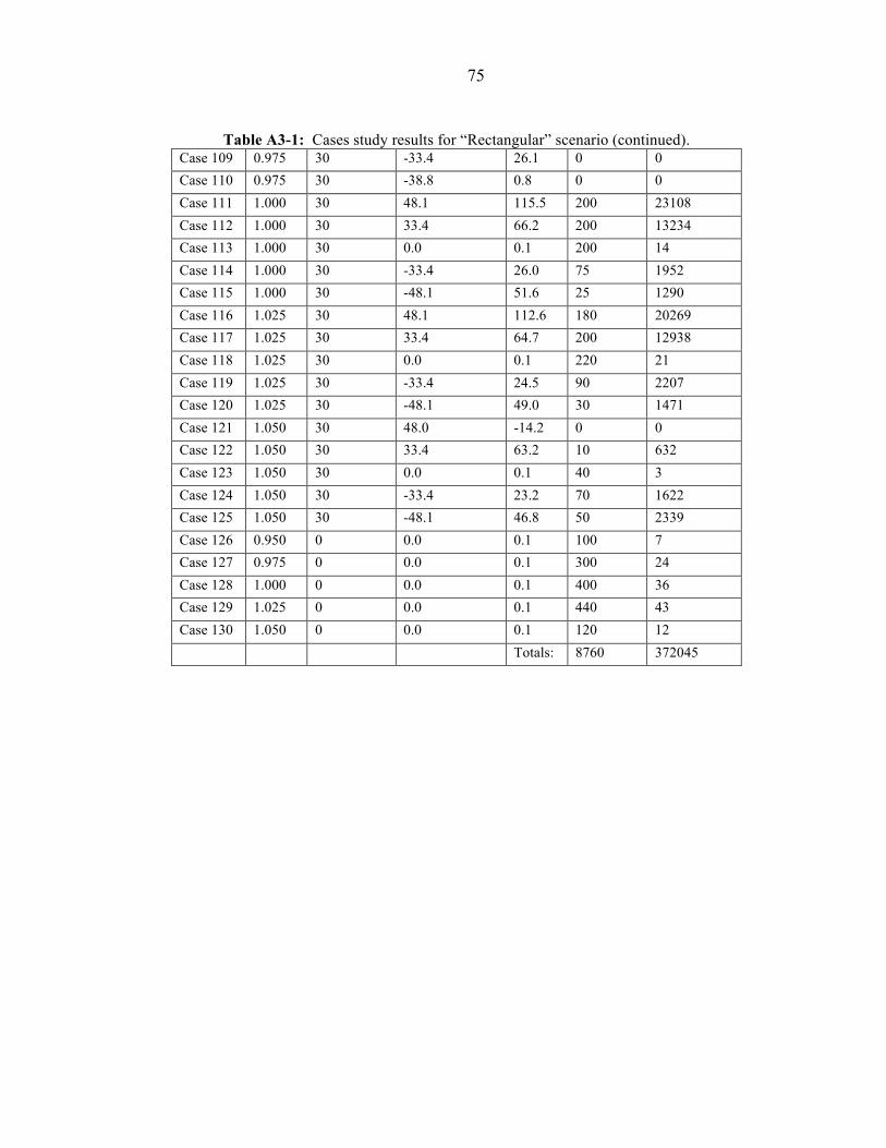
75
Table A3-1: Cases study results for “Rectangular” scenario (continued). Case 109 0.975 30 -33.4 26.1 0 0 Case 110 0.975 30 -38.8 0.8 0 0 Case 111 1.000 30 48.1 115.5 200 23108 Case 112 1.000 30 33.4 66.2 200 13234 Case 113 1.000 30 0.0 0.1 200 14 Case 114 1.000 30 -33.4 26.0 75 1952 Case 115 1.000 30 -48.1 51.6 25 1290 Case 116 1.025 30 48.1 112.6 180 20269 Case 117 1.025 30 33.4 64.7 200 12938 Case 118 1.025 30 0.0 0.1 220 21 Case 119 1.025 30 -33.4 24.5 90 2207 Case 120 1.025 30 -48.1 49.0 30 1471 Case 121 1.050 30 48.0 -14.2 0 0 Case 122 1.050 30 33.4 63.2 10 632 Case 123 1.050 30 0.0 0.1 40 3 Case 124 1.050 30 -33.4 23.2 70 1622 Case 125 1.050 30 -48.1 46.8 50 2339 Case 126 0.950 0 0.0 0.1 100 7 Case 127 0.975 0 0.0 0.1 300 24 Case 128 1.000 0 0.0 0.1 400 36 Case 129 1.025 0 0.0 0.1 440 43 Case 130 1.050 0 0.0 0.1 120 12 Totals: 8760 372045

76
Appendix 4 Case Study Results for the “Rectangular” Scenario with
Extended Voltage Range
Table A4-1: Cases study results for “Rectangular” scenario with extended voltage range.
POI Voltage (pu)
Real Power Generation (MW)
Reactive Power Generation (MVAr)
Savings (kW)
Frequency (hrs/year)
Savings per Year (kWhr)
Case 1 0.950 150 48.1 166.3 20 3325 Case 2 0.950 150 33.4 197.2 10 1972 Case 3 0.950 150 0.0 8.6 0 0 Case 4 0.950 150 -33.4 216.8 0 0 Case 5 0.950 150 -48.1 145.8 0 0 Case 6 0.975 150 48.1 156.8 40 6272 Case 7 0.975 150 33.4 187.3 20 3746 Case 8 0.975 150 0.0 7.3 10 73 Case 9 0.975 150 -33.4 211.2 0 0 Case 10 0.975 150 -48.1 354.0 0 0 Case 11 1.000 150 48.1 147.5 100 14751 Case 12 1.000 150 33.4 178.6 75 13391 Case 13 1.000 150 0.0 6.3 50 314 Case 14 1.000 150 -33.4 204.1 40 8165 Case 15 1.000 150 -48.1 347.3 10 3473 Case 16 1.025 150 48.1 124.3 100 12427 Case 17 1.025 150 33.4 154.3 100 15430 Case 18 1.025 150 0.0 5.5 250 1366 Case 19 1.025 150 -33.4 198.2 100 19820 Case 20 1.025 150 -48.1 342.3 50 17113 Case 21 1.050 150 48.1 -230.0 0 0 Case 22 1.050 150 33.4 38.4 0 0 Case 23 1.050 150 0.0 4.7 25 118 Case 24 1.050 150 -33.4 191.9 50 9596 Case 25 1.050 150 -48.1 335.1 50 16753 Case 26 0.950 120 48.1 348.0 20 6960 Case 27 0.950 120 33.4 192.6 10 1926 Case 28 0.950 120 0.0 3.5 0 0 Case 29 0.950 120 -33.4 216.9 0 0 Case 30 0.950 120 -48.1 148.5 0 0 Case 31 0.975 120 48.1 339.4 100 33936

77
Table A4-1: Cases study results for “Rectangular” scenario with extended voltage range (continued).
POI Voltage (pu)
Real Power Generation (MW)
Reactive Power Generation (MVAr)
Savings (kW)
Frequency (hrs/year)
Savings per Year (kWhr)
Case 32 0.975 120 33.4 184.2 30 5527 Case 33 0.975 120 0.0 3.0 10 30 Case 34 0.975 120 -33.4 209.1 0 0 Case 35 0.975 120 -48.1 359.9 0 0 Case 36 1.000 120 48.1 328.3 120 39394 Case 37 1.000 120 33.4 176.2 80 14096 Case 38 1.000 120 0.0 2.6 75 191 Case 39 1.000 120 -33.4 203.6 50 10181 Case 40 1.000 120 -48.1 350.9 15 5264 Case 41 1.025 120 48.1 282.2 120 33864 Case 42 1.025 120 33.4 167.5 135 22619 Case 43 1.025 120 0.0 2.2 200 436 Case 44 1.025 120 -33.4 197.4 80 15792 Case 45 1.025 120 -48.1 347.1 40 13883 Case 46 1.050 120 48.1 91.1 0 0 Case 47 1.050 120 33.4 132.7 15 1990 Case 48 1.050 120 0.0 1.8 50 92 Case 49 1.050 120 -33.4 190.5 100 19047 Case 50 1.050 120 -48.1 338.5 50 16925 Case 51 0.950 90 48.1 345.0 50 17249 Case 52 0.950 90 33.4 190.2 15 2853 Case 53 0.950 90 0.0 1.0 0 0 Case 54 0.950 90 -33.4 73.4 0 0 Case 55 0.950 90 -48.1 4.6 0 0 Case 56 0.975 90 48.1 336.4 110 37008 Case 57 0.975 90 33.4 183.0 50 9151 Case 58 0.975 90 0.0 0.9 10 9 Case 59 0.975 90 -33.4 210.2 0 0 Case 60 0.975 90 -48.1 364.8 0 0 Case 61 1.000 90 48.1 327.3 120 39271 Case 62 1.000 90 33.4 175.3 100 17533 Case 63 1.000 90 0.0 0.8 85 66 Case 64 1.000 90 -33.4 203.3 65 13216 Case 65 1.000 90 -48.1 357.5 30 10724 Case 66 1.025 90 48.1 317.5 150 47632

78
Table A4-1: Cases study results for “Rectangular” scenario with extended voltage range (continued).
POI Voltage (pu)
Real Power Generation (MW)
Reactive Power Generation (MVAr)
Savings (kW)
Frequency (hrs/year)
Savings per Year (kWhr)
Case 67 1.025 90 33.4 167.3 150 25088 Case 68 1.025 90 0.0 0.7 150 98 Case 69 1.025 90 -33.4 198.0 75 14852 Case 70 1.025 90 -48.1 350.8 30 10524 Case 71 1.050 90 48.1 120.0 20 2399 Case 72 1.050 90 33.4 158.8 35 5559 Case 73 1.050 90 0.0 0.5 45 23 Case 74 1.050 90 -33.4 190.4 70 13327 Case 75 1.050 90 -48.1 342.8 40 13711 Case 76 0.950 60 48.1 345.3 60 20718 Case 77 0.950 60 33.4 191.2 20 3825 Case 78 0.950 60 0.0 0.2 0 0 Case 79 0.950 60 -33.4 74.7 0 0 Case 80 0.950 60 -48.1 7.5 0 0 Case 81 0.975 60 48.1 336.7 120 40406 Case 82 0.975 60 33.4 184.0 100 18401 Case 83 0.975 60 0.0 0.1 15 2 Case 84 0.975 60 -33.4 212.0 0 0 Case 85 0.975 60 -48.1 151.9 0 0 Case 86 1.000 60 48.1 327.8 130 42610 Case 87 1.000 60 33.4 175.5 110 19301 Case 88 1.000 60 0.0 0.1 90 13 Case 89 1.000 60 -33.4 206.1 75 15458 Case 90 1.000 60 -48.1 363.4 40 14536 Case 91 1.025 60 48.1 318.5 100 31854 Case 92 1.025 60 33.4 167.7 200 33548 Case 93 1.025 60 0.0 0.1 200 22 Case 94 1.025 60 -33.4 198.9 100 19894 Case 95 1.025 60 -48.1 355.7 40 14229 Case 96 1.050 60 48.1 121.3 20 2426 Case 97 1.050 60 33.4 159.8 30 4794 Case 98 1.050 60 0.0 0.1 60 6 Case 99 1.050 60 -33.4 191.8 60 11510 Case 100 1.050 60 -48.1 348.3 30 10449 Case 101 0.950 30 48.1 346.9 80 27752

79
Table A4-1: Cases study results for “Rectangular” scenario with extended voltage range (continued).
POI Voltage (pu)
Real Power Generation (MW)
Reactive Power Generation (MVAr)
Savings (kW)
Frequency (hrs/year)
Savings per Year (kWhr)
Case 102 0.950 30 33.4 192.9 10 1929 Case 103 0.950 30 0.0 0.1 0 0 Case 104 0.950 30 -33.4 76.0 0 0 Case 105 0.950 30 -48.1 1.3 0 0 Case 106 0.975 30 48.1 338.4 150 50756 Case 107 0.975 30 33.4 185.6 125 23203 Case 108 0.975 30 0.0 0.0 45 2 Case 109 0.975 30 -33.4 214.7 0 0 Case 110 0.975 30 -48.1 156.0 0 0 Case 111 1.000 30 48.1 329.7 200 65933 Case 112 1.000 30 33.4 177.2 200 35442 Case 113 1.000 30 0.0 0.1 200 14 Case 114 1.000 30 -33.4 207.0 75 15524 Case 115 1.000 30 -48.1 369.5 25 9237 Case 116 1.025 30 48.1 320.8 180 57747 Case 117 1.025 30 33.4 169.7 200 33948 Case 118 1.025 30 0.0 0.1 220 21 Case 119 1.025 30 -33.4 200.5 90 18049 Case 120 1.025 30 -48.1 360.7 30 10822 Case 121 1.050 30 48.1 311.8 0 0 Case 122 1.050 30 33.4 162.1 10 1621 Case 123 1.050 30 0.0 0.1 40 3 Case 124 1.050 30 -33.4 192.7 70 13490 Case 125 1.050 30 -48.1 352.1 50 17605 Case 126 0.950 0 0.0 0.1 100 7 Case 127 0.975 0 0.0 0.1 300 24 Case 128 1.000 0 0.0 0.1 400 36 Case 129 1.025 0 0.0 0.1 440 43 Case 130 1.050 0 0.0 0.1 120 12 Totals: 8760 1357770
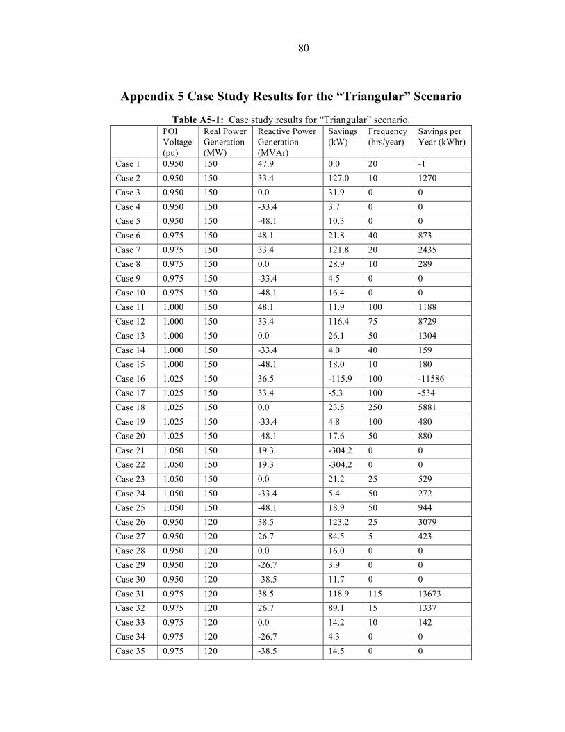
80
Appendix 5 Case Study Results for the “Triangular” Scenario
Table A5-1: Case study results for “Triangular” scenario. POI
Voltage (pu)
Real Power Generation (MW)
Reactive Power Generation (MVAr)
Savings (kW)
Frequency (hrs/year)
Savings per Year (kWhr)
Case 1 0.950 150 47.9 0.0 20 -1 Case 2 0.950 150 33.4 127.0 10 1270 Case 3 0.950 150 0.0 31.9 0 0 Case 4 0.950 150 -33.4 3.7 0 0 Case 5 0.950 150 -48.1 10.3 0 0 Case 6 0.975 150 48.1 21.8 40 873 Case 7 0.975 150 33.4 121.8 20 2435 Case 8 0.975 150 0.0 28.9 10 289 Case 9 0.975 150 -33.4 4.5 0 0 Case 10 0.975 150 -48.1 16.4 0 0 Case 11 1.000 150 48.1 11.9 100 1188 Case 12 1.000 150 33.4 116.4 75 8729 Case 13 1.000 150 0.0 26.1 50 1304 Case 14 1.000 150 -33.4 4.0 40 159 Case 15 1.000 150 -48.1 18.0 10 180 Case 16 1.025 150 36.5 -115.9 100 -11586 Case 17 1.025 150 33.4 -5.3 100 -534 Case 18 1.025 150 0.0 23.5 250 5881 Case 19 1.025 150 -33.4 4.8 100 480 Case 20 1.025 150 -48.1 17.6 50 880 Case 21 1.050 150 19.3 -304.2 0 0 Case 22 1.050 150 19.3 -304.2 0 0 Case 23 1.050 150 0.0 21.2 25 529 Case 24 1.050 150 -33.4 5.4 50 272 Case 25 1.050 150 -48.1 18.9 50 944 Case 26 0.950 120 38.5 123.2 25 3079 Case 27 0.950 120 26.7 84.5 5 423 Case 28 0.950 120 0.0 16.0 0 0 Case 29 0.950 120 -26.7 3.9 0 0 Case 30 0.950 120 -38.5 11.7 0 0 Case 31 0.975 120 38.5 118.9 115 13673 Case 32 0.975 120 26.7 89.1 15 1337 Case 33 0.975 120 0.0 14.2 10 142 Case 34 0.975 120 -26.7 4.3 0 0 Case 35 0.975 120 -38.5 14.5 0 0

81
Table A5-1: Case study results for “Triangular” scenario (continued). POI
Voltage (pu)
Real Power Generation (MW)
Reactive Power Generation (MVAr)
Savings (kW)
Frequency (hrs/year)
Savings per Year (kWhr)
Case 36 1.000 120 38.5 114.0 160 18241 Case 37 1.000 120 26.7 77.1 40 3083 Case 38 1.000 120 0.0 12.5 75 935 Case 39 1.000 120 -26.7 4.3 30 130 Case 40 1.000 120 -38.5 15.1 35 527 Case 41 1.025 120 38.5 108.3 180 19500 Case 42 1.025 120 26.7 73.4 75 5505 Case 43 1.025 120 0.0 10.8 200 2165 Case 44 1.025 120 -26.7 5.0 80 399 Case 45 1.025 120 -38.5 15.0 40 602 Case 46 1.050 120 28.5 -255.4 0 0 Case 47 1.050 120 26.7 -84.2 15 -1263 Case 48 1.050 120 0.0 9.3 50 463 Case 49 1.050 120 -26.7 5.2 100 517 Case 50 1.050 120 -38.5 14.5 50 723 Case 51 0.950 90 28.9 28.8 50 1438 Case 52 0.950 90 20.0 16.4 15 246 Case 53 0.950 90 0.0 1.0 0 0 Case 54 0.950 90 -20.0 4.4 0 0 Case 55 0.950 90 -28.9 10.3 0 0 Case 56 0.975 90 28.9 26.4 110 2902 Case 57 0.975 90 20.0 15.3 50 763 Case 58 0.975 90 0.0 0.9 10 9 Case 59 0.975 90 -20.0 4.3 0 0 Case 60 0.975 90 -28.9 11.2 0 0 Case 61 1.000 90 28.9 24.7 120 2970 Case 62 1.000 90 20.0 14.0 100 1405 Case 63 1.000 90 0.0 0.8 85 66 Case 64 1.000 90 -20.0 4.5 35 157 Case 65 1.000 90 -28.9 11.0 60 658 Case 66 1.025 90 28.9 23.8 150 3570 Case 67 1.025 90 20.0 12.7 150 1912 Case 68 1.025 90 0.0 0.7 150 98 Case 69 1.025 90 -20.0 4.2 50 208 Case 70 1.025 90 -28.9 11.1 55 613 Case 71 1.050 90 28.9 7.4 20 149 Case 72 1.050 90 20.0 12.0 35 418

82
Table A5-1: Case study results for “Triangular” scenario (continued). POI
Voltage (pu)
Real Power Generation (MW)
Reactive Power Generation (MVAr)
Savings (kW)
Frequency (hrs/year)
Savings per Year (kWhr)
Case 73 1.050 90 0.0 0.6 45 25 Case 74 1.050 90 -20.0 4.1 35 143 Case 75 1.050 90 -28.9 10.6 75 792 Case 76 0.950 60 19.2 36.7 80 2936 Case 77 0.950 60 13.4 23.0 10 230 Case 78 0.950 60 0.0 0.2 0 0 Case 79 0.950 60 -13.4 3.0 0 0 Case 80 0.950 60 -19.2 6.7 0 0 Case 81 0.975 60 19.2 35.2 170 5981 Case 82 0.975 60 13.4 21.7 50 1086 Case 83 0.975 60 0.0 0.1 15 2 Case 84 0.975 60 -13.4 2.5 0 0 Case 85 0.975 60 -19.2 6.7 0 0 Case 86 1.000 60 19.2 33.7 190 6397 Case 87 1.000 60 13.4 20.5 50 1025 Case 88 1.000 60 0.0 0.1 90 13 Case 89 1.000 60 -13.4 2.8 40 111 Case 90 1.000 60 -19.2 6.0 75 453 Case 91 1.025 60 19.2 32.7 200 6546 Case 92 1.025 60 13.4 19.7 100 1967 Case 93 1.025 60 0.0 0.1 200 22 Case 94 1.025 60 -13.4 2.5 40 101 Case 95 1.025 60 -19.2 6.2 90 560 Case 96 1.050 60 19.2 31.2 35 1093 Case 97 1.050 60 13.4 18.8 15 282 Case 98 1.050 60 0.0 0.1 60 6 Case 99 1.050 60 -13.4 2.3 30 70 Case 100 1.050 60 -19.2 5.8 60 346 Case 101 0.950 30 9.6 9.8 80 784 Case 102 0.950 30 6.7 4.5 10 45 Case 103 0.950 30 0.0 0.1 0 0 Case 104 0.950 30 -6.7 1.1 0 0 Case 105 0.950 30 -9.6 2.4 0 0 Case 106 0.975 30 9.6 9.0 225 2033 Case 107 0.975 30 6.7 3.8 50 190 Case 108 0.975 30 0.0 0.0 45 2 Case 109 0.975 30 -6.7 1.3 0 0
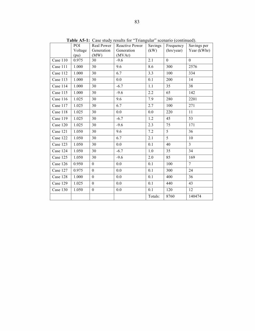
83
Table A5-1: Case study results for “Triangular” scenario (continued). POI
Voltage (pu)
Real Power Generation (MW)
Reactive Power Generation (MVAr)
Savings (kW)
Frequency (hrs/year)
Savings per Year (kWhr)
Case 110 0.975 30 -9.6 2.1 0 0 Case 111 1.000 30 9.6 8.6 300 2576 Case 112 1.000 30 6.7 3.3 100 334 Case 113 1.000 30 0.0 0.1 200 14 Case 114 1.000 30 -6.7 1.1 35 38 Case 115 1.000 30 -9.6 2.2 65 142 Case 116 1.025 30 9.6 7.9 280 2201 Case 117 1.025 30 6.7 2.7 100 271 Case 118 1.025 30 0.0 0.0 220 11 Case 119 1.025 30 -6.7 1.2 45 53 Case 120 1.025 30 -9.6 2.3 75 171 Case 121 1.050 30 9.6 7.2 5 36 Case 122 1.050 30 6.7 2.1 5 10 Case 123 1.050 30 0.0 0.1 40 3 Case 124 1.050 30 -6.7 1.0 35 34 Case 125 1.050 30 -9.6 2.0 85 169 Case 126 0.950 0 0.0 0.1 100 7 Case 127 0.975 0 0.0 0.1 300 24 Case 128 1.000 0 0.0 0.1 400 36 Case 129 1.025 0 0.0 0.1 440 43 Case 130 1.050 0 0.0 0.1 120 12 Totals: 8760 140474

84
Appendix 6 Case Study Results for the “Triangular” Scenario with
Extended Voltage Range
Table A6-1: Case study results for “Triangular” scenario with extended voltage range
POI Voltage (pu)
Real Power Generation (MW)
Reactive Power Generation (MVAr)
Savings (kW)
Frequency (hrs/year)
Savings per Year (kWhr)
Case 1 0.950 150 48.1 166.3 20 3325 Case 2 0.950 150 33.4 197.2 10 1972 Case 3 0.950 150 0.0 8.5 0 0 Case 4 0.950 150 -33.4 3.7 0 0 Case 5 0.950 150 -48.1 10.9 0 0 Case 6 0.975 150 48.1 156.8 40 6272 Case 7 0.975 150 33.4 187.3 20 3746 Case 8 0.975 150 0.0 7.3 10 73 Case 9 0.975 150 -33.4 4.5 0 0 Case 10 0.975 150 -48.1 16.4 0 0 Case 11 1.000 150 48.1 147.5 100 14752 Case 12 1.000 150 33.4 177.6 75 13317 Case 13 1.000 150 0.0 6.3 50 314 Case 14 1.000 150 -33.4 4.0 40 159 Case 15 1.000 150 -48.1 18.0 10 180 Case 16 1.025 150 48.1 123.9 100 12388 Case 17 1.025 150 33.4 154.3 100 15430 Case 18 1.025 150 0.0 5.4 250 1352 Case 19 1.025 150 -33.4 4.8 100 480 Case 20 1.025 150 -48.1 17.6 50 880 Case 21 1.050 150 48.1 -230.3 0 0 Case 22 1.050 150 33.4 38.2 0 0 Case 23 1.050 150 0.0 4.7 25 116 Case 24 1.050 150 -33.4 5.4 50 272 Case 25 1.050 150 -48.1 18.9 50 944 Case 26 0.950 120 38.5 246.2 25 6156 Case 27 0.950 120 26.7 124.4 5 622 Case 28 0.950 120 0.0 3.5 0 0 Case 29 0.950 120 -26.7 5.0 0 0 Case 30 0.950 120 -38.5 11.7 0 0 Case 31 0.975 120 38.5 236.4 115 27190

85
Table A6-1: Case study results for “Triangular” scenario with extended voltage range (continued).
POI Voltage (pu)
Real Power Generation (MW)
Reactive Power Generation (MVAr)
Savings (kW)
Frequency (hrs/year)
Savings per Year (kWhr)
Case 32 0.975 120 26.7 116.3 15 1745 Case 33 0.975 120 0.0 3.0 10 30 Case 34 0.975 120 -26.7 4.3 0 0 Case 35 0.975 120 -38.5 14.5 0 0 Case 36 1.000 120 38.5 227.1 160 36342 Case 37 1.000 120 26.7 108.5 40 4342 Case 38 1.000 120 0.0 2.6 75 191 Case 39 1.000 120 -26.7 4.3 30 130 Case 40 1.000 120 -38.5 15.1 35 527 Case 41 1.025 120 38.5 218.3 180 39297 Case 42 1.025 120 26.7 100.3 75 7522 Case 43 1.025 120 0.0 2.2 200 436 Case 44 1.025 120 -26.7 5.0 80 399 Case 45 1.025 120 -38.5 15.0 40 602 Case 46 1.050 120 38.5 70.2 0 0 Case 47 1.050 120 26.7 84.2 15 1263 Case 48 1.050 120 0.0 1.9 50 94 Case 49 1.050 120 -26.7 5.2 100 517 Case 50 1.050 120 -38.5 15.9 50 793 Case 51 0.950 90 28.9 145.3 50 7265 Case 52 0.950 90 20.0 63.8 15 957 Case 53 0.950 90 0.0 1.0 0 0 Case 54 0.950 90 -20.0 4.4 0 0 Case 55 0.950 90 -28.9 10.3 0 0 Case 56 0.975 90 28.9 138.2 110 15200 Case 57 0.975 90 20.0 61.3 50 3063 Case 58 0.975 90 0.0 0.9 10 9 Case 59 0.975 90 -20.0 4.3 0 0 Case 60 0.975 90 -28.9 11.2 0 0 Case 61 1.000 90 28.9 130.6 120 15675 Case 62 1.000 90 20.0 58.5 100 5854 Case 63 1.000 90 0.0 0.8 85 66 Case 64 1.000 90 -20.0 4.5 35 157 Case 65 1.000 90 -28.9 11.0 60 658 Case 66 1.025 90 28.9 122.7 150 18408 Case 67 1.025 90 20.0 55.7 150 8354

86
Table A6-1: Case study results for “Triangular” scenario with extended voltage range (continued).
POI Voltage (pu)
Real Power Generation (MW)
Reactive Power Generation (MVAr)
Savings (kW)
Frequency (hrs/year)
Savings per Year (kWhr)
Case 68 1.025 90 0.0 0.7 150 98 Case 69 1.025 90 -20.0 4.2 50 208 Case 70 1.025 90 -28.9 11.1 55 613 Case 71 1.050 90 28.9 114.5 20 2290 Case 72 1.050 90 20.0 53.3 35 1865 Case 73 1.050 90 0.0 0.6 45 25 Case 74 1.050 90 -20.0 4.1 35 143 Case 75 1.050 90 -28.9 10.6 75 792 Case 76 0.950 60 19.2 58.4 80 4669 Case 77 0.950 60 13.4 28.6 10 286 Case 78 0.950 60 0.0 0.2 0 0 Case 79 0.950 60 -13.4 3.0 0 0 Case 80 0.950 60 -13.4 41.9 0 0 Case 81 0.975 60 19.2 56.0 170 9514 Case 82 0.975 60 13.4 26.4 50 1322 Case 83 0.975 60 0.0 0.1 15 2 Case 84 0.975 60 -13.4 3.1 0 0 Case 85 0.975 60 -13.4 40.2 0 0 Case 86 1.000 60 19.2 53.5 190 10166 Case 87 1.000 60 13.4 24.2 50 1212 Case 88 1.000 60 0.0 0.1 90 13 Case 89 1.000 60 -13.4 2.8 40 111 Case 90 1.000 60 -13.4 38.0 75 2847 Case 91 1.025 60 19.2 51.0 200 10198 Case 92 1.025 60 13.4 22.4 100 2237 Case 93 1.025 60 0.0 0.1 200 22 Case 94 1.025 60 -13.4 2.5 40 101 Case 95 1.025 60 -13.4 36.7 90 3304 Case 96 1.050 60 19.2 49.0 35 1714 Case 97 1.050 60 13.4 20.4 15 307 Case 98 1.050 60 0.0 0.1 60 6 Case 99 1.050 60 -13.4 2.8 30 85 Case 100 1.050 60 -13.4 34.9 60 2095 Case 101 0.950 30 9.6 2.3 80 185 Case 102 0.950 30 6.7 1.2 10 12 Case 103 0.950 30 0.0 0.1 0 0

87
Table A6-1: Case study results for “Triangular” scenario with extended voltage range (continued).
POI Voltage (pu)
Real Power Generation (MW)
Reactive Power Generation (MVAr)
Savings (kW)
Frequency (hrs/year)
Savings per Year (kWhr)
Case 104 0.950 30 -6.7 1.1 0 0 Case 105 0.950 30 -9.6 2.4 0 0 Case 106 0.975 30 9.6 2.1 225 461 Case 107 0.975 30 6.7 1.0 50 52 Case 108 0.975 30 0.0 0.1 45 4 Case 109 0.975 30 -6.7 1.0 0 0 Case 110 0.975 30 -9.6 2.1 0 0 Case 111 1.000 30 9.6 2.1 300 628 Case 112 1.000 30 6.7 0.9 100 90 Case 113 1.000 30 0.0 0.1 200 14 Case 114 1.000 30 -6.7 1.1 35 38 Case 115 1.000 30 -9.6 2.2 65 142 Case 116 1.025 30 9.6 1.9 280 522 Case 117 1.025 30 6.7 0.9 100 94 Case 118 1.025 30 0.0 0.0 220 11 Case 119 1.025 30 -6.7 1.2 45 53 Case 120 1.025 30 -9.6 2.3 75 171 Case 121 1.050 30 9.6 1.7 5 8 Case 122 1.050 30 6.7 0.8 5 4 Case 123 1.050 30 0.0 0.1 40 3 Case 124 1.050 30 -6.7 1.0 35 34 Case 125 1.050 30 -9.6 2.0 85 169 Case 126 0.950 0 0.0 0.1 100 11 Case 127 0.975 0 0.0 0.1 300 24 Case 128 1.000 0 0.0 0.1 400 36 Case 129 1.025 0 0.0 0.1 440 43 Case 130 1.050 0 0.0 0.1 120 12 Totals: 8760 338897