central valley hydrology study - ford...

Central Valley hydrology study

November 29, 2015

Prepared for California Department of Water Resources Letter of agreement #4600007762

Prepared by US Army Corps of Engineers Sacramento District and David Ford Consulting Engineers, Inc.

3

Contents Expectations of use .............................................................................. 7

Purpose of the hydrology .................................................................... 7 Responsibility of users ....................................................................... 7 Basic assumptions and limitations ........................................................ 7

Executive summary ............................................................................ 10 Situation ........................................................................................ 10 Analysis overview ............................................................................ 10

Requirements .............................................................................. 10 Procedure overview ...................................................................... 11

Analysis review and oversight ........................................................... 12 Results .......................................................................................... 12

Introduction ...................................................................................... 13 Authority ........................................................................................ 13 Watershed description ...................................................................... 13 Sacramento and San Joaquin river basin flood control system ................ 16 Motivation of current DWR studies of the watershed ............................. 17 Hydrology study .............................................................................. 19 Study requirements ......................................................................... 20 Potential effects of climate change on study results .............................. 20 Purpose of documentation ................................................................ 20 Approval and certification ................................................................. 20 Relevant documents ........................................................................ 20

Comparison to previous watershed study ............................................... 21

Watershed description......................................................................... 27 Sacramento River basin ................................................................... 27

Basin characteristics ..................................................................... 27 Hydrography ............................................................................... 28 Topography ................................................................................. 29 Soils 29 Vegetation .................................................................................. 29 Climate ....................................................................................... 29 Temperature ............................................................................... 30 Precipitation ................................................................................ 30 Snowpack ................................................................................... 31

San Joaquin River basin ................................................................... 31 Basin characteristics ..................................................................... 31 Hydrography ............................................................................... 32 Topography ................................................................................. 32 Soils 33 Vegetation .................................................................................. 33 Climate ....................................................................................... 33 Temperatures .............................................................................. 33 Precipitation ................................................................................ 34 Snowpack ................................................................................... 35

Analysis procedure ............................................................................. 36

4

Overview of procedure ..................................................................... 36 Mixed population analysis and integration into the CVHS ....................... 39

Mixed population analysis .............................................................. 39 Separation of events to create the time series .................................. 40

Regional skew and its use in CVHS ..................................................... 40 Term “unregulated flow” and its use in CVHS ...................................... 45

Study products and applications ........................................................... 48 Study products ............................................................................... 48 First application regulated condition products ...................................... 48 Application of study products ............................................................ 49

Unregulated flow time series development ............................................. 54 Estimate daily reservoir inflow ........................................................... 54

Situation ..................................................................................... 54 Pertinent guidance and discussion .................................................. 54 Study procedure .......................................................................... 57

Estimation of ungaged local flows ...................................................... 57 Situation ..................................................................................... 57 Pertinent guidance and discussion .................................................. 58 Study procedure .......................................................................... 59

Application and distribution of local flow ............................................. 59 Situation ..................................................................................... 59 Pertinent guidance and discussion .................................................. 59 Study procedure .......................................................................... 60

Approach for extending data or filling in gaps ...................................... 60 Situation ..................................................................................... 60 Pertinent guidance and discussion .................................................. 61 Description of methods to support flow-frequency analysis ................. 61 Methods to support assessing the effects of regulation....................... 62 Study procedure .......................................................................... 62

Smooth unregulated flow time series .................................................. 62 Situation ..................................................................................... 62 Pertinent guidance and discussion .................................................. 62 Study procedure .......................................................................... 63

Procedures for routing unregulated flows through the system ................ 63 Situation ..................................................................................... 63 Pertinent guidance and discussion .................................................. 63 Study procedure .......................................................................... 65

Unregulated frequency analysis ............................................................ 66 Separation of seasonal data .............................................................. 68


Identify annual maximum series ........................................................ 69 Situation ..................................................................................... 69 Pertinent guidance and discussion .................................................. 69

Study procedure ............................................................................. 70 Calculate regional skew values .......................................................... 70

Situation ..................................................................................... 70

5

Pertinent guidance and discussion .................................................. 70 Study procedure .......................................................................... 70

Fit frequency curves ........................................................................ 71 Situation ..................................................................................... 71 Pertinent guidance and discussion .................................................. 71 Study procedure .......................................................................... 71

Review and adopt curves .................................................................. 72 Situation ..................................................................................... 72 Pertinent guidance and discussion .................................................. 72 Study procedure .......................................................................... 72

Regulated flow time series development for specified regulated condition ........................................................................................ 74 Definition of reservoir operation criteria .............................................. 74


Definition of initial conditions in flood control reservoirs ........................ 79 Situation ..................................................................................... 79 Pertinent guidance and discussion .................................................. 79 Study procedure .......................................................................... 79

Representation of headwater reservoirs and distribution of historical flows in reservoir simulation model ................................. 80


Initial conditions for reservoir simulation-headwater reservoirs .............. 83 Situation ..................................................................................... 83 Pertinent guidance and discussion .................................................. 84 Study procedure .......................................................................... 84

Identify and scale historical floods-of-record ....................................... 86 Situation ..................................................................................... 86 Pertinent guidance and discussion .................................................. 86 Study procedure .......................................................................... 87

Simulate reservoir operations for historical and scaled floods ................. 89 Route reservoir releases through the regulated system ......................... 89

Situation ..................................................................................... 89 Pertinent guidance and discussion .................................................. 89 Top of Levee Modification for HEC-RAS ............................................ 90 Study procedure .......................................................................... 90

Development and application of unregulated-regulated flow transform ....................................................................................... 91 Identification of critical duration at analysis points ............................... 91

Situation ..................................................................................... 91 Pertinent guidance and discussion .................................................. 91 For completely unregulated watersheds the critical duration

assessment is not required as there is no difference between the unregulated and regulated flow hydrographs. ...................................................................... 93

Study procedure .......................................................................... 93

6

Fitting a “most likely” transform through the datasets .......................... 93 Situation ..................................................................................... 93 Pertinent guidance and discussion .................................................. 93 Study procedure .......................................................................... 94

Results ............................................................................................. 96

Lessons learned and cautionary notes ................................................... 97

Future work ...................................................................................... 100

References ....................................................................................... 102

Glossary .......................................................................................... 104

Supplemental resources ..................................................................... 107

Contributors to study ......................................................................... 109 Study team ................................................................................... 109 Study review team ......................................................................... 110 Acknowledgements ......................................................................... 110

Appendix I. Analysis points ................................................................. 111

Appendix II. Summary of computer model development and uses ............ 112

Appendix III. Flow time series development and documentation ............... 113

Appendix IV. Completed unregulated flow time series ............................. 114

Appendix V. Annual maximum series for frequency analysis .................... 115

Appendix VI. Unregulated flow-frequency analysis ................................. 116

Appendix VII. Unregulated flow-frequency curves .................................. 117

Appendix VIII. Completed regulated flow times series ............................ 118

Appendix IX. Extracted event dataset ................................................... 119

Appendix X: Development and application of unregulated-regulated flow transform ................................................................. 120

Appendix XI. Rainfall-runoff modeling .................................................. 121

7

Expectations of use Purpose of the hydrology

The intent of the hydrology developed for the Central Valley hydrology study is to provide a basis for defining existing hydrologic conditions at selected locations in the watershed. Specifically, these locations were selected to assess the Federal-state levee system.

Specifically developed to support this particular study, the hydrology may or may not fulfill the technical requirements of site-specific investigations within the Central Valley where CVHS analysis points are not located. This includes both the unregulated flow-frequency analysis and the regulated condition analysis. Further, this study has evaluated the effects of various spatial and temporal distributions of storms. Care should be taken on relying on a single spatial and temporal distribution given the size and regulating features of the watershed.

Prior to its use, the size and scope of each study, even at the pre-feasibility level, will need to be evaluated to determine if the hydrology can be directly applied, with specific focus on the regulated conditions and where frequency analysis is required.

Hydrologic analyses performed for such a large spatial area and at the level of detail documented herein present challenges and opportunities unique to such ambitious studies. The Central Valley hydrology study has made possible a system-wide update of the Central Valley unregulated flow hydrology and an overall modernization of the models used by Sacramento District hydrologists and engineers.

Responsibility of users The points of contact for comments and feedback are:

Mr. John High, District Hydrologist U.S. Army Corps of Engineers Sacramento District (916) 557-7136

Mr. Brad Moore, PE, CVHS Technical Lead U.S. Army Corps of Engineers Sacramento District (916) 557-7114

The complexity and intricacy in the development of the hydrology of this study require that it be used only by qualified hydrologic/hydraulic engineers and scientists familiar with proper applications of hydrologic products. Professional expertise and judgment should be exercised for all analyses conducted using this hydrology.

Basic assumptions and limitations The hydrology, as presented herein, was created to support flood management and evaluation activities.

8

The models developed for the Central Valley hydrology study analysis were created with the following assumptions and limitations:

1. The data are stationary: the statistical properties of the forcing hydrologic and climatic conditions are unchanging with time. The potential effect of climate change on the curves is addressed independently.

2. Unregulated system inflows, boundary conditions, are based on daily values, but the model simulation times may have smaller time steps.

3. The unregulated flow frequency curves are strictly rainflood frequency curves. Snowmelt runoff is not directly incorporated into the analysis.

4. Unregulated flow frequency curves were designed to quantify the total flows that the basins produced in rainfloods.

5. Underlying unregulated flow time series and thus the volume-frequency curves have been developed for the purposes of flood flow analysis. They may not be appropriate for low flow or environmental analysis purposes.

6. Flow hydrographs are predicated on flood runoff from historical events, not precipitation. The approach was driven entirely by historical flow data; precipitation never entered into any portion of the methodology. [The exception here is for the few analysis points where flow frequency curves were derived from rainfall-runoff models using design precipitation events. These cases are specifically noted in the documentation.]

7. Flows in the unregulated system channel routing models are constrained to the channel, thus the effects of floodplain storage within the leveed system are removed.

8. Scaled historical events are used to stress the system and simulate events rarer than those observed in the CVHS study area. However, these events are only used for the transform development. For the unregulated flow-frequency analysis, only the historical record was used.

Selected historical-event flows and patterns for scaling and simulation of system performance represent the most likely spatial and temporal distributions associated with future large system events. The regulated flow time series developed, and thus the resulting unregulated flow to regulated flow transforms, are also based on a specific set of assumptions. These assumptions are described in this report. Most notably, as related to regulated flow delivery in the system, are:

1. Reservoir operations for headwater reservoirs (non-project reservoirs) are based on a specific set of assumptions as documented in the technical appendices.

9

2. Reservoir operations for project reservoirs follow operating rules specified in each reservoirs respective water control manual, and only the dedicated flood pool is used for storing water. Given that this study focuses on flood management, the reservoir models are configured with flood management rules only. Water supply operation and minimum flow requirements are not a focus within the reservoir simulation models. Starting storages at headwater dams were coordinated with FEMA in order to validate those assumptions would be acceptable for mapping FEMA floodplains. Other modeling assumptions, such as were utilized in the CVHS HEC-RAS models do not necessarily meet FEMA guidelines.

3. Levees along the channel model are allowed to overtop and water can be stored in the floodplain, but the levees do not fail.

4. Flow splits at bifurcations and system weirs are as represented in the channel routing model described herein.

These regulated flow routing assumptions may or may not be consistent with a specific future study need or application.

10

Executive summary Situation

In late 2007, the California Department of Water Resources (DWR) estimated that 1.8 million Californians (5% of the State’s population) lived in the so-called 100-year floodplain (DWR 2007). DWR further estimated that almost 10% of residents of California’s Central Valley live or work in the 200-year floodplain (DWR 2007). A growing Californian population will increase this vulnerability to flooding, with more people and property moving into potentially inundated areas. A changing climate may expand the areas subject to inundation at a given risk level and may envelop more land and more people.

The flood control system that protects Californians in the Central Valley is aging and the information upon which floodplain management decisions must be made is incomplete or out of date.

In response to these concerns, in 2007 the state initiated the FloodSAFE California program, which aims to increase flood protection and improve flood preparedness and response. For the state to achieve its FloodSAFE goals, the data upon which it depends must be updated.

In support of these efforts, DWR has delegated to us, the US Army Corps of Engineers, Sacramento District (Corps), the task of completing a hydrologic analysis of the Sacramento and San Joaquin river basins. This hydrologic analysis will be used to support the assessment of the current federal-state levee protection system.

Analysis overview The goal of the hydrologic analysis is to develop the required frequency curves, which provide estimates of the annual exceedence probability of flows, to support DWR’s floodplain mapping effort. These curves are required at analysis points—locations at which frequency curves must be developed—to facilitate floodplain mapping of all areas protected by the federal-state levee system in the basin. These points must be of sufficient spatial resolution to map accurately the floodplain in accordance with current standards of practice. Floodplain maps will be developed for annual exceedence probabilities ranging from 0.10 (10-year) to 0.002 (500-year).

Requirements

The primary requirements of this hydrologic analysis include:

Yielding sufficient resolution to permit DWR to prepare floodplain maps of areas protected by federal-state levees in the basin.

Meeting requirements of the Federal Emergency Management Agency’s National Flood Insurance Program.

Being consistent with the standard of practice, using well established, peer-reviewed, accepted procedures and methods.

11

The secondary requirements of this hydrologic analysis include:

Using procedures that can be reproduced at a later time to update the frequency curves.

Acknowledging and describing the uncertainty in the hydrologic results.

Facilitating follow-up analyses, such as evaluating the effect of climate change on the areas subject to inundation at a given risk level. This may include use of models or procedures that can be adjusted or modified to assess possible changes to the frequency curves.

Procedure overview

To develop required frequency curves for floodplain mapping along and behind federal-state levees throughout the Sacramento-San Joaquin river basin, we will complete a floods-of-record analysis. To develop the required frequency curves, we will:

1. Process historic data to remove the effects of system regulation and develop a time series of unregulated flows at each of the required points. Follow consistent methods in fitting the frequency curve with the unregulated time series. This is illustrated in Figure 1(a).

2. Using the historic records, a reservoir operation simulation model, and an unsteady flow hydraulic model of the system, develop an unregulated-regulated flow transform curve for each analysis point. This curve is illustrated in Figure 1(b).

3. Combine the results from step 1 and step 2 to develop a regulated flow-frequency curve for each analysis point.

4. Using an unsteady flow hydraulic model to simulate the floods of record, develop a relationship between event peak flow and stage for each analysis point. This curve is illustrated in Figure 1(c). This relationship captures the effect of downstream control and the timing of flows at confluences.

5. Combine the curves developed above to obtain a stage-frequency curve for each analysis point. This curve is illustrated in Figure 1(d).

Thus, at the completion of the analysis, we will have curves a, b, and c, and the ability to create d, in Figure 1 for each analysis point. These can then be used as input to the hydraulic analysis to develop floodplain maps. As needed, additional frequency analyses can be completed on the simulated record length to develop volume-frequency curves.

The chapters following describe these steps in more detail.

12

Figure 1. Overview of hydrologic analysis procedure

Analysis review and oversight The project team included Corps staff, DWR staff, USGS staff, and consultants to these agencies. In addition, to the project team, various review teams were also developed. The review teams included representatives from DWR, DWR consultants that are developing hydraulic models of the system, specialists in flood hydrology, and the Hydrologic Engineering Center (HEC) of the Corps.

To facilitate the review, we prepared analysis plans and documentation of the proposed procedures to gain wide concurrence and understanding for the study. These materials were provided to the review team above. In addition, supplemental material was provided and distributed to expand on various study details as well as establishment of a Web forum (www.cvhydrology.org.)

Results This document describes the results. The final products are frequency curves and analysis of 1 regulated condition. These final products are available at the study site: www.cvhydrology.org. User name: CVHS_GEN and password: featherriver.

(d)

(c) (b) (a) Unregulated flow

Regu

late

d flo

w

Flow

Stag

e

Probability U

nreg

ulat

ed fl

ow

Probability St

age

13

Introduction Authority

This study was completed under the authority of Letter of Agreement 4600007762 between USACE and DWR.

Watershed description The Sacramento and San Joaquin river basins, also known as California’s Central Valley, cover approximately 3/8 of the state. The basin is illustrated in Figure 2. Below we provided a brief description of the watershed and the hydrologic conditions. Detailed descriptions are available in the Sacramento and San Joaquin river basins comprehensive study interim report (USACE 2002a).

The Sacramento River watershed includes approximately 27,000 square miles upstream of Rio Vista, CA. The basin is 240 miles long and up to 150 miles wide. It is bounded by the Sierra Nevada on the east, the Coast Range on the west, the Cascade Range and Trinity Mountains on the north, and the Sacramento–San Joaquin Delta on the south. Major tributaries to the Sacramento River include the Feather and American rivers, which flow westerly from the mountains. Numerous smaller streams flow into the Sacramento River from both sides of the valley. The cities of Sacramento, Yuba City, Marysville, Chico, Colusa, Red Bluff, and Redding are in the basin.

The San Joaquin River watershed lies between the crests of the Sierra Nevada on the east and the Coast Range on the west, and extends from the northern boundary of the Tulare Lake basin, near Fresno, to the confluence with the Sacramento River in the Sacramento–San Joaquin Delta. The basin is approximately 16,700 square miles, including 13,500 square miles south of the Delta. The basin includes drainage from central Sierra rivers and streams, including the Mokelumne, Calaveras, Stanislaus, Tuolumne, Merced, and Fresno rivers. In addition, some flood flows from the Kings River are diverted north to the San Joaquin River. The cities of Stockton, Modesto, Fresno, Merced, and Firebaugh are in the basin.

Meteorological conditions in the basin vary significantly by season and elevation. In the valley and foothill areas, the summers are hot and dry, and the winters are cool and moist. At higher elevations, the summers are warm and slightly moist, and the winters are cold and wet. Mean annual precipitation varies widely throughout the basin, ranging from slightly more than 6 inches in valley areas to 90 inches in some mountain areas. In the valley, the summers are virtually cloudless. During the November through February rainy season, more than half of the annual precipitation falls, yet rain in measurable amounts occur only about 10 days monthly during the winter (Martini 1993). Thunderstorms in the valley are few and usually occur in the late fall or in the spring.

14

Snow is rare in the valley, but in the mountains that border the basin, precipitation often occurs as snowfall during the winter months. The annual snowmelt provides “a plentiful supply of water to the valley streams during the dry season” (Martini 1993).

15

Figure 2. Sacramento-San Joaquin river basin Hundley (1992) points out that “the source of all this water is the Pacific Ocean. Vast clouds of moisture arise in the Gulf of Alaska or in the vicinity of the Hawaiian Islands and are driven ashore by the prevailing easterly moving wind currents. When the heavily laden clouds strike first the Coast Range and later the Sierra Nevada, they

16

are driven higher into colder elevations where their capacity to retain moisture decreases. As the clouds condense following their collision with the mountains, the higher elevations receive more precipitation than the valleys.”

This creates a situation in which torrential rain and heavy snow frequently fall on the western Sierra slopes, the southern Cascades, and to a lesser extent, the Coastal Range. However, with accurate, timely information about storms in the Pacific, the occurrence of large storms can be anticipated.

Sacramento and San Joaquin river basin flood control system

The cities and agricultural areas in the valley floor of the Sacramento and San Joaquin river basins are protected from flooding by the Central Valley flood control system. For completeness, we include a description of the system here.

The Central Valley flood control system, which includes the Sacramento River Flood Control Project (SRFCP) and the Lower San Joaquin River and Tributaries Flood Control Project (LSJFCP), protects more than 500,000 people and their property (Harder 2006). To accomplish this, the system relies on reservoirs, channels, bypasses, weirs, and levees.

Congress authorized the SRFCP in 1917 and construction occurred from 1918 through the 1950s. Specific facilities include (USACE 1999):

1000 miles of levees

440 miles of river, canal, and stream channels

5 major weirs

95 miles of bypasses comprising areas aggregating 100,000 acres

5 low-water check dams

50 miles of drainage canals and seepage ditches

Numerous minor weirs and control structures, bridges, and gaging stations

Congress authorized the LSJFCP in 1944 and construction began in 1956. Specific facilities include (USACE 1955):

100 miles of levees

New Hogan Dam on the Calaveras River

New Melones Dam on the Stanislaus River

Don Pedro Dam on the Tuolumne River

Chowchilla and Eastside bypasses

Subsequent to authorization of the SRFCP and LSJFCP, additional major levees, bypasses, and multipurpose dams with flood control

17

storage were constructed. These projects were the result of private developments, the federal Central Valley Project, the State Water Project, and several federal flood management projects in the San Joaquin Valley. These later projects are integrated with the SRFCP and LSJFCP, which remain central components of the Central Valley flood control system.

The Delta, lying between these 2 project areas, includes 60 islands and is protected by 1000 miles of non-project levees (DWR 2005).

Figure 3 shows locations of current Central Valley levees maintained by reclamation districts, levee districts, drainage districts, and municipalities. Delta levees and 300 miles of levees maintained directly by DWR are not shown.

Various agencies have constructed numerous reservoirs in addition to the Central Valley flood control system. These reservoirs provide water supply, recreation, and flood control. They are owned and operated by a federal, state, or local agency, but have designated flood control storage managed by the Corps. They are referred to as “Section 7” reservoirs (Flood Control Act of 1944). In the Sacramento River basin, approximately 3 million acre-ft of reservoir space are dedicated to flood control. In the San Joaquin River basin, approximately 2.4 million acre-ft of dedicated space are available for flood control.

Motivation of current DWR studies of the watershed In late 2007, the California Department of Water Resources (DWR) estimated that 1.8 million Californians (5% of the state’s population) lived in the so-called 100-year floodplain—the area subject to inundation with annual exceedence probability of 0.01 (DWR 2007). DWR further estimated that almost 10% of residents of California’s Central Valley live or work in the 200-year floodplain—the area subject to flooding with annual probability equal 0.005. A growing population will increase this vulnerability to flooding, with more people and property moving into the potentially inundated areas. Furthermore, a changing climate may expand the areas subject to inundation, encompassing more land and more people.

Historically, Californians have managed the flood hazard with structural water control measures, including levees adjacent to rivers and reservoirs upstream to manage flow rates and volumes in channels; and with floodplain management, including land use restrictions at the local level. However, the water control infrastructure—particularly the 6,000 miles of levees that 0.5 million Californians count on for protection—is aging, and the information upon which floodplain management decisions must be made is incomplete or, in some cases, outdated. This raises concerns about public safety and the level of protection afforded to property in the floodplain.

18

Figure 3. System levees and design flows (DWR 2003)

19

In response to these concerns, in 2007 the state initiated the FloodSAFE California program. Goals of FloodSAFE include:

Increasing flood protection. The program, funded by Propositions 84 and 1E approved by voters in 2006, will reduce the likelihood of flood-related loss of life and damages to California communities, homes and property, and critical infrastructure.

Improving preparedness and response. FloodSAFE promotes actions prior to flooding that will help reduce the adverse consequences of floods when they do occur and allow for quicker recovery after flooding.

Supporting a growing economy. FloodSAFE provides continuing opportunities for prudent economic development that supports robust regional and statewide economies.

Enhancing ecosystems. The program improves flood management systems in ways that enhance ecosystems and other public trust resources.

Promoting sustainability. FloodSAFE prescribes actions to improve compatibility with the natural environment and reduce the expected costs to operate and maintain flood management systems into the future.

One key to achieving the FloodSAFE goals is availability of timely, accurate information about the flood hazard throughout the Central Valley. In particular, wise decision making to meet the FloodSAFE goals requires quantitative information about the frequency (probability) of flooding. When coupled with assessments of the vulnerability to and consequences of flooding (economic or otherwise), risk can be determined, tradeoffs can be weighed, decisions made, and appropriate actions taken.

Currently, the required up-to-date frequency information does not exist for the Central Valley. The bulk of the information that is available is at least 10 years old, and some of the information lacks resolution and robustness required of hydrologic studies related to FloodSAFE goals. Therefore, it is necessary to update the flood hazard information, and subsequently the risk assessment, for the Central Valley.

Accurate floodplain maps are the primary method of identifying and communicating flood hazards. They are required for risk assessments, which take into account the damageable property and lives at risk within the floodplain. In addition, such maps are a vital component of the National Flood Insurance Program (NFIP), which is administered by the Federal Emergency Management Agency (FEMA) (FEMA 2008).

Hydrology study The integral part to the FloodSAFE activities is a consistent set of hydrologic inputs. And, the first step in these activities is completion of a detailed hydrologic study. Such a study defines the required flow or stage frequency curves that are then used in a detailed hydraulic study. The hydraulic study, in turn, provides information with which we can map the floodplains.

DWR has delegated to us (the US Army Corps of Engineers [Corps], Sacramento District) the task of completing the aforementioned hydrologic study.

The hydrologic analysis will serve as the foundation of several state and federal activities.

20

Study requirements The primary requirements of this hydrologic analysis include:

Yielding sufficient resolution to permit DWR to prepare floodplain maps of areas protected by federal-state levees in the basin.

Meeting requirements of the Federal Emergency Management Agency’s National Flood Insurance Program.

Being consistent with the standard of practice, using well established, peer-reviewed, accepted procedures and methods.

The secondary requirements of this hydrologic analysis include:

Using procedures that can be reproduced at a later time to update the frequency curves.

Acknowledging and describing the uncertainty in the hydrologic results.

Facilitating follow-up analyses, such as evaluating the effect of climate change on the areas subject to inundation at a given risk level. This may include use of models or procedures that can be adjusted or modified to assess possible changes to the frequency curves.

Potential effects of climate change on study results For this baseline flow-frequency analysis, we assume that we have a stationary record: that the statistical properties of the forcing hydrologic and climatic conditions are unchanging with time. In subsequent phases of CVHS, we will assess the sensitivity of flood risk may change if the events of the future are different than those of the past. This subsequent phase will use the information and tools developed here to test how the results could change with a changing climate. A separate document has been prepared to describe the analysis procedures for this climate variability sensitivity study, and pilot studies have been completed. In short, discrete historical events are selected. Using rainfall-runoff models calibrated to the historical events, the precipitation and snowmelt modeling parameters are modified to reflect a given climate change scenario. Then, the modified unregulated flow is simulated through the regulated system and the results compared to the baseline analysis.

Purpose of documentation The purpose of this documentation is to describe and present the procedures and findings from the hydrologic analysis. This, as well as other supporting files, will serve as the basis for approval, certification, and documentation of the study.

Approval and certification District Quality Control (DQC) and Agency Technical Review (ATR) documentation can be found at the end of each relevant Technical Appendix of this report.

Relevant documents In addition to the technical appendices included in this report, various procedure documents and other supporting reports and presentations are available at the study site www.cvhydrology.org.

21

Comparison to previous watershed study The Corps completed the last system-wide hydrologic analysis of the basin in 2002 as part of the greater Sacramento-San Joaquin Comprehensive Study (referred to herein and commonly as the Comp Study). Originally, the Comp Study was intended to provide a master plan for flood damage reduction and ecosystem restoration following the disastrous floods of 1997. For this, the Corps undertook a reconnaissance-level hydrologic and hydraulic analysis of the basin. The technical analyses completed for the Comp Study have served as the basis for recent local and system-wide flood management alternative evaluations by local flood control agencies, the State of California, and the Corps.

The hydrologic analysis component of the Comp Study included developing unregulated flow-frequency curves throughout the basin. In addition, the Comp Study used historical storm patterns to develop a series of design runoff hydrographs. These design hydrographs were used to stress specific tributary watersheds and system performance. These studies and procedures are documented in the technical appendices of the Comp Study report (USACE 2002a) and in technical journals (Hickey et al. 2002, Hickey et al. 2003). The technical appendices are available from the Corps.

The CVHS builds upon the Comp Study work and rely heavily on some of the fundamental products and procedures from that study, specifically the datasets and models developed. For completeness, the procedures for the 2 studies are compared and contrasted in Table 1.

For most hydrologic analyses of large, regulated watersheds, certain study components are required. These common study components are included in column 1 and described in column 2 of Table 1. Column 3 describes how the Comp Study procedures completed that particular study component. Column 4 describes how this component will be completed for the CVHS.

As seen in Table 1, common to both methods is the reliance on historical events and observed flows. Use of observed flows is our best measure of historical events, specifically when addressing the timing and the coincidence of events.

Key similarities include:

Using observed data. Both require a detailed data collection and augmentation process. Accurate analysis results are dependent upon accurate observed data.

Developing unregulated flow time series. Both require development of an unregulated flow time series. However, the method to develop this time series does differ.

Completing unregulated flow-frequency analysis. Both require an unregulated flow-frequency analysis for estimation of extreme events given the record length. The analysis is complex and determining some parameters, skew values for example, requires a separate side analysis.

Using channel models to route regulated flows. Both require use of a channel model to route the regulated flow through the system.

Using scaled historical events to simulate system response. Although used in a different way, both studies rely on scaling of historical events to

22

evaluate the system response to large events. However, the Comp Study scaled a single event per the Sacramento and San Joaquin basins (the 1997 and 1955 events, respectively), while the CHVS scales multiple historical events for each basin.

Key differences include:

Routing the unregulated flow time series. The Comp Study uses hydrologic routing techniques to move the water through the system. The CVHS will use hydraulic routing techniques (channel model) to refine this computation.

Accounting for temporal distributions and coincidence of events. The Comp Study uses more of a “design” storm approach when addressing the issues of timing and coincidence. The CVHS uses more of a “period of record” approach when addressing the issues of timing and coincidence. The latter enhances the accounting of the possible temporal and spatial distributions of storms.

Assessing variability in the unregulated-regulated flow relationship. This is similar to the bullet above. The Comp Study used a single temporal event, which was repeated and scaled as needed, in development of the design hydrographs. For the CVHS, each historical event will be analyzed, thus a complete set of observed events will be included in the analysis. Similar to the Comp Study, though, the historical events will be scaled to represent the watershed and system response to large events.

Estimating ungaged flows. The Comp Study uses hydrograph ratios to estimate flows of local basins, specifically those downstream of project reservoirs but upstream of reservoir operation control points. In some cases, local basins, especially on the Central Valley floor are not included in the analysis. For the CVHS, additional effort will be expended to estimate the contribution of local basins and account for the contribution of all watershed areas. Where possible, the local flows will be inferred from observed stage hydrographs.

23

Table 1. Comparison of Comp Study and CVHS procedures for completing components of hydrologic analysis Component of

hydrologic analysis

(1) Component description

(2) Comp Study

(3) CVHS (4)

Data collection Given that a flow-frequency analysis will be completed, historical gage records must be collected, processed, and organized.

Completed an extensive data collection effort, focusing on flows, stages, and reservoir elevations.

Will build off Comp Study efforts. Additional data collection may be required for estimation of local flows and possible rainfall-runoff modeling.

Data augmentation If required, statistical techniques may be used to fill in missing data in the historical record or, in some cases, extend the record length.

Linear regression techniques used for gage to gage correlation as well as drainage area ratios. Record lengths extended at some gages based on the analysis to complete a common period of record.

Will build off Comp Study efforts, but may use enhanced correlation and regression techniques.

Ungaged, local runoff estimates for completion of unregulated flow time series

For completion of an unregulated flow time series, used for fitting of flow statistics, and for reservoir simulations, estimations of local flows are required such that the entire portion of the watershed upstream of a point is accounted for in the flow time series.

Where local flows needed for reservoir regulation, ratios of flows from other parts of the watershed used. For some areas on the CV floor, the local flow component was not included in the analysis or these areas were considered to have an insignificant impact on the total flow.

The methods for estimating local flow will be enhanced. However, the selected method for a given portion of the watershed will depend on available gage data and watershed characteristics. The methods that will be used include: 1) Inferred from historical stage

records using a channel model. 2) Estimated using a rainfall-runoff

model with historical precipitation time series.

3) Estimated using regression analysis.

24

Component of hydrologic analysis


(2) Comp Study

(3) CVHS (4)

Combining hydrographs for unregulated flow time series development at specific points

The unregulated flow time series is required for unregulated flow-frequency analysis. For a large system, the unregulated flows must be routed and combined to downstream points of interest, adding local flows as appropriate.

Routing of unregulated flow time series through the system was completed with simplified procedures (HEC-DSS Math and hydrologic routing models). The Muskingum routing model was used. Separate routing reaches were used to distinguish between channel and overbank routing.

The methods for routing the unregulated flow through the system will be enhanced. A hydraulic model will be used. This allows for more flexibility in the “unregulated system conditions” and enhanced routing algorithms. In addition, this facilitates the coordination between the unregulated and regulated system conditions, which is important in development of the flow transforms.

Flow frequency analysis

Using the unregulated flow time series, a set of annual maximum flows at required locations is developed. Using this data, an unregulated flow-frequency curve is developed.

Flow frequency analysis was completed at key locations in the basin. The various flow duration frequency curves were adjusted per expert judgment.

Flow frequency analysis will be completed at each analysis point. Inputs for this analysis, specifically the regional skew value, are being coordinated with the USGS.

Development of model of regulated system

A model of the reservoir system is required. This model is used to convert the unregulated flow time series to a regulated series. With both methods, assumptions regarding starting storages in the reservoirs and other operation criteria are needed.

Computer program HEC-5 was used. Some storage in headwater reservoirs was used for storage that is not directly allocated to flood control. The initial storage in the headwater reservoirs was based on an average of past events.

Computer program HEC-ResSim will be used. With exception of Monticello Dam on Putah Creek, starting storage at headwater dams will match the Comp Study. The enhanced estimates of local flows will be used in the reservoir routing computations.

25



(2) Comp Study

(3) CVHS (4)

Development of hydrographs for reservoir system routing

For conversion of unregulated flow frequency curves to regulated flow frequency curves, hydrographs are needed for routing through the reservoir system. The resulting regulated flows are dependent on the hydrographs used as well as assumptions on the temporal and spatial distributions of those hydrographs.

Design storm hydrographs, referred to as centerings, were developed and routed through the system. The pattern for these centerings in the Sacramento basin was based on the 1997 event. For the San Joaquin basin, the pattern was the 1955 event. The design events were scaled (using the unregulated flows), based on trends from historical events, to match the flow frequency functions at key points. The development and use of these storm centerings as well as the examination of historical events (storm matrix) are documented in detail in the Comp Study.

Historical events, as well as scaled historical events, identified for the floods-of-record dataset will be routed through the reservoir system.

Routing of reservoir releases (regulated flow time series) and computation of stage

Once reservoir releases are simulated, those releases must be routed through the system and combined with local flow estimates.

Reservoir releases were routed using a channel model (UNET). For this routing, levee failure assumptions were included to account for offstream storages (due to capacity exceedence or levee failure). Since a hydraulic model is used, water surface profile computations are completed here. However, for a given location, care must be taken to be sure the appropriate “storm centering” is used. Comp Study composite floodplain rules, as described in the technical documentation, must be followed.

Each historical event, and scaled historical event, will be routed through the system with a channel model. Similar to the Comp Study, a levee failure assumption must be included. Because multiple historical events are simulated, an unregulated-regulated flow transform and stage-flow transform are required to find the appropriate regulated flow and stage for a given annual exceedence probability.

26



(2) Comp Study

(3) CVHS (4)

Frequency functions on ungaged watersheds

Unfortunately, every stream of interest does not have a stage gage, or maybe not even a precipitation gage in the associated watershed. Thus, alternative methods are required.

The Comp Study did not address this issue directly.

These watersheds will be addressed through the use of rainfall-runoff modeling with design storms or through regression equations developed for the Central Valley. Theses watersheds will each be assessed and an appropriate analysis approach selected. To the extent possible, available information from gaged reaches will be used to refine the analysis for these ungaged reaches.

27

Watershed description Sacramento River basin

Basin characteristics

The Sacramento River basin covers roughly 26,300 mi2 (above Rio Vista)—an area approximately 240 mi long and up to 150 mi wide. The basin is bounded by the Coast Range to the west, the Cascade and Trinity mountains to the north, the Sierra Nevada range to the east, and the Sacramento-San Joaquin Delta to the south. Major tributaries, both of which drain from the east, include the Feather and American river watersheds. Together, these watersheds make up approximately 30 percent of the total Sacramento River basin. Numerous other smaller tributaries enter the Sacramento River from the west and the east. Figure 4 illustrates the basins.

28

Figure 4. Sacramento and San Joaquin river basins

Hydrography

The Sacramento River flows from north to south beginning near Mount Shasta to its mouth in the Sacramento-San Joaquin Delta. As the Sacramento River flows through the Central Valley toward the Feather River confluence at

29

Verona, it accumulates flows from numerous tributaries, most of them unregulated.

The Feather River flows generally north to south from its origin near Lassen Peak to its mouth at Verona. Major Feather River tributaries include the Yuba River, which discharges into the Feather River at Yuba City and the Bear River, which discharges near Nicolaus.

After the Feather River confluence, the Sacramento River continues its path southward to the confluence with the American River in the city of Sacramento. The American River flows generally east to west from the crest of the Sierra Nevada range to its mouth near Sacramento’s I Street Bridge.

Topography

Basin topography varies from flat valley areas to rolling foothills to steep mountain terrain. Elevations in the Sacramento River basin below Mount Shasta and above Red Bluff range from approximately 280 ft to 10,000 ft in the upper reaches of Battle Creek. In this section of the river, the main stem has a slope of about 5 ft/ mi.

From Red Bluff to Ord Ferry, elevations range from less than 100 ft at Ord Ferry to approximately 10,000 ft near the top of Mount Lassen. Approximately 50 percent of the watershed area contributing to this section of the river lies below 1,000 ft in elevation. The average slope of the main stem is about 1 ft/mi.

From Ord Ferry to the Fremont weir, elevations range from below 100 ft to approximately 3,000 ft in the Coast Range. Here, the main stem has a slope of about 0.9 ft/mi.

Below the Fremont Weir, flows in the Sacramento River can increase significantly as a result of the Feather and American rivers discharging. The elevations in these 2 tributaries range from near sea level to approximately 10,000 ft near the Sierra crest. The slope of the Sacramento River from the Fremont Weir to its mouth is about 0.4 ft/mi.

Soils

Soil cover in the Sacramento River basin is moderately deep with classifications varying from sands, silts, and clays in the valley to porous volcanic rock in the northern headwaters. In the American River and Feather River basins, the soils range from granitic rock at upper elevations to alluvial deposits in the valley.

Vegetation

Vegetation at high elevations in the Sacramento River Basin is dominated by coniferous forests. The foothills and valley areas are dominated by oak, brush, and grasslands. Many of the Sacramento River Basin’s valley areas are maintained for agricultural purposes.

Climate

The Sacramento River Basin’s climate is temperate and varies according to elevation. In the valley and foothill areas, summers are hot and dry and winters are cool and moist. At higher elevations, summers are warm and slightly moist and winters are cold and wet, with seasonal snow cover typically prevalent at elevations greater than 5,000 ft.

30

Temperature

Average annual temperatures in the Sacramento River Basin range from approximately 65 °F in the valley to approximately 50°F in the mountains. Temperatures range from nearly 120 °F in the northern valley to below 0 °F at high elevations in the Sierra Nevada. Average mean monthly minimum and maximum temperatures for Sacramento, Redding, Donner Summit State Park, and Blue Canyon are shown in Table 2.

Table 2: Average Monthly Temperatures for Selected Locations in the Sacramento River Basin

Month Sacramento (1981-2010)

Redding (1981-2010)

Donner Summit State Park

(1981-2010) Blue Canyon (1981-2010)

Min (˚F)

Max (˚F)

Min (˚F)

Max (˚F)

Min (˚F)

Max (˚F)

Min (˚F)

Max (˚F)

January 38.8 54.4 37.4 56.0 17.1 41.2 31.7 48.3

February 41.5 60.6 40.1 60.5 18.5 43.0 31.5 48.7

March 44.3 66.1 42.8 65.6 22.1 47.7 33.7 52.4

April 46.9 70.0 46.3 72.0 26.3 52.9 35.9 56.8

May 52.3 80.3 53.5 81.5 32.4 61.8 44.2 65.7

June 56.8 88.0 60.7 90.6 37.7 71.0 52.2 74.6

July 59.6 93.5 65.1 98.7 42.7 80.0 60.1 83.1

August 58.8 92.4 64.0 97.3 42.2 79.4 59.5 82.4

September 56.5 88.3 58.2 92.2 36.5 73.0 54.5 77.1

October 50.4 78.5 50.4 80.4 29.8 62.1 46.4 66.3

November 43.2 64.5 41.8 64.0 23.3 48.5 37.6 53.4

December 38.4 54.6 37.1 55.5 17.5 40.3 31.4 47.2

Average 49.0 74.3 49.8 76.2 28.8 58.4 43.2 63.0

Precipitation

Mean annual precipitation varies widely throughout the basin, depending on elevation. In the low valley areas, mean annual precipitation below approximately 15 inches is commonplace, while at higher elevation, mean annual precipitation can be as high as 90 inches. Average monthly and annual precipitation for Sacramento, Redding, Blue Canyon, and McCloud are shown in Table 3.

31

Table 3: Average monthly precipitation for selected locations in the Sacramento River Basin

Month Sacramento (in)

Redding (in)

Blue Canyon (in)

McCloud (in)

Data Period (1981-2010) (1981-2010) (1981-2010) (1981-2010)

Location Elevation 20 ft 580 ft 5280 ft 3250 ft

January 3.6 6.8 10.8 8.3

February 3.9 7.7 10.9 8.9

March 2.9 6.0 9.7 7.4

April 1.4 3.0 5.3 3.5

May 0.7 2.1 3.7 2.6

June 0.2 1.0 1.0 1.1

July 0.0 0.2 0.1 0.2

August 0.0 0.3 0.3 0.2

September 0.3 0.8 1.1 0.8

October 1.0 2.1 3.7 2.6

November 2.2 4.8 8.4 6.2

December 3.3 7.5 12.6 9.3

Annual Total 19.5 42.0 67.7 51.1

The Sierra Nevada and Coast Range have an orographic effect on precipitation. Precipitation moving eastward increases with altitude, but basins on the eastern side of the Coast Range are in a rain shadow and receive considerably less precipitation than do basins of similar altitude on the west side of the Sierra Nevada.

Snowpack

During winter and early spring, precipitation often falls in the form of snow at high elevations in the Sacramento River Basin. At areas above 5,000 ft, seasonal snow cover is prevalent. Lassen Peak, which exceeds 10,000 ft in the Cascade Range, receives as much as 90 inches of precipitation annually, primarily as snow.

Snowpack accumulation typically peaks around April 1 of each year. The April 1 average snow water equivalent (SWE) at the Mount Shasta snow course (elevation 7,900 ft) in the Northern Sacramento River basin is 53.6 inches. At the Lower Lassen Peak snow course (elevation 8,250 ft) in the Feather River basin, the April 1 average SWE is 80.2 inches. In the American River basin, at the Upper Carson Pass snow course (elevation 8,500 ft), the April 1 average SWE is 36.2 inches.

San Joaquin River basin Basin characteristics

The San Joaquin River Basin lies between the crests of the Sierra Nevada and the Coast Range and extends from the northern boundary of the Tulare Lake

32

Basin, near Fresno, to the Sacramento–San Joaquin Delta. The watershed is drained by the San Joaquin River and its flood control system. The basin has an area of approximately 13,500 mi2, upstream of the Vernalis gage, and extends about 120 miles from the northern to southern boundaries.

Hydrography

The San Joaquin River Basin extends from the Sacramento-San Joaquin Delta in the north to the Kings River in the south, and from its headwaters upstream of Friant Dam in the Sierra Nevada in the east to the Coast Range in the west. The basin encompasses about 13,000 mi2 at the southern boundary of the Sacramento-San Joaquin Delta and a total watershed area of 16,700 mi2, including the Delta.

The San Joaquin River flows approximately 270 mi from Friant Dam to the river’s mouth, 4.5 mi below Antioch. The San Joaquin River originates in the Sierra Nevada at an elevation of 10,000 ft and flows into Friant Reservoir. Downstream of Friant Dam, the river flows westward to the center of the valley floor, after which it turns sharply northward near Mendota. The San Joaquin River then flows northward through the valley to Vernalis, which is generally considered to represent the southern limit of the Sacramento-San Joaquin Delta.

The San Joaquin River receives flows from the Fresno and Chowchilla rivers, Bear and Owens creeks, and several smaller streams through the Chowchilla and Eastside Bypasses. Along the valley floor, the San Joaquin River receives additional flow from the Kings, Merced, Tuolumne, and Stanislaus rivers. Within the Sacramento-San Joaquin Delta, the San Joaquin River receives flows from the Calaveras, Cosumnes, and Mokelumne rivers. Streams on the west side of the basin include Panoche, Los Banos, Orestimba, and Del Puerto creeks. West side streams are intermittent, and their flows rarely reach the San Joaquin River except during large floods.

The San Joaquin River Basin and the Tulare Lake Basin are hydrologically connected through the Kings River. In the past, most water in the Kings River naturally drained into the Tulare Lakebed, and only small quantities of flood flows would flow north into the San Joaquin River. When the Tulare Lake exceeded capacity, water would overflow into the Fresno Slough and make its way to the San Joaquin River. Today, these basins are connected where part of the Kings River flow is diverted to the Kings River North, then through the James Bypass, Fresno Slough, Mendota Pool, and into the San Joaquin River. The watersheds of the San Joaquin, Merced, Tuolumne, Stanislaus, and Mokelumne rivers include large areas of high-elevation terrain along the western slope of the Sierra Nevada. As a result, these rivers experience significant snowmelt runoff during the late spring and early summer months. Before construction of water supply and flood management facilities, flows typically peaked in May and June and snowmelt runoff caused flooding in most years along all of the major rivers. When these snowmelt floodflows reached the valley floor, they spread out over the lowlands, creating several hundred thousand acres of permanent tule marshes and more than 1.5 million acres of seasonally flooded wetlands.

Topography

In the San Joaquin River Basin, the Sierra Nevada Mountains have an average crest elevation of about 10,000 feet with occasional peaks as high as 13,000

33

feet. The Coast Range crest elevations reach up to about 5,000 feet. The valley area measures about 100 miles by 50 miles and slopes gently from both sides towards a shallow trough somewhat west of the center of the valley. Valley floor elevations range from 250 feet at the south to near sea level at the Delta. The trough forms the channel for the lower San Joaquin River and has an average slope of about 0.8 feet per mile between the Merced River and Paradise Cut.

Soils

The basin lies within parts of the Sierra Nevada, California Coast Ranges, and Great Valley geomorphic provinces. Its sedimentary, metamorphic, and igneous rocks range in age from pre-Cretaceous to Recent, being dominated by nonwater-bearing crystalling rocks. In the California Coast Ranges, Jurassic and Cretaceous sandstones and shale dominate. In the valley, upper Tertiary and Quarternary sediments in places contain fresh water as deep as 2,000 feet. And, in most of the area, impermeable Corcoran clays confine the lower water-bearing zone. Soils in the valley basin bottoms are poorly drained and fine textured. Some areas are affected by salts and alkali and require reclamation before they are suitable for crops. Bordering and just above the basin are soils of the fans and floodplains. They are generally level, very deep, well drained, non-saline and non-alkaline, and well suited to a wide variety of crops. The soils of the terraces bordering the outer edges of the valleys generally are of poorer quality and have dense clay subsoils or hardpans at shallow depths. These soils are generally used for pasture and rangeland.

Vegetation

The types of vegetation occurring in the San Joaquin River basin consist of a combination of cultivated crops and pasture grasses and forbs, hardwood forests, chapparal mountain brush, and coniferous forests. The distribution of these vegetation types is primarily a function of elevation with the cultivated crops located entirely on the valley floor areas, the hardwood forests and chapparal brush located at the mid-elevations, and the coniferous forests located at the higher elevations.

Climate

The climate of the San Joaquin River Basin is characterized by wet, cool winters, dry, hot summers, and relatively wide variations in relative humidity. In the valley area, relative humidity is very low in summer and high in winter. The characteristic of wet winters and dry summers is due principally to a seasonal shift in the location of a high pressure air mass (“Pacific high”) that usually exists approximately a thousand miles west of the mainland. In the summer, the high blocks or deflects storms; in the winter, it often moves southward and allows storms to reach the mainland.

Temperatures

Temperatures in the basin vary considerably due to seasonal changes and the large range of elevation. Temperatures in the lower elevations are normally above freezing but range from slightly below freezing during the winter to highs of over 100 degrees during the summer. At intermediate and high elevations the temperature may remain below freezing for extended periods during the winter. Average mean monthly minimum and maximum

34

temperatures for Stockton, Los Banos, Hetch Hetchy, and Huntington Lake are shown in Table 4.

Table 4: Average Monthly Temperatures for Selected Locations in the San Joaquin River Basin

Month

Stockton (1948-2000)

Los Banos (1948-2000)

Hetch Hetchy (1931-2000)

Huntington Lake (1948-2000)

Min (˚F)

Max (˚F)

Min (˚F)

Max (˚F)

Min (˚F)

Max (˚F)

Min (˚F)

Max (˚F)

January 36.3 54.0 36.3 55.0 28.5 48.0 23.5 43.8

February 39.5 61.1 39.9 62.4 29.9 52.4 23.2 44.7

March 42.1 66.0 42.6 67.9 32.4 56.4 24.0 45.4

April 45.3 72.8 46.3 75.1 37.2 62.8 28.0 50.2

May 49.9 80.0 51.5 82.3 43.0 69.5 34.0 56.5

June 54.4 87.2 56.4 89.7 49.2 77.6 41.2 65.8

July 56.8 92.3 60.3 96.3 55.6 86.1 47.9 73.5

August 55.9 91.1 59.2 94.8 55.0 85.8 47.4 72.9

September 53.5 87.4 56.0 90.0 50.3 80.9 43.1 67.4

October 47.6 78.5 49.4 80.3 42.1 74.4 36.8 59.3

November 40.8 65.0 41.3 66.1 34.0 57.9 29.7 49.8

December 36.0 54.6 36.0 55.2 29.7 49.1 25.2 44.6

Average 46.5 74.2 47.9 76.3 40.6 66.5 33.7 56.1

Precipitation

Normal annual precipitation in the basin varies from 6 inches on the valley floor near Mendota to about 70 inches at the headwaters of the San Joaquin River. Most of the precipitation occurs during the period of November through April. Precipitation is negligible during the summer months, particularly on the valley floor. Average monthly and annual precipitation are shown in Table 5 for Stockton, Los Banos, Hetch Hetchy, and Huntington Lake.

35

Table 5: Average monthly precipitation for selected locations in the San Joaquin River Basin

Month Stockton (in)

Los Banos (in)

Hetch Hetchy (in)

Huntington Lake (in)

Data Period (1948-2000) (1948-2000) (1931-2000) (1948-2000)

Elevation 10 ft 120 ft 3870 ft 7020 ft

January 3.3 1.9 6.0 7.7

February 2.7 1.8 5.8 7.3

March 2.3 1.4 5.2 6.6

April 1.3 0.7 3.2 3.3

May 0.5 0.4 1.8 2.0

June 0.1 0.1 0.8 0.6

July 0.0 0.0 0.2 0.3

August 0.0 0.0 0.2 0.2

September 0.3 0.3 0.7 1.3

October 0.8 0.5 2.0 1.8

November 2.0 1.2 4.2 4.3

December 2.5 1.4 5.7 5.8

Annual Total 15.9 9.5 36.0 41.2

Similar to the Sacramento River Basin, the Sierra Nevada and Coast Ranges have an orographic effect on the precipitation. Precipitation increases with altitude, but basins on the east side of the Coast Ranges lie in a rain shadow and receive considerably less precipitation than do basins of similar altitude on the west side of the Sierra Nevada.

Snowpack

During winter and early spring months, precipitation is often in the form of snow at higher elevations in the San Joaquin River Basin. The ground surface elevations in southern portions of the San Joaquin River Basin reach nearly 14,000 feet in the headwaters of the San Joaquin River.

36

Analysis procedure Overview of procedure

The primary tasks for the CVHS are described in the Procedures document and shown in Table . Herein, “task” or “study task” refers to the tasks listed in Table 6. As a review of those tasks, here we summarize these procedure steps and categorize them into 3 primary category groups. They are:

1. Group 1. Unregulated flow-frequency analysis at selected points. This comprises Task 1, Task 2, Task 3, and Task 4.

2. Group 2. Integration of the effects of the regulation (flood control) system to convert the unregulated flow-frequency curves to regulated flow-frequency curves at the same selected points. This comprises Task 2, Task 5, Task 6, and Task 7.

3. Group 3. Ungaged watershed analysis. This corresponds to Task 8.

Group 1 focuses on completing a frequency analysis to characterize the annual exceedence probability of a given flow (unregulated). All statements of probability originate here.

Group 2, the regulated system analysis, does not include this frequency component. Rather, this group reflects the response of the system to a given event. This second group accounts for various historical storm distributions, reservoir operations, and system reliability (specifically, levee performance), with an emphasis on large events within the frequency range of interest. Because of these 2 distinct purposes, group 2 historical events will be a subset of group 1 events.

Group 3, analysis of ungaged watersheds, is necessary due to limitations of gage data on some streams.

The tasks of each group interact with tasks of other groups. The products from one task may be the input for at least 1 other task. For example, the unregulated flow time series, Task 3, and the regulated time series, Task 5, are used in development of the unregulated-regulated flow transforms, Task 6. These interdependencies are shown in the CVHS procedure diagram included in Figure .

Flow-frequency analysis Due to the effects of system regulation, we cannot fit a frequency curve directly to gaged historical data. Thus, as described in Appendix III: Flow time series development and documentation and Appendix VI: Unregulated flow-frequency analysis, we must construct an unregulated flow time series at key locations and fit an unregulated flow-frequency curve to that series using procedures consistent with Corps guidance.

37

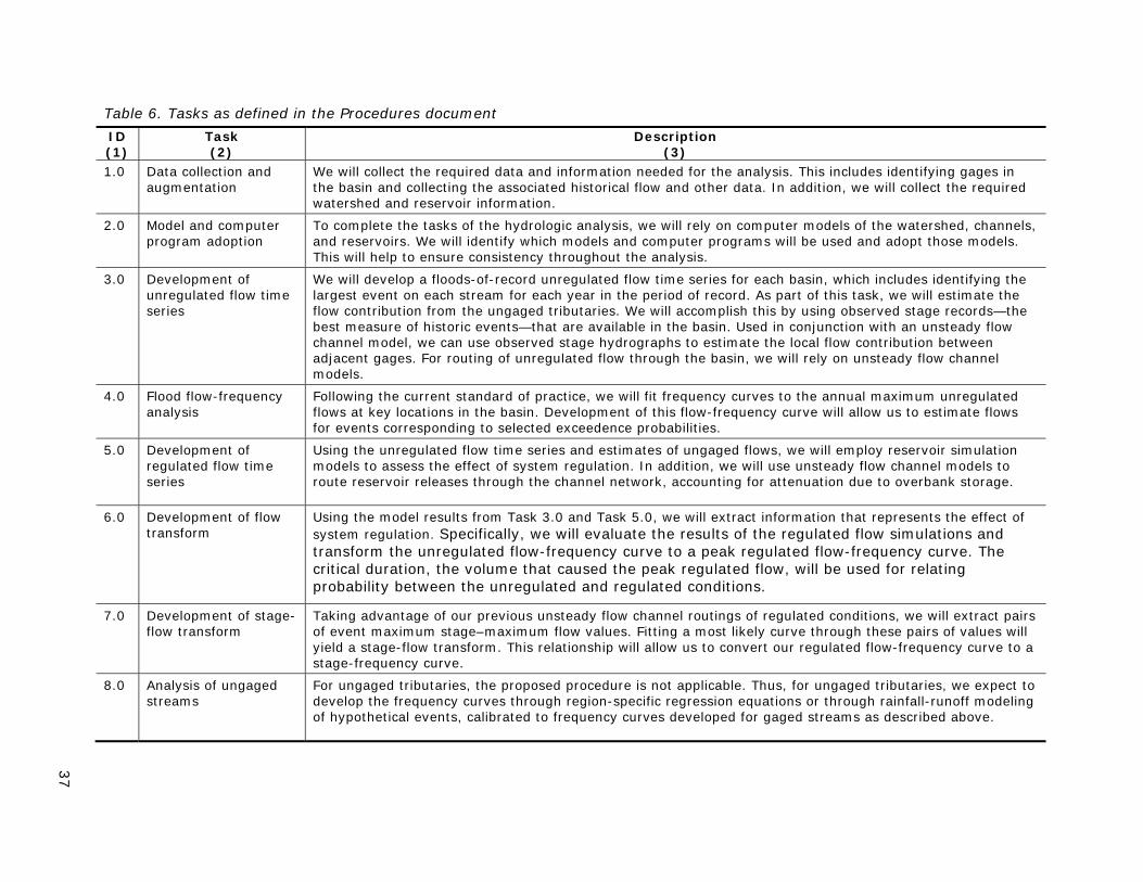
Table 6. Tasks as defined in the Procedures document ID (1)

Task (2)

Description (3)

1.0 Data collection and augmentation

We will collect the required data and information needed for the analysis. This includes identifying gages in the basin and collecting the associated historical flow and other data. In addition, we will collect the required watershed and reservoir information.

2.0 Model and computer program adoption

To complete the tasks of the hydrologic analysis, we will rely on computer models of the watershed, channels, and reservoirs. We will identify which models and computer programs will be used and adopt those models. This will help to ensure consistency throughout the analysis.

3.0 Development of unregulated flow time series

We will develop a floods-of-record unregulated flow time series for each basin, which includes identifying the largest event on each stream for each year in the period of record. As part of this task, we will estimate the flow contribution from the ungaged tributaries. We will accomplish this by using observed stage records—the best measure of historic events—that are available in the basin. Used in conjunction with an unsteady flow channel model, we can use observed stage hydrographs to estimate the local flow contribution between adjacent gages. For routing of unregulated flow through the basin, we will rely on unsteady flow channel models.

4.0 Flood flow-frequency analysis

Following the current standard of practice, we will fit frequency curves to the annual maximum unregulated flows at key locations in the basin. Development of this flow-frequency curve will allow us to estimate flows for events corresponding to selected exceedence probabilities.

5.0 Development of regulated flow time series

Using the unregulated flow time series and estimates of ungaged flows, we will employ reservoir simulation models to assess the effect of system regulation. In addition, we will use unsteady flow channel models to route reservoir releases through the channel network, accounting for attenuation due to overbank storage.

6.0 Development of flow transform

Using the model results from Task 3.0 and Task 5.0, we will extract information that represents the effect of system regulation. Specifically, we will evaluate the results of the regulated flow simulations and transform the unregulated flow-frequency curve to a peak regulated flow-frequency curve. The critical duration, the volume that caused the peak regulated flow, will be used for relating probability between the unregulated and regulated conditions.

7.0 Development of stage-flow transform

Taking advantage of our previous unsteady flow channel routings of regulated conditions, we will extract pairs of event maximum stage–maximum flow values. Fitting a most likely curve through these pairs of values will yield a stage-flow transform. This relationship will allow us to convert our regulated flow-frequency curve to a stage-frequency curve.

8.0 Analysis of ungaged streams

For ungaged tributaries, the proposed procedure is not applicable. Thus, for ungaged tributaries, we expect to develop the frequency curves through region-specific regression equations or through rainfall-runoff modeling of hypothetical events, calibrated to frequency curves developed for gaged streams as described above.

38

Development of unregulated flow time series

The unregulated flow time series will be developed to support the frequency analysis. Key aspects include:

1. Developing upstream boundary conditions (development of reservoir inflows).

2. Developing internal boundary conditions (estimation, application, and distribution of local flows and flows for ungaged watersheds).

3. Selecting the time step of unregulated flow series. Base data are daily, but smaller computational intervals may be needed for some locations depending on study needs.

4. Collecting and augmenting data:

The study requires the rainfall event-based annual maximum peak flow and volumes for various durations at each analysis point.

Some missing data will need to be filled in. The methods that will be used to complete this task depend on how the information will be used. This distinction and a description of the methods are discussed further in Appendix III: Flow time series development and documentation.

5. Identifying the years of record and extending the record length, as needed for purposes of developing a common period of unregulated flow time series for system evaluation (not necessarily for frequency analysis), some streams will require development of additional information than only the observed or gaged data. As part of the development process, some effort is required to estimate missing data and to augment or extend the record length using statistical methods. The exact methods used to complete this effort depend on the expected use of the values.

6. Combining these flow components and routing the flows through the system using a model of the unregulated system. (This model is described in a subsequent section entitled “Study models and computer programs.”)

7. Smoothing the unregulated flow time series.

The technical issues arising from these procedures are addressed in Appendix III: Flow time series development and documentation.

The products of this task will be used in: (1) development of the unregulated-regulated flow transforms, Task 6, and (2) development of the stage-flow transform and stage-frequency curve, Task 7. In addition, the local flows developed here will be used in the simulation of reservoir releases and development of the regulated time series, Task 5.

Unregulated flow-frequency analysis

The unregulated flow-frequency analysis, which corresponds to Task 4, will follow the procedures outlined in Bulletin 17B. Key aspects of this analysis are:

1. Characterizing the frequency curve:

For all analysis locations, the unregulated frequency analysis will be based on annual maximum rainfall events only.

39

2. Separating the rainfall and snowmelt based components of mixed event populations. More information about the issues arising from event separation and selection is provided in the next section entitled “Mixed population analysis and integration into the CVHS.”

3. Developing a single unregulated frequency curve.

4. Developing, and using, regional skews for peak flows and the required volumes associated with various durations.

5. Fitting flow-frequency curves at analysis points.

6. Ensuring consistency in volume-duration-frequency curves.

The technical issues pertaining to these key aspects are addressed in Appendix VI: Unregulated flow-frequency analysis.

The products of this task will be used in: (1) development of the unregulated-regulated flow transforms and family of characteristic curves, Task 6, and (2) development of the stage-flow transform and stage-frequency curve, Task 7.

Mixed population analysis and integration into the CVHS Mixed population analysis

A decision is needed regarding how mixed populations of storm types will be addressed and analyzed in the unregulated flow-frequency analysis that will be completed as part of the CVHS. Guidelines for determining flood flow frequency, Bulletin 17B (hereafter referred to as Bulletin 17B) section B-8, entitled “Mixed population,” notes:

Hydrologic factors and relationships operating during general winter rain flood are usually quite different from those operating during spring snowmelt floods or during local summer cloudburst floods. One example of mixed population is in the Sierra Nevada region of California. Frequency studies there have been made separately for rain floods which occur principally during the months of November through March, and for snowmelt floods, which occur during the months of April through July. Peak flows were segregated by cause—those predominately caused by snowmelt floods and those predominately caused by rain. (Interagency advisory committee on water data [IACWD] 1982.)

Based on a review of past studies in the Sacramento and San Joaquin River basins performed by USACE Sacramento District, a strong precedent exists for treating flows as a mixed population of rain or rain-on-snow (referred to herein as rainfall) and snowmelt events. These past studies include the 2002 Sacramento and San Joaquin river basins comprehensive study (commonly referred to as the Comp study), the 2004 American River Rain Flood Flow Frequency Analysis, and five rain flood flow frequency studies (USACE 1998, 1999a, 1999b, 1999c, 1999d).

Further, based on experience of Corps staff, and specifically the District Hydrologist, the flows in the basin should be treated as a mixed population and separated for flow frequency analysis. Based on this experience, an annual maximum rainfall-event frequency curve is considered the better predictor of extreme events, as compared to the annual maximum flow frequency curve with no event separation.

40

Thus, for the CVHS, a mixed population approach to developing unregulated flow-frequency curves will be taken. At all study locations, rainfall-event frequency curves will be developed. At locations at which the set of annual maximum events includes snowmelt events, snowmelt events will be removed from the sample to yield a rainfall-event only event sample for frequency analysis. At locations in which the set of annual maximum events does not include snowmelt events, the sample of annual maximum events will be used for frequency analysis.

As such, the mixed population approach will be applied to develop rainfall-event frequency curves. Separate snowmelt event frequency curves will not be developed. This is because for the frequency range of interest, rain flood events have been found to drive the regulated condition flow-frequency curve, even in areas of significant snowmelt.

Separation of events to create the time series

Given this decision to account for mixed populations in the CVHS flow-frequency analysis, we must separate rainfall and snowmelt events. To complete this, a consistent process is required to separate the events and find the annual maximums for each. As noted above, Bulletin 17B states that the events should be separated by cause.

Bulletin 17B further cautions: “Separation by calendar periods in lieu of separation by events is not considered hydrologically reasonable unless the events in the separated periods are clearly caused by different hydrometeorologic conditions.” For the Comp Study, the populations were separated by visual inspection of the unregulated flow hydrograph for each water year, and inspection of precipitation and snowpack records when needed and records were available. Analyst judgment was used to determine the beginning of the snowmelt season for each year. In most water years, this served as the date of segregation. If in a water year it was judged that the annual maximum flow resulted from a late season rainfall event occurring after the start of snowmelt, then the date of segregation was adjusted so that late season event would be included in the rainfall population.

Here, the rainfall and snowmelt events for the Sacramento and San Joaquin River basin will be separated by cause in a manner consistent with that used for the Comp Study.

Regional skew and its use in CVHS The need for and use of regional skew parameters is described in Appendix VI. Here, we highlight the coordination between the CVHS team and the US Geological Survey (USGS).

At the onset of the CVHS, the study team identified the need to coordinate with the USGS. At the time, the USGS was working on a regional frequency analysis study. Although the scope of the USGS study is not exactly the same as that of CVHS, common components were identified and it was agreed that these common components should be coordinated.

The first common component is the completion of a peak-flow regional skew analysis. The Corps provided data to the USGS that could be used in its study as well as additional funds for the effort to include those data. A series of meetings from May 2008 to March 2009 took place between Corps and USGS

41

staff to ensure that products from the USGS study could be used for the Corps study and that Corps staff understood the details of the analysis.

At the time, the need for further coordination regarding regional skews for various flow durations was identified and both agencies agreed to continue these discussions. At present, the CVHS team is working with the USGS to complete the regional skew analyses for the 1, 3, 7, 15, and 30-day flow durations. These regional skew parameters will be developed using the separated rainfall annual maximum flow series, consistent with the guidance included in EM 1110-2-1415 in the section on mixed populations:

If annual flood peaks have been separated by causative factors, a generalized skew must be derived for each separate series to apply the log-Pearson Type III distribution as recommended by Bulletin 17B. Plate 1 of Bulletin 17B or any other generalized skew map based on the maximum annual event, irrespective of cause, will not be applicable to any of the separated series. Derivation of generalized skew relations for each series can involve much effort.

Regulated system analysis The unregulated frequency analysis is linked with the assessment of the effects of system regulation (reservoirs, levees, diversions) through the unregulated to regulated flow transform. The unregulated to regulated flow transform process requires the unregulated and regulated flow time series developed in Task 3 and Task 5. The technical issues arising from these procedures are described in Appendix VIII and Appendix X.

Development of regulated flow time series

For regulated system analysis, we take selected events from the unregulated flow time series and simulate those in the regulated system. From the historical events, defined by the unregulated flow time series, we are capturing the system’s response to large, varied events. For example, by simulating various historical and scaled historical events, we can assess the impact to various “storm distributions” (spatial variability) and “storm and runoff timing” (temporal variability).

Portions of the unregulated flow time series (i.e., discrete historical events) will be selected for simulation with our reservoir simulation model, using HEC-ResSim, and our regulated condition channel model, using UNET or HEC-RAS. These simulations will be used to develop the regulated flow time series. This time series reflects:

1. In-stream storage due to reservoir regulation. Issues that can affect reservoir simulation include:

How reservoir operation rules are defined (i.e., which version of the water control manual is used).

How initial conditions for reservoir simulation are defined regarding headwater reservoirs (those without dedicated flood control storage.)

How initial conditions for reservoir simulation are defined regarding project reservoirs (those with dedicated flood control storage.).

2. In-stream attenuation and backwater conditions.

42

3. Off-stream storage due to channel capacity limitations, such as levee overtopping and water entering the floodplain. The channel models are configured such that, if appropriate, the flow can reenter the channel from the floodplains.

4. Off-stream storage due to levee failure, if appropriate. Specific levee failure assumptions for the system will be reflected based on the needs of the analysis or alternative. The channel models are configured such that, if appropriate, the flow can reenter the channel from the floodplains.

The products of this task will be used in: (1) development and application of the unregulated-regulated flow transforms, Task 6, and (2) development of the stage-flow transform and stage-frequency curve, Task 7.

Selection and simulation of historical and scaled-historical inflows

We route selected historical inflows (unregulated flow time series) and scaled versions of those through the regulated system models (HEC-ResSim and HEC-RAS). These simulations produce the regulated flow time series. Here, we selected 4 high flow events (referred to as event patterns) as well as scaled versions of those. The scaled events are needed to understand the response of the system to events more rare than represented by the historical record. For Sacramento, the 1956 and 1965 events are scaled from 0.1 to 2.6. The 1986 and 1997 events are scaled from 0.1 to 2.2. For San Joaquin, the 1951, and 1986 events are scaled from 0.1 to 4.0. The 1956, and 1997 events are scaled from 0.1 to 3.0.

Appendix VIII describes the determination of historical event scaling for extrapolating unregulated-regulated flow transforms and the determination of required additional transforms and inputs.

Development and application of unregulated-regulated flow transform

The transformation process relates unregulated event flows of known probability, to regulated peak flows. The underlying assumption is that for a given event temporal distribution (pattern), there is a “critical” duration that is the best indicator of regulated peak flow. Once the critical duration is identified, the probability associated with the unregulated flow of critical duration is assigned to the regulated peak flow.

The regulated peak flows are pattern- and scale-factor-specific. We develop pattern-specific regulated flow-frequency curves and then combine the curves into a single regulated flow-frequency curve based on the likelihood of each pattern occurring.

The method to find the critical duration, referred to as the “volume window method” as well as additional issues and procedural information on the development of the transform are found in Appendix X.

Adopt final transformed regulated flow-frequency curve

Before adopting final transformed regulated flow-frequency curves, we review the curves to check for consistency and make adjustments as necessary. This includes checking whether individual curves and sets of curves make sense and follow expected trends. If not, the critical duration or weighting of historical patterns is adjusted.

43

Ungaged watershed analysis For some study reaches, and thus analysis points, the floods-of-record analysis approach described earlier in this overview document is not applicable because quality historical information or records are not available in those reaches. Thus, a method for flow-frequency analysis for ungaged watersheds is required. Given the nature of the CVHS, an acceptable, consistent approach is needed.

The basic steps for addressing ungaged watersheds include:

1. Identification of ungaged watersheds requiring frequency analysis.

2. Identification of an appropriate method for each watershed.

3. Rainfall-runoff modeling analysis.

4. Adoption of a flow-frequency curve for each analysis point.

5. Integration of ungaged watershed analysis with floods-of-record analysis.

This approach is described in a separate document entitled Central Valley hydrology study (CVHS): Ungaged watershed analysis. Each of the watershed rainfall-runoff modeling studies has its own separate report included in Appendix XI.

44

Figure 5. Analysis procedure workflow

Task 6.0

Unregulated flow

Regu

late

d pe

ak fl

ow

Task 5.0

Time

Regu

late

d flo

w

Task 3.0

Time

Unr

egul

ated

flow

b

a b

Task 1.0

Data collection

Task 2.0

Model acceptance Reservoir simulation Channel routing a

b

Task 3.2

?

Estimate local flows

A

B

b

Task 4.0

Probability

Unr

egul

ated

flow

Task 6.4

Probability

Regu

late

d flo

w

Expected hydrograph

Time

Regu

late

d flo

w

Characteristic curve

Regulated peak flow

Regu

late

d vo

lum

e

Peak flow

Expected 1-day flow

Expected 3-day flow

45

Term “unregulated flow” and its use in CVHS We use the term “unregulated” herein to refer to a specified state of the system, and the associated derived flows that represents the maximum potential flow delivery to the required downstream analysis points. These maximum potential flows allow us to develop a series of annual maximums upon which we can fit statistics for predicting rare events. The resulting frequency curve serves as a statistical baseline for evaluating flow frequency in the system.

This time series may not be appropriate for uses that call for a full natural flow or unimpaired flow series such as for water reliability analyses or environmental studies, as described in the Technical glossary.

Selection of events for different portions of the analysis Here, we describe how historical events are selected for development of the unregulated to regulated flow transform and how they are used. Further, we highlight the role of scaled historical events, and how the events are scaled. The term “event” is used loosely here to define a simulation time window or a portion of the annual time series considered. The term takes on a slightly different meaning between frequency analysis and system analysis as described below.

Figure illustrates the event selection process. We begin with the entire gage record. For purposes of frequency analysis, we require the appropriate annual maximum flows at each analysis point. All these values, for the entire record length, are required for fitting frequency statistics. The selection of events (period of record definition) for flow-frequency analysis is described here and in Appendix V.

46

Figure 6. Event selection process and resulting datasets

For developing of the unregulated to regulated flow transform, we do not have this same stringent requirement in terms of event selection as with the frequency analysis. Here, we need large historical events that represent storm patterns in the basin. (“Event” is used in this context to define a simulation time window that yields 1 point in the unregulated-regulated flow dataset.) Thus, we require only a subset of events needed to appropriately define the transform for the range of unregulated flows from the p=0.10 to p=0.002 events. This may only be a small percentage of the events needed to support the unregulated flow-frequency analysis. However, we know this small subset will not include events large enough to define the unregulated-regulated transform for unregulated flows less frequent than, for example, the p=0.01 event. Thus, these events must also be the most representative of large system events in the study area as they are scaled to define the upper end of the transforms. Once this subset is selected, the unregulated flows for these events are scaled uniformly and simulated to define the upper end of the flow transform curve.

These datasets are further described in Table 77.

47

Table 7. Dataset descriptions ID (1)

Dataset (2)

Description (3)

1 Events for frequency analysis

To support the frequency analysis, the observed (unregulated) series of annual maximum flows from rainfall events, for various durations, is needed for the period of record. Defining specific events prior to developing the unregulated flow time series at each analysis points is complex and may require an iterative process. For simplicity, here, a continuous simulation of the period of record, coupled with a separation date between rainfall and snowmelt events by year, is employed rather than simulation of discrete events.

2 Historical events for transform development

The most frequent event of interest on the regulated flow-frequency curve is the p=0.10 event. Thus, only a subset of dataset 1 is required. This subset is a small percentage of the events from dataset 1, and only those that represent large, system-wide events. The remaining events would define the transform for a probability range that is not required for this study. Across both basins, the events found to meet this criteria include high flow events in 1951, 1956, 1965, 1986, and 1997.

48

Study products and applications Study products

CVHS products include both hydrologic output and accompanying technical documentation. The CVHS products are described in the CVHS products uses document, CVHS procedures document, and CVHS technical procedures document.

For completeness, we include here a list of the study products:

Unregulated flow-frequency curves at key locations in the Central Valley

Unregulated flow times series (serves as basis of the frequency analysis and transform development)

HEC-ResSim models of the Central Valley

Partial regulated flow times series (Unregulated flows routed through the reservoir simulation model, but not the channel routing model)

In addition to the CVHS products above, included in the study effort is development of “go by” products that complete the process described in the CVHS procedures document and the Technical procedures document. Although these “go by” products may be useful for other applications (such as a first look if the regulated frequency curves may change), the intended purpose is to provide guidance on the appropriate use of the CVHS study products.

The “go by” products include:

Completed regulated flow times series (unregulated flows routed through the reservoir simulation model and the channel routing model, given a specific set of routing assumptions)

Unregulated to regulated flow transform as well as developed critical durations

Beyond the actual results of the CVHS, the CVHS procedures can inform hydrologic analyses required for feasibility studies because the CVHS procedures are Corps procedures. In addition, the technical documentation developed can provide valuable guidance to analysts because it describes issues that arose in the course of the CVHS and how those issues were resolved.

First application regulated condition products The definition of the first application, or “go by”, assumptions include:

1. Reservoir operations for headwater reservoirs (non-project reservoirs) are based on a specific set of assumptions as documented in the technical appendices.

2. Reservoir operations for project reservoirs follow operating rules specified in each reservoirs respective water control manual, and only the dedicated flood pool is used for storing water. Given that this study focuses on flood management, the reservoir models are configured with flood management rules only. Water supply operation and minimum flow requirements are not included in the reservoir simulation models.

49

3. Levees along the channel model are allowed to overtop and water can be stored in the floodplain, but the levees do not fail.

4. Flow splits at bifurcations and system weirs are as represented in the channel routing model described herein.

If the needs for a given study match these assumptions, then the products, after a review of the study needs and the assumptions used in development of the products, can be used directly.

CVHS is not producing a “library” of models, procedures, and/or functions that serve as inputs for every feasibility planning study in the Central Valley. CVHS is a study funded by DWR to meet very specific needs and a specific study area. For a given study, it may be found that the models are appropriate, but specific analysis assumptions differ thus additional hydrologic and/or hydraulic analysis is needed to modify the products to match those assumptions.

Application of study products The results of the CVHS include flow- and volume-frequency curves and hydrographs throughout the system for the unregulated condition and 1 selected regulated condition. In addition, the CVHS provides tools for reanalysis of the system with regards to: (1) changes in the regulated conditions, (2) updates in streamflow records, and (3) potential changes in climate and runoff patterns.

In general, the products of the tasks described herein are those required to support various floodplain analysis goals. This includes, but is not limited to, floodplain mapping, permitting, and planning. How the CVHS products are used requires policy decisions and professional judgment in selection of: (1) scenario choice, and (2) regulated condition assumptions.

The Product uses document illustrates how the study products could be used in floodplain analysis. Here, we identify other potential uses of the procedures and/or projects. These potential product uses include:

Alternative analysis. The products and procedures can be used to support flood damage reduction alternative analyses. Example alternatives include the addition of a flood control reservoir, levee setback, flood bypass, or levee raising. The Product uses document includes an example of how this could be done.

Reservoir re-operation analysis. Similar to alternative analysis, various alternative reservoir operating strategies could be assessed. This analysis would result in a new regulated flow time series which would translate into a new unregulated-regulated flow transform.

408 permit applications. The products and procedures from CVHS would be used to support a 408 permit application following methods consistent with those described in (USACE 2009b).

Climate variability and change analysis. The products and procedures from CVHS could be used to support a climate variability analysis, and in fact, they will be used to do so in a later phase of CVHS. The various climate variability scenarios would have an effect on the unregulated flow time series. Different scenarios involving snowmelt or rainfall intensity factors,

50

for example, would alter the timing and magnitude of the unregulated flow time series. This alternative unregulated flow time series would affect both the unregulated flow-frequency curve as well as the unregulated-regulated flow time series. A description of how the unregulated flow time series would be altered will be the subject of forthcoming documents.

Risk and uncertainty analysis. The products and procedures of the CVHS can be used to assess the risk and uncertainty associated with a system. Specifically they facilitate work within a risk analysis framework as described in the Product uses document.

51

Study models and computer programs Required study models

For CVHS, 3 primary system models are required. These models, and their associated computer programs HEC-RAS and HEC-ResSim, are tabulated in Table 8, and include:

1. Model of the unregulated system for channel routing. A channel routing model representing unregulated conditions is needed to take the derived upstream boundary conditions, specifically the unregulated flow time series, and route and combine those with the derived local flows to construct the final unregulated flow time series at each analysis point. This final time series will serve as the basis of the statistical frequency analysis and development of the unregulated-regulated flow transform.

2. Model of the regulated system for reservoir simulation. A reservoir simulation model representing the system reservoirs and their respective operating rules is needed to take the first step in accounting for system regulation. The results of the reservoir simulation model will be used as input to the next model, the system regulated channel routing model, at selected handoff locations.

3. Model of the regulated system for channel routing. A channel routing model representing regulated conditions is needed to complete the regulated flow time series development. This model is used to account for floodplain storage (due to levee overtopping or, if desired, levee failure) and floodwave translation and attenuation. The results of the simulations with this model will serve as the second half of the unregulated-regulated flow transform and for development of the flow to stage transform. Note that this model is also relevant to the unregulated flow time series development as it is used to support development of the local flow time series.

The primary system routing models, specifically the channel routing models, were selected because they represent the best system models readily available at this time. They are being used to complete the first iteration through the overall study procedures to develop unregulated to regulated flow transforms and flow to stage transforms. The CVHS project team understands that under the DWR Central Valley floodplain evaluation and delineation (CVFED) program, new system channel models will be developed for the regulated conditions. Once these are developed, DWR and CVFED contractors can use these models to reroute the regulated flow hydrographs and refine the transforms. During this process, alternative channel routing assumptions, such as system levee performance, may be used, as well. (The assumption for system levee performance is addressed in Appendix VIII: Completed regulated flow time series.)

[CVFED is a DWR program that has been charged with improving the quality and accuracy of flood hazard data and mapping available to local communities. More information is available at: http://www.water.ca.gov/floodsafe/docs/CVFED.pdf.]

52

Additional study models In addition to the models noted above, various other models and their associated computer programs are required for CVHS. In Table 8 we describe other models required and the computer programs used to run the models.

53

Table 8. Study models and computer programs expected to be used

ID (1)

Purpose (2)

Model (3)

Computer program

(4) Notes

(5) 1 Unregulated flow

channel routing Modified version of the regulated flow channel routing model

HEC-RAS Same base model as for #3, the regulated flow channel model. The model will be modified to reflect the conditions described in Appendix II

2 Reservoir simulation routing

A modified version of the Comp Study reservoir model but updated based on updates to the reservoir simulation software: HEC-ResSim.

HEC-ResSim The extents are similar to the Comp Study models but a fresh look at reservoir operating rules was completed rather than a direct translation from HEC-5. The models were reviewed for consistency with Water Control Manuals. Separate models will be used for the Sacramento system and for the San Joaquin system. Given that this study focuses on flood management, the reservoir models will be configured with flood management rules only. Water supply operation and minimum flow requirements will not be included in the reservoir simulation models.

3 Regulated flowchannel routing

Expanded version of the “Common features” model for the Sacramento system and an HEC-RAS converted version of the Comp Study model for the San Joaquin system

HEC-RAS A modified version of the “Common features” model for the Sacramento system and a modified (converted to HEC-RAS) version of the Comp Study UNET model for the San Joaquin system developed by DWR. Since it does not extend past Colusa on the Sacramento River, geometry from the Comp Study UNET model will be incorporated in the HEC-RAS model for the portion of the system upstream of Colusa.

6 Fitting statisticaldistribution through unregulated flow annual maxima

Log Pearson III PeakFQ and/or PeakFQSA

HEC-SSP could also be used to fit distributions using station statistics and regional skew values.

7 Rainfall runoffsimulation

The specific rainfall runoff models that will be used are documented in the Ungaged watershed analysis procedure document.

HEC-HMS For application to the CVHS, these models will have standard requirements such as using HEC-HMS, having geo-referenced subbasin delineations, and additional criteria detailed in the Ungaged watershed analysis procedure document.

54

Unregulated flow time series development We constructed unregulated flow time series at each analysis location in the study area and fitted unregulated volume-frequency curves to these series using procedures that are consistent with Corps guidance.

The locations most upstream at which we developed unregulated flow time series were the project reservoirs. Thus, for unregulated conditions, the reservoir inflows were needed.

For development of the unregulated flow time series downstream of the reservoir, a routing model was required to simulate the translation, attenuation, and combination of the unregulated flow hydrographs through the system. These flow hydrographs included the upstream boundary conditions (derived reservoir inflows) and intermediate area boundary conditions (estimated local flows). The routing yielded unregulated flow time series that served as the basis of: (1) the unregulated frequency analysis and (2) the unregulated-regulated flow transform.

We developed an unregulated flow time series for the 82 analysis locations in the study area by:

Developing daily unregulated reservoir inflow time series.

Developing and distributing local flow time series.

Augmenting missing data periods.

Smoothing flows from daily to hourly.

Completing the unregulated flow time series at each analysis point.

Estimate daily reservoir inflow Situation

The inflows and upstream boundary conditions for unregulated flow time series development are the major surface storage reservoirs. Typically, the inflows are not measured directly, rather they are inferred based on the observed reservoir elevations and releases. Here, we describe the process for inferring the reservoir inflows and thus developing the upstream boundary conditions for the unregulated flow time series.

Pertinent guidance and discussion

No specific guidance addresses the calculations to infer the reservoir inflows. However, EM 1110-2-1420, paragraph 5-4b titled “Unregulated conditions” does note the following:

It is not always feasible to convert flows to natural conditions. Often, required data are not available. Also, the hydrologic effects and timing of some basin developments are not known to sufficiently define the required adjustments. An alternative is to adjust the data to a uniform basin condition, usually near current time. The primary adjustments should remove special influences, such as major reservoirs and diversions that would cause unnatural variations of flow.

However, the governing equation is the continuity equation in which, for a given time step, the average inflow less the outflow equals the change in

55

reservoir storage. By convention in the Central Valley, these calculations are completed on a 1-day time step, thus midnight to midnight values are used. This is consistent with the work completed for the Comp Study (USACE 2002a).

As noted in the Comp Study documentation, significant effort was expended to develop the unregulated flow time series at the project reservoirs. The process to develop these series is documented in Sacramento and San Joaquin river basins comprehensive study, Technical studies documentation, Appendix B: Synthetic hydrology technical documentation (USACE 2002b). However, the time series stopped at the 1997 water year.

In the Comp Study, for some watersheds, non-flood control reservoirs upstream of the project reservoirs were found to store or attenuate runoff enough that the effect was accounted for in the calculation of unregulated flows at project reservoirs. We list in Table 99 and Table these project reservoirs and corresponding headwater reservoirs accounted for in the calculations. For the project reservoirs not listed, no accounting for upstream storage was made. Thus the observed outflows and storages were used solely to infer the reservoir inflows. The lag time used to account for the travel time between each headwater reservoir and the project reservoir is provided in column 3 of the tables.

56

Table 9. Sacramento basin headwater reservoirs accounted for in development of unregulated flows at project reservoirs

ID (1)

Project reservoir (2)

Gross pool

capacity (ac-ft)

(3)

Lag time

(days) (4)

Headwater reservoir

(5) 1 Folsom 977,000 1 French Meadows

1 Hell Hole

1 Ice House

1 Loon Lake

1 Union Valley

1 Ice House

2 Oroville 3,538,000 1 Little Grass Valley 0 Sly Creek 1 Frenchman 1 Davis 1 Mountain Meadows 1 Almanor 1 Antelope 1 Butt Valley 1 Bucks

3 Shasta 4,552,000 0 Britton (Pit 3) 0 Pit 6 0 Pit 7 0 McCloud

4 Black Butte 136,193 0 East Park 0 Stony Gorge

57

Table 10. San Joaquin basin headwater reservoirs accounted for in development of unregulated flows at project reservoirs

ID (1)

Project reservoir (2)

Gross pool

capacity (ac-ft)

(3)

Lag time

(days) (4)

Headwater reservoir

(5) 1 Pine Flat 1,001,055 0 Courtright/Wishon

2 Camanche 430,900 0 Lower Bear 0 Salt Springs 0 Pardee

3 Friant 520,500 0 Thomas A. Edison 0 Florence 0 Huntington 0 Shaver 0 Redinger 0 Mammoth 0 Bass

4 New Melones 2,420,000 0 Beardsley 0 Donnells 0 New Spicer Meadows

5 Don Pedro 2,030,000 0 Hetch Hetchy 0 Cherry Valley 0 Eleanor

Study procedure

Consistent with the Comp Study, we developed the daily unregulated reservoir inflow time series for project reservoirs using the continuity equation, in which, for a given time step, the average inflow equals the outflow plus the change in reservoir storage. For the calculation of these inflows, the source of the observed reservoir outflows and observed changes in storage was the Corps’ database. By convention in the Central Valley, these calculations were completed on a 1-day time step, thus midnight to midnight values were used.

Estimation of ungaged local flows Situation

In the context of this task, the ungaged watersheds are the local runoff along major streams. Thus, we also refer to these as local flows or internal boundary conditions (hydraulic modeling term) for the unregulated flow time series development. Because stream gages measure total flow in the channel, the flows from these incremental watershed portions are not gaged directly. Thus, the flow contribution for historical events must be inferred from observed data.

58

Key aspects regarding inferring the local flow contribution within the context of the CVHS are:

An underlying assumption is that the local flow is small relative to the total flow at the given point.

The flow time series for the incremental watershed area, by itself, is not applicable as the basis of a flow frequency analysis.

Where a flow frequency analysis is needed on a stream that is included in the incremental area, a different method than those described in this section would be required. For example, these scenarios are addressed in Procedure document Task 8.


Guidance on estimating local flow contribution is offered in EM 1110-2-1420 when discussing missing data. Section 5-4f, paragraph (2) notes:

Flow estimates for ungaged locations can be estimated satisfactorily on a flow per basin area basis in some cases, particularly where a gauge exists on the same stream. In most cases, however, it is necessary to correlate mean flow logarithms (and sometimes standard deviation of flow logarithms) with logarithms of drainage area size, logarithm of normal seasonal precipitation, and other basin characteristics. Correlation procedures and suggested basin characteristics are described in Chapter 9 of EM 1110-2-1415.

Estimation of local flows can be an involved process. The preferred method is to estimate the local flow contribution directly for historical events from observed flow or stage data. To do this, the observed data at the upstream point is routed downstream with a channel model to the next observation point. There, the inferred flow is the difference in routed flow and the observed flow. However, the ability to estimate the flow time series depends on the availability of stream gage data, the quality of that data, and the channel models.

When stream gage data are not available, another option is to use historical precipitation data and a rainfall-runoff model to develop a flow time series. This requires development of a rainfall-runoff model for the local area and sufficient precipitation data in terms of temporal and spatial distribution. The rainfall-runoff model would then be used in a “continuous simulation” fashion to develop an unregulated flow time series. The resulting flows would be sensitive to estimates of loss methods and parameters and the accuracy of the flow transform. Thus, the results would be expected to have greater uncertainty than the preferred method.

For many cases, neither streamflow data nor rainfall data are available. Thus, the third option is to rely on analysis of nearby gaged watersheds through regression analysis. For example, the flow from a local area may be estimated as a percent of the flow from a nearby gaged watershed based on a comparison of watershed areas.

Even with the first option—observed flows and a channel model—several challenges still exist for estimating the local flows. The primary challenges are the limitations of the channel model and the use of historical data. Specifically, these challenges include:

59

Use of a model of the unregulated system and levees with historical data. Thus caution must be exercised when using, for example, stage data from 1986 with a channel model based on 2009 geometry.

Use of historical data that may contain levee breaks or other “event specific” factors. Again, caution must be exercised when using the data.

The actual local flow contribution may simply be less than the resolution of flow data available from the gage data, making difficult the estimation of small local flows.

In general, the properties of each local flow area will be examined to determine the appropriate method. In addition, the results of the analysis will also be examined to ensure that the results are within a reasonable and acceptable range.

Study procedure

For the CVHS, we will:

Identify the “local flow” subareas that require a flow estimation analysis by delineating watersheds at the stream gage locations.

Assess each subarea with regards to watershed properties and availability of historical data.

Select the appropriate analysis approach for each subarea. Preference between the methods will be given in the order described above.

Details of the local flow estimation may be found in Appendix III.

Application and distribution of local flow Situation

Once the local flows for a given area have been estimated, they are input to the unregulated-condition channel model for completion of the unregulated flow time series. In subsequent steps, this same local flow is input to the regulated condition channel model in a consistent manner. In application of that local flow, we must consider factors such as location and timing. For example, should all the estimated local flow be applied at one cross section? And, if the application location is different than the downstream gage, does the timing of the flow need to be adjusted to account for the travel time between that cross section and the downstream gage?


While the EMs, such as EM 1110-2-1417 Section 18-3e and Section 19-1c as noted in Table , address local flows in general, guidance on application of such flows is not specifically provided. Thus this is an issue of system representation, rather than an issue of methodology.

60

Three (3) basic options for distributing the local flow in the channel model are available:

Option 1: Distribute as a point lateral inflow. With this option, the local flow, for the sub areas, would be applied at a specific point or cross section. If the selected point is other than the downstream gage location, then the flow may need to be lagged (backwards) an amount approximately equal to the travel time of that point to the downstream gage.

Option 2: Distribute as a uniformly-distributed lateral inflow. With this option, the local flow would be distributed uniformly from the upstream gage to the downstream gage.

Option 3: Distribute as a combination of the 2 options noted. With this option, a combination of the other 2 options would be used based on an analysis of the characteristics of that subarea. For example, 50% of the local flow may be attributed to a defined small tributary stream and the remaining 50% is uniformly-distributed throughout the reach. An analysis of incremental contributing area by cross section (such as would be available with a flow accumulation grid) could be used to define the balance.

Study procedure

For the CVHS, option 3 from the list above will be used. The local flow will be distributed as a combination of point lateral inflows and uniformly-distributed lateral inflows. The balance given to the 2 options will be based on the change in the cumulative watershed area per cross section. We will use the flow accumulation grid developed for the study using GIS tools for this analysis. As deemed significant, based on a review of each subarea, point lateral inflows will be lagged based on the average travel time in the channel. Details of the local flow distributing may be found in Appendix III.

Approach for extending data or filling in gaps Situation

A challenge of any watershed study is the availability of gage data, both in terms of spatial distribution and in terms of length of record. For a study the magnitude of the CVHS, an additional challenge becomes the availability of a long, common record period to support analysis in the main stem reaches and for simulating large events for development of flow transforms. Thus, in construction of the unregulated flow time series, it may be necessary to “fill

Table 11. Pertinent guidance for distribution of local flow

Reference (1)

Guidance (2)

EM 1417 Section 18-5e

A levee or floodwall blocks the natural drainage of local runoff into the channel.

EM 1417 Section 19-1c

Local flows are then added at the downstream location to obtain the total flow hydrograph. This type of approach is adequate as long as there are no significant backwater effects or discontinuities in the water surface because of jumps or bores.

61

in” gaps for missing data or to extend record lengths for specific tributaries or streams.


Table 12 lists the pertinent guidance for augmenting and extending gage data found in EM 1110-2-1415.

Table 12. Pertinent guidance for extending data or filling in gaps

Reference (1)

Quote from reference / guidance (2)

EM 1110-2-1420, paragraph 5-5f: Extending and filling in historic records

Statistical techniques can be used to augment existing historic records by either “filling in” missing flow values or extending the observed record at a gauge based on observations at other gauges.

EM 1110-2-1420, paragraph 6-6f: Runoff record interruptions

In cases where no runoff records are available on the stream concerned, it is possible to estimate the frequency curve as a whole using regional generalizations. An alternative method is to estimate a complete series of individual floods from recorded precipitation by continuous hydrologic simulation and perform conventional frequency analysis on the simulated record.

EM 1110-2-1415, paragraph 2-3d: Estimating missing events

Where a longer or more complete record at a nearby station exists, it can be used to extend the effective length of record at a location by adjusting frequency statistics (Section 3-7) or estimating missing events through correlation (Chapter 12).

In the context of the CVHS, the unregulated time series will be used for analysis in 2 category groups: (1) the unregulated flow-frequency analysis and (2) assessing the effects of regulation. The specific methods used to complete this data augmentation and extension effort depend on the expected use of the values, i.e. what group the “filled in” data will be used for. Specifically, the methods appropriate for reconstruction of historical events for system simulation may not be appropriate for developing data to support frequency analysis. For either case, 1 option is to do nothing: not fill in the gap or extend the record and simply not use flows from that year or from that stream in the analysis. However, by augmenting the data, we can take advantage of all information available.

Description of methods to support flow-frequency analysis

Regression techniques are commonly used where the intended purpose is for reconstruction of a historical event (event time series of flow or hydrograph). However such techniques are not appropriate for frequency curve development as they do not preserve the “true” properties of the fitted distribution. As noted in EM 1110-2-1415, “the use of regression analysis produces estimates with a smaller variance than that exhibited by the recorded data.” Thus an alternative method, such as maintenance of variance extension (MOVE1), should be used where data are filled in for the purposes of frequency analysis. MOVE1 techniques are most commonly used when developing a series of annual maximum values for a specified duration, not re-creation of historical event hydrographs.

62

MOVE1 uses the correlation between nearby stream gages to extend record lengths. This procedure is described and evaluated in “A Comparison of Four Streamflow Record Extension Techniques” (Hirsch 1982), and “A generalized maintenance of variance extension procedure for extending correlated series” (Gygier et al 1989).

Methods to support assessing the effects of regulation

Linear regression analyses likely give the best estimate of flows (or a time series of flow) for a single historical event. Thus, when filling in missing data from a flow time series for the purposes of simulating an event to pair unregulated and regulated flow values, this method can be used. However, when the time series will be used for frequency analysis, linear regression may not be appropriate as noted above.

For the Comp Study, linear regression analysis was used to “fill in” event hydrographs for various streams. Commonly, the flow from one tributary was estimated as a function of a nearby gaged tributary.

Study procedure

For the CVHS, augmentation of data may be needed for both frequency analysis and assessment of regulation effects. MOVE1 techniques will be used for determining the missing values for a series of annual maximums. Linear regression will be used for reconstruction of historical events for system simulation. In general, for the CVHS, the need to fill in missing data to support frequency analysis will be limited. Rather, especially for the tributaries, the period of record for the reach will reflect those years where observed data are available for the majority of the contributing watershed. Thus, for each analysis point, a different historical record length could be used. This is consistent with the frequency curves developed in the Comp Study. For the CVHS, the period of record for study reaches not included in the Comp Study will be determined based on the period of record for which the majority of the contributing area is gaged. Details on data augmentation can be found in Appendix III.

Smooth unregulated flow time series

Situation

The time step of the unregulated flow time series inferred from reservoir outflows and change in storage is 1 day. This time step is appropriate for frequency analysis in a regulated system such as the Central Valley. However, when evaluating the effects of the regulated system, a smaller time step, and thus a “more defined” inflow hydrograph, may be desired. A refined unregulated flow time series may be needed to better represent the reservoir outflow hydrographs.


Recall that the unregulated time series is used both in frequency analysis and evaluation of system regulation effects.

For the purposes of unregulated frequency analysis, an unregulated times series with a temporal resolution of 1 day is acceptable for regulated systems such as those in the Sacramento and San Joaquin river basins. Specifically,

63

the unregulated time series will be used to develop a comprehensive set of flow-frequency curves.

However, when simulating the effects of the reservoir system, some reservoir releases are sensitive to hourly inflows and storages. (The time step of the HEC-ResSim model will be 1 hour.) Thus, a more refined inflow hydrograph may result in a different outflow hydrograph, as compared to using a daily average inflow. This is a result of ungated weirs and operations based on emergency spillway release diagrams, for example. For the Comp Study, a single selected historical event (the 1997 event for the Sacramento River basin, and the 1955 event for the San Joaquin River basin) was used to develop hourly inflow time series. However, all historical events are not patterned with this shape, thus use of this single hydrograph shape may bias the results.

Study procedure

The daily unregulated flow time series are appropriate for frequency analysis. However daily upstream and intermediate boundary conditions do not have the temporal resolution required by the CVHS procedures for assessing the effects of regulation, particularly releases as indicated on the emergency spillway release diagram (ESRD). Therefore, the daily reservoir inflows and daily estimated local flows were “smoothed” to hourly time series. This smoothing was completed using a mass balance algorithm that interpolates the shape of the hydrograph and estimates peak hourly flows while maintaining daily volumes consistent with the original time series. These smoothed series were used for both unregulated and regulated flow simulations. Details on data smoothing can be found in Appendix III.

Procedures for routing unregulated flows through the system

Situation

For development of the unregulated flow time series at each analysis point, a routing model is required to simulate the translation, attenuation, and combination of the unregulated flow hydrographs through the system. These flow hydrographs include the upstream boundary conditions (derived reservoir inflows) and intermediate boundary conditions (estimated local flows). The routing of these hydrographs must be such that the resulting unregulated flow time series is sufficient to serve as the basis of: (1) the unregulated flow frequency analysis and (2) the unregulated-regulated flow transform.


Selected guidance for routing unregulated flows is noted in Table 4.

64

Table 4. Pertinent guidance for routing unregulated flows

Reference (1)

Guidance (2)

Bulletin 17B frequently asked questions (http://acwi.gov/hydrology/Frequency/B17bFAQ.html#data)

…factors such as flow regulation by dams, dam failures, stormwater management, effects of development (or reversion to undeveloped conditions) in the flood plain, stream channel improvement or restoration, and the effects of mining, forestry, agriculture, or reclamation from those activities, all have the potential to make all or part of the record unrepresentative of future flood risk. The significance of these factors and the nature of any adjustments that might be applied for estimation of future flood risk cannot be predicted in general and depends on the specific situation at each site; no simple guidelines can be given that could safely be followed blindly or dogmatically.

EM 1110-2-1417, paragraph 9-4d(2)

To analyze the transition from main channel to overbank flows, the modeling technique must account for varying conveyance between the main channel and the overbank areas. For 1-D flow models, this is normally accomplished by calculating the hydraulic properties of the main channel and the overbank areas separately, then combining them to formulate a composite set of hydraulic relationships.

Consistent with standards defined in the Bulletin 17B (IACWD 1982), the flow time series should be free of regulation and channel improvements if it is to be used as the basis of frequency analysis. Thus, the routing, to the extent practical, should be free of the effects of flood control systems including dams, weirs, levees, and diversions. In addition, for the CVHS, this routing model should be such that it can be paired with the later regulated-condition routing model to extract unregulated to regulated data points. Within the context of the CVHS, the regulating features of the system can be separated into 2 groups: (1) reservoirs and (2) levees.

The removal of the effects of regulation due to reservoirs is a relatively straightforward task. This removal is completed for the CVHS by developing unregulated reservoir inflows, and is detailed above in the section entitled “Development of reservoir inflows.” However, the removal of regulation effects due to the levee system is more challenging because of the floodplain storage and flow splits of the system.

The effects of floodplain storage can be removed from the unregulated channel model by confining flows to the channel for development of the unregulated time series. While the floodplain storage in Sacramento and San Joaquin river flood control system can effectively be removed from the channel model, the flow splits (i.e. the flood bypasses) cannot similarly be “physically” removed from the unregulated channel model. However, the effects of the flow splits can be limited by combining flows in the mainstem and bypasses for frequency analysis. Thus, a composite unregulated flow time series, for the purposed of frequency analysis, can be developed by adding the flow hydrograph in the Yolo Bypass with a complimentary flow hydrograph in the Sacramento River, for example. This “at latitude” approach, consistent with frequency analysis in the Comp Study, allows us to develop annual maximum flow values that represent the total contribution of flow from the upstream watershed.

65

In these cases, the unregulated-regulated flow transform would be developed such that the regulated peak flow is specific to a given analysis point. For example, a relationship might be the composite unregulated flow at latitude Sacramento to the regulated flow in the Yolo Bypass at a specific cross section.

For the Comp Study, hydrologic routing algorithms, specifically Muskingum routing, was used to route unregulated flows through the system. Challenges with this approach include:

A consistent set of parameters, across a wide range of flow values, is used. For actual events, travel time varies with the flow magnitude. In addition, limited data are available to calibrate the hydrologic routing parameters used for the range of flows that will be simulated.

Limited refinement in the definition of the routing reaches is available. Unregulated flows are only known at the upstream and downstream ends of the routing reaches.

Analysis points must be collocated across all analyses for development of the various CVHS products.

Use of a channel model (unsteady flow hydraulics model) helps to overcome these challenges. Additional advantages include:

An increased spatial resolution of the channel.

A refinement to the translation and attenuation of the system.

An inclusion of the effects of in-channel storage.

Study procedure

We developed an unregulated channel model for the CVHS by taking the selected regulated channel model, and removing the effects of floodplain storage. For the CVHS, we modeled the unregulated conditions by confining flow within the channel created by the current levee alignment. While confining flows to a leveed channel does not truly represent a watershed’s unregulated condition, this confinement does allow for development of the maximum potential flow series needed for the analysis.

We combined the flows for the channel mainstems and bypasses in a manner consistent with the Comp Study. Table 14 shows an example of how these time series were added together.

Table 5. Example relationship of analysis point to channel model cross section(s)

ID (1)

Analysis point (2)

Computation of unregulated flow (3)

1 SAC40 SAC XS 72 + SUT XS 60

66

Unregulated frequency analysis Commonly accepted procedures to develop unregulated flow-frequency curves are specified in Bulletin 17B (IACWD 1982). The current standard-of-practice is to fit a Pearson III (LPIII) distribution to the logarithmic transforms of annual maximum series identified from streamgage data. Additional guidance for fitting frequency curves to volumes for a given duration is provided by EM 1110-2-1415 (USACE 1993).

For this analysis, we used the unregulated flows to develop such an annual maximum series. The annual maximum series represents the annual maximum rainfall and/or rain-on-snow event. As described in Appendix IV and V, a separation date was identified for key locations in the basin for each year as to the transition from rain-on-snow events to snowmelt-driven events. Based on that separation date, the maximum volumes were extracted.

We developed unregulated frequency curves following general guidelines specified in Bulletin 17B (IACWD 1982), EM 1110-2-1415 (USACE 1993), and the current standards of practice. Annual maximums are transformed into logarithmic data and a LPIII distribution is fit to the data. However, the final approach that was adopted differed between the Sacramento River and the San Joaquin River basins.

San Joaquin River Basin: For the San Joaquin River Basin, we applied Bulletin 17B procedures including fitting an LPIII distribution to annual maximums, and weighting individual station skew with regional skew values. This approach worked well in the San Joaquin River Basin. USACE partnered with USGS to produce a new regional skew study for volume-duration (Regional Skews for Selected Flood Durations for the Central Valley Region, California, Based on Data Through Water Year 2008, USGS Scientific Investigations Report 2012-2150). The report covers regional skew for 1-, 3-,7-, 15-, and 30-day volume durations. The resulting skew coefficients are based on mean watershed elevation as shown in the Figure 7 below. For each analysis location, we:

Performed separation of seasonal data (rainflood versus snowmelt).

Identified the annual maximum series.

Calculated regional skew values for each duration of interest using relationships developed by the USGS.

Fitted LPIII distributions to the annual maximum series following Bulletin 17B procedures and USGS’s flow-frequency software PeakFQ v5.2

Reviewed, adjusted if needed, and adopted the curves, checking them for consistency and comparing them to previously accepted values.

67

Figure 7: Excerpt from Regional Skews for Selected Flood Durations for the Central Valley Region, California, Based on Data Through Water Year 2008, USGS Scientific Investigations Report 2012-2150

Sacramento River Basin: Unlike the San Joaquin River Basin, using PeakFQ software and weighting station skew with the 2012 USGS regional skew study values for volume-duration did not result in a good fit to sampled data at many flow frequency locations within the Sacramento River Basin. There are several factors at work that explain this result. First, the San Joaquin River Basin has higher mountain ranges and elevation bands, with deeper snow and more snowpack covered area. Despite attempts to separate snowmelt and rainflood events, snowmelt acts like baseflow on the San Joaquin River and its tributaries. It is difficult to entirely remove it from the flow record. The snowmelt component serves to lift the lower tails of the sampled data. These lower tails are water years with less rainfall including drought years. The snowmelt component naturally raises the flow, resulting in fewer identified low outliers. In comparison, the Sacramento River is more prone to having low outliers. Drought years can be quite dry in the Central Valley and the soils may readily absorb a significant amount of the precipitation that does fall. On the other hand, large storms driven by atmospheric rivers can contain enormous amounts of precipitation such that the most intense part of the storm falls on saturated ground. California precipitation is known to have some of the largest variability (highest standard deviation) of all states in the country. The runoff response during drier years can be essentially considered non-homogenous with the runoff response during wetter years when the soils are more saturated. A third factor is related to mean basin elevation and application of the 2012 USGS regional skew values. Many Sacramento River tributaries have a significant portion of their watershed area that falls between elevation bands 3,000 to 4,000 feet above sea level. In the chart above, notice that the regional skew values change dramatically between 3,000 to 4,000 feet mean basin elevation. In this range, the regional skew

68

values change significantly in relation to only a few hundred feet change in elevation. It was found that weighting of the station skew with regional skew at many locations in the upper Sacramento River (below Shasta Dam) resulted in a poorer fit of the frequency curve to the period of record data, as opposed to using station skew only. As the focus of CVHS is upon rare floods, the fit of the upper end of the frequency curve was of concern. After attempting to use the same methodology as was applied to the San Joaquin River Basin upon the Sacramento River Basin, it was decided that other curve fitting methods would be tested to determine if improvements could be obtained in this part of the Central Valley.

EMA/MGB/WGT was applied to the Sacramento basin locations using Dr. Tim Cohn’s software tool PeakfqSA v0.972. Where the GB test had identified only a few (0 to 3) outliers at most locations, the MGB test sometimes identified 20 to 50. This was much higher than the number of outliers identified in the regional volume skew study (SIR 2012-5130). Because skew and standard of deviation are coupled, we concluded regional skew from the volume skew study was not appropriate for this application in the Sacramento basin. This was validated by attempts to apply regional skew in many locations in this basin. Station skew was adopted instead. In reviewing the resulting curves, EMA/MGB/STA yielded regionally much improved comparisons between the analytical curves and the largest plotted flows.

As noted in the section on Procedures, for some analysis points, the flow-frequency curve was developed through rainfall-runoff simulations. The processes to develop these curves for each watershed are described in Appendix XI.

Separation of seasonal data Situation

The annual maximum rainfall (here, referring to both rain and rain on snow) and snowmelt events are separated for the CVHS unregulated flow-frequency analysis. Rainflood frequency curves have been developed at all study analysis locations in the Sacramento River and San Joaquin basins.


The guidance for separation of mixed populations resulting from seasonal data seasonal data is Guidelines for determining flood flow-frequency, Bulletin 17B (hereafter referred to as Bulletin 17B) and EM1110-2-1415. Specifically, Bulletin 17B section B-8, entitled “Mixed population,” notes:

Hydrologic factors and relationships operating during general winter rain flood are usually quite different from those operating during spring snowmelt floods or during local summer cloudburst floods. One example of mixed population is in the Sierra Nevada region of California. Frequency studies there have been made separately for rain floods which occur principally during the months of November through March, and for snowmelt floods, which occur during the months of April through July. Peak flows were segregated by cause—those predominately caused by snowmelt floods and those predominately caused by rain. (Interagency advisory committee on water data [IACWD] 1982.)

69

For the Comp Study, the populations were separated by visual inspection of the unregulated flow hydrograph, and as necessary, inspection of the precipitation, temperature, and snowpack data for each water year. Analyst judgment was used to determine the beginning of the snowmelt season for each year. In most water years, this served as the date of segregation. If in a water year it was judged that the annual maximum flow was the result of a late season rainfall event occurring after the start of snowmelt, then the date of segregation was adjusted so that late season event would be included in the rainfall population.

Study procedure

For the CVHS, we rely on the data that represented rain or rain-on-snow events. The procedure steps and final separation dates for identifying rainflood versus spring snowmelt events are detailed in Appendix V. This document formalizes and describes the process for event separation, which are consistent with the steps from the Comp Study.

Identify annual maximum series

Situation

For analysis of regulated systems, such as the Sacramento and San Joaquin river basins, flood volumes are important in developing regulated peak flow-frequency curves. Thus, a comprehensive series of unregulated volume-duration-frequency curves at each analysis point is needed.


The pertinent guidance and discussions in the EMs with regards to durations used to define the comprehensive series of curves is listed in Table 6.

Table 6. Pertinent guidance for the specification of volume-durations

Reference (1)

Guidance (2)

EM 1110-2-1415, paragraph 3-8a

Flood volume-duration data normally obtained from the USGS WATSTORE files consists of data for 1, 3, 5, 7, 15, 30, 60, 90, 120, and 183 days.

Runoff volumes are expressed as average flows in order that peak flows and volumes can be readily compared and coordinated. Whenever it is necessary to consider flows separately for a portion of the water year such as the rain season or snowmelt season, the same durations (up to the 30-day or 90-day values) are selected from flows during that season only.

EM 1110-2-1420, paragraph 3-8b

Data to be used for a comprehensive flood volume-duration frequency study should be selected from nearly complete water year records. Unless overriding reasons exist, the 1-, 3-, 5-, 7-, 15-, 30-, 60-, 90-, 120-, and 183-day durations should be used.

As noted, the guidance calls for durations as long as 183 days. However, in the Sacramento and San Joaquin river basins, these longer durations are not required. Typically, rain-flood events in the Central Valley and Sierra Nevada

70

regions do not last longer than 10-15 days. For this reason not all the standard durations are needed for the CVHS.

For the Comp Study, peak (in some cases), 1-day, 3-day, 7-day, 15-day, and 30-day curves were developed.

Study procedure We identified the annual maximum series by extracting, from the unregulated flow time series, the volumes associated with the 1-, 3-, 7-, 15-, and 30-day durations, consistent with the Comp Study. This information is detailed in Appendix V.

Calculate regional skew values Situation

Bulletin 17B calls for the use of a regional skew value in adopting the log-Pearson Type III distribution parameters. The adopted skew value used to derive the final unregulated flow-frequency curve is thus a function of the station skew value and the regional skew value. Although use of the regional skew is called for in Bulletin 17B, regional skews for all the required flow durations are not available in the Sacramento and San Joaquin river basins.


The use and development of regional skew values are documented in Bulletin 17B and EM 1110-2-1415. In fact, EM 1110-2-1415 stipulates that Bulletin 17B should be used as guidance for development of regional skews and frequency functions.

Bulletin 17B recommends that the method of choice used to develop a regional skew value should be selected based on the lowest mean square error of 1 of 3 methods:

Method 1: Region area-average skew.

Method 2: Skew isoline map.

Method 3: Predictive equations.

There is some flexibility in Bulletin 17B to allow for the use of new or improved methods.

Study procedure

For this analysis, we calculated regional skew values for the peak flows and 1-, 3-, 7-, 15-, and 30-day volumes using the relationships developed by the USGS (USGS 2010). These relationships are published in:

USGS regional skew study for peak flows (SIR 2010-5260).

USGS regional skew study for 1-day, 3-day, 7-day, 15-day, 30-day flow durations (SIR 2012-5130).

Both of these studies were completed with Corps support as part of the CVHS.

The manner in which these regional skew values were used depended on the basin. For example, the values were explicitly used in the San Joaquin basin in the adopted curves. However, in the Sacramento basin, they were used during the fitting process, but ultimately not used explicitly. More details on

71

this follow in the later sections of this report. The values calculated for each analysis location and duration of interest are shown in Appendix VI.

Fit frequency curves Situation

Once the annual maximum series of unregulated flows are developed and extracted, the next step is to fit a statistical distribution through the data. This statistical distribution is then used to predict flows for rare events.


The standard of practice, outlined in Bulletin 17B, is to fit flow-frequency curves using a log-Pearson Type III distribution with an adopted skew coefficient (developed by weighting the regional and station skews using the skews’ associated error).

Key excerpts from Bulletin 17B and EM 1110-2-1415 are listed in Table 7.

Table 7. Pertinent guidance for fitting flow-frequency curves

Reference (1)

Guidance (2)

Bulletin 17B, section V.B

The Pearson Type III distribution with log transformation of the data (log-Pearson Type III distribution) should be the base method for analysis of annual series data using a generalized skew coefficient.

EM 1110-2-1415, paragraph 3-2a

The analytical frequency procedure recommended for annual maximum streamflows is the logarithmic Pearson type III distribution.

Bulletin 17B, section V.B.4

The station skew and generalized skew coefficient can be combined to form a better estimate of the skew for a given watershed. Under the assumption that the generalized skew is unbiased and independent of the station skew, the mean-square error (MSE) of the weighted estimate is minimized by weighting the station and generalized skew in inverse proportion to their individual mean-square errors.

Study procedure

To fit frequency curves to the annual maximum series we used: (1) the statistics of the logarithmic transforms of unregulated flow time series (mean, standard deviation, and skew), and (2) the regional skew values for the peak flow, and 1-, 3-, 7-, 15-, and 30-day calculated using relationships developed by the USGS (2010).

For fitting of the distributions, 2 algorithms were considered:

1. Method of Moments (MOM) with Grubbs-Beck (GB) outlier test. For implementation of this algorithm, USGS software tool Peakfq v5.2 was used.

2. Expected Moments Algorithm (EMA) with Multiple Grubbs-Beck (MGB) outlier test. For implementation of this algorithm, Dr. Tim Cohn’s software tool PeakfqSA v0.972 was used.

72

During the fitting process, various tests were completed to identify by basin which method and inputs achieved the best fit both at site and regionally to the dataset. The final selected methods and algorithms used for the Sacramento basin was EMA with MGB and using the station skew (EMA/MGB/STA). For the San Joaquin basin, MOM with GB and used a weighted skew (MOM/GB/WGT) was selected. The weighted skew is a function of both the at-site skew and the regional skew. A description of the process that led to adoption of these approaches is provided in Appendix VI. As described in that sections are instances where slight modifications to the general basin approach was merited.

Review and adopt curves Situation

The series of annual maximums at each analysis point, used for fitting the unregulated flow-frequency curves are based on consistent historical events. Thus, it would be expected that the resulting frequency curves would also be consistent. For example, unless specific circumstances dictate otherwise, the p=0.01 flow would increase as you move downstream. However, a chance exists that inconsistencies may show up. Thus, a careful review of the frequency analysis results is required.


No specific guidance exists regarding the consistency in the volume-duration-frequency curves described above. However guidance does exist regarding the development of hypothetical events that should be consistent with the volume-duration-frequency curves, as listed in Table 8. In addition the Comp Study examined the developed frequency curves for consistency and reasonableness. This method is also listed in Table 8. As seen, expert judgment is relied on heavily for completion of this task.

Table 8. Guidance for volume-duration-frequency curves

Reference (1)

Guidance (2)

EM 1110-2-1415, paragraph 3-9g

...the flood-volume-duration characteristics of the hypothetical events should be similar to the recorded events.

Comp Study, Appendix B Synthetic hydrology technical documentation

Values were sorted, ranked, and graphed with median plotting positions. Statistics were computed for these samples of annual rainfloods with USACE statistical analysis tools (FFA and REGFREQ). Sample mean, standard deviation, and skew were computed and, in some cases, smoothed to better represent the values for each duration.

Study procedure

After fitting, we reviewed the frequency curves for consistency and appropriateness. Specifically, we:

Compared the curve of a given duration to the curves associated with the other durations at the same analysis location.

Compared the curves at a given location to the curves at the other analysis location to check for consistency.

73

We adopted the unregulated frequency curves for the 82 analysis locations shown in Appendix VII. The detailed parameters used to fit these curves are included in Appendix VII.

The adoption process of these curves also included both a Corps-required District Quality Control review and a Corps-required Agency Technical Review.

74

Regulated flow time series development for specified regulated condition

The regulated flow time series was developed for a specific definition and operation of the system. Before use, the specifications made in this system routing should be compared to your current study needs to identify if any changes needed to be made.

To develop regulated flow-frequency curves, the unregulated volume-duration-frequency curves are transformed through the unregulated-regulated flow transform process. The transform process captures the system’s response to large, varied events, and is created using the unregulated and regulated flow time series. To develop the regulated flow time series we took selected historical events from the unregulated flow time series and simulated those in the regulated system. In addition, scaled historical events were used to represent events larger than those seen in the historical record for definition of the flow transforms. We then compiled the maximum unregulated and regulated flows for various durations to develop the event maxima datasets.

For this analysis we developed the regulated flow time series at each analysis location by:

Definition of reservoir operation criteria (version of water control manual).

Definition of initial conditions for flood control reservoir simulation.

Representation of headwater reservoirs and distribution of historical flows in the reservoir simulation model.

Definition of initial conditions for headwater reservoir simulation.

Identifying floods-of-record (discrete events) required to develop the flow transforms and scaling historical events to represent events larger than those in the historical record.

Simulating reservoir operations for historical and scaled events.

Route reservoir releases through the regulated system

Definition of reservoir operation criteria Situation

Each designated flood control reservoir in the system has a corresponding water control manual. This manual, among other things, defines the operation of the reservoir when the pool elevation is in the flood control space.

At present, some of the water control manuals for reservoirs in the CV system are being updated. And the version of the water control manual used could affect the regulated flow time series and the results of the CVHS.

The definition of operation criteria for a given reservoir is an application aspect of the CVHS as described in the Technical procedures document. As such, the appropriate version of the water control manual, or variations and deviations from the manual, may differ for various applications of the CHVS products. Here, we define the manuals that will be used for this first application.

75


Guidance for reservoir operation criteria is noted in EM 1110-2-3600 which states:

It is required that all project regulation be accomplished within the operating constraints as specified in the project water control manuals.

Water control manuals provide a detailed plan for flood control and management at flood control reservoirs. The manuals for the Central Valley are included in the Master manual of reservoir regulation Sacramento River Basin, California (USACE 1959) and Master manual of reservoir regulation San Joaquin River Basin, California (USACE 1953, rev. July 1954). However, since the publication of the manuals, official agreements have been made that differ from the operation described in the water control manuals. For example in March 1995 SAFCA and the federal government entered into an interim operating agreement for Folsom Reservoir that is the basis for current operation.

The water control manuals, and the supplemental agreements, dictate how the reservoirs are operated. In some cases, these operating rules allow flexibility in terms of the antecedent conditions. For example, the required flood control pool elevation at a given date is a function of the precipitation from previous days. Thus for frequency analysis and flood studies, some application-specific assumptions are also required.

Study procedure

Water control manuals as well as any potential supplemental agreements that will be used for simulation of each flood control reservoir are listed in Table 9 and Table 10. Column 2 lists the reservoir name. Column 3 lists the water control manual and the supplemental agreements to be used. Column 4 lists variables upon which variable top of conservation (TOC) depends. Column 5 indicates how these dependencies are implemented for the CVHS. For all project reservoirs for which TOC is dependent on basin wetness, maximum basin wetness is assumed for the CVHS as this is consistent with antecedent conditions typical of large runoff events. At all project reservoirs having a seasonally variable TOC, the variation is included in the CVHS. At project reservoirs for which TOC is adjusted to account for upstream credit storage, credit storage is accounted for. However, the availability of upstream credit storage is limited by CVHS headwater initial storages as described in section

Initial conditions for reservoir simulation-headwater reservoirs.

76

Table 9. Water control manual for project reservoirs for the CVHS (Sacramento River basin)

ID (1)

Reservoir name (2)

Water control manual and supplemental agreements

(3)

Water control manual rain flood TOC

variables (4)

CVHS

implementation (5)

1 Black Butte

Black Butte Dam and Lake Stony Creek, CA (1987)

Seasonal Basin wetness Credit storage

Varies by date Maximum basin wetness Credit storage function of headwater reservoirs (East Park and Stony Gorge)

2 Folsom

Folsom Dam and Lake American River, CA (1987) SAFCA-USBR agreement (1994)

Seasonal Basin wetness Credit storage Forecast based emergency release schedule

Varies by date Maximum basin wetness Credit storage function of headwater reservoirs (French Meadows, Hell Hole, and Union Valley) Objective flow between 115k to 145k cfs as directed by Interim Operations Plan Minimum Release Requirement Diagram, which is a function of the 24-hour forecast volume.

3 Indian Valley Indian Valley Dam and Reservoir North Fork Cache Creek, CA (1977)

Seasonal Basin wetness

Varies by date Maximum basin wetness

4 New Bullards Bar

New Bullards Bar Reservoir North Yuba, CA (1972)

Seasonal

Varies by date

5 Oroville Lake Oroville Dam and Reservoir Feather River, CA (1970)



6 Shasta Shasta Dam and Lake Sacramento, CA (1977)



77

Table 10. Water control manual for project reservoirs for the CVHS (San Joaquin and Kings River basins)

ID (1)

Reservoir name (2)

Water control manual (3)


variables (4)

CVHS

implementation (5)

1 Buchanan Buchanan Dam, H.V. Eastman Lake Chowchilla River, CA (2006)



2 Camanche Camanche Dam and Reservoir Mokelumne River, CA (1981)

Seasonal Credit storage

Varies by date Credit storage a function of headwater reservoirs Salt Springs and Lower Bear

3 Don Pedro

Don Pedro Lake Tuolumne River, CA (1972)


Varies by date Credit storage a function of headwater reservoirs Hetch Hetchy and Cherry Valley

4 Farmington Farmington Dam and Reservoir LittleJohn Creek, CA (2004)

None TOC is constant

5 Friant Friant Dam and Millerton Lake San Joaquin River, CA (1980)


Varies by date Credit storage is function of headwater reservoir Mammoth Pool

6 Hidden Hidden Dam, Hensley Lake Project Fresno River, CA (2004)



7 Los Banos Los Banos Detention Reservoir Los Banos Creek, CA (1970)

Seasonal

Varies by date

8 New Exchequer New Exchequer Dam and Reservoir (Lake McClure) Merced River, CA (1981)

Seasonal

Varies by date

9 New Hogan New Hogan Dam and Lake Calaveras River, CA (1983)

Seasonal

Varies by date

78

ID (1)

Reservoir name (2)

Water control manual (3)


variables (4)

CVHS

implementation (5)

10 New Melones New Melones Dam and Lake Stanislaus River, CA (1980)



11 Tulloch New Melones Dam and Lake Stanislaus River, CA (1980)

Seasonal

Varies by date

12 Pine Flat Pine Flat Lake Kings River, CA (1979)


Varies by date Credit storage is function of headwater reservoirs Courtright and Wishon

13 Mariposa Merced County Stream Group Project, CA (1959


14 Owens Merced County Stream Group Project, CA (1959


15 Burns Merced County Stream Group Project, CA (1959


16 Bear Merced County Stream Group Project, CA (1959


79

Definition of initial conditions in flood control reservoirs Situation

The major flood control reservoirs in the Sacramento and San Joaquin river basins are multi-use in that they are used not only for flood control, but also power generation, water supply, recreation, and ecosystem functions. In the Central Valley, the storages in the reservoir can vary greatly depending on the overall climatic conditions. For example, in drought years a reservoir may not refill the conservation pool, thus providing incidental flood space. In addition, credit storage agreements with upstream headwater reservoirs can result in reservoir storages below the conservation level.

Thus, prior to actual flood events, the pool elevation may be significantly lower than the bottom of the flood control pool. This additional storage (also known as incidental flood storage) may provide additional flood protection for these events. However, for flood studies, the standard of practice is not to rely on this storage as it is not guaranteed.

Definition of headwater reservoir initial conditions is an application aspect of the CVHS. As such, the initial conditions used will differ for different applications of the CVHS models and products.


Given that this decision is application specific, the answer may, for example, differ between a Corps feasibility study and a FEMA floodplain mapping study. Given that the first application of the CVHS products will be for floodplain delineation, we reference the pertinent FEMA guidance from Guidelines and specification for flood hazard mapping partners (FEMA 2003) which states:

The Mapping Partner performing the hydrologic analysis normally shall not consider storage capability below the normal pool elevation of reservoirs operated primarily for purposes other than flood control because the availability of such storage is uncertain.

In a given year, vacant storage in the conservation pool may provide flood control benefit. FEMA requires that reservoir starting storage assumptions consider conservative scenarios because storage availability in the conservation pool is uncertain. However, the Corps guidance does allow for setting initial reservoir conditions at average or most likely elevations as appropriate for the application, as noted in EM 1110-2-1420 section 4-4b (USACE 1997).

Study procedure

For the CVHS, only dedicated flood control storage will be used for attenuating and detaining flood waters (statement applies only to those reservoirs which have dedicated flood control space). Thus, for all dedicated flood control reservoirs, the initial pool elevation will not go below the bottom of the flood control pool (top of conservation pool) when simulating the floods-of-record. For each flood of record, the simulation window varied. The simulation window typically last 45 days or longer. The window is strategically set to cover smaller waves of runoff, either preceding or following the main flood wave of the historic event. The simulation windows typically start 2 to 4 weeks prior to peak inflow, to allow antecedent storage conditions to be impacted by the preceding waves of runoff. So, while the

80

reservoir pool is not allowed to drop below bottom of flood control, it can become encroached above bottom of flood control due to the antecedent waves of inflow prior to the main flood wave. This methodology serves the dual purpose of meeting FEMA criteria for floodplain mapping, and to account for potential antecedent meteorological conditions that could make starting storage even higher than bottom of flood control.

The required top of conservation is specified on the water control diagram for each flood control reservoir. Typically, the top of conservation varies seasonally, as a function of a basin wetness parameter, and in some cases as a function of the concurrent storage of reservoirs upstream of the project (also known as credit storage). These event-specific details or analysis assumptions are listed in Table 9 and Table 10.

Representation of headwater reservoirs and distribution of historical flows in reservoir simulation model

Situation

Within the context of the CVHS, headwater reservoirs are reservoirs upstream of the project reservoirs, which do not have dedicated flood control space. The headwater reservoirs are primarily intended for water supply and hydropower. These types of reservoirs are common in the Sacramento and San Joaquin river basins. As noted in the Appendix III, some of these are large enough that their storage must be accounted for when deriving unregulated project reservoir inflows. Likewise, when simulating the regulated system, the effect of these headwater reservoirs must again be accounted for, even though they do not provide dedicated flood control space.

Here, we describe the representation of the headwater reservoirs and how they are simulated for developing the regulated flow time series. Representation of headwater reservoirs and distribution of historical flows are procedural aspects of the CVHS. As such, the representation of headwater reservoirs and distribution of historical flows, will be the same across all applications of the CVHS models and products.


In the Comp Study, an assessment was completed on the effects of headwater reservoirs on the regulated flow time series. This assessment found that even if the storage (below normal pool) was not used, the surcharge storage of a headwater reservoir could attenuate the flood wave. Thus, it is important to include the headwater reservoirs in the regulated system model.

The challenge is that the upstream boundary conditions, in most cases, are at the flood control reservoirs, and therefore downstream of the headwater reservoirs. For simulation, a method is needed to “redistribute” the unregulated flows to the headwater reservoirs. An alternative is to derive the unregulated flow time series starting at the headwater reservoirs. However, this required a much more complex analysis and the data required to develop such time series may not be available.

In the CVHS reservoir simulation model, the headwater reservoirs are included along with their respective characteristics. Also included are routing reaches to simulate the travel times and attenuation of releases to the project reservoirs. For the redistribution of flows—allocating the estimated

81

unregulated flow time series at the project reservoirs up to the headwater reservoirs—procedures consistent with the Comp Study are used. The basic steps included dividing the flow by contributing watersheds and “reverse lagging” the flow to account for the travel times. This process is illustrated in Figure and is detailed in the Comp Study technical documentation (USACE 2002a) and Reservoir simulation of synthetic rain floods for the sacramento and san Joaquin river basins. (Hickey et al. 2003).

Figure 8: Splitting of a full natural hydrograph into inflows for headwater reservoirs (Hickey et al. 2003)

Study procedure

As noted, for the CHVS, the representation of the headwater reservoirs and the redistribution of flows are the same as those in the Comp Study (USACE 2002a). For completeness, we included these here in Table 8 and Table 9 for the Sacramento and San Joaquin river basins.

In both tables:

Column 1 lists the river upon which the project reservoir, listed in column 2, is located.

Column 3 lists the flow locations corresponding to the headwater reservoirs.

Column 4 lists the travel time from the flow locations to the project reservoirs.

Column 5 lists the amount of the natural flow that is assigned to each headwater reservoir, expressed as a percentage of the total.

82

Table 20. Headwater reservoir modeling information (Sacramento River basin) (USACE 2002a)

River (1)

Destination (2)

Flow locations (3)

Travel time

(hours)

(4)

% of river

volume (5)

American River

Folsom Lake French Meadows Reservoir 5 3*

Hell Hole Reservoir 6 4*

Loon Lake 6 1*

Union Valley Reservoir 5 5*

Ice House Reservoir 6 1*

Folsom Lake 0 86*

Bear River Near Wheatland Camp Far West Reservoir 2 62

Rollins Reservoir 7 36

Near Wheatland 0 2

Deer Creek Near Smartsville Scotts Flat Reservoir 2 30

Near Smartsville 0 70

Dry Creek Near Yuba Merle Collins Reservoir 1 85

Near Yuba 0 15

Feather River Lake Oroville Little Grass 2 2

Sly Creek Reservoir 1 2

Frenchman Lake 6 1

Lake Davis 4 1

Mountain Meadows Reservoir 5 1

Lake Almanor 4 8

Antelope Lake 7 1

Butt Valley Reservoir 4 2

Bucks Lake 2 2

Lake Oroville 0 80

Sacramento River

Lake Shasta Lake Britton 6 42

Pit No. 6 2 10

Pit No. 7 1 5

McCloud Reservoir 3 13

Lake Shasta 0 30

Stony Creek Black Butte East Park Reservoir 6 15

Stony Gorge Reservoir 4 30

Black Butte Reservoir 0 55

Yuba River Middle Fork-South Fork

Jackson Meadows Reservoir 3 5

Bowman Lake 3 5

Fordyce Creek 3 5

Spaulding Lake 2 25

Middle South Fork 0 60

*For the four simulated patterns (1997, 1986, 1964, and 1955 events) used for Folsom Dam, headwater inflows will vary per pattern to match the historic inflow distribution. This was done to match Folsom Dam Water Control Manual Study hydrology.

83

Table 21. Headwater reservoir modeling information (San Joaquin river basin) (USACE 2002a)

River (1)

Destination (2)

Flow locations (3)

Travel time

(hours)

(4)

% Split (5)

Cosumnes River

At Michigan Bar Sly Park (Jenkinson Lake) 6 9

At Michigan 0 91

Kings River Pine Flat Reservoir

Courtright-Wishon Reservoir 2 10

Pine Flat Reservoir 0 90

Mokelumne River

Camanche Reservoir

Lower Bear River Reservoir 6 5

Salt Springs Reservoir 6 27

Pardee Reservoir 0 61

Camanche Reservoir 0 7

San Joaquin River

Friant/Millerton Lake

Thomas A. Edison Lake 5 3

Florence Lake 6 7

Huntington Lake 2 5

Shaver Lake 1 3

Redinger Lake 1 16

Mammoth Pool Reservoir 3 38

Bass Lake 3 3

Friant/Millerton Lake 0 25

Stanislaus River

New Melones Reservoir

Beardsley Lake 6 11

Donnells Reservoir 7 14

New Spicer Meadows Reservoir 7 5

New Melones Reservoir 0 70

Tuolumne River Don Pedro Reservoir

Hetch Hetchy Reservoir 4 20

Cherry Valley Lake 4 12

Lake Eleanor 4 8

Don Pedro Reservoir 0 60

Initial conditions for reservoir simulation-headwater reservoirs

Situation

Similar to the flood control reservoirs, a decision is needed regarding how much storage is available in the headwater reservoirs with regards to flood control. Specifically, given that the intended purpose is not flood storage, how much of the reservoir storage should be assumed to attenuate or retain flood flows.

84

Definition of headwater reservoir initial conditions is an application aspect of the CVHS. As such, the initial conditions used will differ for different applications of the CVHS models and products.


Given that this decision is application specific, the answer could, for example, differ between a Corps feasibility study and a FEMA floodplain mapping study. Since the first application for the CVHS will be for floodplain delineation, we reference the relative FEMA guidance from Guidelines and specification for flood hazard mapping partners (FEMA 2003) which states:

The Mapping Partner performing the hydrologic analysis normally shall not consider storage capability below the top of conservation pool of reservoirs operated primarily for purposes other than flood control because the availability of such storage is uncertain.

In a given year, vacant storage in the conservation pool may provide flood control benefit. FEMA requires that reservoir starting storage assumptions assume worst-case scenarios because storage availability in the conservation pool is uncertain. However, the Corps guidance does allow for setting initial reservoir conditions at average or most likely elevations as appropriate for the application, as noted in EM 1110-2-1420 section 4-4b (USACE 1997).

Study procedure

For the CVHS, we will implement a historically-based most-likely initial condition, to support mapping of FEMA floodplains. For the CVHS, the Corps holds that a most likely initial condition is appropriate as it is consistent with the risk and uncertainty framework. FEMA Region 9 concurred with this approach. The CVHS initial condition of headwater storages is adopted from the Comp Study (USACE 2002a). In that study, the average of the starting storages from three system-wide storm events was computed at each headwater reservoir. Those events occurred in 1986, 1995, and 1997.

Headwater starting storage assumptions (storage at beginning of model simulation) are listed in column 3 of Table 22 and 23). For all headwater reservoirs represented in the CVHS, approximate gross storage values, corresponding to top of spillway elevations, are provided in column 4 for comparison. Within each rain flood season, headwater reservoirs will accumulate additional storage with each event. The starting storage for a specific historical event is therefore dependent on the initial storage condition and accumulated storage from subsequent events prior to the event of interest.

85

Table 22. Sacramento River basin headwater reservoir storage initial conditions

River / project

reservoir (1)

Headwater reservoir (2)

Starting storage (ac-ft)

(3)

Gross Storage (ac-ft)

(4) American River / Folsom

French Meadows 67,100 111,300

Hell Hole 130,900 208,400

Loon Lake 41,100 76,500

Union Valley 199,300 230,000

Ice House 25,400 37,120

Bear River Camp Far West 100,000 103,000

Rollins 65,500 66,000

Deer Creek Scotts Flat 48,000 49,000

Dry Creek Merle Collins 51,300 57,000

Feather River / Oroville

Little Grass Valley 70,000 93,010

Sly Creek 50,000 65,050

Frenchman Lake 40,000 55,477

Lake Davis 55,000 83,000

Mountain Meadows 4,465 24,000

Lake Almanor 850,000 1,308,000

Antelope Lake 20,000 22,566

Butt Valley Reservoir 39,500 49,800

Bucks Lake 60,000 103,000

Sacramento River / Shasta

Lake Britton 32,000 40,626

Pit No. 6 14,500 15,700

Pit No. 7 30,000 34,000

McCloud 24,000 35,300

Stony Creek / Black Butte

East Park 48,210 51,000

Stony Gorge 31,940 50,350

Yuba River - Middle and South Forks

Jackson Meadows 38,000 52,500

Bowman Lake 40,000 64,000

Fordyce 16,000 48,900

Spaulding Lake 40,000 74,773

Putah Creek Lake Berryessa 1,423,000 1,602,000

86

Table 23. San Joaquin River basin headwater reservoir storage initial conditions

River (1)

Headwater reservoir

(2)

Starting storage (ac-ft)

(3)

Gross storage (ac-ft)

(4) Cosumnes River

Sly Park (Jenkinson Lake) 34,000 41,000

Kings River / Pine Flat Courtright-Wishon 100,000 123,300

Mokelumne River / Camanche

Lower Bear 20,000 52,025

Salt Springs 40,000 141,900

Pardee 200,000 210,000

San Joaquin River

Thomas A. Edison Lake 70,000 125,000

Florence Lake 1,200 64,406 Huntington Lake 50,000 88,834 Shaver Lake 90,000 135,283 Redinger Lake 20,000 35,000 Mammoth Pool 24,000 123,000 Bass Lake 25,000 45,410

Stanislaus River / New Melones, Tulloch

Beardsley Lake 50,000 77,600 Donnells 20,000 56,893 New Spicer Meadows 80,000 189,000

Tuolumne River / Don Pedro

Hetch Hetchy 280,000 360,000 Cherry Valley Lake 18,0000 268,200 Lake Eleanor 15,000 27,800

Identify and scale historical floods-of-record Situation

As noted in the Technical procedures section of this report, the unregulated-regulated flow transforms must extend out to the most extreme events of interest (i.e. the p=0.002 exceedence event). However, if historical events alone are used to define a transform few to no data points will be available to define the upper end of the curve. Thus, scaled historical events will be used to add data points and define the transform for these rare events. The selected events to scale, and the scaling factors used, can affect the resulting data points and thus the transform.


The guidance pertinent to event scaling is listed in EM 1110-2-1415 section 3-9d, paragraph (2) which states:

87

Usually recorded values of flows are not large enough to define the upper end of the regulated frequency curve. In such cases, it is usually possible to use one or more large hypothetical floods (whose frequency can be estimated from the frequency curve of unregulated flows) to establish the corresponding magnitude of regulated flows. These floods can be multiples of the largest observed floods or of floods computed from rainfall; but it is best not to multiply any one flood by a factor greater than two or three. The floods are best selected or adjusted to represent about equal severity in terms of runoff frequency of peak and volumes for various durations. The routings should be made under reasonably conservative assumptions as to initial reservoir stages.

The upper end of the unregulated-regulated transform is the most critical for determining the frequency of large events. Therefore, it is necessary to develop hypothetical events to synthesize data points to extrapolate the transform. By scaling historical unregulated flow time series and simulating them with the reservoir and channel routing models, we will be able to assess system response to extreme events and extend the flow transform relationship.

Simulating these scaled events only defines the unregulated-regulated flow transform and will not affect the probability of a given unregulated flow.

Initially, an attempt was made to utilize all 19 large system events for both the Sacramento and San Joaquin river basins as documented in the Comp Study Storm Matrix. These events are listed in Sacramento and San Joaquin river basins comprehensive study, Technical studies documentation, Appendix B: Synthetic hydrology technical documentation (USACE 2002b). However, as documented in Appendix VIII, first attempts at using this many floods was found to produce poor results. Keep in mind that with a sample of about 100 years, 19 system-wide events will contain some floods that are common as a 20% ACE frequency. Some of these events were found to have characteristics that were not truly representative of rare floods. In addition, the scaling factors required to make these pattern hydrographs into 0.5% or 0.2% ACE events would have been generally higher than recommended in EM 1110-2-1415.

In the end, the decision was made to adopt a handful of the rarest and most well-documented system-wide events for simulation of the regulated conditions in this study. This decision was consistent with a USACE floodplain mapping study led by Dr. David Goldman (senior Hydrologist at HEC) on the Upper Mississippi River. For the Mississippi River Study, the procedure was similar to CVHS in that it followed guidance in EM 1110-2-1415 for developing regulated flow frequency curves. That study used three rare pattern floods for simulating the regulated condition.

Study procedure

Events larger than p=0.5 annual exceedence are needed to define the flow transforms. To develop the flow transforms we used both historical events and scaled historical events. For each basin, 4 historical events were selected. Assumptions inherent in selecting these events which will define the regulated frequency curve are:

88

1. Large event patterns that have occurred are representative of large events

that will occur in the future. 2. Selection of a few (3 to 4) events for scaling is adequate to represent the

spectrum of patterns which can occur.

These events, and their associated time window for simulation, are noted in Table 11 and Table 12.

Table 11. Floods-of-record scaled to develop flow transforms for Sacramento basin

Water year (1)

Start date (2)

End date (3)

1956 12/12/1955 2/25/1956

1965 12/12/1964 2/25/1965

1986 1/29/1986 4/20/1986

1997 12/21/1996 4/1/1997

Table 12. Floods-of-record scaled to develop flow transforms for San Joaquin basin

Water year (1)

Start date (2)

End date (3)

1951 11/10/1950 12/24/1950

1956 12/12/1955 2/25/1956

1986 1/29/1986 4/20/1986

1997 12/21/1996 4/1/1997

In addition to the 4 historical floods-of-record for each basin, events larger than these recorded were required to develop the flow transforms throughout the full range of interest. To obtain those, we scaled the time series (model boundary conditions) for the events noted in Table 11 and Table 12 uniformly by factors at intervals as small as 0.05. The small intervals were used to capture key break points in the regulated flow-frequency curves. These scaled flows were then configured in the reservoir simulation model. The flows were then subsequently used in the channel routing model.

Scaled historical events were used only for the development of the flow transforms. The events were not used for fitting the unregulated flow frequency curves. This use of scaled historical events is consistent with the guidance in EM 1110-2-1415.

At some index locations for some pattern events, scale factors greater than 3.0 were required to define the upper tail of the regulated flow frequency curves to the 0.2% ACE. The specific scale factors utilized in this study are documented in a table in Appendix IX.

89

Simulate reservoir operations for historical and scaled floods We simulated reservoir operation and routed flows for both the historical floods-of-record and scaled historical events using the computer program HEC-ResSim, developed by the USACE Hydrologic Engineering Center (HEC). Given a reservoir network, operating rules and constraints, and a set of inflows and downstream local flows, HEC-ResSim routes the flows through the system and simulates releases for the reservoirs. These releases are based on the rules and constraints defined in the water control manual.

An HEC-ResSim reservoir network includes representation of the physical properties of the reservoirs and links from reservoirs to downstream points of interest. Hydrologic routing model parameters are required to represent the movement of the flood wave between nodes in the network. Required physical properties include elevation-volume relationships, elevation-maximum outflow relationships, and physical limitations of the reservoir outlets.

The operating rules defined for a reservoir for HEC-ResSim include release functions based on reservoir pool elevation, reservoir inflow, and downstream flow constraints. Rate of change constraints are also included in the operation rule sets.

Route reservoir releases through the regulated system Situation

A key step in developing the unregulated-regulated flow transform is routing the reservoir releases through the system and combining these with the local flows to complete the regulated flow time series. For the CVHS, we will use an unsteady flow channel model to do this. The regulated system channel model represents both the attenuation and translation of the flood wave in the channel and the floodplain storage due to levee overtopping or levee failure. Thus, a key study assumption is the presumed performance of the system levees.

Routing regulated flows through the system is a procedural aspect of the CVHS. However the configuration of the channel models to represent the regulated system is an application specific aspect of the CHVS. Therefore, routing will be the same, but configuration of the system models may change, for different applications of the CVHS models and products.


The specification of system levee performance affects the translation and attenuation of the flood wave, and has traditionally been a policy decision in the Central Valley. The Corps EMs do not specifically state which assumptions should be made. Based on reviews of past studies, presentations, and discussions, assumptions regarding levee performance include:

No potential levee failure or overtopping, thus the flow is confined to the channel defined by the levees.

Levees can be overtopped resulting in overbank storage but do not fail

Levees fail when the water reaches the top of levee elevation.

Levees fail at a specified probability on an established levee fragility curve.

90

Levees fail at a prescribed distance from the top of levee elevation.

Levees fail at locations and elevations determined through expert elicitation. For this option, 1 or more levee failure scenarios can be developed and simulated.

Levee failures are planned and prepared to forestall worse uncontrolled levee failures.

Note that this system levee performance differs from an at-site specific levee failure assumption for delineation of a floodplain or development of an exterior to interior relationship to support risk analysis. The assumption described here is for a global application that relates to flow delivery to a given point in the system. That flow delivery is contingent on the upstream “floodplain storage.”

Top of Levee Modification for HEC-RAS

The original system HEC-RAS models for the Sacramento and San Joaquin River basins (as described in Appendix II) were modified in late 2012 to have a new top of levee profile that matched the new CVFED HEC-RAS models. This work was directed by DWR and top of levee data was provided by CVFED. The modification of the HEC-RAS models was performed by a USACE contractor, David Ford Consulting Engineers. The modified HEC-RAS models were utilized by CVHS to develop regulated flow frequency curves for existing conditions.

Study procedure

For the CVHS, and for the first application, the levees will be assumed not to fail, even when overtopped. Overtopping results in some loss of water into the floodplain, but the levees continue to convey the remaining flow downstream. The result of this assumption will be a “worst case scenario” in terms of flow delivery to the downstream analysis points. Thus, the resulting unregulated-regulated flow transform and resulting regulated flow-frequency curve will serve as an “upper bound.”

In later applications, such as the required routings for the FEMA floodplain delineation as part of DWR’s CVFED program, alternative assumptions regarding levee performance can be made using a new, or altered, regulated condition system model. As such, the unregulated-regulated flow transform will be conditional based on the assumptions made. Note that the uncertainty in system levee performance can be reflected in the uncertainty about the unregulated-regulated flow transform.

91

Development and application of unregulated-regulated flow transform

Once the simulated regulated flow time series are developed, the next step is to assign an annual exceedence probability to each of the regulated peak flow values simulated. This step is completed by assessing the critical duration for each specific simulated event; relating an annual exceedence probability to that peak regulated flow conditioned on that historical storm pattern, thus creating pattern-specific regulated flow frequency curves; and then combining the pattern-specific regulated curves to form a single regulated peak flow frequency curve by considering the likelihood of each pattern occurring.

For this analysis, we developed a regulated frequency curve at each analysis location by:

Identifying the critical duration, given a scaled event pattern.

Developing pattern-specific (conditional) regulated flow frequency curves, then combining these curves to obtain a final regulated flow frequency curve using the total probability theorem.

Identification of critical duration at analysis points Situation

Identification of the critical duration is a key step in transforming the series of flow-frequency curves to corresponding regulated peak flow-frequency curves. Thus a key step in the analysis process is to identify the critical duration(s) at each analysis point.


For a regulated system, the critical duration is the unregulated volume duration most critical to the peak regulated flow (or stage, or other variable of concern) at a given location. Guidance related to critical duration is listed in Table 13.

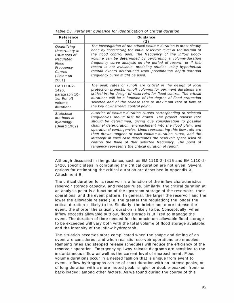
92

Although discussed in the guidance, such as EM 1110-2-1415 and EM 1110-2-1420, specific steps in computing the critical duration are not given. Several options for estimating the critical duration are described in Appendix X, Attachment B.

The critical duration for a reservoir is a function of the inflow characteristics, reservoir storage capacity, and release rules. Similarly, the critical duration at an analysis point is a function of the upstream storage of the reservoirs, their operations, and the event pattern. In general, the larger the reservoir and the lower the allowable release (i.e. the greater the regulation) the longer the critical duration is likely to be. Similarly, the briefer and more intense the event, the shorter the critically duration is likely to be. Conceptually, when inflow exceeds allowable outflow, flood storage is utilized to manage the event. The duration of time needed for the maximum allowable flood storage to be exceeded will vary both with the total volume of flood storage available, and the intensity of the inflow hydrograph.

The situation becomes more complicated when the shape and timing of an event are considered, and when realistic reservoir operations are modeled. Ramping rates and stepped release schedules will reduce the efficiency of the reservoir operation. Emergency spillway release diagrams are sensitive to the instantaneous inflow as well as the current level of encroachment. Flood volume durations occur in a nested fashion that is unique from event to event. Inflow hydrographs can be of short duration with an intense peaks, or of long duration with a more muted peak; single- or double-peaked; front- or back-loaded; among other factors. As we found during the course of this

Table 13. Pertinent guidance for identification of critical duration Reference

(1) Guidance

(2) Quantifying Uncertainty in Estimates of Regulated Flood Frequency Curves (Goldman 2001)

The investigation of the critical volume-duration is most simply done by considering the initial reservoir level at the bottom of the flood control pool. The frequency of the inflow flood-volume can be determined by performing a volume-duration frequency curve analysis on the period of record; or if this record is not available, modeling studies using hypothetical rainfall events determined from precipitation depth-duration frequency curve might be used.

EM 1110-2-1420, paragraph 10-1c: Runoff volume durations

The peak rates of runoff are critical in the design of local protection projects, runoff volumes for pertinent durations are critical in the design of reservoirs for flood control. The critical durations will be a function of the degree of flood protection selected and of the release rate or maximum rate of flow at the key downstream control point.

Statistical methods in hydrology (Beard 1962)

A series of volume-duration curves corresponding to selected frequencies should first be drawn. The project release rate should be determined, giving due consideration to possible channel deterioration, encroachment into the flood plain, and operational contingencies. Lines representing this flow rate are then drawn tangent to each volume-duration curve, and the intercept in each case determines the reservoir space used to control the flood of that selected frequency. The point of tangency represents the critical duration of runoff.

93

study, although a single critical duration is often used to characterize a reservoir or regulated system, in reality the duration of unregulated volume that causes a regulated peak flow can and will vary as a function of both the size and shape of an event in addition to the characteristics of the regulated system.

For completely unregulated watersheds the critical duration assessment is not required as there is no difference between the unregulated and regulated flow hydrographs.

Study procedure

The duration used to relate the annual exceedence probability to the peak flow from the unregulated flow-duration-frequency curve (volume frequency curve) varies by scale factor and historical-event pattern. This “critical duration” is associated with the volume of water found to drive the peak regulated flow at that location based on reservoir operations and channel routing. The method to find this duration, referred to as the “volume window method” as well as additional issues and procedural information on the development of this transform are found in Appendix X. The volume-window method relates the timing of the peak regulated outflow to the maximum n-day volumes for an event. By quantifying the proximity of the event maximum unregulated volume to the peak regulated flow, the duration most closely related to the regulated peak may be identified. Unlike the more simplified methods described in the guidance above, the complexities of reservoir operations and event size, shape and timing are accounted for. But, as opposed to the statistical correlation methods initially considered for use in this study, the focus on the causal relationship between the unregulated flow volume and regulated peak is preserved, which in the experience of the study team significantly reduces the probability of mis-identifying the critical duration. .

Fitting a “most likely” transform through the datasets Situation

After completing the required model runs and extracting the data pairs, a “most-likely” curve must be fit. This curve translates the unregulated flow of a given quantile to the corresponding regulated flow for that same quantile. Likewise, this curve translates a regulated flow at an analysis point to a water level. Thus, the final regulated flow-frequency curve is sensitive to the shape and fit of this curve.


The guidance pertinent to fitting the transform is listed in EM 1110-2-1415 section 3-9d, paragraph (1b) which states:

The frequency of reservoir outflows or of flows at a downstream location can be obtained from routings of the period-of-record runoff by the following method(s): Construct a graph of with-project versus without-project flows at the location of interest and draw a curve relating the two quantities...

The points should be balanced in the direction transverse to the curve, but factors such as flood volume of events and reliability

94

of regulation must be considered in drawing the curve. This curve can be used in conjunction with a frequency curve of without-project flows to construct a frequency curve of with-project flows...

This latter procedure assures consistency in the analysis and gives a graphical presentation of the variability of the regulated events for a given unregulated flow.

Based on a review of the literature and previous studies, various options for fitting the “most likely” curve through the datasets have been used. For the CVHS, the method used should satisfy the following criteria:

Does the method capture the inflection points of the datasets?

Does the method promote consistency through a reach (from analysis point to analysis point)?

Does the method maintain a positive slope (i.e. the unregulated-regulated transform is never inversely proportional.)?

Study procedure

For a given pattern, a collection of flow pairs are generated by simulating scaled versions of the event. Each scaling results in an unregulated volume corresponding to the critical duration, and a regulated peak flow. An event-specific unregulated to regulated transform is generated by connecting (interpolating between) flow pairs.

With an unregulated to regulated transform defined for each event, an event-specific regulated frequency curve is obtained by plotting the regulated peak flow values against probability. The result is a shape-specific (conditional) regulated frequency curve for each event pattern. There is only one regulated frequency curve at a given location. Therefore, the event-specific regulated frequency curves must be combined to obtain a single regulated frequency curve. In the general case, if all patterns capable of producing a regulated flow value of interest are accounted for, and the relative likelihoods of these events producing that regulated flow are known, then the total probability theorem is applied to compute the probability associated with the regulated flow value

The relative likelihood of an event producing a large regulated flow can be estimated from the inverse of the exceedance probability of the historical (unscaled) event. The exceedance probability of an event, historical or scaled, is obtained from the unregulated volume frequency curve corresponding to the critical duration of the event. The inverse of the exceedance probability for each event is then normalized such that the sum of all event patterns is equal to one, yielding the relative likelihood of each event pattern. In effect, when the total probability theorem is applied, these relative likelihoods can be thought of as the “weights” used to compute an average or most likely curve.With the selected approach, a single continuous regulated frequency curve is defined only for the probability range for which all event-specific regulated frequency curves are defined.

95

Since the process of transforming the unregulated flow-duration-frequency curve does not require a single critical duration to be used across all historical patterns and scale factors, a single unregulated flow to regulated flow transform isn’t explicitly developed and applied. However, if needed, the predominant duration found through that analysis could be “backed out” and plotted for quick evaluations.During the process described above, various measures are taken to retain consistency in the analysis. Thus, in some cases, the process may require a few iterations before the final regulated flow-frequency curve is ready to be adopted for the study. Some of these measures include:

Verifying that in the event-specific regulated flow frequency curve, with decreasing annual exceedence probability the peak regulated flow does not decrease. For these cases, the critical durations are typically re-examined, or the curve adjusted directly.

Verifying consistency and trends amongst the critical duration for specific event patterns. Although the critical durations do not need to remain constant for a given historical pattern, we expect to see a basic trend in critical duration with increasing scale factor. For cases where this does not occur, the calculations and simulations are reviewed and adjustments made if appropriate.

Verifying consistency in the weighting of historical patterns, for the combining of the event-specific curves, as you move through the system. Again, although not a requirement, the weights are reviewed and inspected for trends, making modifications when appropriate.

Details of this process are described in Appendix X.

Once the regulated curves are reviewed and refined, they are accepted for the study.

96

Results The results of this frequency analysis include:

Unregulated frequency curves for floods-of-record analysis points (as shown in Appendix VII.

Regulated flow-frequency curves and associated volumes for floods-of-record analysis points (as shown in Appendix X).

Flow-frequency curves for the “Task 8” watershed analysis points (as provided in Appendix XI).

97

Lessons learned and cautionary notes Every study has both strengths and weaknesses. We believe the CVHS represents a large step forward with respect to characterizing the flood risk in the Central Valley. Key strengths include: an ability to incorporate the variability of natural flood patterns, both on a temporal and spatial scale; development and application of the next generation of hydrologic and hydraulic models to evaluate both regulated and unregulated conditions; generation of a system wide set of unregulated boundary conditions over the period of record that in many ways maximizes the utilization of available streamflow data; and an updated set of unregulated flow frequency estimates using the best available data and methodology.

A great deal of thought and effort was put into developing the procedures to be used in the CVHS before any analysis was performed. This included drawing upon the available guidance, previous studies both within and without the study area, and consultation of leading experts in the field to assess the proposed methods of analysis. During application, some of these procedures needed to be reconsidered and modified, in response to issues that arose applying them to the unique hydrology of the Central Valley, which is remarkable both in terms of range of natural hydrologic variability, and the complexity of the existing flood management system.

As would be expected for any effort of this magnitude, during the course of this study a number of lessons were learned by the analysts, which we would like to share. Additionally, we feel that certain details should be brought to the attention of potential users of the study products and methods, to ensure proper use and application:

A first application of CVHS procedures selected 20-30 historic events to develop the unregulated-regulated transform. This resulted in a great deal of scatter in the resulting transform data set, which in hindsight did not result in a reliable characterization of the regulated system. The primary problem with this approach is the scarcity of historic events that are truly representative of the type of storm that would be expected to stress the flood control system. Simply scaling up a more common event from the historic record to the magnitude of a rare flood does not reliably result in realistic reservoir inflows or coincident local flow patterns in the resulting simulation. We found that we have much more confidence in a transform developed from the largest 3-5 events in the historic record.

Application of the original selected procedure for critical duration assessment, which looked at a variety of events and scaled event patterns and used a correlation statistic to identify the unregulated flow duration most strongly associated with the regulated peak, led to critical duration selections that could not be justified from a physical hydrology or reservoir operations perspective. Instead, a new approach was developed that drew upon previous work by Leo Beard, and others, in assessing the cause and effect relationship between an unregulated volume and the response of a regulated system. Again, we believe the problem does not lie with the details of the original method in itself, but instead with the lack of sufficient data to properly and reliably apply the method to the Central Valley. There are simply not enough examples of large floods in the systematic record to adequately assess the response of the regulated

98

system to a variety of hydrograph shapes and durations of varying magnitude.

Among the noted strengths of the CVHS procedure, is that a variety a natural storm patterns, which includes a variety of natural storm centerings and temporal distributions, are analyzed. However, the method used to scale these historic events, both up and down, throughout the system does have limitations: simply applying uniform scale factors to boundary condition flows throughout the system does not perfectly preserve historic event flow probability relationships. The natural variability in flow frequency characteristics across the Central Valley is impressive: for a single duration (1-day), computed log10 standard deviations range from 0.23 to 0.55, and adopted log10 skews from -0.7 to +0.1. There is also considerable variability across durations at a single location. As a result of this variability in flow frequency, scaling all of the boundary conditions by a single linear factor has the potential to distort the natural spatial and temporal patterns inherent in the original unscaled event. It is hoped that in the future more sophisticated methods for scaling historic floods will be developed to address this limitation.

Due to the original scope of this study, regulated flow frequency curves have been developed for in-channel flows only. However, these curves do not always tell the complete story of what is happening in the system. Especially in the San Joaquin Basin, there may be significant overbank flow occurring simultaneously, either from flow exiting the levee system upstream, or from a nearby tributary. At a minimum, when modeling an event selected from an in-channel curve, boundary conditions should be carefully selected such that all significant sources of flow into the study area are accounted for. Ideally, at-latitude regulated flow frequency curves (or, alternatively, stage-frequency curves) could be developed at locations where this out of bank flow component is significant.

As has been emphasized repeatedly throughout this report, regulated system modeling assumptions should be examined before adopting “go-by” products. There simply is no “one-size-fits-all” approach to modeling a regulated system as complex as the Sacramento and San Joaquin Basins. By modeling “by the book” operations using relatively conservative initial storage assumptions, we hope to have realistically modeled the system response to the rare floods that are the focus of this study. These assumptions are more questionable for more routine storm events, for which additional incidental flood space is often available, and for which projected water supply demand is often sufficient to empty a reservoir’s flood pool without resorting to aggressive flood releases. Even for the rarest floods of record, such as 1986 and 1997, actual operations will often vary significantly from our simplified assumptions, as the full capacity of the system is used to efficiently manage the flood event in a way that has not been spelled out in individual project’s water control manuals. Levee fragility and performance represent another area for which significant variability exists and for which a relatively simple assumption was adopted for this analysis. More focused applications in the future will have the opportunity to re-examine and potentially revise these assumptions to a degree that is simply not possible in a watershed study of this scale. We recommend that historic data be examined for more

99

common events, and our modeling assumptions be examined for more rare events, before these results are adopted for any local application.

The procedures used for the CVHS were initially developed with an objective of developing regulatory flood plains with a high degree of confidence and defensibility. While this level of detail may be appropriate for some applications, such as the final design of a flood risk management measure, this is a standard that may simply not be realistic for other applications, such as reconnaissance or feasibility level analyses. Simplified approaches may be necessary for these applications, especially given the new SMART Planning paradigm that has been adopted by the Corps during the course of this study. For example, it may not be feasible to apply the floods-of-record approach to every alternative under consideration in feasibility study. This is especially the case when you consider that the adopted critical duration selection method is a function of the regulated system, and could therefore be expected to vary with each structural or operational alternative. Fortunately, we believe that it will be possible to leverage the work that has already been done for the existing condition to develop reasonable simplifying assumptions that could be applied when screening alternatives for a planning study.

100

Future work The aforementioned tasks described are required for completing the scope of work given to the Corps by DWR. In the future, the data, information, and tools may be used to refine or enhance the study results or to expand the use of these results for other purposes. Here, we identify ways the procedure and/or products could be refined or modified in the future:

Coordinate with DWR the incorporation of downstream tidal boundary effects into the study procedures.

Further development of tools and documentation to facilitate alternative analyses.

Update study results, specifically development of the regulated flow time series and the subsequent steps, using newly-developed regulated condition channel models from the CVFED effort. Currently, DWR contractors are developing a new regulated condition channel model based on the latest topographic data and levee geometry. Once completed, these channel models can be used to route the historical and scaled historical events to refine the unregulated-regulated flow transform and the flow-stage transform.

Update study results with additional years of record. With time and with a properly funded gage network, we will have additional years of data with which to update the hydrologic analysis results. The first step in this update is to extend the unregulated flow time series to include the new records. The second step in such an update would be to re-analyze the flow-frequency curves using the updated time series. As needed, the regional skew values could also be updated based on the additional years of data. Finally, the extended record length could be used to develop more data points for the unregulated-regulated flow transform and adjust the curve, if necessary.

Increase resolution of boundary conditions. At present, the upstream boundary condition for the modeling was defined based on the required study area. Thus, the upstream boundary conditions were set, for the most part, at the project reservoirs. If needed, additional work could be completed to start the unregulated flow time series above the project reservoirs. Further, if additional stream gages are added to the system, then those collected data may be useful for increasing the spatial resolution of the boundary condition locations.

Consider the use of wetness indices for reservoir simulation to adapt CVHS procedures for water supply applications. For flood control reservoirs having variable top of conservation during the rain season, historical basin wetness could be used to derive a historically-based top of conservation. This refinement could only be available in years in which required data to compute the index were available. In earlier years, an average, or maximum wetness could be adopted.

Consider the sensitivity of channel routing assumptions, most notably the sensitivity of the system levee performance assumption. For the CVHS, the assumption that levees overtop but do not fail is used for development of the regulated flow time series. This assumption was made as it represents a physical condition. However, the CVHS team does not state

101

an opinion on the likelihood of this reflecting reality or that it is the appropriate assumption for other applications. In other work, the sensitivity of this assumption, as compared to levee failure at overtopping, for example, could be assessed and compared.

Develop confidence bounds about the unregulated-regulated and flow-stage transform. Under the current DWR-Corps LOA, the CVHS team is charged with describing sources of uncertainty in the completed hydrology, but not to develop confidence bounds about the study results. Using the models and information developed in the study, additional work could be completed to refine the results within a risk and uncertainty framework, and thus develop relationships with uncertainty bounds. These products could then be used to support levee certification, risk and uncertainty analysis, and other such studies. Included in the Product uses document is an example of how this could be done.

Complete and apply snowmelt regional skew analysis, and develop snowmelt flow frequency curves. Here, regional skew values corresponding to peak flows and various durations could be developed from snowmelt flood events. These values could then be used to improve the consistency of the more frequent events of the total probably curve, especially for the San Joaquin Basin.

Evaluate the effect of various climate change scenarios on the study products. For this, consider the impact on variations of precipitation patterns and/or evaluate trends in the historical record. For the former, use, for example, watershed models to evaluate how a smaller snow pack could affect future runoff events and the downstream regulated flows. For the latter, use, for example, a subset of the historical record for the last 50 years and evaluate the potential change in the frequency curves.

Develop seasonal flow frequency curves, to be used when scaling spring and fall flood events which would allow for evaluation of flood risk during the drawdown and refill portions of a seasonal Water Control Diagram.

Incorporate uncertainty into the reservoir operation simulations, including contingency factors to account for uncertainty in the local flow estimation.

Develop confidence limits on unregulated flow frequency curves, especially those developed using EMA and MGB, to be used in HEC-FDA for USACE Planning Studies. This will require coordination between the Sacramento District and the USACE Hydrologic Engineering Center.

Develop alternate methods for scaling boundary conditions, to better preserve the complex physical and probabilistic relationships existing between the various watersheds in the Central Valley.

102

References Beard, Leo R. (1962). Statistical methods in hydrology. Hydrologic

Engineering Center, US Army Corps of Engineers, Davis, CA.

Bradley, Allen A. Jr., and Potter, Kenneth W. (2004). PVSTATS, user manual version 3.1. University of Wisconsin-Madison, Department of Civil and Environmental Engineering, Madison, WI.

Cleveland, William S. (1979). “Robust locally weighted regression and smoothing scatter plots.” Journal of the American Statistical Association, 74(368) 829-836.

Cohn, Tim. (2007). PeakfqSA, version 0.937 [Software]. <http://www.timcohn.com/TAC_Software/PeakfqSA/>.

Goldman, David M. (2001). “Quantifying uncertainty in estimates of regulated flood frequency curves.” State of the practice – proceedings of the World Water and Environmental Resources Congress, ASCE, Reston, VA.

Helsel, D. R., and Hirsch, R. M. (2002). Statistical methods in water resources, US Geological Survey, Reston, VA.

Hundley, Norris Jr., (1992) The Great Thirst: Californians and Water, 1770s-1990s , University of California Press.

Interagency Advisory Committee on Water Data (IACWD). (1982). Guidelines for determining flood flow frequency, Bulletin 17B. US Geological Survey, Reston, VA.

US Army Corps of Engineers (USACE). (1983). New Hogan Dam and Lake, Calaveras River, California, Water control manual, Appendix III to Master water control manual, San Joaquin River Basin, California, Sacramento District, Sacramento, CA.

USACE. (1990). Calaveras River, California: Reconnaissance report, Sacramento District, Sacramento, CA.

USACE. (1993). Hydrologic frequency analysis, EM 1110-2-1415, Washington, D.C.

USACE. (1994). Engineering and design-hydrologic engineering studies design, EP 1110-2-9, Washington, D.C.

USACE. (1997). Hydrologic engineering requirements for reservoirs, EM 1110-2-1420, Washington, D.C.

USACE. (2002a). Sacramento and San Joaquin river basins comprehensive study, December 2002 interim report (“Comp study”), USACE, Sacramento District, Sacramento, CA.

USACE (2002b). Sacramento and San Joaquin river basins comprehensive study, Technical studies documentation, Appendix B: Synthetic hydrology technical documentation.

USACE (2002c). Sacramento and San Joaquin river basins comprehensive study, Technical studies documentation, Appendix C: Reservoir operations modeling, existing design operations and reoperation analyses. Available at

103

USACE. (2004). Farmington Dam and Reservoir, Littlejohn Creek, California, Water control manual, Appendix IV to Master water control manual, San Joaquin River Basin, California, Sacramento District, Sacramento, CA.

USACE. (2009a). Central Valley hydrology study (CVHS): Technical procedures document (“Technical procedures document”), prepared by David Ford Consulting Engineers, Inc., Sacramento, CA.

USACE. (2009b). CVHS product uses (“Uses document”), prepared by David Ford Consulting Engineers, Inc., Sacramento, CA.

USACE. (2009c). Sacramento and San Joaquin river basins: Procedures for hydrologic analysis (“Procedures document”), prepared by David Ford Consulting Engineers, Inc., Sacramento, CA.

USACE. (2010). Hydrologic engineering management plan for the Lower San Joaquin River feasibility study, prepared by David Ford Consulting Engineers, Inc., Sacramento, CA.

USACE. (2011a). Central Valley hydrology study (CVHS): Technical procedures document, prepared by David Ford Consulting Engineers, Inc., Sacramento, CA.

USACE. (2011b). Central Valley hydrology study (CVHS) technical procedures document Appendix B: Unregulated time series development, prepared by David Ford Consulting Engineers, Inc., Sacramento, CA.

USACE. (2011c). Central Valley hydrology study (CVHS) Technical procedures document Appendix C: Regulated time series development, prepared by David Ford Consulting Engineers, Inc., Sacramento, CA.

USACE. (2011d). Central Valley hydrology study (CVHS) Technical procedures document Appendix D: Flow frequency analysis, prepared by David Ford Consulting Engineers, Inc., Sacramento, CA.

USACE. (2011e). Central Valley hydrology study (CVHS) Technical procedures document Appendix E, Development of flow and stage transforms, prepared by David Ford Consulting Engineers, Inc., Sacramento, CA.

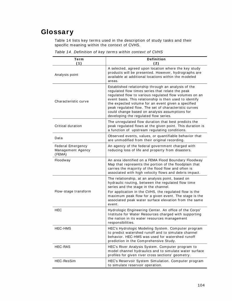
104

Glossary Table 14 lists key terms used in the description of study tasks and their specific meaning within the context of CVHS.

Table 14. Definition of key terms within context of CVHS

Term (1)

Definition (2)

Analysis point

A selected, agreed upon location where the key study products will be presented. However, hydrographs are available at additional locations within the modeled areas.

Characteristic curve

Established relationship through an analysis of the regulated flow times series that relate the peak regulated flow to various regulated flow volumes on an event basis. This relationship is then used to identify the expected volume for an event given a specified peak regulated flow. The set of characteristic curves could change based on analysis assumptions for developing the regulated flow series.

Critical duration The unregulated flow duration that best predicts the peak regulated flows at the given point. This duration is a function of upstream regulating conditions.

Data Observed events, values, or quantifiable behavior that are unmodified from their original recording.

Federal Emergency Management Agency (FEMA)

An agency of the federal government charged with reducing loss of life and property from disasters.

Floodway An area identified on a FEMA Flood Boundary Floodway Map that represents the portion of the floodplain that carries the majority of the flood flow and often is associated with high velocity flows and debris impact.

Flow-stage transform

The relationship, at an analysis point, based on hydraulic routing, between the regulated flow time series and the stage in the channel. For application in the CVHS, the regulated flow is the maximum peak flow for a given event. The stage is the associated peak water surface elevation from the same event.

HEC Hydrologic Engineering Center. An office of the Corps’ Institute for Water Resources charged with supporting the nation in its water resources management responsibilities.

HEC-HMS HEC’s Hydrologic Modeling System. Computer program to predict watershed runoff and to simulate channel behavior. HEC-HMS was used for watershed runoff prediction in the Comprehensive Study.

HEC-RAS HEC’s River Analysis System. Computer program to model channel hydraulics and to simulate water surface profiles for given river cross sections’ geometry.

HEC-ResSim HEC’s Reservoir System Simulation. Computer program to simulate reservoir operation.

105

Term (1)

Definition (2)

information The results of applying tools or processes to data.

National Flood Insurance Program (NFIP)

.A program of the federal government that subsidizes insurance for properties in designated floodplains.

National Weather Service (NWS)

Part of the Department of Commerce, National Oceanic and Atmospheric Administration (NOAA). The federal governmental agency that provides weather, hydrologic, and climate forecasts and warnings for the United States.

Observed Obtained through the senses or by instrumentation for measuring condition or state.

Regulated flow

Change in a river’s natural flow due to the influence of hydraulic constriction(s) or manmade influence(s). In this study, regulated flow is the modified unregulated flow (see below) due to reservoir storage, overbank storage as a result of levee overtopping and/or failure, and the effect of bridges and hydraulic structures. The same channel alignment as used in the unregulated flow development is used here. It does not specifically include, or account for, land use changes.

Regulated flow time series

The time series that is the result of adding back the effects of reservoirs, off stream storage (both planned as in the case of diversions and unplanned as in the case of a levee failure), and other system features represented in the regulated channel model (but not in the unregulated channel model). This is discussed in Appendix VIII.

Regulated system

The flood control system, including reservoirs, channels, levees, and bypasses. This condition is sometimes referred to as the with-project condition.

Results Information that is the output from a toolset or process.

Simulated Developed through the use of a computer program designed to model hydrology, hydraulics, reservoir operation, etc.

State of California Department of Water Resources (DWR)

A unit of the California state government responsible for various regulatory functions regarding water supply, water use, and flood management.

106

Term (1)

Definition (2)

Unregulated flow

A modification of the historical flow set that can be used as the basis of a flood-flow-frequency analysis consistent with the requirements of Bulletin 17B. For application in the CVHS, the unregulated condition corresponds to the absence of reservoir and overbank storage. This is similar to “unimpaired flows” and “full natural flows” as used in DWR planning activities, but focuses more on the largest event rather than smaller events. For example, less emphasis is put on the low flow periods of the year for this flood analysis than may be for a water supply or environmental functions analysis. Further, here, the unregulated flow still includes an effect of the flow constrictions due to the channelization of the streams. Therefore unregulated flows in the CHVS are not necessarily the same as the “unimpaired flows” and “full natural flows” as used by DWR.

Unregulated flow time series

The time series that is constructed by routing the unregulated reservoir inflows and adding the estimated local flows into the system. The time series represents the maximum potential flow delivery and is sufficient for fitting statistical relationships. This is discussed in more detail in Appendix III.

Unregulated system

The stream system and model used to develop the unregulated flow time series. Outside of Corps planning usage, this condition is sometimes referred to as the without-project condition. (Within Corps planning usage, this term has a more specific meaning.)

US Army Corps of Engineers (Corps or USACE)

An agency of the US Army that serves the armed forces and the nation by providing engineering services and capabilities across a spectrum of operations in support of the national interest. Corps missions include five broad areas: water resources, environment, infrastructure, homeland security, and warfighting.

US Geological Survey (USGS)

Part of the Department of the Interior. The sole science agency for the Department of the Interior, serving as an independent fact-finding agency that collects, monitors, analyzes, and provides scientific understanding about natural resource conditions, issues, and problems.

107

Supplemental resources Throughout the study, we have prepared detailed documentation, which is supplemental to this report. Table 15 lists the documentation. The documentation is available for download from the CVHS Web forum, www.cvhydrology.org (username: CVHS_GEN, password: featherriver).

Table 15. Supplemental resources

ID (1)

Document (2)

Date (3)

Description (4)

1 Procedures for Hydrologic Analysis (“Procedures document”)

9/9/2008 Describes methods and procedures employed in the study. Sets the context of the study and serves as the study Hydrologic Engineering Management Plan (HEMP).

2 CVHS Product Uses

5/20/2009 Provides a description of CVHS products and how they can be used for a range of applications. These applications include delineating floodplains using either a single reach channel model or a multi-reach channel model.

3 Life After Central Valley Hydrology Study

12/1/2010 Describes procedure for using CVHS to develop hydrologic and hydraulic information for planning/risk analysis studies.

4 Technical procedures document

4/8/2011 Describes methods and procedures employed in the study.

5 Ungaged Watershed Analysis Procedures

11/15/2011 Describes the process of developing required information for the ungaged watersheds, including the flow frequency curves.

6 Unregulated Rain-flood Frequency Curves Analysis Description

12/6/2012 Describes development of the unregulated flow frequency curves.

7 Regulated Frequency Curve Method

2/8/2013 Describes procedures used for an application of CVHS, where regulated flow frequency curves were developed for specific levee performance conditions.

8 Interim work product technical memoranda

2013 Provides details on study procedures and interim results and findings.

9 Interim work product sensitivity analysis reporting

2013 Describes various sensitivity analyses and comparisons to past studies that have been completed throughout the study.

10 Task 8 rainfall-runoff analysis reports

2013, 2014 Describes rainfall-runoff analyses and results for the CVHS Task 8 watersheds.

108

ID (1)

Document (2)

Date (3)

Description (4)

11 Application of CVHS Regulated Frequency Curve Methods to the Sacramento Basin Existing “Top-of-Levee” (TOL) Condition

5/23/2014 Describes procedures used for an application of CVHS, where regulated flow frequency curves were developed for specific levee performance conditions.

109

Contributors to study

Study team Department of Water Resources

Jon Ericson

Sudhakar Talanki

Mitch Russo

Binta Coleman

MD Hague

US Army Corps of Engineers

John High

Brad Moore

Rob Thompson

Bob Collins

Brian Walker

Angela Duren

Bill Curry

David Ho

Jim Mars

Kim Carsell, Proj Mgr

Judy Soutierre, Proj Mgr

Mellisa Hallas, Proj Mgr

David Ford Consulting Engineers, Inc (Consultant to US Army Corps of Engineers)

David Ford

Nathan Pingel

US Geological Survey

Charles Parrett

Justin Ferris

110

Study review team The following agencies provided technical review of portions of the analysis.

Review of Procedures: HEC Staff (Jeff Harris) and Dr. David Goldman, and the Hydrologic Advisory Committee

ATR of Task 8 rainfall-runoff modeling: HEC Staff (Matt Fleming and Jay Pak)

ATR of Unregulated Flow Frequency Curves: Dr. David Goldman

ATR of HEC-ResSim Models: Dan Barcellos

Hydrologic advisory committee: (Jay Lund of UC Davis, Daene McKinney of University of Texas, Austin, Jery Stedinger of Cornell University)

Acknowledgements The study team appreciates the support and cooperation, through various conversations, discussions, and reviews, of the following agencies and individuals:

Hydrologic Engineering Center (HEC): Dr. Beth Faber, Chris Dunn, Matt McPherson, Jeff Harris, Chan Modini, Dan Barcellos, and others

FEMA Region 9 (Kathy Schaeffer)

USGS (Charles Parrett, Justin Ferris)

NOAA (Hydrometeorological Design Studies Center in Silver Springs, MD)

MBK Engineers (Joe Countryman, PE and Ben Tustison, PE)

However, the support these persons do not imply endorsement of the results presented.

111

Appendix I. Analysis points Refer to Appendix_I_Analysis_Points.pdf.

112

Appendix II. Summary of computer model development and uses

Refer to Appendix_II_Computer_Models.pdf.

113

Appendix III. Flow time series development and documentation

Refer to Appendix_III_Flow_Time_Series.pdf.

114

Appendix IV. Completed unregulated flow time series

Refer to Appendix_IV_Completed_Unregulated_Flows.pdf.

115

Appendix V. Annual maximum series for frequency analysis

Refer to Appendix_V_Annual_Series_for_Freq_Analysis.pdf.

116

Appendix VI. Unregulated flow-frequency analysis

Refer to Appendix_VI_Unregulated_Flow-Freq_Analysis.pdf.

117

Appendix VII. Unregulated flow-frequency curves

Refer to Appendix_VII_Unregulated_Flow-Frequency_Curves.pdf

118

Appendix VIII. Completed regulated flow times series

Refer to Appendix_VIII_Regulated_Flow_Time_Series.pdf.

119

Appendix IX. Extracted event dataset Refer to Appendix_IX_Extracted_Event_Dataset.pdf.

120

Appendix X: Development and application of unregulated-regulated flow transform

Refer to Appendix_X_Transforms_and_Critical_Duration.pdf.

121

Appendix XI. Rainfall-runoff modeling Refer to Appendix_XI_Raninfall-Runoff_Modeling.pdf.

central valley hydrology study - ford...

Documents