cellular learning automata with multiple learning automata...

Cellular Learning Automata with Multiple Learning Automata

in Each Cell and its Applications

1 Hamid BeigyDepartment of Computer Engineering,

Sharif University of Technology,Tehran, Iran

[email protected]

and2 M. R. Meybodi

Computer Engineering and Information Technology Department,Amirkabir University of Technology,

Tehran, [email protected]

Abstract. The cellular learning automata, which is a combination of cellular automata and learn-ing automata, is introduced recently. This model is superior to cellular automata because of itsability to learn and also is superior to single learning automaton because it is a collection of learn-ing automata which can interact with each other. The basic idea of cellular learning automata is touse the learning automata to adjust the state transition probability of stochastic cellular automata.Recently, various types of cellular learning automata such as synchronous, asynchronous, and opencellular learning automata have been introduced. In some applications such as cellular networks weneed to have a model of cellular learning automata for which multiple learning automata residesin each cell. In this paper, we study a cellular learning automata model for which each cell hasseveral learning automata. It is shown that for a class of rules, called commutative rules, the cellu-lar learning automata converges to a stable and compatible configuration. Two applications of thisnew model such as channel assignment in cellular mobile networks and function optimization arealso given. For both applications, it has been shown through computer simulations that the cellularlearning automata based solutions produce better results.

1 Introduction

Cellular automata (CA) are mathematical models for systems consisting of large numbers of simpleidentical components with local interactions. The simple components act together to produce complexemergent global of behavior. Cellular automata perform complex computation with high degree of effi-ciency and robustness. They are specially suitable for modelings natural systems that can be describedas massive collections of simple objects interacting locally with each other [1]. Cellular automata calledcellular, because it is made up cells like points in the lattice and it called automata, because it followsa simple local rule [2]. Each cell can assume a state from finite set of states. The cells update theirstates synchronously on discrete steps according to a local rule. The new state of each cell depends onthe previous states of a set of cells, including the cell itself, and constitutes its neighborhood [3]. Thestate of all cells in the lattice are described by a configuration. A configuration can be described as thestate of the whole lattice. The rule and the initial configuration of the CA specifies the evolution of CAthat tells how each configuration is changed in one step. On other hand, learning automata (LA) are,by design, ”simple agents for doing simple things”. Learning automata have been used successfully inmany applications such as control of broadcast networks [4], intrusion detection in sensor networks [5],database systems [6], and solving shortest path problem in stochastic networks [7, 8], to mention a few.The full potential of a LA is realized when multiple automata interact with each other. Interaction mayassume different forms such as tree, mesh, array and etc. Depending on the problem that needs to besolved, one of these structures for interaction may be chosen. In most applications, local interaction ofLAs, which can be defined in a form of graph such as tree, mesh, or array, is more suitable. In [9], CAand LA is combined and a new model which is called cellular learning automata (CLA) is obtained. This

2 Hamid Beigy and M. R. Meybodi

model, which opens a new learning paradigm, is superior to CA because of its ability to learn and also issuperior to single LA because it is a collection of LAs which can interact with each other.

The CLA can be classified into two groups : synchronous and asynchronous CLA [10]. In synchronousCLA, all cells are synchronized with a global clock and executed at the same time and in asynchronousCLA, LAs in different cells are activated asynchronously. The CLA can be classified into close and open[11]. In the former, the action of each learning automaton in next stage of its evolution only depends onthe state of its local environment (actions of its neighboring LAs) while in the later, the action of eachlearning automaton in next stage of its evolution not only depends on the local environment but it alsodepends on the external environments.

In [12], a mathematical framework for studying the behavior of the CLA has been introduced. Thismathematical framework for the CLA not only enables us to investigate the characteristics of this modeldeeper, which may lead us to find more applications, but having such a mathematical framework alsomakes it possible to study the previous applications more rigorously and develop better CLA basedalgorithms for those applications. In [11], open cellular learning automata has been introduced and itssteady state behavior was studied. Asynchronous cellular automata was proposed in [10] and its steadystate behavior was studied. In [10–12], the steady state behavior of different models of CLA are studiedand it was shown that for a class of rules called commutative rules, the CLA converges to a globally stablestate. The CLA have been used in many applications such as image processing [13], rumor diffusion [14],modelling of commerce networks [15], channel assignment in cellular networks [16], call admission controlin cellular networks [10], and sensor networks [17] to mention a few.

In some applications such as channel assignment in cellular networks, a type of cellular learningautomata is needed such that each cell is equipped multiple LAs. The process of assignment of channelsto a cell or a call depends on the states of the neighboring cells. The state of each cell is determinedby determining the values of several variables. The value of each variable is adaptively determined bya learning automaton assigned to that variable. We call such a CLA as CLA with multiple learningautomata in each cell. In this paper, CLA with multiple LAs in each cell is introduced and its steadystate behavior is studied. It is shown that for commutative rules, this new model converges to a globallystable and compatible configuration. Then two applications of this new model to cellular mobile networksand evolutionary computation have been presented.

The rest of this paper is organized as follows. Section 2 presents a review of studies of the steady statebehavior of synchronous, asynchronous, and open CLA. In section 3, the CLA with multiple learningautomata in each cell is introduced and its behavior is studied. Section 4 presents two applications ofthe proposed model to the channel assignment in cellular networks and function optimization. Section 5presents the computer experiments and section 6 concludes the paper.

2 Cellular learning automata

Cellular learning automata (CLA) is a mathematical model for dynamical complex systems that consistsof a large number of simple components. The simple components, which have learning capability, acttogether to produce complex emergent global behavior. A CLA is a CA in which a learning automatonis assigned to every cell. The learning automaton residing in a particular cell determines its state(action)on the basis of its action probability vector. Like CA, there is a rule that the CLA operate under it. Therule of the CLA and the actions selected by the neighboring LAs of any particular LA determine thereinforcement signal to the LA residing in a cell. The neighboring LAs of any particular LA constitutethe local environment of that cell. The local environment of a cell is nonstationary because the actionprobability vectors of the neighboring LAs vary during evolution of the CLA. In the following subsections,we review some recent results regarding various types of cellular learning automata.

2.1 Synchronous cellular learning automata

In synchronous cellular learning automata, all cells are synchronized with a global clock and executedat the same time. Formally, a d−dimensional synchronous cellular learning automata with n cells is astructure A = (Zd, Φ, A, N,F), where Zd is a lattice of d−tuples of integer numbers, Φ is a finite setof states, A is the set of LAs each of which is assigned to one cell of the CLA, N = {x̄1, x̄2, · · · , x̄m̄} is

Cellular Learning Automata with Multiple Learning Automata in Each Cell and its Applications 3

a finite subset of Zd called neighborhood vector, and F : Φm̄ → β is the local rule of the CLA, whereβ is the set of values that the reinforcement signal can take. The local rule computes the reinforcementsignal for each LA based on the actions selected by the neighboring LAs. We assume that, there existsa neighborhood function N̄(u) that maps a cell u to the set of its neighboring cells. We assume that thelearning automaton, Ai, which has a finite action set αi, is associated to cell i (for i = 1, . . . , n) of theCLA. Let the cardinality of αi be mi.

The state of all cells in the lattice are described by a configuration. A configuration of the CLA atstage k is denoted by p(k) = (p′

1(k), p′

2(k), . . . , p′

n(k))′, where p

i(k) = (pi1(k), . . . , pimi(k))′ is the action

probability vector of LA Ai. A configuration p is called deterministic if action probability vector of eachLA is a unit vector; otherwise it is called probabilistic. Hence, the set of all deterministic configurations,K∗, and the set of all probabilistic configurations, K, in CLA are K∗ = {p|piy ∈ {0, 1} ∀y, i}, andK = {p|piy ∈ [0, 1] ∀y, i}, respectively, where

∑y piy = 1 for all i. Every configuration p ∈ K∗ is called

a corner of K.The operation of the CLA take place as the following iterations. At iteration k, each LA chooses an

action. Let αi ∈ αi be the action chosen by Ai. Then all LAs receive a reinforcement signal. Let βi ∈ β bethe reinforcement signal received by Ai. This reinforcement signal is produced by the application of thelocal rule. The higher value of the reinforcement signal means that the chosen action of Ai will receivehigher reward. Since each set αi is finite, the local rule can be represented by a hyper matrix of dimensionsm1 ×m2 × · · · ×mm̄. These n hyper matrices constitute what we call the rule of the CLA. When all ofthese n hyper matrices are equal, the CLA is called uniform; otherwise it is called nonuniform. A rule iscalled commutative if and only if

F i(αi+x̄1 , αi+x̄2 , . . . , αi+x̄m̄) = F i(αi+x̄m̄ , αi+x̄1 , . . . , αi+x̄m̄−1) = . . . = F i(αi+x̄2 , αi+x̄3 , . . . , αi+x̄1). (1)

For the sake of simplicity in presentation, a ruleF i (αi+x̄1 , αi+x̄2 . . . , αi+x̄m̄) is denoted by F i (α1, α2 . . . , αm̄).The application of the local rule to every cell allows transforming a configuration to a new one. The localrule specifies the reward value for each chosen action. The average reward for action r of automaton Ai

for configuration p ∈ K is defined as

dir(p) =∑y2

. . .∑ym̄

F i(r, y2, . . . , ym̄)∏

l∈N̄(i)l �=i

plyl, (2)

and the average reward for learning automaton Ai and the total average reward for the CLA is denotedby Di(p) =

∑r dir(p)pir and D(p) =

∑i Di(p), respectively. A configuration p ∈ K is compatible if∑

r dir(p)pir ≥∑

r dir(p)qir for all configurations q ∈ K and all cells i. The compatibility of a configurationimplies that no learning automaton in CLA have any reason to change its action.

The following theorems state the steady state behavior of CLA when each cell uses LR−I learningalgorithm. Proofs of these Theorems can be found in [12].

Theorem 1. Suppose there is a bounded differential function D : Rm1+···+mm̄ → R such that for someconstant c > 0, ∂D

∂pir(p) = cdir(p) for all i and r. Then CLA for any initial configuration in K −K∗ and

with sufficiently small value of learning parameter (max{a} → 0), always converges to a configuration,that is stable and compatible, where ai is the learning parameter of LA Ai.

Theorem 2. A synchronous CLA, which uses uniform and commutative rule, starting from p(0) ∈ K−K∗

and with sufficiently small value of learning parameter, (max{a} → 0), always converges to a deterministicconfiguration, that is stable and compatible.

If the CLA satisfies the sufficiency conditions needed for Theorems 1 and 2, then the CLA will convergeto a compatible configuration; otherwise the convergence of the CLA to a compatible configurations cannotbe guaranteed and it may exhibit a limit cycle behavior [18].

2.2 Asynchronous cellular learning automata

In synchronous cellular learning automata, all cells are synchronized with a global clock and executedat the same time. In some applications such as call admission control in cellular networks, a type of


cellular learning automata in which LAs in different cells are activated asynchronously (asynchronouscellular learning automata) (ACLA) is needed. LAs may be activated in either time-driven or step-driven manner. In time-driven ACLA, each cell is assumed to have an internal clock which wakes upthe LA associated to that cell. The internal clocks possibly have different time step durations and areasynchronous, i.e. each going at its own speed and do not change time simultaneously. In step-drivenACLA, a cell is selected in fixed or random order. Formally an d−dimensional step–driven ACLA with ncells is a structure 〈Zd, Φ, A, N, F, ρ〉, where Zd is a lattice of d−tuples of integer numbers, Φ is a finite setof states, A is the set of LAs assigned to cells, N = {x̄1, x̄2, · · · , x̄m̄} is neighborhood vector, F : Φm̄ → βis the local rule, and ρ is an n-dimensional vector called activation probability vector, where ρi is theprobability that the LA in cell i (for i = 1, . . . , n) to be activated in each stage.

The operation of ACLA takes place as the following iterations. At iteration k, each LA Ai is activatedwith probability ρi and the activated LAs choose one of their actions. The activated automata use theircurrent actions to execute the rule (computing the reinforcement signal). The actions of neighboring cellsof the activated cell are their most recently selected actions. Let αi ∈ αi and βi ∈ β be the action chosenby the activated and the reinforcement signal received by LA Ai, respectively. The reinforcement signalis produced by the application of local rule F i. Finally, activated LAs update their action probabilityvectors and the process repeats.

The following theorems state the steady state behavior of ACLA when each cell uses LR−I learningalgorithm. Proofs of these Theorems can be found in [10].

Theorem 3. Suppose there is a bounded differential function D : Rm1+···+mm̄ → R such that for someconstant c > 0, ∂D

∂pir(p) = cdir(p) for all i and r, and ρi > 0 for all i. Then ACLA for any initial

configuration in K − K∗ and with sufficiently small value of learning parameter (max{a} → 0), alwaysconverges to a configuration, that is stable and compatible, where ai represents the learning parameter forLA Ai.

Theorem 4. An ACLA, which uses uniform and commutative rule, starting from p(0) ∈ K − K∗ andwith sufficiently small value of learning parameter, (max{a} → 0), always converges to a deterministicconfiguration, that is stable and also compatible.

2.3 Open cellular learning automata

In previous versions of CLA, the neighboring cells of a LA constitutes its neighborhoods and the stateof a cell in the next stage depends only on the states of neighboring cell. In some applications such asimage processing, a type of CLA is needed in which the action of each cell in next stage of its evolutionnot only depends on the local environment (actions of its neighbors) but it also depends on the externalenvironments. This model of CLA is called as open cellular learning automata (OCLA). In OCLA, twotypes of environments are considered: global environment and exclusive environment. Each OCLA hasone global environment that influences all cells and an exclusive environment for each particular cell.

Formally an d−dimensional OCLA with n cells is a structure A = (Zd, Φ, A, EG, EE , N,F), whereZd is a lattice of d−tuples of integer numbers, Φ is a finite set of states, A is the set of LAs each of whichis assigned to each cell, EG is the global environment, EE = {EE

1 , EE2 , . . . , EE

n } is the set of exclusiveenvironments, where EE

i is the exclusive environment for cell i, N = {x̄1, x̄2, · · · , x̄m̄} is neighborhoodvector, F : Φm̄ × O(G) × O(E) → β is the local rule of the OCLA, where O(G) and O(E) is the set ofstates of global and exclusive environments, respectively.

The operation of OCLA takes place as iterations of the following steps. At iteration k, each LA choosesone of its actions. Let αi be the action chosen by LA Ai. The actions of all LAs are applied to their cor-responding local environments (neighboring LAs) as well as global environments and their correspondingexclusive environments. Then all LAs receive their reinforcement signal, which is combination of theresponses from local, global and exclusive environments. These responses are combined using the localrule. Finally, all LAs update their action probability vectors based on the received reinforcement signal.Note that the local environment for each LA is nonstationary while global and exclusive environmentsmay be stationary or nonstationary. We now present the convergence result for the OCLA in stationaryglobal and exclusive environments when each cell uses LR−I learning algorithm. These Theorems ensureconvergence to one compatible configuration if the OCLA has one or more compatible configurations.Proofs of these Theorems can be found in [11].


Theorem 5. Suppose there is a bounded differential function D : Rm1+···+mm̄ × O(G) × O(E) → Rsuch that for some constant c > 0, ∂D

∂pir(p) = cdir(p) for all i and r, and ρi > 0 for all i. Then OCLA

(synchronous or asynchronous) for any initial configuration in K − K∗ and with sufficiently small valueof learning parameter (max{a} → 0), always converges to a configuration, that is stable and compatible,where ai is the learning parameter of LA Ai.

Theorem 6. An OCLA (synchronous or asynchronous), which uses uniform and commutative rule,starting from p(0) ∈ K − K∗ and with sufficiently small value of learning parameter, (max{a} → 0),always converges to a deterministic configuration, that is stable and also compatible.

3 Cellular learning automata with multiple learning automata in each cell

All previously mentioned models of CLA [10–12] use one LA per cell. In some applications there is a needfor a model of CLA in which each cell is equipped with several LAs, for instance the channel assignmentin cellular mobile networks for which we need to have several decision variables each of which can beadapted by a learning automaton. We call such a CLA as CLA with multiple learning automata in eachcell. In the new model of CLA, LAs may activated synchronously or asynchronously. In the rest of thissection, we introduce the new model of CLA and study its steady state behavior.

3.1 Syncronous CLA with multiple LA in each cell

In synchronous CLA with multiple LA in each cell, several LAs are assigned to each cell of CLA, whichare activated synchronously. Without loss of generality and for the sake of simplicity assume that eachcell containing s LAs. The operation of a synchronous CLA with multiple learning automata in each cellcan be described as follows: At the first step, the internal state of a cell is specified. The state of everycell is determined on the basis of the action probability vectors of all LAs residing in that cell. The initialvalue of this state may be chosen on the basis of the past experience or at random. In the second step, therule of the CLA determines the reinforcement signal to each LA residing in each cell. The environmentfor every LA is the set of all LAs in that cell and neighboring cells. Finally, each LA updates its actionprobability vector on the basis of the supplied reinforcement signal and the chosen action by the cell.This process continues until the desired result is obtained.

Formally, a d−dimensional synchronous LA with n cells and s LAs in each cell is a structure A =(Zd, Φ, A, N,F), where Zd is a lattice of d−tuples of integer numbers, Φ is a finite set of states, A isthe set of LAs assigned to CLA, where Ai is the set of LAs assigned to cell i, N = {x̄1, x̄2, · · · , x̄m̄} is afinite subset of Zd called neighborhood vector, and F : Φs×m̄ → β is the local rule of the CLA, whereβ is the set of values that the reinforcement signal can take. The local rule computes the reinforcementsignal for each LA based on the actions selected by the neighboring LAs. We assume that, there existsa neighborhood function N̄(u) that maps a cell u to the set of its neighbors. Let αi be the set ofactions that is chosen by all learning automata in cell i. Hence, the local rule is represented by functionF i

(αi+x̄1 , αi+x̄2 . . . , αi+x̄m̄

) → β. In CLA with multiple LAs in each cell, the configuration of CLA isdefined as the action probability vectors of all LAs. The local environment for each LA is all LAs residingin the cell and the neighboring cells. A configuration is called compatible if no LA in CLA have anyreason to change its action [12].

We now present the convergence result for the synchronous CLA with multiple LA in each cell,which ensures convergence to one compatible configuration if the CLA has one or more compatibleconfigurations.

Theorem 7. Suppose there is a bounded differential function D : Rs(m1+···+mm̄) →R such that for someconstant c > 0, ∂D

∂pir(p) = cdir(p) for all i and r. Then CLA for any initial configuration in K −K∗ and

with sufficiently small value of learning parameter (max{a} → 0), always converges to a configuration,that is stable and compatible.

Proof: In order to prove the theorem, we model the CLA with multiple LAs in each cell using the CLAcontaining one LA in each cell. In order to obtain such model, an additional dimension is added to the CLA


containing multiple learning automata in each of its cell. For the sake of simplicity, we use a linear CLAwith s learning automata in each cell as an example. Consider a linear CLA with n cells and neighborhoodfunction N̄(i) = {i− 1, i, i+1}. We add s− 1 extra rows to this CLA, say rows 2 through s, containing ncells each with one learning automaton. Now, the new CLA containing one learning automaton in eachcell. To consider the effects of other learning automata on each learning automaton, the neighborhoodfunction must also modified. The modified neighborhood functions is N̄1(i, j) = {(i, j − 1), (i + 1, j −1), . . . , (i+s−1, j−1), (i, j), (i+1, j), . . . , (i+s−1, j), (i, j+1), (i+1, j+1), . . . , (i+s−1, j+1)}, whereoperators + and − for index i are modula-s operators. This modified CLA and neighborhood functionis shown in figure 1. With the above discussion, the proof of the theorem follows immediately from the

(1, 1) (1, 2) . . . (1, i − 1) (1, i) (1, i + 1) . . . (1, n − 1) (1, n)

(2, 1) (2, 2) . . . (2, i − 1) (2, i) (2, i + 1) . . . (2, n − 1) (2, n)

...

......

......

......

......

...

(s, 1) (s, 2) . . . (s, i − 1) (s, i) (s, i + 1) . . . (s, n − 1) (s, n)

Fig. 1. Equivalent representation of a linear CLA containing s learning automata in each cell.

proof of Theorem 1.When a CLA uses a commutative rule, the following useful result can be concluded.

Corollary 1. A synchronous CLA (open or close) with multiple learning automata in each cell, whichuses uniform and commutative rule, starting with and p(0) ∈ K−K∗ and with sufficiently small value oflearning parameter, (max{a} → 0), always converges to a deterministic configuration, that is stable andcompatible.

Proof: The proof follows directly from Theorems 2, 6 and 7.

3.2 Asynchronous CLA with Multiple LA in Each Cell

In this model of cellular learning automata, several learning automata are assigned to each cell of CLA,which are activated asynchronously. Without loss of generality and for the sake of simplicity assume thateach cell containing s learning automata. Formally an d−dimensional step–driven ACLA with n cells isa structure 〈Zd, Φ, A, N, F, ρ〉, where Zd is a lattice of d−tuples of integer numbers, Φ is a finite set ofstates, A is the set of LAs assigned to cells, N = {x̄1, x̄2, · · · , x̄m̄} is neighborhood vector, F : Φs×m̄ → βis the local rule, and ρ is an n × s-dimensional vector called activation probability vector, where ρij isthe probability that the LA j in cell i (for i = 1, . . . , n and j = 1, . . . , s) to be activated in each stage.

The operation of an asynchronous cellular learning automata with multiple learning automata in eachcell can be described as follows: At iteration k, each learning automaton Aij is activated with probabilityρij and the activated learning automata choose one of their actions. The activated automata use theircurrent actions to execute the rule (computing the reinforcement signal). The actions of neighboring cellsof an activated cell are their most recently selected actions. The reinforcement signal is produced by theapplication of local rule. Finally, activated learning automata update their action probability vectors andthe process repeats.


We now present the convergence result for the asynchronous CLA with multiple LA in each cell andusing commutative rules, which ensures convergence to one compatible configuration if the CLA has morethan one compatible configurations.

Corollary 2. An synchronous CLA with multiple learning automata in each cell, which uses uniformand commutative rule, starting with and p(0) ∈ K − K∗, ρi > 0, and with sufficiently small value oflearning parameter, (max{a} → 0), in all stationary global and group environments always converges toa deterministic configuration, that is stable and compatible.

Proof: The proof follows directly from Theorems 4, 6 and 7.

4 Applications

In this section, we give some recently developed applications of cellular learning automata with multiplelearning automata in each cell. These applications include channel assignment algorithms for cellularmobile networks and a parallel evolutionary algorithm used for function optimization.

4.1 Cellular mobile networks

In cellular networks (figure 2), geographical area covered by the network is divided into smaller regionscalled cells. Each cell is serviced by a fixed server called base station (BS), which is located at its center.A number of base stations are connected to a mobile switching center, which also acts as a gateway ofthe mobile network to the existing wired-line networks. A mobile station communicates with other nodesin the network, fixed or mobile, only through the BS of its cell by employing wireless communication.If a channel is used concurrently by more than one communication sessions in the same cell or in theneighboring cells, the signal of communicating units will interfere with others. Such interference is calledco-channel interference. However, the same channel can be used in geographically separated cells suchthat their signals do not interfere with each other. These interferences are usually modeled by a constraintmatrix C, where element c(u, v) is the minimum gap that must exist between channels assigned to cells uand v in order to avoid the interferences. The minimum distance at which co-channel can be reused withacceptable interference is called co-channel reuse distance. The set of all neighboring cells that are inco-channel interference range of each other form a cluster. At any time, a channel can be used to supportat most one communication session in each cluster. The problem of assigning channels to communicationsessions is called channel assignment problem.

There are several schemes for assigning channels to communication sessions, which can be dividedinto a three different categories : fixed channel assignment (FCA), dynamic channel assignment (DCA),and hybrid channel assignment (HCA) schemes [19]. In FCA schemes, a set of channels are permanentlyallocated to each cell, which can be reused in another cell, at sufficiently distance, such that interferenceis tolerable. FCA schemes are formulated as generalized graph coloring problem and belongs to class ofNP-Hard problems [20]. In DCA schemes, there is a global pool of channels from where channels areassigned on demand and the set of channels assigned to a cell varies with time. After a call is completed,the assigned channel is returned to the global pool [21, 22]. In HCA schemes, channels are divided intofixed and dynamic sets [23]. The fixed set contains a number of channels that are assigned to cells as inthe FCA schemes. The fixed set of channels of a particular cell are assigned only for calls initiated inthat cell. The dynamic set of channels is shared among all users in network to increase the performanceof channel assignment algorithm. When a BS receives a request for service, if there is a free channel inthe fixed set then the base station assigns a channel from the fixed set and if all channels in the fixed setare busy, then a channel from the dynamic set is allocated. Any DCA strategy can be used for assigningchannels from dynamic set.

Considering the characteristics of cellular networks, CLA can be a good model for solving problemsin cellular networks including channel assignment problem. In the rest of this section, we introduce twoCLA based channel assignment algorithms. Each of these algorithms uses a CLA with multiple LAs ineach cell to assign channels.


Wire-Line Network MSC

BS

Wired links

Fig. 2. System model of cellular networks.

Fixed channel assignment in cellular networks In fixed channel assignment schemes, first theexpected traffic load of the network is transformed to a demand vector for deciding how many channelsare needed to be assigned to each cell to support the expected traffic load. Next, the required number ofchannels is assigned to every cell (base station) in such a way that this assignment prevents interferencebetween channels assigned to the neighboring cells. When a call arrives at any particular cell, the basestation of this cell assigns one of its free channels, if any, to the incoming call. If all allocated channels ofthis cell are busy, then the incoming call will be blocked.

In below, we introduce a CLA based algorithm for solving the fixed channel assignment problem. Inthis algorithm, we assume that the traffic load for each cell is stationary and an estimation for the demandvector (D̂) for the network is given a priori, where d̂v is the expected number of channels required for cellv. In this algorithm, each assignment for channels in the network is equivalent to a configuration of CLA.In the proposed algorithm, the synchronous CLA evolves until it reaches a compatible configuration thatis the solution of the channel assignment problem. In our approach, the cellular network with n cellsand total of m channels is modeled as a synchronous CLA with n cells, where cell v is equipped with d̂v

m-actions LA of LR−I type. Since use of one channel or adjacent channels in neighboring cell causes theinterference, thus the cells in the interference region of every cell are considered as neighboring cells ofevery cell in the network. The rule of CLA specifies co-site, cochannel, and adjacent-channel interferences.In this algorithm, the action corresponding to channel j for automaton i in cell u, denoted by αu

ij , isrewarded if channel j doesn’t interfere with other channels assigned in cell u and its neighboring cells.Thus the rule for the CLA can be defined as below.

βuij =

⎧⎨⎩

1 if∣∣αu

ij − αukl

∣∣ < c(u, v)

0 otherwise,(3)

for all cells u, v = 1, 2, . . . , n, and all channels i, j, k, l = 1, 2, . . . , m. The value of 0 for βuij means the

penalty while 1 means the reward for the action j of LA Ai in cell u. The objective of our fixed channelassignment algorithm is to find an assignment (configuration) that maximizes the total reward of theCLA, which leads to minimization of the interference in the cellular network.

The proposed algorithm, shown in algorithm 1, can be described as follows. First, the CLA is initializedand then the following steps are repeated until an interference free channel assignment is found.

1. All LAs choose their actions synchronously.


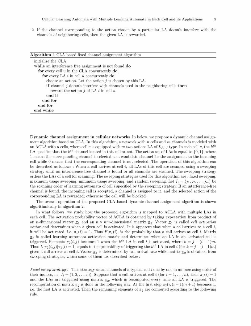
2. If the channel corresponding to the action chosen by a particular LA doesn’t interfere with thechannels of neighboring cells, then the given LA is rewarded.

Algorithm 1 CLA based fixed channel assignment algorithm

initialize the CLA.while an interference free assignment is not found do

for every cell u in the CLA concurrently dofor every LA i in cell u concurrently do

choose an action. Let the action j is chosen by this LA.if channel j doesn’t interfere with channels used in the neighboring cells then

reward the action j of LA i in cell u.end if

end forend for

end while

Dynamic channel assignment in cellular networks In below, we propose a dynamic channel assign-ment algorithm based on CLA. In this algorithm, a network with n cells and m channels is modeled withan ACLA with n cells, where cell v is equipped with m two-actions LA of LR−I type. In each cell v, the kth

LA specifies that the kth channel is used in this cell or not. The action set of LAs is equal to {0, 1}, where1 means the corresponding channel is selected as a candidate channel for the assignment to the incomingcall while 0 means that the corresponding channel is not selected. The operation of this algorithm canbe described as follows : When a call arrives at cell i, all LAs of this cell are scanned using a sweepingstrategy until an interference free channel is found or all channels are scanned. The sweeping strategyorders the LAs of a cell for scanning. The sweeping strategies used for this algorithm are : fixed sweeping,maximum usage sweeping, minimum usage sweeping, and random sweeping. Let Ii = (j1, j2, . . . , jm) bethe scanning order of learning automata of cell i specified by the sweeping strategy. If an interference-freechannel is found, the incoming call is accepted, a channel is assigned to it, and the selected action of thecorresponding LA is rewarded; otherwise the call will be blocked.

The overall operation of the proposed CLA based dynamic channel assignment algorithm is shownalgorithmically in algorithm 2.

In what follows, we study how the proposed algorithm is mapped to ACLA with multiple LAs ineach cell. The activation probability vector of ACLA is obtained by taking expectation from product ofan n-dimensional vector π1 and an n × nm-dimensional matrix π2. Vector π1 is called cell activationvector and determines when a given cell is activated. It is apparent that when a call arrives to a cell i,it will be activated, i.e. π1(i) = 1. Thus E[π1(i)] is the probability that a call arrives at cell i. Matrixπ2 is called learning automata activation matrix and determines when an LA in an activated cell istriggered. Elements π2(i, j) becomes 1 when the kth LA in cell i is activated, where k = j − (i − 1)m.Thus E[π2(i, j)|π1(i) = 1] equals to the probability of triggering the kth LA in cell i (for k = j− (i−1)m)given a call arrives at cell i. Vector π1 is determined by call arrival rate while matrix π2 is obtained fromsweeping strategies, which some of them are described below.

Fixed sweep strategy : This strategy scans channels of a typical cell i one by one in an increasing order oftheir indices, i.e. Ii = (1, 2, . . . , m). Suppose that a call arrives at cell i (for i = 1, . . . , n), then π1(i) = 1and the LAs are triggered using matrix π2, which is recomputed every time an LA is triggered. Therecomputation of matrix π2 is done in the following way. At the first step π2(i, (i− 1)m + 1) becomes 1,i.e. the first LA is activated. Then the remaining elements of π2 are computed according to the followingrule.


Algorithm 2 CLA based dynamic channel assignment algorithm

initialize the CLA.loop

for every cell u in the CLA concurrently doorder LAs using the given sweeping strategy and put in list Lu.wait for a call.set k ← 1; found← falsewhile k ≤ m and not found do

LA ALu(k) chooses one of its actions, where ALu(k) is the kth LA in list Lu.if selected action is 1 then

if selected channel doesn’t interfere with channels used in neighboring cells thenassign the channel and reward the selected action of ALu(k)

set found← trueend if

end ifSet k ← k + 1

end whileif not found then

block the incoming callend if

end forend loop

π2(i, j) =

⎧⎨⎩

1 if π1(i) = 1 and π2(i, j − 1) = 1

0 otherwise,(4)

for j = (i − 1)m + 2, . . . , im. In other words, in this strategy, LAs in cell i are triggered sequentially inincreasing order of their indices until a channel is found for the assignment.

Maximum usage strategy : In this strategy, the set of LAs in cell i are triggered in decreasing order oftheir usage of their corresponding channels until a non-interfering channel is found. If no channel can befound, then the incoming call will be blocked. In other words, in this strategy, LA Ak is triggered in thekth stage of the activation of cell i if ui

k is the kth largest element in usage vector ui = {ui1, u

i2, . . . , u

im},

where uik is the number of times that channel j is assigned to calls in cell i.

Minimum usage strategy : In this strategy, the set of LAs in cell i are triggered in increasing order oftheir usage of their corresponding channels until a non-interfering channel is found. If no channel can befound, then the incoming call will be blocked. In other words, in this strategy, LA Ak is triggered in thekth stage of the activation of cell i if ui

k is the kth largest element in usage vector ui = {ui1, u

i2, . . . , u

im},

where uik is the number of times that channel j is assigned to calls in cell i.

Random sweep strategy : In this strategy, the set of LAs in cell i are triggered in random order. Firsta sequence of indices are generated randomly and then the set of LAs are triggered according to thisgenerated order.

4.2 Cellular learning automata based evolutionary computing

Evolutionary algorithms (EAs) are a class of random search algorithms in which principles of naturalevolution are regarded as rules for optimization. They attempt to find the optimal solution to problemsby manipulating a population of candidate solutions. The population is evaluated and the best solutionsat each generation are selected to reproduce and mate to form the next generation. Over a number ofgenerations, good traits dominate the population, resulting in an increase in the quality of the solutions.


Cellular learning automata based evolutionary computing (CLA-EC), which is an application of syn-chronous CLA with multiple LAs in each cell is obtained by combining CLA and evolutionary computingmodels [24]. In CLA-EC, each genome in the population is assigned to one cell of CLA and each cell inCLA is equipped with a set of LAs, each of them corresponds to one gene in the genome. The populationis made from genomes of all cells. The operation of CLA-EC can be described as follows: At the firststep, all LAs in the CLA-EC choose their actions synchronously. The set of actions chosen by LA of acell determine the string genome for that cell. Based on a local rule, a vector of reinforcement signals isgenerated and given to the LAs residing in the cell. All LAs in the CLA-EC update their action probabil-ity vectors based on the received reinforcement signal using a learning algorithm. The process of actionselection and updating the internal structure of LAs is repeated until a predetermined criterion is met.

CLA-EC has been used in several applications such as function optimization, and data clustering tomention a few [24]. In what follows, we present an algorithm based on CLA-EC for function optimizationproblem. Assuming a binary finite search space, a function optimization problem can be described as theminimization of a real function f : {0, 1}m → R. In this algorithm, the chromosome is represented usinga binary string of m bits and then each cell of CLA-EC is equipped with m two actions LAs, each ofwhich is responsible for updating a gene. The actions set of all LAs corresponds to the set {0, 1}. Thenthe following steps are repeated until the termination criterion is met.

1. All LAs choose their actions synchronously.2. Concatenate the chosen actions of LAs in ech cell i and generate a new chromosome αi.3. The fitness of all chromosomes are computed. If the fitness of the new chromosome of a cell is better

than the previous one, it will be replaced.4. A set of Ns(i) neighboring cells of each cell i is selected.5. In the selected neighbors, the number of cells with the same value of genes are counted. Let Nij(k)

be the number of jth genes that have the same value of k at the selected neighboring cells of i. Thenthe reinforcement signal for jth LA of cell i is computed as

βij =

⎧⎨⎩

U [Nij(1)−Nij(0)] if αij = 0

U [Nij(0)−Nij(1)] if αij = 1,

(5)

where αij is the value of jth gene in the ith chromosome and U(.) is the step funtion.

The overall operation of the CLA-EC based optimization algorithm is shown algorithmically in algo-rithm 3.

Algorithm 3 CLA-EC based optimization algorithm

initialize the CLA.while not done do

for every cell i in the CLA concurrently dogenerate a new chromosome.evaluate the new chromosome.if fitness of new chromosome is better than the previous one then

replace the previous chromosome by the new one.end ifselect Ns(i) neighboring cellsgenerate the reinforcement signal for all LAs.update action probability vectors of all LAs.

end forend while


5 Computer Experiments

In this section, we give three sets of computer simulations for CLA with multiple LAs in each cell. The firsttwo experiments are the simulations of the proposed fixed and dynamic channel assignment algorithmsand the next one is the results of CLA-EC based function optimization algorithm.

5.1 Channel assignment in cellular networks

In order to show the effectiveness of the proposed CLA based channel assignment algorithms computersimulations are conducted. In these simulations, interference is shown by a constraint matrix C. Theelement c(u, v) of constraint matrix C, which represents the minimum gap among channels assigned tocells u and v, are defined on the basis of normalized distance of cells u and v, denoted by d(u, v). Inthe rest of this section, the simulation results of the proposed fixed and dynamic channel assignmentalgorithms are given.

Fixed channel assignment in cellular networks In this section, we give the results for the proposedfixed channel assignment algorithm for a simplified version of Philadelphia problem. The Philadelphiaproblem is a channel assignment problem based on a hypothetical, but realistic cellular mobile networkcovering the region around this city [25]. The cellular network of the Philadelphia problem is based on aregular grid with 21 cells shown in figure 3.

Fig. 3. The cellular network of the Philadelphia problem.

In the Philadelphia problem, the interference constraints between any pair of cells is represented byan integer, c(i, j), as defined below.

c(i, j) =

⎧⎨⎩

5 if i = j2 if 0 < d(i, j) ≤ 11 if 1 < d(i, j) ≤ 2

√3.

(6)

The demand vector of the Philadelphia problem is given in table 1.

Table 1. The demand vector for Philadelphia problem.

Cell 1 2 3 4 5 6 7 8 9 10 11 12 13 14 15 16 17 18 19 20 21

Demand 8 25 8 8 8 15 18 52 77 28 13 15 31 15 36 57 28 8 10 13 8

If we wanted to solve the original version of Philadelphia problem, we needed to have in each cellseveral LAs with large number of actions, which leads to slow rate of convergence of CLA to its compatibleconfiguration. To speed up the convergence of CLA, we have simplified the original version of Philadelphia


problem by simplifying the constraint matrix and the demand vector. To obtain our simplified version ofPhiladelphia problem we have changed the interference model and demand vector as explained below. Inthe simplified version of the problem, the interference c(i, j) is defined as follows.

c(i, j) =

⎧⎨⎩

2 if i = j1 if d(i, j) = 10 otherwise.

(7)

Note that c(i, j) will be zero if there is no interference between two cells i and j. Each cell and at mostits six neighboring cells constitute a cluster. The cells in this cluster define the neighboring cells in CLA.In the simplified version of the Philadelphia problem, we consider two demand vectors given in table 2.

Table 2. The demand vectors for modified version of Philadelphia problem.

Cell 1 2 3 4 5 6 7 8 9 10 11 12 13 14 15 16 17 18 19 20 21

Demand 1 1 1 1 1 1 1 1 1 1 1 1 1 1 1 1 1 1 1 1 1 1Demand 2 1 1 1 1 1 2 2 2 2 2 2 2 2 2 1 1 2 2 2 2 2

Figures 4 and 5 show the evolution of the interference in the cellular network with different set ofchannels during the the operation of the network. These figures show that 1) the interference is decreasingas time goes on, 2) the interference becomes zero when CLA converges, and 3) by increasing the numberof channels allocated to the network, the speed of convergence of CLA also increases.

Fig. 4. The interference for different channels for demand vector 1.

Dynamic channel assignment in cellular networks In this section, we present the simulationresults of the proposed CLA based dynamic channel assignment algorithm and compare it with tworelated dynamic channel assignment algorithms : channel segregation [21] and reinforcement learning[22] algorithms. For simulations, it is assumed that there are seven base stations, which are organized ina linear array, share 5 full duplex and interference free channels. In these simulations, the interferenceconstraints between any pair of cells represented by c(i, j) and defined as follows.


Fig. 5. The interference for different channels for demand vector 2.

c(i, j) =

⎧⎨⎩

1 if d(i, j) ≤ 2

0 otherwise.(8)

The elements in matrix C corresponding to pairs of non-interfering cells are defined to be zero. Weassume that the arrival of calls is Poisson process with rate λ and channel holding time of calls isexponentially distributed with mean μ = 1/3. We also assume that no handoff occurs during the channelholding time. The results of simulations reported in this section are obtained from 120, 000 secondssimulations. Figure 6 shows the average blocking probability of calls for the proposed algorithm andcompared with results obtained for channel segregation and reinforcement learning algorithms. Figure7 shows the average blocking probabilities for different strategies for a typical run. Figure 8 shows theevolution of the interference as the CLA operates. Figure 7 and 8 show that the blocking probability andinterference decreases as the learning proceeds. That is, the CLA segregates channels among the cells ofthe network.

Figures 9 and 10 show the probability of assigning different channels to different cells for differentsweeping strategies for a typical simulation. These figures show that the proposed algorithm can segregatechannels among different cells of network.

The simulation results presented for fixed and dynamic channel assignment algorithms show thatthe CLA based algorithms may converge to local optima as shown theoritically in [10–12]. This maydue to access to the limited information in each cell. In order to alleviate this problem, we can allowadditional information regarding channels in the network to be gathered and used by each cell in orderto allocate channels. The additional information help cellular learning automata to find an assignmentwhich results in lower blocking probability for the network. In [26], a CLA based dynamic channelassignment algorithm is given that allows additional information to be exchanged among neighboringcells.The simulation results show that the exchange of additional information among neighboring celldecreases the blocking probability of calls.

5.2 Function optimization

This section presents the experimental results for two function optimization problems and then comparethese results with results obtained using Simple Genetic Algorithm (SGA) [27], Population based Incre-mental Learning (PBIL) [28] and Compact Genetic Algorithm (cGA) [29] in terms of solution quality,and the number of function evaluations taken by the algorithm to converge completely for a given pop-ulation size. A CLA completely converges when all learning automata residing in all cells converge. The


Fig. 6. Average blocking probability.

Fig. 7. Evolution of blocking probability for a typical run.


Fig. 8. Evolution of interference among channels assigned to neighboring cells.

Fig. 9. Probability of assigning different channels to different cells for fixed sweep strategy.


Fig. 10. Probability of assigning different channels to different cells for maximum usage strategy.

algorithm terminates when all learning automata converge. Each quantity of the reported results is theaverage taken over 20 runs. The algorithm uses one-dimensional CLA uses LR−I learning automata ineach cell and neighborhood vector N = {−1, 0, +1}. The CLA based algorithm is tested on two differentstandard function minimization problems. These functions that are given below are borrowed from [30].

Second De Jongs function

F2(x1, x2) = 100(x21 − x2)2 + (1− x1)2 −2.048 ≤ x1, x2 ≤ 2.048 (9)

Forth De Jongs function

F4(x1, x2) =∑30

i=1 i× x4i + N(0, 1) −1.28 ≤ xi ≤ 1.28 (10)

In order to study the speed of the convergence of CLA-EC, the best, the worst, the mean and thestandard deviation of fitness of all cells for each of the function optimization problem are reported.Figures 11 and 12 show the result of simulations for F2 and F4. Simulation results indicate that CLA-ECconverges to near of an optimal solution. For these experiments Ns(i) is set to 2 and learning parametersof all LAs are set to 0.01.

The size of CLA-EC (population size) is another important parameter, which affects the performanceof CLA-EC. Figures 13 and 14 show the effect of the size of CLA-EC on speed of convergence of CLA-EC.Each point in these figures shows the best fitness obtained at one iteration. For these experiments Ns(i)is set to 2 and learning parameters of all LAs are set to 0.01. The results of computer experiments showthat as the size of CLA-EC increases the speed of convergence increases. However, it is observed that forsome experiments, there exists a value if the size of the CLA-EC increases beyond that, no increase inthe performance occurs .

Figures 15 and 16 compare the performance of CLA-EC with SGA [11], cGA [13], and PBIL [2]. TheSGA uses two-tournament selection without replacement and uniform crossover with exchange probability0.5. Mutation is not used and crossover is applied with probability one. The PBIL uses learning rate 0.01and the number of selection genomes is half of the population size. The parameters of cGA is the sameas the parameters used in [13]. Convergence is considered as the termination condition for all algorithms.For these experiments Ns(i) is set to 2 and learning parameters of all LAs are set to 0.01. Results showthe superiority of the CLA-based algorithm over the SGA, PBIL and cGA.


Fig. 11. Evolution of five cells CLA-EC for F2.

Fig. 12. Evolution of five cells CLA-EC for F4.


Fig. 13. Effects of population size on the volution of five cells CLA-EC for F2.

Fig. 14. Effects of population size on the volution of five cells CLA-EC for F4.


Fig. 15. Comparison of CLA-EC with some other algorithms for F2.

Fig. 16. Comparison of CLA-EC with some other algorithms for F4.


6 Conclusions

In this paper, the cellular learning automata with multiple learning automata in each cell was introducedand its steady state behavior was studied. It is shown that for commutative rules, this cellular learningautomata converges to a stable configuration for which the average reward for the CLA is maximum.Then two applications of the proposed model to channel assignment in cellular mobile networks andfunction optimization are given. For both applications, computer simulations shown that the cellularlearning automata based solutions produce better results. The numerical results also confirm the theory.New research on CLA can be pursuit on several directions: 1) searching for new applications; at presenttime, applications of CLA to the sensor networks and ad hoc networks are being undertaken, 2) to studythe behavior of CLA for different local rules, and 3) development of extended versions of CLA such asirregular CLA, dynamic CLA, and associative CLA.

References

1. N. H. Packard and S. Wolfram, “Two-Dimensional Cellular Automata,” Journal of Statistical Physics, vol. 38,pp. 901–946, 1985.

2. E. Fredkin, “Digital Machine: A Informational Process Based on Reversible Cellular Automata,” Physica D,vol. 45, pp. 254–270, 1990.

3. J. Kari, “Reversability of 2D Cellular Automata is Undecidable,” Physica D, vol. 45, pp. 379–385, 1990.4. G. I. Papadimitriou, M. S. Obaidat, and A. S. Pomportsis, “On the Use of Learning Automata in the Control

of Broadcast Networks: A Methodology,” IEEE Transactions on Systems, Man, and Cybernetics–Part B:Cybernetics, vol. 32, pp. 781–790, Dec. 2002.

5. S. Misra, K. I. Abraham, M. S. Obaidat, and P. V. Krishna, “ LAID: A Learning Automata-Based Schemefor Intrusion Detection in Wireless Sensor Networks,” Security and Communication Networks, vol. 2, no. 2,pp. 105–115, 2009.

6. E. Fayyoumi and B. J. Oommen, “Achieving Micro-Aggregation for Secure Statistical Databases Using FixedStructure Partitioning-Based Learning Automata,” IEEE Transactions on Systems, Man, and Cybernetics–Part B: Cybernetics, vol. 39, pp. 1192–1205, Oct. 2009.

7. H. Beigy and M. R. Meybodi, “Utilizing Distributed Learning Automata to Solve Stochastic Shortest PathProblems,” International Journal of Uncertainty, Fuzziness and Knowledge-Based Systems, vol. 14, pp. 591–615, Oct. 2006.

8. S. Misra and B. J. Oommen, “Using Pursuit Automata for Estimating Stable Shortest Paths in StochasticNetwork Environments,” International Journal of Communication Systems, vol. 22, pp. 441–468, 2009.

9. M. R. Meybodi, H. Beigy, and M. Taherkhani, “Cellular Learning Automata and its Applications,” SharifJournal of Science and Technology, vol. 19, no. 25, pp. 54–77, 2003.

10. H. Beigy and M. R. Meybodi, “Asynchronous Cellular Learning Automata,” Automatica, vol. 44, pp. 1350–1357, May 2008.

11. M. R. Meybodi and H. Beigy, “Open Synchronous Cellular Learning Automata,” Journal of Advances inComplex Systems, vol. 10, pp. 527–556, Sept. 2007.

12. M. R. Meybodi and H. Beigy, “A Mathematical Framework for Cellular Learning Automata,” Journal ofAdvances in Complex Systems, vol. 7, pp. 295–320, Sept. 2004.

13. M. R. Meybodi and M. R. Kharazmi, “Application of Cellular Learning Automata to Image Processing,”Journal of Amirkabir, vol. 14, no. 56A, pp. 1101–1126, 2004.

14. M. R. Meybodi and M. Taherkhani, “Application of Cellular Learning Automata in Modeling of Rumor Dif-fusion,” in Proceedings of 9th Conference on Electrical Engineering, Power and Water Institute of Technology,Tehran, Iran, pp. 102–110, May 2001.

15. M. R. Meybodi and M. R. Khojasteh, “Application of Cellular Learning Automata in Modelling of Com-merce Networks,” in Proceedings of 6th Annual International Computer Society of Iran Computer ConferenceCSICC-2001, Isfehan, Iran, pp. 284–295, Feb. 2001.

16. H. Beigy and M. R. Meybodi, A Self-Organizing Channel Assignment Algorithm: A Cellular Learning Au-tomata Approach, vol. 2690 of Springer-Verlag Lecture Notes in Computer Science, pp. 119–126. Springer-Verlag, 2003.

17. M. Esnaashari and M. R. Meybodi, “A Cellular Learning Automata Based Clustering Algorithm for WirelessSensor Networks,” Sensor Letters, vol. 6, no. 5, pp. 723–735, 2008.

18. K. S. Narendra and A. M. Annaswarmy, Stable Adaptive Systems. New York: Printice-Hall International Inc.,1989.


19. I. Katzela and M. Naghshineh, “Channel Assignment Schemes for Cellular Mobile Telecommunication Sys-tems: A Comprehensive Survey,” IEEE Personal Communications, vol. 3, pp. 10–31, June 1996.

20. W. K. Hale, “Frequence Assignment: Theory and Applications,” Proceedings of IEEE, vol. 68, pp. 1497–1514,Dec. 1980.

21. Y. Furuya and Y. Akaiwa, “Channel Segregation– A Distributed Channel Allocation Scheme for MobileCommunication Systems,” IEICE Trans, vol. 74, no. 6, pp. 1531–1537, 1991.

22. S. Singh and D. P. Bertsekas, “Reinforcement Learning for Dynamic Channel Allocation in Cellular Tele-phone Systems,” in Advances in Neural Information Processing Systems: Proceedings of the 1996 Conference,Cambridge, MA. MIT Press, 1997.

23. J. Li, N. B. Shroff, and E. K. P. Chong, “Channel Carrying: A Novel Handoff Scheme for Mobile CellularNetworks,” IEEE/ACM Transactions on Networking, vol. 4, pp. 35–50, Feb. 1999.

24. R. Rastegar, M. R. Meybodi, and A. Hariri, “A New Fine-Grained Evolutionary Algorithm Based on CellularLearning Automata,” International Journal of Hybrid Intelligent Systems, vol. 2, no. 2, pp. 82–98, 2006.

25. J. C. M. Janssen and K. Kilakos, “An Optimal Solution to the Philadelphia Channel Assignment Problem,”IEEE Transactions on Vehicular Technology, vol. 48, pp. 1012–1014, May 1999.

26. H. Beigy and M. R. Meybodi, “Cellular Learning Automata Based Dynamic Channel Assignment Algorithms,”International Journal of Computational Intelligence and Applications, Accepted for Publication.

27. D. E. Goldberg, Genetic Algorithms in Search, Optimization and Machine Learning. Addison-Wesley, 1987.28. S. Baluja and R. Caruana, “Removing The Genetics from The Standard Genetic Algorithm,” in Proceedings

of ICML’95, Palo Alto, CA, pp. 38–46, 1995.29. G. R. Harik, F. G. Lobo, and D. E. Goldberg, “The Compact Genetic Algorithm,” IEEE Transaction on

Evolutionary Computing, vol. 3, no. 4, pp. 287–297, 1999.30. K. A. D. Jong, The Analysis of the Behavior of a Class of Genetic Adaptive Systems. PhD thesis, University

of Michigan, Ann Arbor, 1975.

cellular learning automata with multiple learning automata...

Documents