Cellular Automata• Grid of cells, connected to neighbors

– Spatial organization. Typically 1 or 2 dimensional• Time and space are both discrete• Each cell has a state

– Cell’s state at t+1 depends only on states of its neighbors anditself at t. Behavior is determined locally

One-dimensional Cellular Automata

Transition Rules

Tim

e

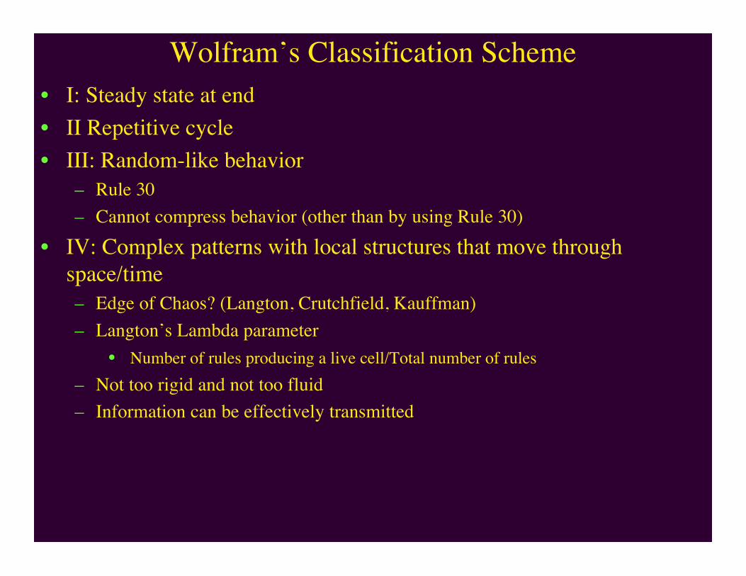
Wolfram’s Classification Scheme• I: Steady state at end• II Repetitive cycle• III: Random-like behavior

– Rule 30– Cannot compress behavior (other than by using Rule 30)

• IV: Complex patterns with local structures that move throughspace/time– Edge of Chaos? (Langton, Crutchfield, Kauffman)– Langton’s Lambda parameter

• Number of rules producing a live cell/Total number of rules– Not too rigid and not too fluid– Information can be effectively transmitted

Type 1: Steady-state Patterns

Type 2: Repetitive Cycles

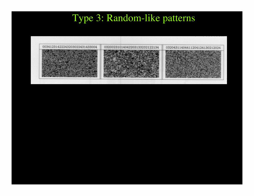
Type 3: Random-like patterns

Type 4: Local Structures that Move

Langton’s Lambda Parameter

l=10/32, Type II l=12/32, Type IV

l=14/32, Type III

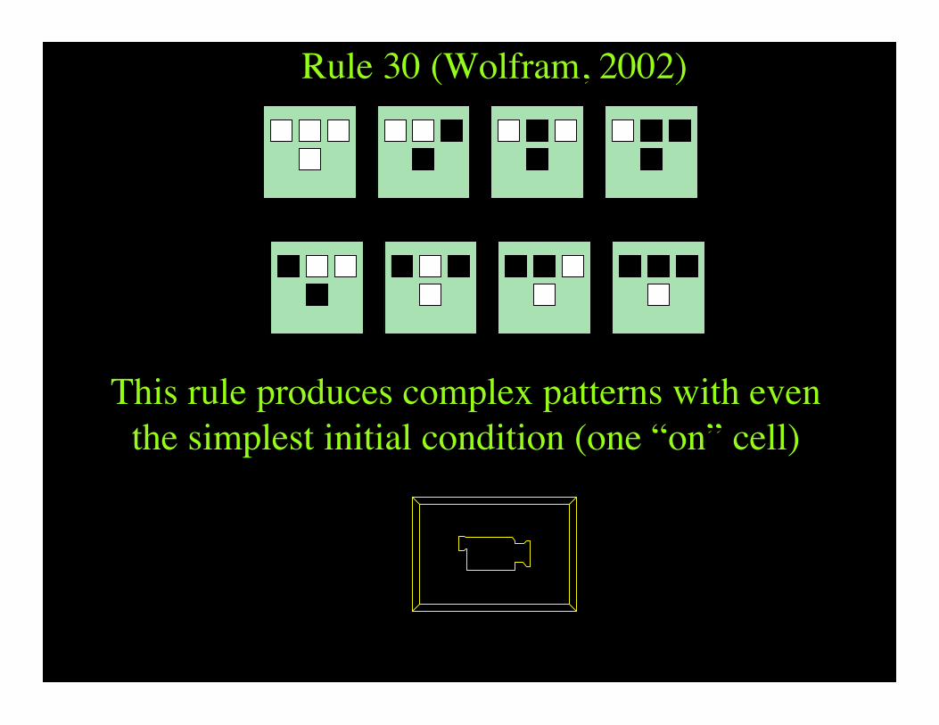
Rule 30 (Wolfram, 2002)

This rule produces complex patterns with eventhe simplest initial condition (one “on” cell)

Sensitivity to initial conditions

Changing one cell in initial seed pattern causes acascade of changes

Rule 30

Rule 22

Cellular Automata Terminology• Cell-space: define a lattice structure with maximum

extent of n columns and m rows

• Moore neighborhood: N, S, E, W and diagonal neighbors

• Von Neumann: only N, S, E, W cells

†

L = (i, j) | i, j Œ N,0 £ i < n,0 £ j < m{ }

†

Ni, j = k,l( ) Œ L k - i £1and l - j £1{ }

†

Ni, j = k,l( ) Œ L k - i + l - j £1{ }

n

m

Cellular Automata Terminology• Totalistic rules

– the state of the next state cell is only dependent upon the sum of thestates of the neighbor cells

• Reversible rules– No application of the rules loses any information– For every obtainable state there is only state that can produce it– Atypical, because these do not incorporate cell interactions– Sometimes applied in modeling physical systems (e.g. billiard balls)

Cellular Automata Broadened• Mobile automata

– A single active cell, which updates its position and state

• Turing Machines– The active cell has a state, and states determine which transition rule is

applied

• Substitution Systems– On each iteration, each cells is replaced with a set of cells

• Tag systems– Remove cells from left, and add to the right depending on removed cells

• Continuous state systems– On each iteration, each cells is replaced with a set of cells

• Asynchronously updating systems

Mobile automata

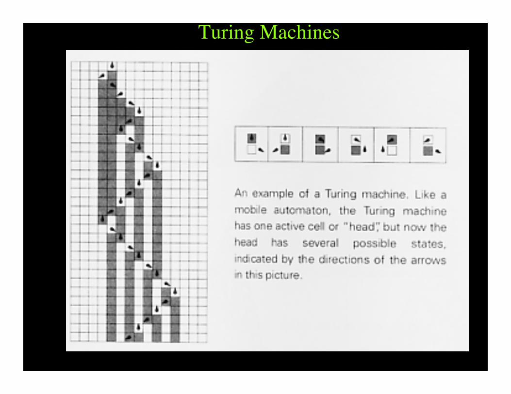
Turing Machines

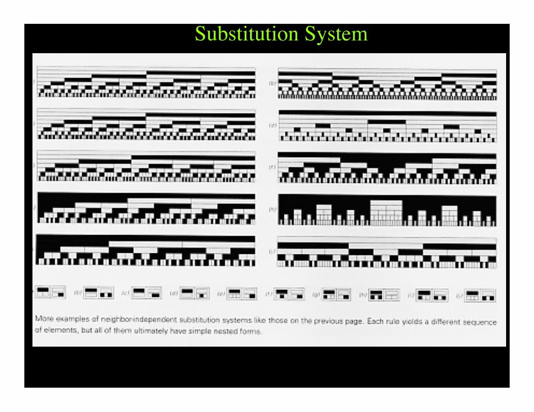
Substitution System

Cantor’s Set

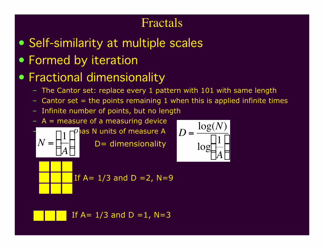
Fractals• Self-similarity at multiple scales• Formed by iteration• Fractional dimensionality

– The Cantor set: replace every 1 pattern with 101 with same length– Cantor set = the points remaining 1 when this is applied infinite times– Infinite number of points, but no length– A = measure of a measuring device– An object has N units of measure A

†

N =1A

Ê

Ë Á

ˆ

¯ ˜

D

D= dimensionality

†

D =log(N)

log 1A

Ê

Ë Á

ˆ

¯ ˜

If A= 1/3 and D =2, N=9

If A= 1/3 and D =1, N=3

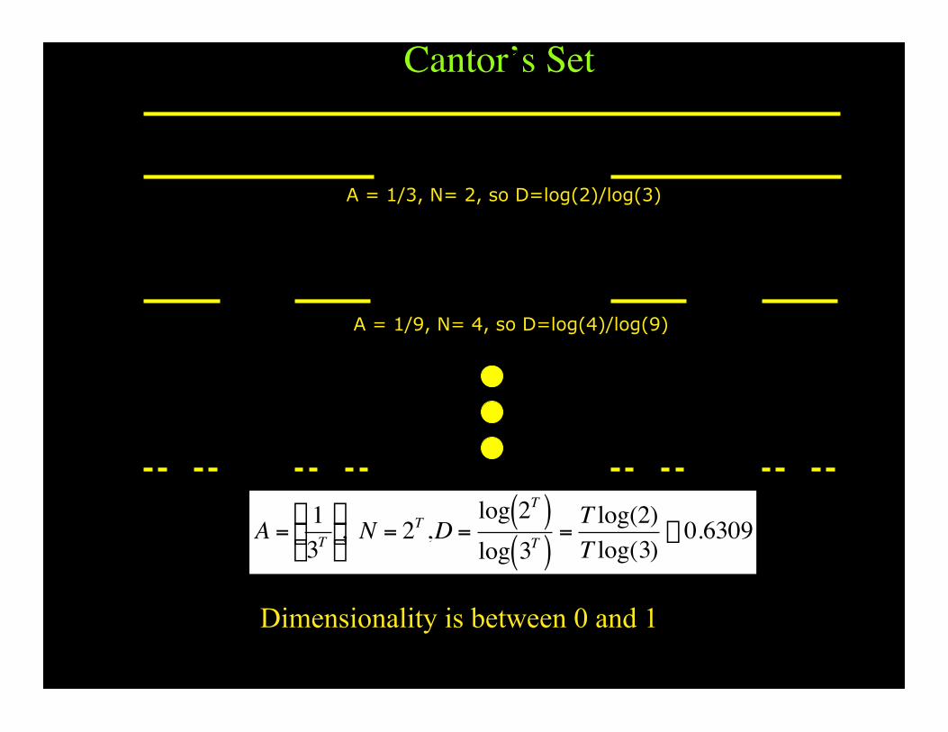
Cantor’s Set

A = 1/3, N= 2, so D=log(2)/log(3)

A = 1/9, N= 4, so D=log(4)/log(9)

†

A =13T

Ê

Ë Á

ˆ

¯ ˜ , N = 2T ,D =

log 2T( )log 3T( )

=T log(2)T log(3)

@ 0.6309

Dimensionality is between 0 and 1

Hilbert’s Space Filling Curve• Dimensionality = 2 as iterations go to infinity even

though it is a single line• Fractals: measure of object increases as the measuring

device decreases

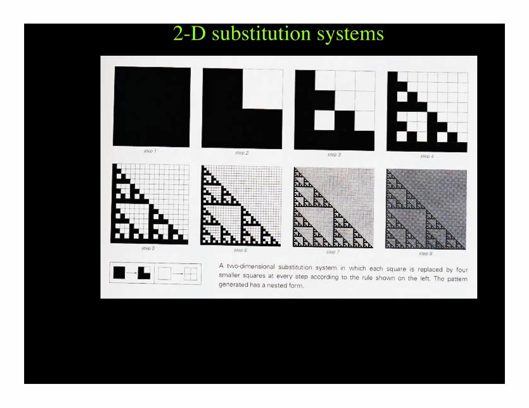
2-D substitution systems

L-Systems for plant growthSubstitution system

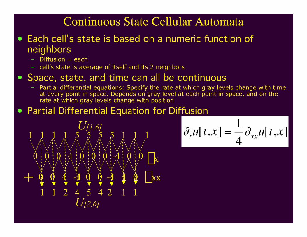
Continuous State Cellular Automata• Each cell’s state is based on a numeric function of

neighbors– Diffusion = each– cell’s state is average of itself and its 2 neighbors

• Space, state, and time can all be continuous– Partial differential equations: Specify the rate at which gray levels change with time

at every point in space. Depends on gray level at each point in space, and on therate at which gray levels change with position

• Partial Differential Equation for Diffusion

†

∂tu[t,x] =14

∂xxu[t,x]1 1 1 1 5 5 5 5 1 1 1

0 0 0 4 0 0 0 -4 0 0

0 0 4 -4 0 0 -4 4 00 0 1 -1 0 0 -1 1 0

1 1 2 4 5 4 2 1 1

dx

dxx

U[1,6]

U[2,6]

+

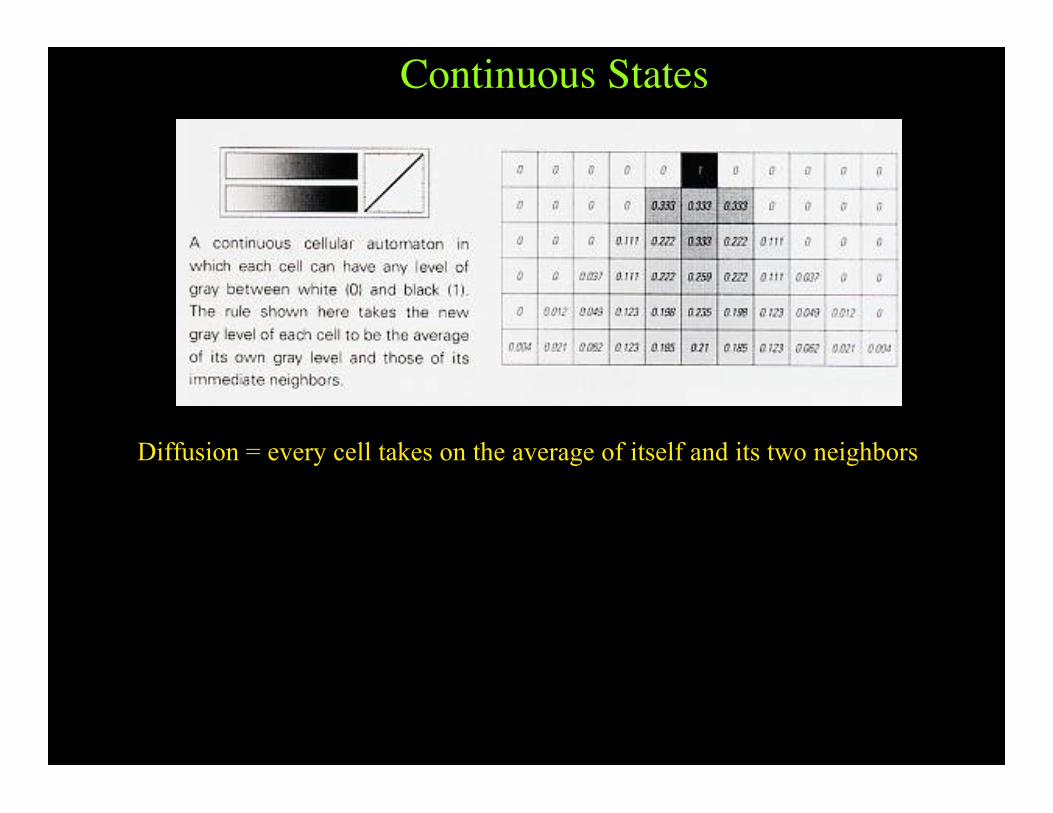
Continuous States

Diffusion = every cell takes on the average of itself and its two neighbors

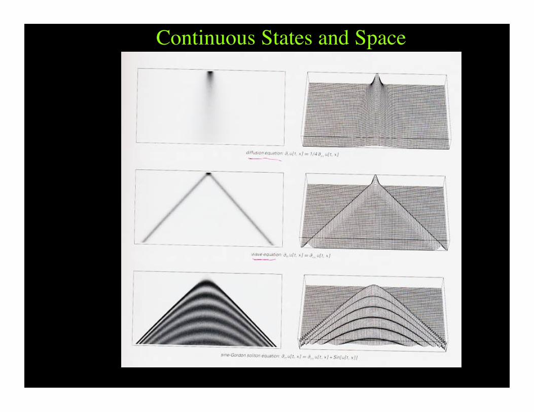
Continuous States and Space

Discrete transitions from continuous systems

Order from random configurations

Apparent randomness from orderly configurations

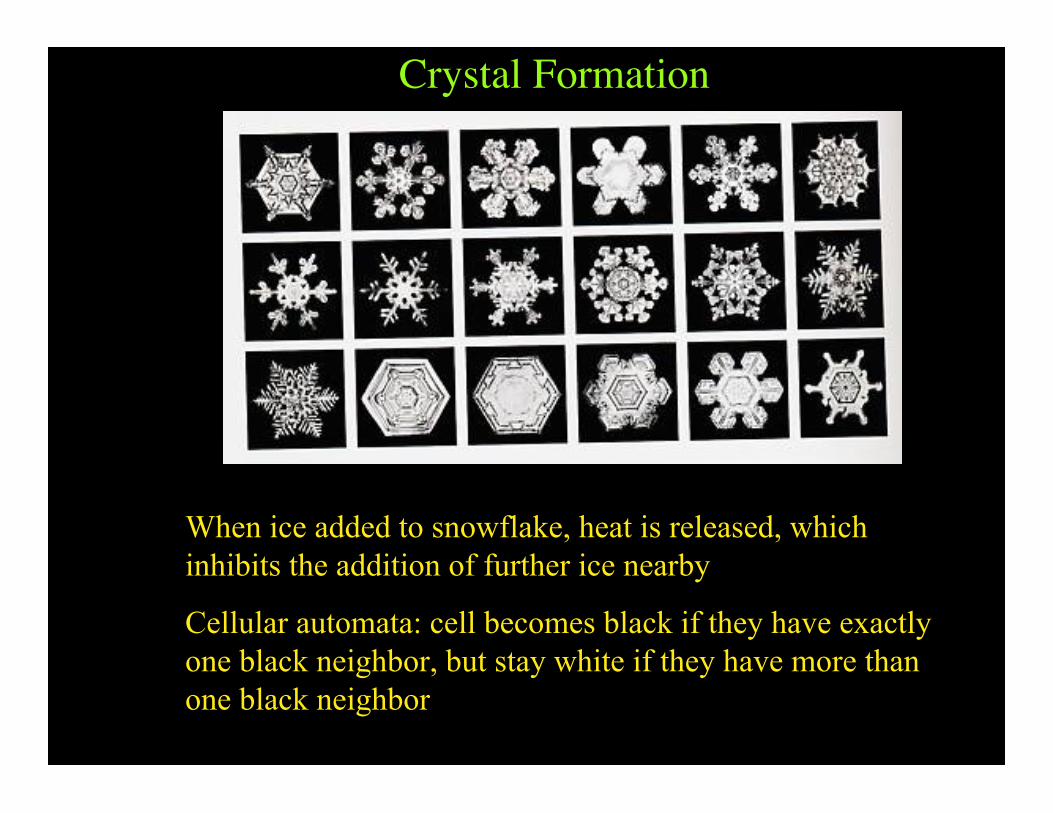
Crystal Formation

When ice added to snowflake, heat is released, whichinhibits the addition of further ice nearby

Cellular automata: cell becomes black if they have exactlyone black neighbor, but stay white if they have more thanone black neighbor

Crystal Formation

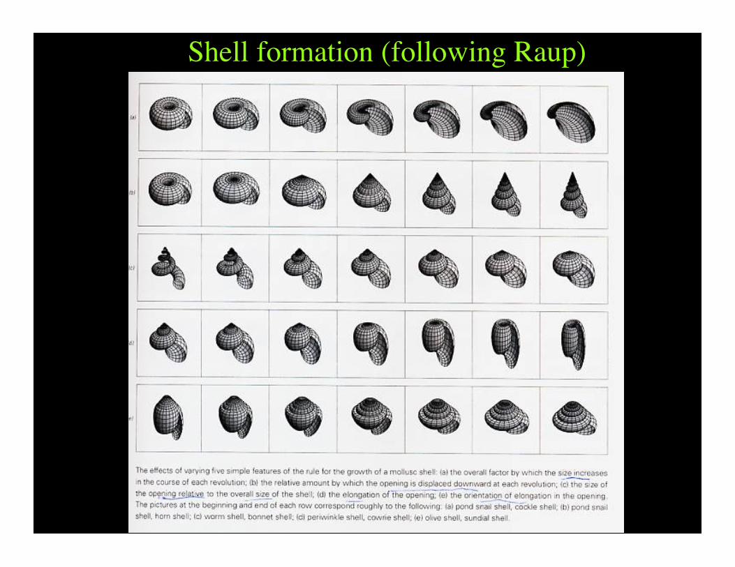
Shell formation (following Raup)

Model-world comparison

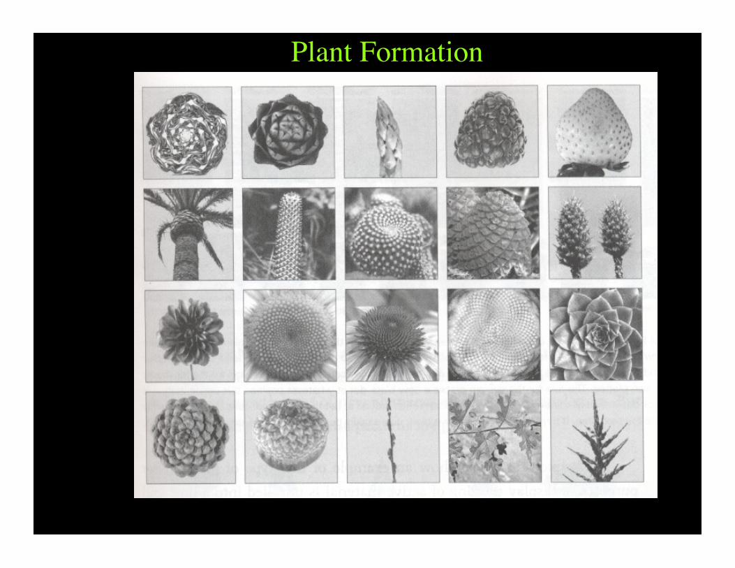
Plant Formation

Pine Cone Spirals

The numbers of clockwise and counter-clockwisespirals are successive numbers in the Fibonaccisequence: 1 1 2 3 5 8 13 21 34 55

The angle between successive leaves on the pinecone is 137.5 degrees

Golden Mean

A

C=1

A C-A

C

A=

A

C - A

C2-AC=A2

A2+A-1=0

The Golden Section

A

C=1

C-A

C2-AC=A2

A2+A-1=0

C

A=

A

C - A

Find the A such that

1

f

Golden Rectangle

The Golden Section

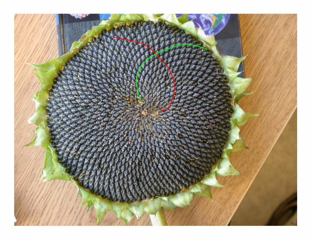
The angle between successive sunflower seeds is thegolden section of a circle

The ratio of successive numbers of a fibonacci sequenceapproximate f

f=.6180… 3/5=.6 8/13=.615 34/55=.6182

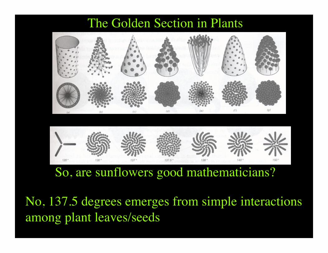
The Golden Section in Plants

So, are sunflowers good mathematicians?

No, 137.5 degrees emerges from simple interactionsamong plant leaves/seeds

Sunflower Seed Interactions

1

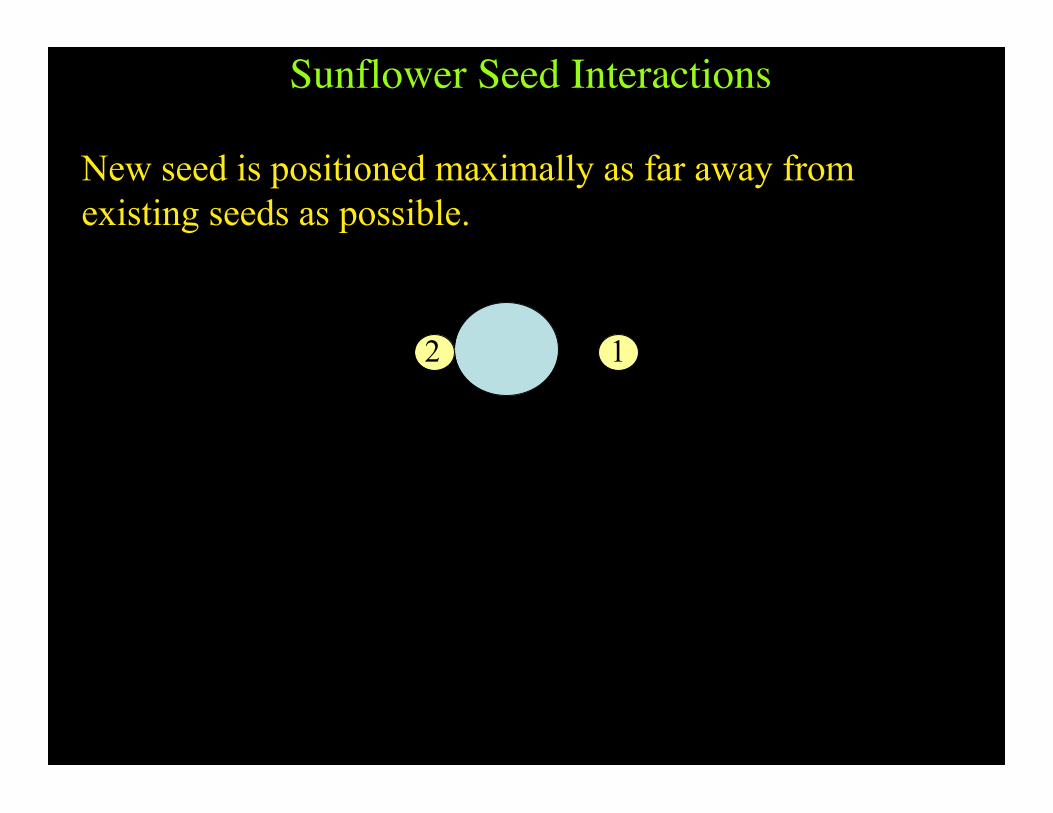
Sunflower Seed Interactions

12

New seed is positioned maximally as far away fromexisting seeds as possible.

Sunflower Seed Interactions

12

3

Seeds 1 and 2 both push Seed 3 away, but Seed 2 pushes morebecause it is closer to Seed 3.

Find location on circle for seed that minimizes the sum of the“push” exerted by other seeds, where push is an inverse squarefunction of distance

Sunflower Seed Interactions

12

3

4

≈137.5o

A simple model based on these interactions canprovide an account of many plant forms that arefound by varying only a few parameters.

Goodwin - evolutionary pressures as overrated?

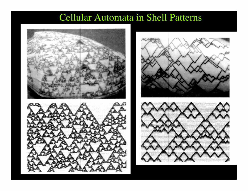
Cellular Automata in Shell Patterns

Pattern Formation

Pattern Formation (Morphogenesis)• Spots and Stripe formation• Activator-inhibitor systems

– Cells activate and inhibit neighboring cells– Close neighbors activate each other– Further neighbors inhibit each other– Mexican hat function in vision

Distance from cell

Infl

uenc

e on

cel

l

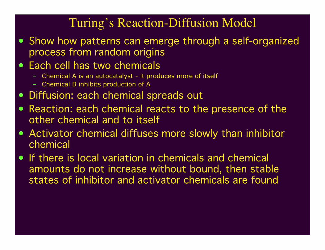
Turing’s Reaction-Diffusion Model• Show how patterns can emerge through a self-organized

process from random origins• Each cell has two chemicals

– Chemical A is an autocatalyst - it produces more of itself– Chemical B inhibits production of A

• Diffusion: each chemical spreads out• Reaction: each chemical reacts to the presence of the

other chemical and to itself• Activator chemical diffuses more slowly than inhibitor

chemical• If there is local variation in chemicals and chemical

amounts do not increase without bound, then stablestates of inhibitor and activator chemicals are found

Turing’s (1952) Reaction-Diffusion Model

DiffusionReaction

reaction diffusionion

A

B

-+

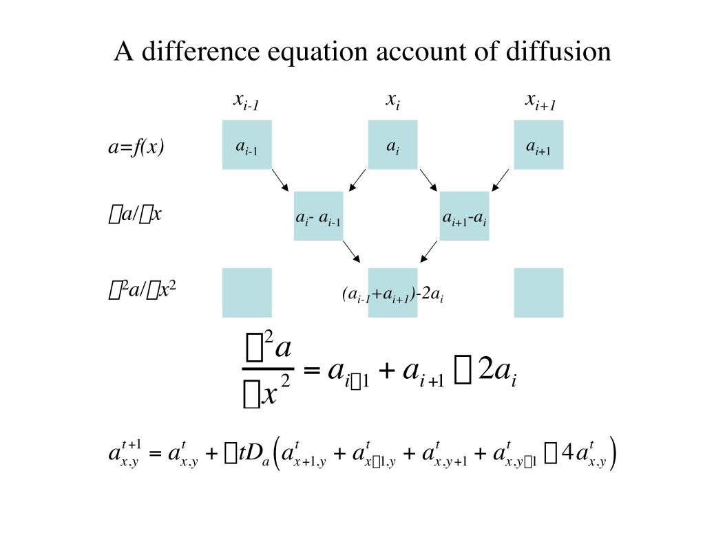
A difference equation account of diffusion

a=f(x) ai-1 ai ai+1

xi xi+1xi-1

(ai-1+ai+1)-2ai

†

D2aDx 2 = ai-1 + ai +1 - 2ai

ai- ai-1 ai+1-aiDa/Dx

D2a/Dx2

†

ax,yt +1 = ax,y

t + DtDa ax +1,yt + ax-1,y

t + ax,y +1t + ax,y-1

t - 4ax,yt( )

Pattern Formation with activator-inhibitor system

Stripe formation

Greater diffusion in one direction than the other

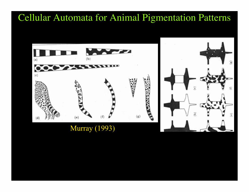
Cellular Automata for Animal Pigmentation Patterns

Murray (1993)

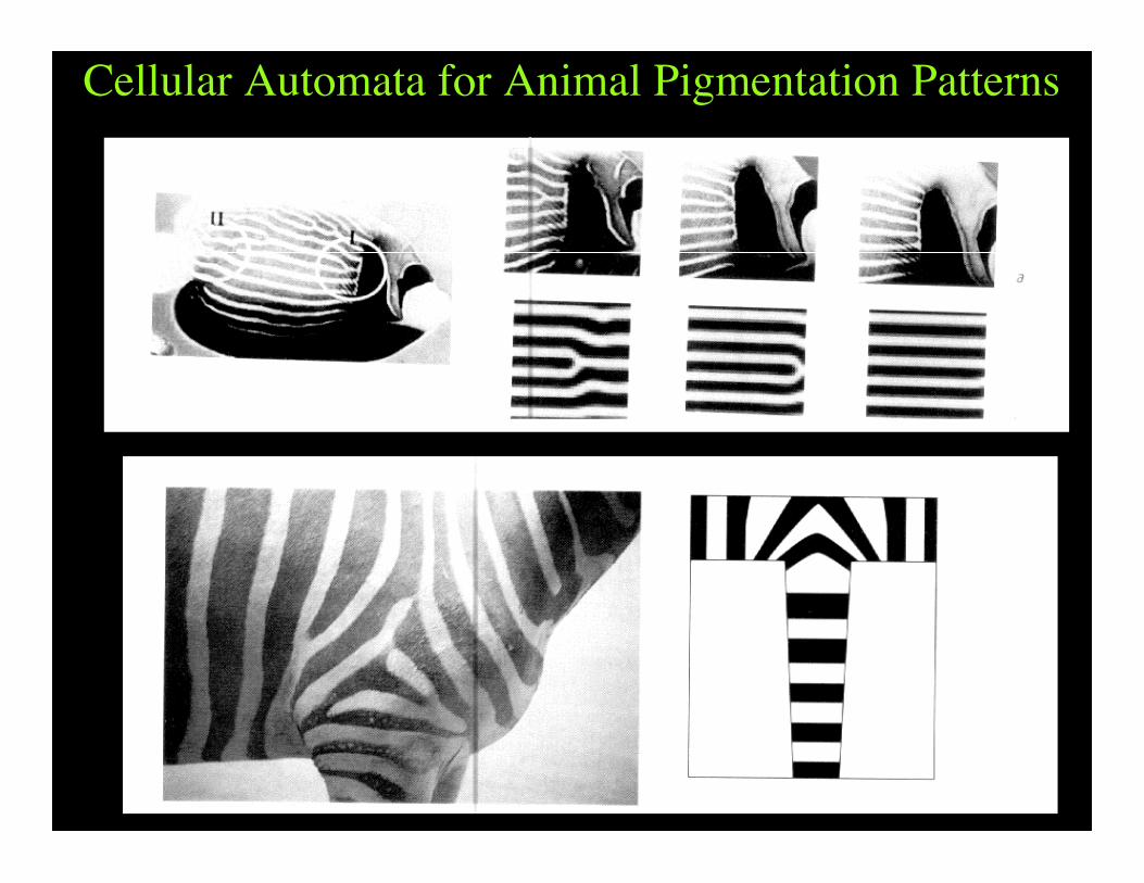
Cellular Automata for Animal Pigmentation Patterns

Diffusion Limited Aggregation for Population Growth