Page | 1 

CEE6400 Physical Hydrology Homework 6. Terrain Analysis and TOPMODEL Date: 10/23/13 Due: 11/4/13

LearningObjectives. Be able to use ArcGIS and TauDEM tools to derive hydrologically useful information from Digital 

Elevation Models (DEMs)  

Be able to describe the topographic wetness index used in TOPMODEL. (Rainfall Runoff 

Processes workbook chapter 6) 

Be able to use TOPMODEL principles to calculate soil moisture deficit and saturated areas as a 

function of wetness index and use this information in the calculation of runoff. (Rainfall Runoff 

Processes workbook chapter 6) 

Assignment1. Work through the material in chapter 6 of the online Rainfall Runoff Processes module at 

http://www.engineering.usu.edu/dtarb/rrp.html and do the quiz at the end.   2. Do the TauDEM watershed delineation exercise below. 3. Do the Logan River Hydrologic Annual Water Balance and Runoff Ratio exercise below. 4. Do the Spawn Creek TOPMODEL exercise below 

ComputerSetupDownload and install TauDEM following the instructions at 

http://hydrology.usu.edu/taudem/taudem5/downloads.html.  You will need administrator rights on the 

computer to do the installation.  TauDEM is already installed in the ENGR PC lab (ENGR 302) if you do 

your work there. 

2.TauDEMwatersheddelineationexerciseTauDEM (Terrain Analysis Using Digital Elevation Models) is a set of Digital Elevation Model (DEM) tools 

for the extraction and analysis of hydrologic information from topography as represented by a DEM.  

This is software developed at Utah State University (USU) for hydrologic digital elevation model analysis 

and watershed delineation and may be obtained from http://hydrology.usu.edu/taudem/taudem5/. 

The purpose of this exercise is to introduce Hydrologic Terrain Analysis in ArcGIS using the TauDEM 

toolbox and to guide you through the initial steps of installing TauDEM loading data and running some 

of the more important functions required to delineate a stream network and watershed.  This is a 

simplified version of tutorials given in the TauDEM documentation.  Refer to the TauDEM 

documentation if you want to learn about other TauDEM functions 

(http://hydrology.usu.edu/taudem/taudem5/documentation.html).    

In this exercise, you will perform the following tasks: - Basic Grid Analysis using TauDEM functions   

- Pit Remove 

- D8 Flow Directions 

Page | 2 

- D8 Contributing Area 

- Stream Network Analysis using TauDEM functions 

- Stream Definition by threshold 

- Stream Reach and Watershed 

 

The Logan River watershed draining to USGS streamflow gauge 10109000 located just east of Logan, 

Utah is used as an example.   

BasicGridAnalysisusingTauDEMfunctionsIn this section we illustrate the TauDEM basic grid analysis functions.   

 

1. Download the Logan River Exercise data zip file from 

http://www.neng.usu.edu/cee/faculty/dtarb/cee6400/Logan.zip.  Extract all files from the zip file.  

Open ArcMap and add the digital elevation model (DEM) grid file logan.tif into ArcMap. 

This digital elevation model (DEM) data was obtained from the National Elevation Dataset available from 

the national map (http://viewer.nationalmap.gov/viewer/), then projected and converted to the TIFF 

format required by TauDEM.  (To learn about georeferencing and projections in GIS see 

http://resources.arcgis.com/en/help/getting‐started/articles/026n0000000s000000.htm and 

http://resources.arcgis.com/en/help/main/10.1/index.html#//003r00000001000000. To learn how to 

convert files to TIFF format see 

http://hydrology.usu.edu/taudem/taudem5.0/TauDEM5GettingStartedGuide.pdf).   

In the below I have used symbology to select a different color scheme. 

 

Page | 3 

The first TauDEM function used is Pit Remove.  Pits are grid cells surrounded by higher terrain that do 

not drain.  Pit Remove creates a hydrologically correct DEM by raising the elevation of pits to the point 

where they overflow their confining pour point and can drain to the edge of the domain.  PitRemove is 

located in the TauDEM Tools Basic Grid Analysis group illustrated above.  If you do not find this in 

ArcMap, and TauDEM has been installed, you may need to add the TauDEM toolset to your document 

1. If the ArcToolbox Window is not open, click on the Toolbox icon   in the Standard 

Toolbar 

2. Right click on ArcToolbox at the top of the toolbox window. Select Add Toolbox... . 

3. Browse to the TauDEM install directory (usually C:\Program Files\TauDEM\ 

TauDEM5Arc\ or C:\Program Files (x86)\TauDEM\TauDEM5Arc\). 

4. Click on the TauDEM_Tools.tbx file, and click Open. 

5. If you wish right click on the ArcToolbox at the top and save settings to default so as not 

to have to do this again 

 

2. Open (by double clicking) the TauDEM Pit Remove Tool.  Select logan.tif for the Input Elevation 

Grid.  Note that the Output Pit Removed Elevation Grid is automatically filled with loganfel.tif 

following the file naming convention.  You may adjust or leave the number of processes at 8.  

  

The parallel approach used by TauDEM is illustrated below.   

 The domain is subdivided into row oriented partitions that are each processed independently by 

separate processes.  When the algorithms reach a point where they can proceed no further within the 

partitions there is a swap step that exchanges information along the boundaries.  The algorithms then 

proceed working within the partitions using new boundary information.  This process is iterated until 

Page | 4 

completion.  The strategies for sharing information across boundaries and iterating are specific to each 

algorithm. 

 

The number of processes does not have to be the same as the number of processors on your computer, 

although generally should be the same order of magnitude.  The operating system (and MPICH2) takes 

care of time sharing between processes, so in cases where some processes are likely to be waiting for 

other processes to complete there may be a benefit in selecting more processes than physical 

processors on the computer.  However then message passing across the borders is increased.  For large 

datasets, some experimentation as to the number of processes that works best (fastest) is suggested.  

For this exercise the functions run quickly and the number of processes does not matter too much.   

 

3. Click OK on the Pit Remove tool to run the Pit Remove function.  The output dialog reports run 

statistics that include timing, as well as any error or warning messages. 

 Clicking OK to run each tool will be implied from here on if not stated. 

 

Page | 5 

The result is a new grid layer loganfel.tif that has been added to the ArcMap Document.   

  

4. The next function to run is D8 Flow Direction with inputs as follows.   

  

This takes as input the hydrologically correct elevation grid and outputs D8 flow direction and slope for 

each grid cell.  The resulting D8 flow direction grid (name has suffix p) is illustrated.  This is an encoding 

of the direction of steepest descent from each grid cell using the numbers 1 to 8 (counter clockwise 

from east).  This is a simple model for the direction of water flow over the terrain.   

 

Page | 6 

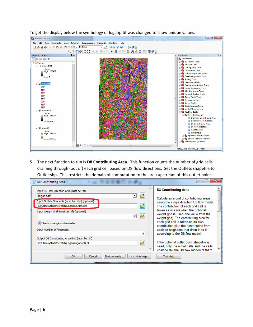
To get the display below the symbology of loganp.tif was changed to show unique values. 

  

5. The next function to run is D8 Contributing Area.  This function counts the number of grid cells 

draining through (out of) each grid cell based on D8 flow directions.  Set the Outlets shapefile to 

Outlet.shp.  This restricts the domain of computation to the area upstream of this outlet point.   

  

Page | 7 

The outlet point provided in the file Outlet.shp is at the location of the Logan River Stream Gauge based 

on latitude and longitude from the USGS NWIS information for that gauge 

(http://waterdata.usgs.gov/nwis/inventory/?site_no=10109000&agency_cd=USGS&)  

  

A multiplicative scale (100, 300, 1000, 3000 etc) is often best to render contributing area values as in the 

illustration below.   

 

  

Page | 8 

In the below I have added the Outlet.shp shapefile and zoomed to the area near the outlet to illustrate 

how watershed area has only been evaluated upstream of the outlet. 

  

Zoom in on the outlet and use the identify tool in ArcGIS 

  to identify the value of loganad8.tif at the location of the outlet.  Examine the properties of loganad8.tif 

and determine its cell size.   

 

To turn in:   

1. Report the contributing area draining to the outlet location in number of cells, square kilometers and 

square miles.  Report the area of a single grid cell.  Compare your result in square miles to the USGS 

drainage area value for this site. 

 

Save your map document, to save your work.  It is good practice to do this often in case of a crash. 

StreamNetworkAnalysisusingTauDEMfunctionsTauDEM provides a number of methods for delineating and analyzing stream networks and watersheds.  

The simplest stream network delineation method uses a threshold on contributing area.   

 

Page | 9 

6. Stream Definition by Threshold.  This function (in the stream network analysis tool group) defines a 

stream raster grid (src suffix) by applying a threshold to the input.  In this case the input is a D8 

contributing area grid and a threshold of 1000 grid cells has been used. 

  

The result depicts the stream network (but is not logically connected as a network shapefile yet). 

  

Page | 10 

7. Open Stream Reach and Watershed and select the following inputs.  Note that the stream reach 

shapefile name needs to be specified because the system for automatically generating output 

names does not work for shapefiles. 

  

Add the shapefile logannet.shp to ArcMap (other outputs are automatically added).   

 

You may get a warning "Unknown Spatial Reference".  Click OK.   

 

Page | 11 

This notifies you that the coordinate system of the stream network shapefile created by TauDEM is 

unknown.  This is a TauDEM shortcoming.  It does not assign coordinate systems to the shapefiles it 

outputs. 

 

Your display should be similar to the below, except without the highlighting of the area around Spawn 

Creek. 

  

The subwatershed raster and stream network shapefile are key outputs from TauDEM.  Each link in the 

stream network has a unique identifier that is linked to downstream and upstream links.  Each 

subwatershed also has a unique identifier that is referenced in terms of the stream network that it 

drains to.  This information enables construction of a subwatershed based distributed hydrologic model 

with flow from subwatersheds being connected to, accumulated in, and routed along the appropriate 

stream reaches.   

 

Zoom in on the area around Spawn Creek (see red box above) and examine the properties of the stream 

network and subwatersheds in this area.  There should be seven stream links that form the Spawn Creek 

tributary network. 

 

To turn in:   

2. Prepare a table that reports for the 7 stream links in the Spawn Creek tributary of the stream 

network the following attributes: 

- Link number 

Page | 12 

- Downstream link number 

- Upstream link number 1 

- Upstream link number 2 

- Downstream contributing area 

- Length 

- Identifier of corresponding watershed (WSNO) 

3. Open the attribute table of loganw and identify the count (number of grid cells) of the 7 Spawn Creek 

subwatersheds.  Based on this count calculate area of each subwatershed and reconcile your values 

with contributing area values in the table from the stream network.   

4. Prepare a diagram that shows, based on your answers to 4 and 5, how connectivity between 

subwatersheds, stream links and upstream and downstream links is encoded.   

 

3.LoganRiverHydrologicAnnualWaterBalanceandRunoffRatioexercise.Important quantities in the water balance of a watershed are the streamflow, expressed on a per unit 

area basis, area average precipitation and the runoff ratio r=q/P.  Let's determine these for the Logan 

River.  Streamflow we will get from the USGS.  Precipitation we will get from Oregon State University 

(PRISM). 

 

Use the USGS NWIS website for Logan River above state dam (10109000) 

http://waterdata.usgs.gov/nwis/nwisman/?site_no=10109000&agency_cd=USGS to determine mean 

annual streamflow for the years 1981‐2010.  These years chosen for consistency with PRISM.  Select 

annual statistics on this website and specify the period of record.  Then copy the data for each year to a 

spreadsheet and calculate the 30 year average.  Per unit area discharge is 

 

 

Do the necessary unit conversions to express this in mm. 

Page | 13 

PRISMPrecipitationdata.  From the Oregon State University PRISM website: 

http://prism.nacse.org/normals/ select precipitation and annual values and click on Download Data 

(.asc) 

 

You should receive a file PRISM_ppt_30yr_normal_800mM2_annual_asc.zip. 

Use a zip utility (I use 7zip) to uncompress this file.  The contents are: 

 

Page | 14 

In ArcGIS select the ASCII to Raster tool 

 

and use the following inputs 

 

This will result in a layer like the following being defined but it does not display properly geolocated with 

other data in ArcMap due to it not having a coordinate system specified (yet).   

Page | 15 

 

If you paid close attention you might have noticed that the PRISM zip file above included a file that 

ended in .prj.  This contains the needed coordinate system (projection) information. 

Open the Define Projection Tool in ArcMap 

 

Page | 16 

Select PrismPrecip Input Dataset or Feature Class.  Then click on the button next to Coordinate System 

 

At the window that opens select Import 

 

Find the Folder with the PRISM data and click on the PRJ file and click Add then OK twice to Define the 

projection from the PRJ file that was provided. 

Now if you zoom your map over Logan River you should be able to see the PrismPrecip Grid aligned with 

it.  I have symbolized it green to blue 

 

Page | 17 

Notice the higher precipitation values in the mountains.  These I symbolized with blue.  Notice also the 

data values in the legend table of contents.  These values are in mm (stated in one of the accompanying 

XML files).   

Next we would like to average this data over the Logan River Watershed.  To do this we need a single file 

specifying the "zone" that is the Logan River watershed.  The file loganw.tif defines subwatersheds.  

Make sure that under Customize Extensions, Spatial Analyst is checked. 

 

Use the Raster Calculator Tool 

 

Page | 18 

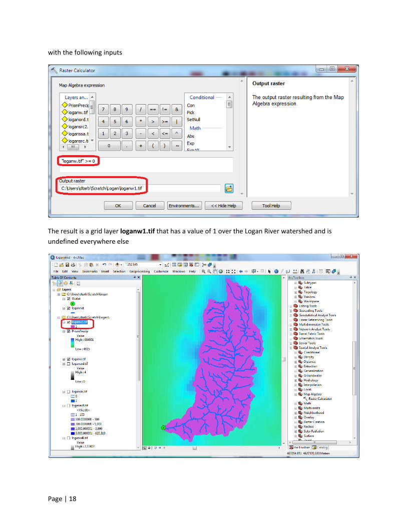
with the following inputs 

 

The result is a grid layer loganw1.tif that has a value of 1 over the Logan River watershed and is 

undefined everywhere else 

 

Page | 19 

Use the Zonal Statistics as Table tool 

 

with the following inputs 

 

Page | 20 

The result is a table giving precipitation statistics averaged over the Logan River Watershed. 

 

The mean rainfall over the Logan Watershed can be read as 941.1 mm.  (Beware.  Sometimes in ArcMap 

table displays you need to widen the column displays to get all digits displayed and interpret the data 

correctly). 

Calculate the runoff ratio for the Logan River 

 

To turn in:   

5. Report the following for the Logan River 

- mean annual discharge in cfs 

- mean annual runoff (discharge per unit area) in mm 

- Minimum, maximum and mean of mean annual precipitation over the Logan River 

watershed from PRISM in mm 

- Runoff ratio for the Logan River 

Page | 21 

4. SpawnCreekTOPMODELexerciseThis exercise sets up the data and guides you through the calculations involved in the Spawn Creek 

TOPMODEL runoff generation calculation that is Example 4 in the Rainfall Runoff Processes Module 

(http://hydrology.usu.edu/rrp/Document/index.asp?Parent=19#).  Spawn Creek is a tributary of the 

Logan River, so this exercise uses the same data as the Logan River Exercise above. 

1. Open a new ArcMap document and load loganp.tif and spawnoutlet.shp. 

  

2. Run D8 Contributing Area with the following inputs to isolate just the Spawn Creek watershed.   

 

Page | 22 

 

The result is illustrated below. 

  

In all the work above the single flow direction model D, was used, with flow being routed from each grid 

cell to only one neighbor.  TauDEM also uses the D (D‐Infinity) flow model that calculates the steepest 

outwards flow direction using triangular facets centered on each grid cell and apportions flow between 

neighboring grid cells based on flow direction angles.  This is useful for calculating specific catchment 

area used in TOPMODEL. 

 

3. The D‐Infinity Flow Directions function is starting point for all D‐Infinity work.  It calculates D‐Infinity 

flow directions for use in other TauDEM functions requiring D‐infinity flow direction input.  Run D‐

Infinity  Flow Directions with the following inputs.   

  

Page | 23 

D‐Infinity flow directions are encoded as angles counter clockwise from East in Radians as illustrated in 

the help 

  

Page | 24 

D‐Infinity flow directions render similar to a hillshading 

 4. The D‐Infinity Contributing Area function evaluates contributing area using the D‐Infinity model 

based on flow being shared between grid cells proportional to the angle to the steepest downslope 

direction.  This is designed to represent specific catchment area within dispersed flow over a smooth 

topographic surface. 

  

Page | 25 

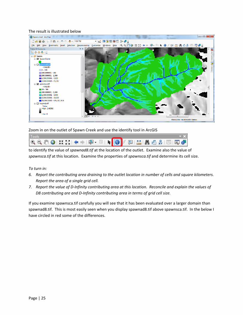
The result is illustrated below 

 

Zoom in on the outlet of Spawn Creek and use the identify tool in ArcGIS 

  to identify the value of spawnad8.tif at the location of the outlet.  Examine also the value of 

spawnsca.tif at this location.  Examine the properties of spawnsca.tif and determine its cell size.   

 

To turn in:   

6. Report the contributing area draining to the outlet location in number of cells and square kilometers.  

Report the area of a single grid cell.   

7. Report the value of D‐Infinity contributing area at this location.  Reconcile and explain the values of 

D8 contributing are and D‐Infinity contributing area in terms of grid cell size.   

If you examine spawnsca.tif carefully you will see that it has been evaluated over a larger domain than 

spawnad8.tif.  This is most easily seen when you display spawnad8.tif above spawnsca.tif.  In the below I 

have circled in red some of the differences. 

 

Page | 26 

  

This is because the D‐Infinity Contributing area function includes grid cells that only have part of their 

area draining to the outlet, while the D8‐Contributing Area Function includes only cells that drain 

entirely to the outlet using the D8 model. 

 

5. D8 Contributing area Mask.  To retain consistency in the area used in the calculations we will mask 

our calculations using the D8 contributing area.  The following Raster Calculator calculation results in 

a mask grid to use for these purposes 

  

Page | 27 

The result is illustrated below. 

  

The attribute table of spawnmask.tif indicates that this area contains 15782 grid cells, an area of 14.2 

km2.  These values are slightly different from the values in the module (Chapter 6:8) as the DEM may be 

slightly different, due to having been more recently downloaded from the National Elevation Dataset 

perhaps using a different projection.  These sort of small (0.2%) differences are not unusual in DEM 

analyses repeated for the same area with different data.  This exercise will follow Example 4 in the 

module but with the current DEM data. 

 

Assume the following hydrologic and parameter inputs 

Ko= 10 m/hr 

f= 5 m‐1 

e = 0.2 Qb = 0.8 m3/s 

 

Assume that we want to calculate the runoff due to 25 mm or rainfall. 

 

Page | 28 

6. Use the following raster calculation to evaluate wetness index, ln (a/S). 

  

The result is: 

  

Note that in the calculation I used the multiply by the mask to isolate the result to the masked area.  

Note also that I changed the color used to symbolize the mask to red and have this turned on behind the 

wetness index layer, spawnlnas.tif.  You can see red showing through in a few places.  These are 

locations where the slope is 0 and ln(a/S) results in no‐data.   

 

The following raster calculation determines how many grid cells are like this. 

Page | 29 

  

The result is 

  

The attribute table of the result indicates 15731 positive grid cells so there are 15782‐15731 = 51 grid 

cells with zero slope. 

 

The properties of spawnlnas.tif indicate the average value that is   in TOPMODEL theory. 

 

Page | 30 

7. Evaluate wetness index distribution.  spawnlnas.tif may be used to evaluate the distribution of 

wetness index through a series of raster calculations.  Select a manageable number of bin values 

(e.g. <4, 4‐6, 6‐8, 8‐10, ... 18‐20).  The number of grid cells in each can be evaluated using a raster 

calculation such as  

  

The result indicates only 5 grid cells in this case 

  

Use a series of these calculations to evaluate and plot a histogram of ln(a/S) for Spawn Creek  similar to 

the one in the Exercise on page 6:14 of the module. 

 

To turn in:   8. A histogram of wetness index distribution ln(a/S) for Spawn Creek. 

Page | 31 

 

8. Evaluate soil moisture deficit.  Evaluate D  using equation (85) from the module 

m)Tln(m)rln(mD o  

A raster calculation to evaluate soil moisture deficit D following equation (87) can then be set up:   

)S/aln(mDD  = 0.092 ‐ 0.04 x (ln(a/S) ‐ 6.904) 

 

Perform this calculation for your parameter values 

  

The result shows soil moisture deficit 

  

Page | 32 

The dark blue grid cells are saturated.  The light blue cells have soil moisture deficit less than 0.025 m so 

will saturate with 25 mm of infiltration.  The remaining grid cells would not saturate and would not 

generate runoff during our 25 mm storm. 

 

To turn in:   

9. Report the value of the TOPMODEL parameters   and D  for Spawn Creek and the conditions given.   

10. A neatly labeled layout map showing the soil moisture deficit for these conditions. 

A raster calculation can be used to determine the fraction of area that is saturated (D <= 0) which when 

combined with the flat area gives the area where there is no infiltration and all precipitation is runoff.   

 

Similarly a raster calculation can be used to isolate the area with D between 0 and 0.025 m.  This is the 

area that will saturate during the storm.  This raster calculation requires a bit of conditional logic and is 

  

Subtracting the average of smdwillsat.tif from 0.025 gives the average depth of runoff generated from 

this area, which when combined with the area gives the total runoff. 

 

To turn in:   11. The area and volume of runoff generated from flat areas for these conditions 

12. The area and volume of runoff generated from saturated areas for these condition   

13. The area and volume of runoff generated from areas that will saturate for these conditions 

14. The total volume and per unit area depth of runoff generated for these conditions 

15. The runoff ratio from this storm with these conditions  

Page | 33 

SummaryofItemstoturnin.1. Report the contributing area draining to the outlet location in number of cells, square kilometers and 

square miles.  Report the area of a single grid cell.  Compare your result in square miles to the USGS 

drainage area value for this site. 

2. Prepare a table that reports for the 7 stream links in the Spawn Creek tributary of the stream 

network the following attributes: 

- Link number 

- Downstream link number 

- Upstream link number 1 

- Upstream link number 2 

- Downstream contributing area 

- Length 

- Identifier of corresponding watershed (WSNO) 

3. Open the attribute table of loganw and identify the count (number of grid cells) of the 7 Spawn Creek 

subwatersheds.  Based on this count calculate area of each subwatershed and reconcile your values 

with contributing area values in the table from the stream network.   

4. Prepare a diagram that shows, based on your answers to 4 and 5, how connectivity between 

subwatersheds, stream links and upstream and downstream links is encoded.   

5. Report the following for the Logan River 

- mean annual discharge in cfs 

- mean annual runoff (discharge per unit area) in mm 

- Minimum, maximum and mean of mean annual precipitation over the Logan River 

watershed from PRISM in mm 

- Runoff ratio for the Logan River 

6. Report the contributing area draining to the outlet location in number of cells and square kilometers.  

Report the area of a single grid cell.   

7. Report the value of D‐Infinity contributing area at this location.  Reconcile and explain the values of 

D8 contributing are and D‐Infinity contributing area in terms of grid cell size.   

8. Report the value of the TOPMODEL parameters   and D  for Spawn Creek and the conditions given.   

9. A histogram of wetness index distribution ln(a/S) for Spawn Creek. 

10. A neatly labeled layout map showing the soil moisture deficit for these conditions. 

11. The area and volume of runoff generated from flat areas for these conditions 

12. The area and volume of runoff generated from saturated areas for these condition   

13. The area and volume of runoff generated from areas that will saturate for these conditions 

14. The total volume and per unit area depth of runoff generated for these conditions 

15. The runoff ratio from this storm with these conditions.